On the “Hysteresis Effects” observed by AMS02 in Cosmic Ray Solar Modulations

Abstract

The AMS02 collaboration has recently published high precision daily measurements of the spectra of cosmic ray protons, helium nuclei and electrons taken during a time interval of approximately 10 years from 2011 to 2020. Positron spectra averaged over distinct 27 days intervals have also been made public. The AMS02 collaboration has shown some intriguing ”hysteresis” effects observed comparing the fluxes of protons and helium nuclei or protons and electrons. In this work we address the question of the origin of these effects. We find that the spectral distortions generated by propagation in the heliosphere are significantly different for particles with electric charge of opposite sign (an effect already well established), with different behaviour before and after the solar magnetic field polarity reversal at solar maximum. This results in hysteresis effects for the $p/e^{-}$ comparison that follow the 22–year solar cycle. On the other hand particles with electric charge of the same sign suffer modulations that are approximately equal. The hysteresis effects observed for a helium/proton comparison can then be understood as the consequence of the fact that the two particles have interstellar spectra of different shape, and the approximately equal spectral distortions generated by propagation in the heliosphere have a rigidity dependence that is a function of time. These hysteresis effects can in fact be observed studying the time dependence of the shape of the spectra of a single particle type, and also generate short time loop–like structures in the hysteresis curves correlated with large solar activity events such as coronal mass ejections (CME’s). A description of solar modulations that includes these effects must go beyond the simple Force Field Approximation (FFA) model. A minimal, two–parameter generalization of the FFA model that gives a good description of the observations is presented.

I Introduction

The time dependence of the fluxes of Galactic cosmic rays generated by solar modulations Potgieter:2013pdj has been studied for several decades. During most of this time, the fundamental instrument to study these effects has been the neutron monitor simpson , but in recent years the PAMELA Adriani:2013as ; Martucci:2018pau ; Adriani:2015kxa ; Adriani:2016uhu and AMS02 ams_bartels_protons ; ams_bartels_electrons ; ams_daily_protons ; ams_daily_helium ; ams_daily_electrons ; ams_helium_isotopes detectors, located on satellites, have obtained precise direct measurements of the CR spectra that allow much more detailed analysis.

The AMS02 collaboration has published measurements of the spectra for four different particle types (protons, helium nuclei, electrons and positrons) averaged in time during 79 Bartels rotation of the Sun (each lasting 27 days) ams_bartels_protons ; ams_bartels_electrons , and more recently daily spectra for protons ams_daily_protons , helium nuclei ams_daily_helium and electrons ams_daily_electrons that extend for several years: 2824 spectra taken during a time period of 8.44 yr for $p$ and He, and 3193 spectra taken during a period of 10.45 yr for $e^{-}$, with both data sets starting on 2011-05–20. These data contain an enormous amount of information about the dynamics of the heliosphere and the properties of propagation of relativistic charged particles in it, and are the object of multiple studies.

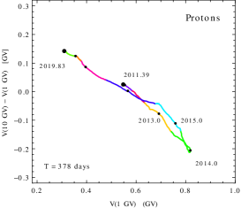
In their most recent papers the AMS02 collaboration has discussed some intriguing “hysteresis effects” observed comparing the time dependence of the fluxes for different particle types. In ams_daily_helium the ratio of helium and proton fluxes in some fixed rigidity ranges is studied as a function of the helium flux. Comparing moving averages of the two quantities with an integration time interval of 378 days (14 Bartels rotations) and one day step, the authors find that one value of the helium flux does not correspond to a unique value of the He/$p$ ratio (and therefore to a unique value of the proton flux). The time averaged He/$p$ ratio is found to be higher after solar maximum, and the authors conclude that at low rigidity the modulation of the helium to proton flux ratio is different before and after the solar maximum of 2014.

In ams_daily_electrons a similar study is performed for electron and proton spectra, comparing the time dependence of the two fluxes in the same rigidity intervals. Also in this case it is observed that one value of the $p$ flux does not correspond to a unique value of the $e^{-}$ flux. For long averaging time intervals (such as $T=378$ days or 14 Bartels rotations) one observes that, for the same proton flux, the electron flux is significantly smaller after solar maximum. The effect is similar to the one observed comparing the helium and proton spectra, but it is one order of magnitude larger. The study of moving averages of the fluxes with shorter integration times reveals additional structures in the time dependence for the $e^{-}/p$ ratio that appears to be associated to the presence of transients of solar activity, that are also the cause of rapid time variations of the fluxes of both particles. Studies of moving averages of the He/$p$ ratio with shorter time intervals have not been discussed in the AMS02 publications, but also this ratio exhibits time structures similar to those observed for the $e^{-}/p$ case.

In the following we want to address the problem of the origin of the “hysteresis” effects observed by AMS02. We will show that two essentially different mechanisms are operating. One mechanism is relevant for the long time scale dependence of the $e^{-}/p$ ratio, and has its origin in the well established fact that CR particles with electric charge of opposite sign travel along different trajectories that are confined in different regions of the heliosphere, and this results in different modulations effects. The heliospheric trajectories depend on the polarity of the solar magnetic field, and the reversal of the polarity at solar maximum is the origin of the large differences in the $e^{-}/p$ ratio before and after the solar maximum of 2014.

A second more subtle physical mechanism is at the origin of the hysteresis effects observed for the He/$p$ ratio, In this case the solar modulations for the two particle types are (in a sense that will be made more precisely below) in good approximation equal, and the hysteresis effects are the result of the fact that the spectral distortions generated by the modulations can have different rigidity dependences at different times.

This second mechanism can be observed, and is in fact more easily understood, studying the time dependence of the fluxes of one single particle type in two distinct rigidity intervals. The point is that observations of the same value of the flux at rigidity $\mathcal{R}_{1}$ can correspond (for different observations times) to different values of the flux at the rigidity $\mathcal{R}_{2}$. Therefore the plot of one flux versus the other [$J(\mathcal{R}_{2},t)$ versus $J(\mathcal{R}_{1},t)$] can exhibit non trivial “hysteresis” structures.

This mechanism generates similar effects also in the comparison of the fluxes $J_{p}(\mathcal{R},t)$ and $J_{\rm He}(\mathcal{R},t)$ of protons and helium at the same value of rigidity, even if the spectra of the two particles suffer the same modulations. This is because the effects of modulations must be understood not as an energy (or rigidity) dependent absorption effect, but instead as a distortion that acts on the local interstellar (LIS) spectra, and depends not only on state of the heliosphere, but also on the shape of the LIS spectra, that are different for protons and helium nuclei.

A simplified way to understand and model the solar modulations is to describe them as the effect of an average energy loss $\Delta E$ suffered by particles during propagation in the heliosphere. The hysteresis effects observed comparing the spectra of protons and electrons are due to the fact that the heliospheric energy losses for $p$ and $e^{-}$ are different and change in different ways during the solar cycle. On the contrary, the hysteresis effects observed comparing the spectra of protons and helium nuclei are due to the fact the their heliospheric energy losses (that have in good approximation the same time and rigitity dependences being related by the simple equation $\Delta E_{\rm He}=2\,\Delta E_{p}$) have a non trivial rigidity dependence that takes different shapes at different times.

This paper is organized as follows. In the next section we show how “hysteresis effects” are present in the AMS02 daily spectra measurements of all three particles (protons, helium nuclei and electrons) and can be observed studying the fluxes of each single particle type, with no need to compare different particle types. In the following section we introduce a very simple parametrization for the rigidity (or energy) spectra, that can describe surprisingly well the data for $p$, He, and $e^{\mp}$. This parametrization has two time independent parameters: a normalization and a spectral index that together define a simple power law in rigidity, and two time dependent parameters that determine a rigidity dependent potential that controls the modulation effects. Section IV presents the time dependence of the potentials for the different particles during the extended time interval of the PAMELA and AMS02 observations. Section V discuss the physical meaning of the modulation potential we have introduced, and the shape of the local interstellar (LIS) spectra of the CR particles. Section VI discusses the “loops” of different periods that emerge from different hysteresis studies. The final section summarizes the results.

II Flux correlations for a single particle type

The effect we want to investigate here is the shape of the distortions generated by solar modulations on the rigidity (or energy) spectrum of one particle type at different times. It is well known that at low rigidity the CR fluxes are time dependent, and for example the proton flux at $\mathcal{R}\simeq 1$ GV changes being highest (lowest) at the minimum (maximum) of solar activity. The question we want to address is if the value of the $p$ flux at 1 GV determines the entire spectrum at all rigidities or not. This is in fact the case in models that describe solar modulations in terms of only one time dependent parameter, such as the commonly used Force Field Approximation (FFA) Gleeson:1968zza , where a measurement of the flux at one rigidity (if it is in the range where the effects of the modulations are not negligible) is sufficient to determine the entire spectrum.

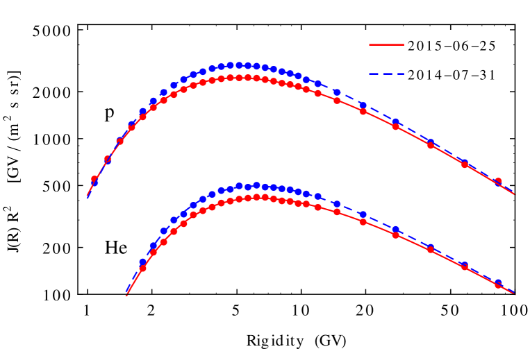
The AMS02 data however show that the assumption that solar modulation can be described by a single time dependent parameter is not correct. This conclusion emerges directly from the data, without any analysis. An illustration of this is presented in Fig. 1 that shows the proton spectra measured by AMS02 ams_daily_protons during two different days (2014–07–31 and 2016-06–25). The average fluxes measured during these two days are approximately equal for a rigidity of order 1 GeV, but differ by ($20\pm 1)$ % in the rigidity bin [4.88–5.37] GV. Fig. 1 also shows the spectra of helium nuclei measured by AMS02 ams_daily_helium during the same two days. One can note that the effects of solar modulations for protons and helium nuclei have the same qualitative features, as also the helium spectra are approximately equal ar $\mathcal{R}\simeq 1$ GV, and differ by $\sim 20$% at $\mathcal{R}\simeq 5$ GV. A more quantitative study, presented below, will show that the distortions to the proton and helium spectra (and in fact also to the positron spectrum) generated by solar modulations are in fact in very good approximation equal.

The observation that the flux at one rigidity $\mathcal{R}_{1}$ can correspond, at different times, to different fluxes at a second rigidity $\mathcal{R}_{2}$, suggests to explore the possibility to observe “hysteresis” effects such as those discussed by AMS02 (for the fluxes of two different particles measured in the same rigidity interval) ams_daily_helium ; ams_daily_electrons , also for the fluxes of one single particle type in two distinct rigidity intervals.

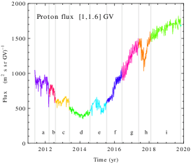
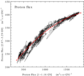
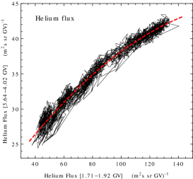
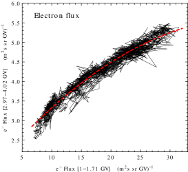
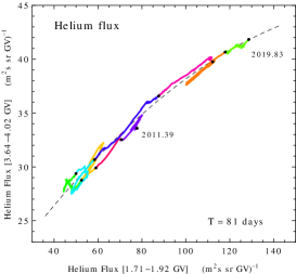
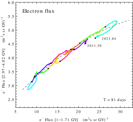
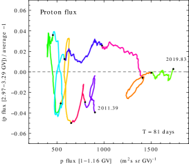
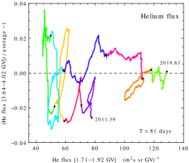
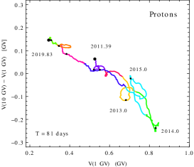
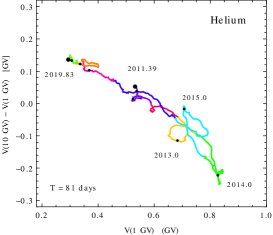
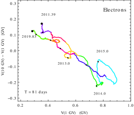
Some results of this type of study are illustrated in Fig. 2. The three panels in the top row of the figure show the time dependence of the flux of protons ams_daily_protons , helium nuclei ams_daily_helium and electrons ams_daily_electrons measured during different days in one fixed interval of rigidity ($\mathcal{R}=[1,1.16]$ GV for $p$, $[1.71,1.92]$ GV for He and $[1,1.71]$ GV for $e^{-}$). The measurements for protons and helium are taken for 2717 different days from 2011-05-20 to 2019–10–29, while the measurements for electrons are taken for 3193 days from the same initial day and extending to 2021–11-02.

The time interval of the daily spectra measurements covers a large part of the 24th solar cycle that extends from the minimum in December 2008 to the next minimum in December 2019 passing through a maximum around April 2014 (the $e^{-}$ measurements cover also the beginning of cycle 25th).

The fluxes for all three particle exhibit significant time variations on a variety of time scales, with the most prominent effect associated to the 11 year solar cycle. An important point is to note that, superimposed on the general trend of decreasing fluxes before solar maximum and increasing fluxes after maximum, other significant time variation structures associated to phases of enhanced or suppressed solar activity are present. For example, during the first part of the cycle (increasing solar activity and decreasing CR fluxes) one can identify three main local maxima of the flux, and during the second part of the cycle (decreasing solar activity and increasing CR fluxes) a prominent minimum of the fluxes is present in September 2017. In the three plots the colors and the vertical lines identify some time intervals associated with prominent time structures. These time intervals are labeled with a letter, with intervals (a), (b) and (c) roughly centered on the three local maxima in the first part of the cycle; intervals (d) and (e) covering the solar maximum part of the cycle; while the time interval around the prominent local minimum of September 2017 is labeled (h). The same colors are used in subsequent plots to identify the same time intervals.

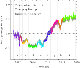
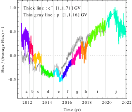
It is interesting to note that while the time dependences of the flux for the three particles ($p$, He and $e^{-}$) are qualitatively similar, the similarity is remarkably accurate for protons and helium nuclei, while there is an evident large difference between electrons and the two positively charged particles. To illustrate this point, the time dependences for helium nuclei and electrons are shown in the form $\phi(t)/\langle\phi\rangle-1$ (where the average is taken during the same time interval for all particles), and compared with the time evolution for protons.

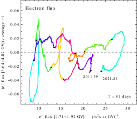
The nine panels in the lower part of Fig. 2 show the time evolution of the fluxes of protons, helium nuclei and electrons measured simultaneously in two distinct rigidity intervals. This is achieved studying the “trajectory” in time of the pair $\{J_{1}(t),J_{2}(t)\}$, where $J_{1}(t)$ and $J_{2}(t)$ are the fluxes measured at time $t$ in the two different rigidity intervals [$\mathcal{R}_{1},\mathcal{R}_{2}]$ and [$\mathcal{R}_{1}^{\prime},\mathcal{R}_{2}^{\prime}]$.

The three columns in Fig. 2 shows the trajectories of pairs of fluxes for protons (left), helium nuclei (middle) and electrons (right). In all three cases the lower rigidity interval is the same used to show the time evolution of the fluxes in the top row ($\mathcal{R}=[1,1.16]$ GV for $p$, $[1.71,1.92]$ GV for He and $[1,1.71]$ GV for $e^{-}$), while the second rigidity intervals are: $\mathcal{R}=[2.97,3.29]$ GV for $p$, $[3.64,4.02]$ GV for He and $[2.97,4.02]$ GV for $e^{-}$.

In the second row of panels, the time evolution of the pair of fluxes $\{J_{1}(t),J_{2}(t)\}$ is shown as a broken line that connects the daily measurements. There is of course a strong correlation between $J_{1}(t)$ and $J_{2}(t)$. This is expected because both fluxes are large (small) in periods of weak (strong) solar activity, however the trajectory is not limited to a narrow band, as expected if one assumes that the value of the flux $J_{2}(t)$ is determined by the value of $J_{1}(t)$. The spread of values of $J_{2}(t)$ for a fixed value of $J_{1}(t)$ is larger than the errors on the measurement (that are of order 1%, 1.5% and 2% for $p$, He and $e^{-}$ and are not shown to avoid cluttering), and therefore is physically significant.

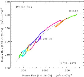
The trajectories that describe the daily flux measurements have a rich and complex structure that encodes very valuable information about CR propagation in the heliosphere, but because of their complexity are also difficult to interpret, and for this reason it is interesting to perform moving averages of the measurements, even if this procedure erases significant information about the time evolution of the spectra.

The third row of panels in Fig. 2 shows moving averages of the trajectories $\{J_{1}(t),J_{2}(t)\}$ for an averaging time interval of 81 days (3 Bartels rotations) and one day step. The panels in the bottom row show the same moving averages of the flux pairs but in a slightly different form, replacing the value of $J_{2}(t)$ with its deviation from an average value (shown as a dashed line in the two panels above). The resulting trajectories are much simpler, and reveal interesting structures in the time evolution of the spectra that are analogous (and in fact encode the same effects) of what has been observed by the AMS02 collaboration in the study of the He/$p$ and $e^{-}/p$ ratios.

The qualitative feature that is most evident in the figure is the presence of “hysteresis loops” in the trajectories that trace the evolution of the flux pairs $\{J_{1}(t),J_{2}(t)\}$. Inspecting Fig. 2 one can identify three such loops during the first part of the solar cycle (when solar activity is going toward maximum) that corresponds to the time intervals (a), (b) and (c) (following the notation indicated in the top row of the figure), and one loop during the second part of the solar cycle (when solar activity is decreasing after solar maximum), and corresponds to the time interval (h).

The “loops” are related to strong perturbations of the interplanetary magnetic field, superimposed to the more gradual 11 year solar cycle. The loops in the first part of the cycle are formed when the general decreasing trend of the two fluxes $J_{1}(t)$ and $J_{2}(t)$ is inverted and both fluxes increase during a short time interval before returning to their normal behavior of gradual decrease. The effect is faster and relatively larger for the flux in the high rigidity bin, generating a clockwise loop in the trajectory.

In the second part of the cycle (after solar maximum) a prominent loop is present around September 2017, when some large coronal mass ejections (CME) generate a large suppression of the CR fluxes during a time interval of several months. Also in this case the response of the flux in the high rigidity bin is larger and faster, resulting again in a clockwise loop in the trajectory of the flux pair.

It is straightforward to see how these loop structures in the time evolution of the CR spectra are also visible comparing the fluxes of two different particle types, as done in the AMS02 papers ams_daily_helium ; ams_daily_electrons .

The study of the rigidity dependence of solar modulations has been studied for decades, in particular in association with the so called Forbush decreases, sudden drops of the CR spectra (associated to CME’s or high-speed streams from coronal holes) first observed in 1937 forbush-1937 . Most of these studies have been performed with ground–based neutron monitor (NM) detectors. These instruments are located in regions with different geomagnetic cutoffs, and therefore can observe CR flux variations integrating over different rigidity ranges. Comparisons of the counting rates of different NM detectors have allowed to observe already in the 1970’s the presence of “hysteresis loops” associated to the rigidity dependent modulations hyst1 ; rajan_loops .

In more recent times spaceborne detectors placed in near Earth orbit have been able to measure directly the CR spectra of different particles (protons, helium nuclei and electrons by PAMELA Munini:2018cgc ; Lagoida:2021udw and electrons and positrons by DAMPE DAMPE:2021qet ) during major Forbush decreases, obtaining evidence that the CR fluxes recovery times are rigidity dependent and shorter at higher $\mathcal{R}$. The AMS02 data, thanks to its large statistics, high precision and a an extended data taking is of great value to develop a more complete understanding of the effects of perturbations in the interplanetary environment on the CR spectra.

III A two–parameter phenomenological description of solar modulations

The discussion in the previous section, as in the papers that present the AMS02 measurements, has been developed studying the time dependence of directly measured fluxes. This approach has the merit of avoiding the introduction of model dependent quantities and concepts, however it has also significant limitations. This is in part because it is not “economic”, since there are infinite ways to choose the rigidity or energy intervals used to study the evolution of the spectra, moreover, such a discussion cannot completely capture the properties of the modulation mechanism that generates distortions to the shape of the CR spectra.

In the following we will attempt to develop a simple parametrization of the CR spectra with the goal of extracting from the data few quantities that can capture the main effects of solar modulations. A convenient starting point is the widely used and very successful model of the Force Field Approximation (FFA) introduced by Gleeson and Axford Gleeson:1968zza . The fundamental assumption in the model is that CR particles traversing the heliosphere suffer a time dependent energy loss $\Delta E=|q|\,V(t)$ proportional to the absolute value of their electric charge. In the original version of the FFA, the same potential $V$ is valid for all particle types, but it is now well established that particles with electric charge of opposite sign propagate in different regions of the heliosphere and therefore “see” different potentials. The question if the same potential can describe the modulations of all particles that have electric charge of the same sign, should of course be tested experimentally.

If the LIS spectra at the boundary of the heliosphere are, as expected, isotropic and constant in time, it is then straightforward to derive an expression for the energy spectrum observable at the Earth at time $t$:

$$\phi(E,t)=\frac{p^{2}}{p_{0}^{2}}\;\phi_{0}[E+|q|\,V(t)]$$ (1)

In this expression $\phi_{0}(E)$ is the LIS spectrum, and $p$ and $p_{0}$ are the 3–momenta that correspond to the energies $E$ and $E+|q|\,V(t)$, that are the energies of a CR particle when detected at the Earth and entering the heliosphere.

In the FFA model the solar modulations are calculated in terms of the LIS spectrum $\phi_{0}(E)$, but the validity of the model can be tested without any knowledge of this spectrum, simply comparing spectra that are directly measurable at the Earth. In fact Eq. (1) implies that the spectra $\phi_{1}(E)=\phi[E,V(t_{1})]$ and $\phi_{2}(E)=\phi[E,V(t_{2})]$ observed at times $t_{1}$ and $t_{2}$ are related to each other by:

$$\phi_{1}(E)=\frac{p_{1}^{2}}{p_{2}^{2}}~{}\phi_{2}[E+|q|\,\Delta V(t_{1},t_{2})]$$ (2)

where $\Delta V(t_{,}t_{2})=V(t_{1})-V(t_{2})$ is the difference between the modulation potentials at times $t_{1}$ and $t_{2}$, and $p_{1}$ and $p_{2}$ are the momenta that correspond to the energies $E$ and $E+\Delta V$. The important point of Eq. (2) is that the two functions that enter the equality are directly measurable, and this allows to test the validity of the model without a knowledge of the LIS spectrum.

It is instructive to consider the ideal case of a LIS spectrum that is a simple power law in rigidity: $J_{0}(\mathcal{R})=K\,\mathcal{R}^{-\alpha}$. The modulated spectrum of a massless particle takes then the form:

$$J(\mathcal{R},V)=K\,\mathcal{R}^{2}\;(\mathcal{R}+|Z|\,V)^{-(2+\alpha)}$$ (3)

(with $Z=q/e$). This flux grows quadratically in $\mathcal{R}$ for low rigidities, reaches a maximum at $\mathcal{R}^{*}=2\,|Z|\,V/\alpha$, and for large rigidities becomes asymptotically a simple power law with constant spectral index $\alpha$. For a particle with mass $m$ the modulated flux takes the form:

$$J(\mathcal{R},V)=K\;|q|^{\alpha+3}\;\frac{\mathcal{R}^{3}}{E+m}\;(E+m+|q|\,V)\,(E+|q|\,V)^{-(\alpha+3)/2}\,(E+2m+|q|\,V)^{-(\alpha+3)/2}$$ (4)

(where $E=\sqrt{(q\mathcal{R})^{2}+m^{2}}-m$ is the kinetic energy that corresponds to rigidity $\mathcal{R}$). This form has shape similar to the massless case, with a flux that grows rapidly for small $\mathcal{R}$, reaches a maximum (at a rigidity that grows with $V$) and then, for large $\mathcal{R}$, becomes a power law of spectral index $\alpha$.

Expressing the spectrum in terms of kinetic energy, it takes the form:

$$\phi(E,V)=K\;|q|^{\alpha-1}\;E\;(E+2m)\,(E+m+|q|\,V)\,(E+|q|\,V)^{-(\alpha+3)/2}\,(E+2m+|q|\,V)^{-(\alpha+3)/2}~{}.$$ (5)

It should be stressed that the expressions (4) and (5) for a rigidity or kinetic energy spectrum might appear as rather complicated, but they describe a very simple model: an exact power law in rigidity (with normalization $K$ and spectral index $\alpha$) modulated by a constant energy loss $|q|\,V$. Adopting these expressions to fit the time dependent rigidity spectra measured by AMS02 and PAMELA is surprisingly successful.

Fitting the 2717 daily proton and helium daily spectra with data in the rigidity ranges [1–100] GV for $p$ (30 bins), and [1.71–100] GV for helium (26 bins) with the form (4) and allowing all three parameters ($K$, $\alpha$ and $V$) to be time dependent, one obtains reasonably good fits with global $\chi^{2}_{\rm min}/{\rm d.o.f.}=0.86$ for protons and 0.79 for helium nuclei. In the case of helium one has the problem that the flux is formed by a mixture of the two isotopes ⁴He and ³He ams_helium_isotopes . In this paper we have neglected the rigidity dependence of the isotopic composition, and assumed a constant ratio ³He/${}^{4}{\rm He}\simeq 0.2$.

For the electron daily spectra data, the AMS02 collaboration has released 3193 spectra in the rigidity range [1–42] GV. Selecting the smaller rigidity range $\mathcal{R}<10$ GV, the data can be successfully fitted with the expression (4) obtaining a global $\chi^{2}_{\rm min}/{\rm d.o.f.}=0.68$. In this case the range of the fit must be reduced because the $e^{-}$ spectrum has a hardening that begins at $\mathcal{R}\simeq 10$ GV ams_electrons .

Fitting the CR spectra with the form (4) and three time dependent parameters can be useful, but it is not entirely satisfactory, because it is not obvious how to interpret the time dependence of the three parameters $K$, $\alpha$ and $V$. If one tries to test a “minimal model” based on the FFA model, with $K$ and $\alpha$ constant and a time dependent (but constant in rigidity) potential one obtains fits that describe the data reasonably well, with deviations of order 10%, however, because of the remarkable accuracy of the AMS02 and PAMELA measurement (with errors of order 1–3%), the quality of the fits are poor.

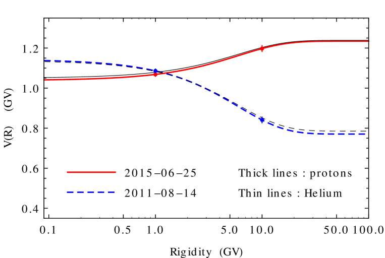
This suggests to introduce a simple generalization of the FFA model, that is always based on expression Eq. (4) to fit the rigidity spectra, but keeping $K$ and $\alpha$ as time independent (because they are considered as parameters associated to the LIS spectra) and introducing a rigidity dependence for the potential $V(t)$. For this purpose we introduce the form:

$$V(\mathcal{R},t)=V_{0}(t)+[V_{\infty}(t)-V_{0}(t)]~{}(1-e^{-\mathcal{R}/\mathcal{R}^{*}})$$ (6)

that contains two time dependent parameters $V_{0}(t)$ and $V_{\infty}(t)$ that can be interpreted as the average energy losses (divided by $|q|$) during propagation in the heliosphere for particles that arrive at the Earth with very small and very large rigidities. It is also possible to express the potential in terms of $V_{1}=V(\mathcal{R}_{1})$ and $V_{2}=V(\mathcal{R}_{2})$, that are the values of $V$ for two (arbitrary, but conveniently chosen) rigidities:

$$V(\mathcal{R},t)=\frac{e^{-\mathcal{R}/\mathcal{R}^{*}}}{e^{\mathcal{R}_{1}/\mathcal{R}^{*}}-e^{\mathcal{R}_{2}/\mathcal{R}^{*}}}~{}\left[V_{1}(t)\;\left(e^{(\mathcal{R}+\mathcal{R}_{1})/\mathcal{R}^{*}}-e^{(\mathcal{R}_{1}+\mathcal{R}_{2})/\mathcal{R}^{*}}\right)-V_{2}(t)\;\left(e^{(\mathcal{R}+\mathcal{R}_{2})/\mathcal{R}^{*}}-e^{(\mathcal{R}_{1}+\mathcal{R}_{2})/\mathcal{R}^{*}}\right)\right]$$ (7)

The AMS02 data are published for rigidities larger than 1 GV, and the effect of modulations are small and difficult to measure for $\mathcal{R}\gg 10$ GV, and therefore in the present paper, we have chosen to parametrize the energy dependence of the potential with $V_{1}=V(1~{}{\rm GV})$ and $V_{2}=V(10~{}{\rm GV})$. The potential in Eq. (7) also contains the additional parameter $\mathcal{R}^{*}$, that is kept constant with value $\mathcal{R}^{*}=6$ GV .

In the remaining of this paper we will fit the lower rigidity part of the CR spectra for protons, helium nuclei electrons and positrons with the scheme we have outlined, that is using Eq. (4) with a a time dependent potential of form (7). For the two parameters $K$ and $\alpha$ that describe the power law spectra, we have used the average values $\langle K\rangle$ and $\langle\alpha\rangle$ obtained from fits to all AMS02 spectra based on Eq. (4) with all three parameters $K$, $\alpha$ and $V$ free (and $V$ constant in rigidity). The results are: $K=2.94$, 0.426, 0.743 and $5.01\times 10^{-3}$ [in units (cm²  s  sr  GV)^-1] and $\alpha=2.90$, 2.80, 4.10 and 3.42 for $p$, He, $e^{-}$ and $e^{+}$ respectively.

With this scheme one obtains reasonably good fits to all AMS02 and PAMELA observations. For example, the global chi squared of fits to the AMS02 daily spectra are $\chi^{2}_{\rm min}/{\rm d.o.f.}=0.82$, 0.76 and 0.71 for $p$, He and $e^{-}$. These values are approximately equal to those obtained using Eq. (4) with three time dependent parameters: $K$, $\alpha$ and (constant in rigidity) $V$, but the interpretation of the parameters is now more natural.

Four examples of fits to the AMS02 measurements (two for $p$ spectra, and two for He spectra) are shown in Fig. 1, where one can see that they give a good description of the data. The rigidity dependent potentials with form (7) that enter the expression for the rigidity spectrum of Eq. (4) are shown in Fig. 3, where the points show the best fit values of the parameters $V_{1}$ and $V_{2}$. One can see that the potentials have a modest but significant rigidity dependence with a form that is different for spectra observed at different times. It is remarkable that the potentials obtained fitting the $p$ and He spectra measured the same day are (within errors) equal to each other. This is in fact a result that is in general valid for all the $p$ and He daily spectra measured by AMS02, indicating that the solar modulations for protons and helium nuclei are in good approximation equal. It should be noted that the potential that enters the expression of Eq. (4) for the modulations is multiplied by the absolute value of the electric charge of the particles, therefore this result can also be stated saying that (in an appropriate sense) the effects of solar modulations are two times larger for helium (that has charge number $Z=2$) .

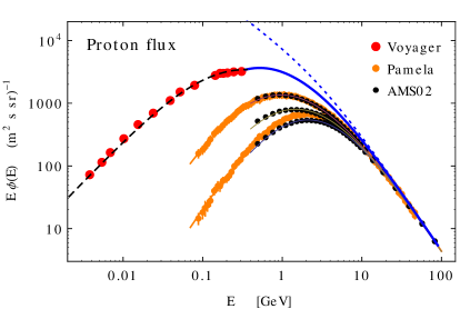
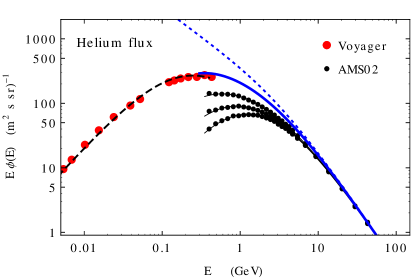
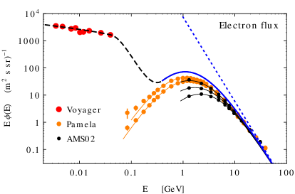
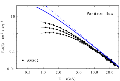
Some other examples of fits to AMS02 and PAMELA spectra for protons, helium nuclei, electrons and positrons calculated in the scheme we are discussing here are shown in Fig. 4. In the figure the spectra and their fits are shown, as function of kinetic energy, in four separated panels, where the power law rigidity spectra that enters the expression of Eq. (5) are also shown as dashed lines. In three panels (for $p$, He and $e^{-}$) we also show the measurements obtained by Voyager 1 after crossing the heliopause at a distance of approximately 120 AU from the Sun voyager-2016 that are considered as representative of the CR spectra in the local interstellar medium.

Each one of the panels include three spectra from AMS02. For $p$, He and $e^{-}$ the three spectra are the highest, the lowest and an intermediate one, chosen among the daily measurements ams_daily_protons ; ams_daily_helium ; ams_daily_electrons . For positrons, the three spectra are again the highest, lowest and an intermediate one, but chosen among the measurements obtained averaging over one Bartels rotation ams_bartels_electrons . In the panels for $p$ and $e^{-}$ we include two spectra (the highest and lowest) obtained by PAMELA Adriani:2013as ; Martucci:2018pau ; Adriani:2015kxa with longer averaging times. The PAMELA results are of great interest because they cover a different time interval (June–2006 to January–2018) and because they are available in a kinematic range that extends to lower rigidities. Our model gives a good description also of the lower rigidity observations of PAMELA, with significant deviations only for the electron spectra at $E\lesssim 200$ MeV.

IV Time dependence of the Potentials

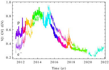
The time dependence of the potentials obtained fitting the daily spectra measured by AMS02 for protons, helium nuclei and electrons are shown in Fig. 5. The potentials in the figure include the subtraction of a constant shift that depends on the particle type: ($\Delta V_{\rm LIS}=0.29$, 0.30 and 1.14 GV for $p$, He and $e^{-}$ respectively) that will be discussed in the next section.

The top–left panel in Fig. 5 shows the potential $V_{1}=V_{[1~{}{\rm GV}]}$ for protons and electrons. The two potentials have significantly different time dependences, and with the shifts that we have introduced are approximately equal during the time interval, in the middle of 2014, that corresponds to the reversal of the polarity of the solar magnetic field. One also has (for both rigidities 1 GV and 10 GV) the inequalities:

$$\begin{cases}V^{(e^{-})}(t)<V^{(p)}(t)&\text{for}~{}~{}t<t_{\rm reversal}\\[3.41418pt] V^{(e^{-})}(t)>V^{(p)}(t)&\text{for}~{}~{}t>t_{\rm reversal}\end{cases}$$ (8)

At the reversal time $t_{\rm reversal}$ the solar magnetic field polarity changes from negative ($A=-1$) to positive ($A=+1$). During a phase of negative polarity particles with electric charge $q<0$ arrive at the Earth from the heliospheric poles, while particles with $q>0$ arrive travelling close to the heliospheric equator and the wavy current sheet. The situation is reversed after the flip of the magnetic field polarity. Our results are therefore consistent with the expectation that the energy losses during propagation in the heliosphere are larger for particles that arrive from the heliospheric equator Potgieter:2013pdj ; Lipari:2014gfa .

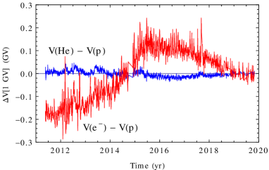
The top–right panel in Fig. 5 shows the differences between the potentials at rigidity 1 GV of electrons and protons and of helium nuclei and protons. It is striking that the potentials of $p$ and He are approximately equal. This result has important implications, because it validates the idea of using a potential to describe solar modulations, and is consistent with models where protons and helium nuclei of equal rigidities follow (approximately) equal trajectories in the heliosphere.

The bottom–left panel in Fig. 5 shows the time dependence of the potential differences $\Delta V=V_{[10~{}{\rm GV}]}-V_{[1~{}{\rm GV}]}$ for protons and electrons. The rigidity dependence of the potentials is rather small (with $|\Delta V|\lesssim 0.25$ GV), so that a simple FFA parametrization can be considered, for many applications, a reasonable approximation, validating many studies performed in the past, however the introduction of a rigidity dependence is necessary to obtain good quality fits. It is also important to note that $\Delta V$ can be either positive or negative at different times, so that the modulated spectra can have different shapes at different times.

The bottom–right panel in Fig. 5 shows the difference between $\Delta V$ for electrons and protons, and for helium nuclei and protons. One can note that the rigidity dependences of the potentials for electrons and protons are strongly correlated but not identical. This can be understood as the consequence of the facts that in general the properties of the (different) regions of the heliosphere where particles of opposite electric charge propagate are correlated, for example because the same CME’s can perturb both regions. The difference in $\Delta V$ between protons and helium nuclei is much smaller, and again indicates that the solar modulation effects are in good approximation equal for the two particles.

To study positron solar modulation we have fitted the AMS02 measurements of $p$, He, $e^{-}$ and $e^{+}$ spectra obtained averaging over 27 days ams_bartels_protons ; ams_bartels_electrons . The results are shown in Fig. 6. In the top–left panel the proton potential at rigidity $\mathcal{R}\simeq 1$ GV is compared to the one obtained fitting the daily spectra to show the consistency of the results. In the top–right panel the potentials (always at 1 GV) for the four particles ($p$, He, $e^{-}$ and $e^{+}$) are shown together, with the potential for positrons shifted by $\Delta V_{\rm LIS}^{(e^{+})}\simeq 0.176$ GV). The potentials for the three positively charged particles ($p$, He and $e^{+}$) are in good approximation equal, while the potential for $e^{-}$ is significantly different.

It should be noted that one expects that the modulations of particles with the same electric charge but different mass cannot be identical, with differences that increase in importance for low rigidities. The differences in modulation are expected because the relation between energy and rigidity is mass dependent, so that particles of different mass that enter the heliosphere at the same point with the same initial $\mathcal{R}_{i}$ will develop different rigidities due to energy losses, and travel along different trajectories. In addition, particles with identical rigidity but different mass will have different velocities and therefore different propagation times in the heliosphere, and this can also result in different modulations if the heliosphere is not in a stationary state. Our analysis shows only small differences in the potentials for protons and helium (at the level of a few percents). Future studies of these mass dependent effects that include helium nuclei will also have to take into account their rigidity dependent isotopic composition.

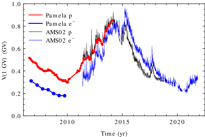
The results of the potentials at 1 GV for fits to the PAMELA protons (83 spectra Adriani:2013as ; Martucci:2018pau ) and electrons (7 spectra Adriani:2015kxa ) are shown, together with the fits to the AMS02 daily spectra, in Fig. 7. The PAMELA data start in June 2006, and cover also the final part of solar cycle 23. The measurements of the proton spectra extend to the beginning of 2014, and can be compared with the first part of the AMS02 data. The agreement between the two data sets is good. The measurements of the $e^{-}$ spectrum extend only to 2009, and such a comparison is not possible.

V The Local Interstellar Spectra

It is now desirable, indeed necessary, to address the question of what physical meaning can be attributed to the potentials we have obtained fitting the AMS02 and PAMELA data, and what can be deduced from these studies about the CR interstellar spectra.

In the FFA model the physical meaning of the (rigidity independent in the original formulation) potential is clear: it gives the average energy loss (divided by $|q|$) suffered by CR particles in their propagation from the boundary of the heliosphere to the Earth. In the model discussed here the potential describes a spectral distortion calculated with respect to an “artificial” spectrum, that has a simple power law form in rigidity, and therefore this potentials does not have a well defined physical meaning. However, the difference $\Delta V(\mathcal{R},t_{1},t_{2})=V(\mathcal{R},t_{1})-V(\mathcal{R},t_{2})$ between potentials obtained from fits to the spectra measured at times $t_{1}$ and $t_{2}$, is related to the two observed spectra via Eq. (2), and can be interpreted as the difference in the average energy loss suffered during heliospheric propagation by particles observed with rigidity $\mathcal{R}$ at times $t_{1}$ and $t_{2}$. The simple power law spectrum “cancels” in this comparison, as it plays the role of a “scaffolding”, used to perform the fits and obtain the potentials, and that can then be discarded.

This procedure leaves the LIS spectra undetermined, and this is a serious limitation because the determination of the interstellar spectra is a fundamental goal in the study of solar modulations.

There is a large literature about estimating the shape of the cosmic ray LIS spectra (see for example Boschini:2017fxq ; Bisschoff:2019lne ) and in all these studies the measurements obtained by Voyager 1 beyond the heliopause voyager-2016 play a crucial role. One should however note that the Voyager data, while of great value, are not sufficient to allow a model independent determination of the LIS spectra. This is because the Voyager data cover only a limited kinematical range (a maximum observed energy of 350 MeV for protons, and 75 MeV for electrons). Since the energy lost by CR particles traversing the heliosphere is of order 300 MeV or more, it follows that the CR particles in the range observed by Voyager do not reach the Earth, and vice–versa the particles in the energy range of observations at the Earth arrived at the boundary of the heliosphere with energy above the range of the Voyager measurements, and therefore a direct comparison of shapes of the spectra formed by the same particles in interstellar space and at the Earth is not possible.

The Voyager data are of course a very important constraint in the construction of the LIS spectra. The importance of this constraint is evident comparing the spectra in Fig. 4. For example inspecting the top–left panel in the figure one can see that the proton rigidity power law spectrum (shown as a dotted line) used as a starting point in the fitting procedure, is clearly much larger that the LIS spectrum. On the other hand, distorting this power law spectrum with a rigidity independent potential of 0.29 GV one obtains (thick solid line) a spectrum that joins smoothly the Voyager data.

The same considerations are valid for the helium spectrum, where distorting the power law spectrum with a rigidity independent potential of 0.30 GV one obtains a flux that joins smoothly the Voyager data (see the top–right panel in Fig. 4).

This suggests that the LIS spectra for protons and helium can be, in first approximation, described by a power law in rigidity distorted by a rigidity independent potential $\Delta V_{\rm Lis}$. The potential $V_{\rm fit}(\mathcal{R},t)$ obtained from a fit connects the spectrum observed at time $t$ to a simple power law spectrum; subtracting the shift $\Delta V_{\rm LIS}$ one obtains a potential $V(\mathcal{R},t)$ that connects the observed and the interstellar spectra, and therefore (in first approximation) describes the energy losses of the CR particles during heliospheric propagation:

$$V(\mathcal{R},t)\simeq V_{\rm fit}(\mathcal{R},t)-\Delta V_{\rm LIS}~{}.$$ (9)

Extending these considerations to the electron spectra poses some very interesting problems. A first consideration is that, as already discussed, we expect that the potentials for particles with electric charge of opposite sign will in general be different. This is because the trajectories of charged particles are also determined by the regular heliospheric magnetic field, and particles with opposite electric charge will propagate in different regions of the heliosphere, where they can suffer different energy losses. At solar maximum however, during the reversal of the heliospheric magnetic field polarity, the regular field is negligible, and the trajectories of the CR particles are controlled only by the random field. This implies that during the duration of the polarity reversal, the potentials for particles of opposite electric charge should be approximately equal. Imposing the constraint:

$$\langle V^{(e^{-})}\rangle_{\rm reversal}=\langle V^{(p)}\rangle)_{\rm reversal}$$ (10)

for averages of the potentials during the field polarity reversal (that is approximately the time interval from May to July 2014), we arrive to an estimate of the potential shift required for electrons: $\Delta V_{\rm LIS}^{(e^{-})}\simeq 1.14$ GV.

The electron LIS spectrum calculated with this shift is shown in the bottom–left panel of Fig. 4. To connect this estimate of the LIS spectrum to the Voyager data (that are available only at very low energy: $E\lesssim 75$ MeV) seems to require a non trivial spectral shape, perhaps indicating the presence of an additional low energy component in the electron spectrum.

For positrons no measurements at large distance from the Sun are available to constrain the shape of the $e^{+}$ LIS spectrum, however it is possible to estimate the shift $\Delta V_{\rm LIS}^{(e^{+})}$ comparing fits to the $p$ and $e^{+}$ spectra taken simultaneously and averaged over one Bartels rotation ams_bartels_protons ; ams_bartels_electrons . The potentials for $p$ and $e^{+}$ are shown in Fig. 6, and are consistent with a constant difference:

$$V_{\rm fit}^{(e^{+})}(\mathcal{R},t)\simeq V_{\rm fit}^{(p)}(\mathcal{R},t)-0.124~{}{\rm GV}~{}.$$ (11)

suggesting that the $\Delta V_{\rm LIS}^{(e^{+})}\simeq\Delta V_{\rm LIS}^{(p)}-0.124$ GV. Adopting this shift one obtains for positrons the LIS spectrum shown with the thick solid line in the bottom–right panel in Fig. 4.

The estimates of the LIS spectra obtained in this section are only tentative, and are not justified by a theoretical model, and therefore of limited value. In particular, the assumption that $\Delta V_{\rm LIS}$ is rigidity independent does not have a good justification, except for the fact that it results, for all the four particle types considered here ($p$, helium nuclei, $e^{\mp}$), in a remarkably simple form for the LIS spectra, with a shape determined by only two parameters (the spectral index $\alpha$ and the potential $\Delta V_{\rm LIS}$). The possible implications of this result deserve a more detailed study.

The study of the shape of the $e^{\mp}$ LIS spectra is of particular importance because different models predict that in the kinematical range where solar modulations are important ($0.1\lesssim\mathcal{R}\lesssim 10$ GV) one should observe spectral structures, associated for example to the critical energy where energy losses during interstellar propagation become the dominant sink mechanism for $e^{\mp}$ (overtaking escape from the Galaxy) Lipari:2018usj , or the critical energy where a new source mechanism (such as acceleration in Pulsars) becomes the dominant one DiMauro:2023oqx . The simple shape of the $e^{\mp}$ LIS spectra suggested by our study disfavours these possibilities.

VI Hysteresis loops

VI.1 The 22–year solar cycle

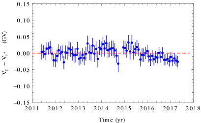
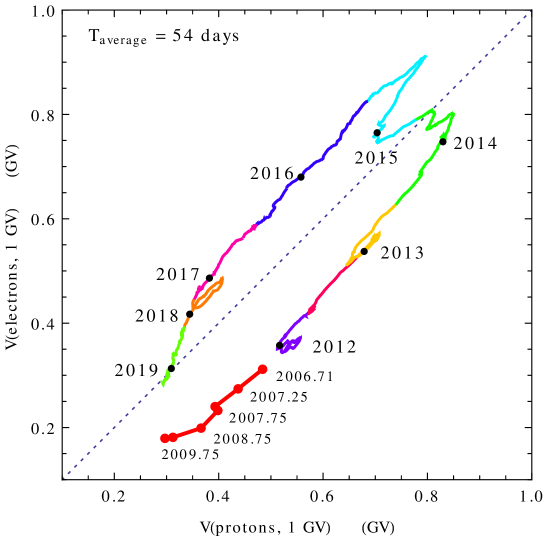
An instructive way to compare the proton and electron potentials is shown in Fig. 8, where the top panel shows the trajectory of the point $\{V_{p}(t),V_{e^{-}}(t)\}$ that represents the potentials at rigidity 1 GV obtained fitting electron and proton spectra measured at the same time $t$ by PAMELA or AMS02. For the PAMELA data the plot shows the potentials obtained fitting the seven electron spectra in Adriani:2015kxa ; Adriani:2016uhu , together with an interpolation of the potentials obtained fitting the proton spectra Adriani:2013as ; Martucci:2018pau . The PAMELA measurements are in the time interval from July 2006 to October 2009 and cover the last part of solar cycle 23 when solar activity goes toward its minimum, with polarity $A<0$. For the AMS02 data we show the results of fits to all days where both $p$ and $e^{-}$ spectra have been measured, with the broken line connecting all measurements (in order of increasing time). The AMS02 data start in May 2011, and covers most of solar cycle 24, including the phase of solar maximum where one observes the reversal of the solar magnetic field polarity.

Inspecting Fig. 8 one can observe some striking features, with the trajectory of the potential pair $\{V_{p}(t),V_{e^{-}}(t)\}$ that draws a loop. From the beginning of the AMS02 observations until the solar maximum around the middle of 2014 (a period where $A<0$), both potentials $V_{p}(t)$ and $V_{e^{-}}(t)$, averaging over fluctuations, grow gradually at approximately the same rate but with $V_{e^{-}}(t)<V_{p}(t)$. The time interval 2014–2016 corresponds to an extended solar maximum phase and shows an evident double peak structure separated by a gap, a structure that is also observed in other solar cycles. During this phase of the cycle the proton potential reaches its maximum before the potential for electrons. In the subsequent phase of the cycle (with positive polarity $A>0$) both potentials decrease, again at approximately the same rate, but the inequality for the potential is reversed ($V_{e^{-}}(t)>V_{p}(t)$).

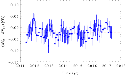
In the top panel of Fig. 8 the complicated form of the line that connects the potentials for the AMS02 daily spectra encodes valuable information, but performing moving averages of the two potentials allows to obtain the much simpler trajectory, shown in the bottom panel, where the “global loop” of the trajectory is more clearly visible.

The data strongly suggests that the point $\{V_{p}(t),V_{e^{-}}(t)\}$ travels along the loop in a clockwise sense for cycles (like solar cycle 23) where the magnetic field polarity at the start of the cycle (that is at solar minimum) is positive, and in an anti–clockwise sense for cycles (like solar cycle 24) where the situation is opposite.

In fact, in Fig. 8, one can observe that in the time interval where only the PAMELA data are available both potentials decrease gradually (with $V_{e^{-}}(t)<V_{p}(t)$), and the pair $\{V_{p}(t),V_{e^{-}}(t)\}$ completes (around the end of 2006) a clockwise loop at the solar minimum that separates solar cycles 23 and 24. After a gap in the observations of approximately 1.6 years, the AMS02 become available during the growing phase of solar cycle 24, and one observes a reversal of the trajectory with both potentials growing (with $V_{e^{-}}(t)<V_{p}(t)$ as before) and therefore moving in an anti–clockwise sense along the loop.

If this scenario is correct, during the current solar cycle (number 25) that started around December 2019, one should observe the point that represents the potential pair to move in clockwise sense along a loop that during the initial phase of increasing solar activity has $V_{e^{-}}>V_{p}$.

VI.2 Solar activity transients

In the bottom panel of Fig. 8 are also evident some loop–like structures of shorter time scale, that are in coincidence with similar structures observed for the flux–flux correlations of a single particle (as discussed in section II and illustrated in Fig. 2).

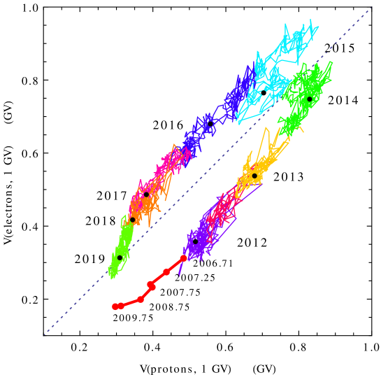
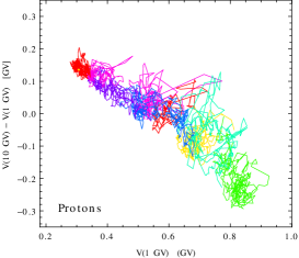
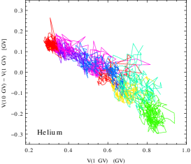
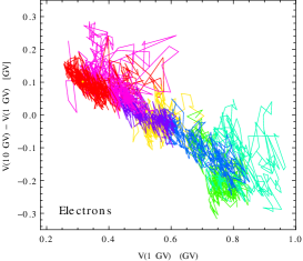
These effects can be also observed studying correlations between the values of the potential at different rigidities. This is illustrated in Fig. 9 that shows the trajectory of the point $\{V_{1}(t),\Delta V(t)\}$ where $V_{1}=V_{[1~{}{\rm GV}]}$ and $\Delta V=(V_{[10~{}{\rm GV}]}-V_{[1~{}{\rm GV}]})$ that describes the time evolution of the potentials obtained fitting the daily spectra measured by AMS02 for protons, helium nuclei and electrons. In the three panels at the top the broken line connects the results of the fits to the daily spectra for the three particle types (the errors are not shown to avoid clutter). One can note that for a fixed value of $V_{1}$, the value of $\Delta V$ is not unique but it has a finite range. The three panels in the middle row of the figure show moving averages of the potential after integration over time intervals of 81 days (three Bartels rotations). The simplification obtained performing the moving average allows to make evident some interesting “hysteresis structures”. These structures are of course the same ones visible in the flux–flux correlations of Fig. 2, it is however interesting to note that the modulation potential describes the state of the heliosphere, and is independent from the shape of the spectra of the particles in interstellar space.

Inspecting Fig. 9 one can see that the hysteresis effects for protons and helium are approximately equal, while the effects for electrons, while strongly correlated, are significantly different. This can be understood noting that the same solar activity events, such as large CME’s, can perturb both of the (different) regions of the heliosphere where protons and electrons are propagating, resulting in effects on the $p$ and $e^{-}$ spectra that are correlated but not identical.

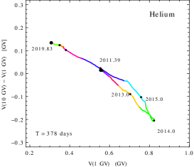
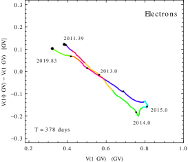
The three panels in the bottom row of Fig. 9 show the trajectories of the potentials for moving averages with a long integration time of 378 days (14 Bartels rotations). For all three particles ($p$, He and $e^{-}$) one can see some significant differences (with the same qualitative structure) for the average potentials during phases of the solar cycle before and after solar maximum. This effect is the same that was observed by AMS02 in ams_daily_helium studying the helium/proton ratio. It is difficult to say at the moment what is the origin of the effect, and if it is associated to the ensemble of the solar transient events in the solar cycle under study, or is related to the general properties of the 22–year solar cycle.

As already discussed, performing moving averages (of fluxes as in Fig. 2, or of potentials as in Fig. 9) allows the visualization of interesting structures in CR modulation, but also erases valuable information encoded in the evolution of modulations for time scales shorter than the averaging time.

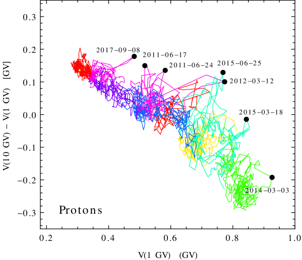
To illustrate this point in Fig. 10 we show again the detailed (day to day) trajectory of the potential parameters $\{V_{1}(t),\Delta V(t)\}$ for protons, indicating few (seven) days that correspond to major solar events. These events have also resulted in Forbush decreases observed by neutron monitors. To each events corresponds an large increase in the modulation potentiala, and remarkably the increase of the potential at the higher rigidity (10 GV) is stronger than at the lower one (1 GV). These effects (as discussed in section II) have been revealed in the past rajan_loops ; Munini:2018cgc ; Lagoida:2021udw ; DAMPE:2021qet , but a detailed explanation is still under construction.

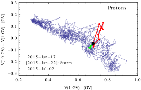
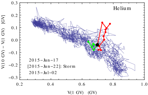
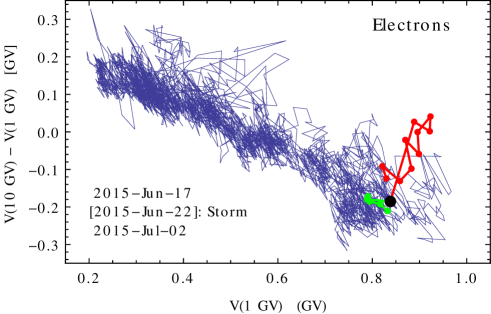
The effects of large solar activity events on the CR spectra can evolve very rapidly on a time scale of hours, and following the details of this evolution, can be of great help to develop an understanding of these phenomena. the AMS02 daily measurements are therefore of great interest. As an example, in Fig.11 we show the the trajectory of the modulation potentials (for $p$, He and $e^{-}$) obtained fitting the AMS02 daily spectra obtained during few days around one of the largest solar events during solar cycle 24. This event was observed around the summer solstice of 2015 event-summer-solstice-2015 . From 18–23 June, one of the largest sunspot active regions in the Sun (AR 12371), at the time directly facing Earth, produced several flares, giving origin of four CME impacting Earth in the period 21-25 June. The third and largest impact (June 22nd) generated a G4-severe geomagnetic storm with spectacular auroras even at low latitudes, followed by a Forbush decrease observed by ground-level detectors. Fig. 11 puts in evidence the trajectories of the modulation potential for $p$, He and $e^{-}$ (represented by the pair $\{V_{1}(t),\Delta V(t)\}$) taken during a time interval of 16 days around the date of the solar storm (starting 5 days before, and ending 10 days after). A detailed description of this event is not possible here, but one can note that it generated distortions of the spectra for all three CR particles of very similar structure. The spectral distortions generated by the event developed rapidly, with a time scale of one day or less; following this, the spectra returned to their pre-solar-event values with a longer time scale of several days. As noted before, the distortions (measured by the variation of the modulation potential) were larger at the higher rigidity of 10 GV, and weaker at $\mathcal{R}\simeq 1$ GV, and this appears to be the case in most if not all cases. Time structures qualitatively similar to what we have described can be observed for other large solar activity events.

VII Summary and Conclusions

Most of the already rich literature that discusses the PAMELA and AMS02 data is based on the study of the time dependence of the CR fluxes in different intervals of rigidity (or energy). An alternative possibility, it to extract from the data some time dependent parameters that describe the CR spectral shapes. In this work we have used this second approach, and demonstrated that it is possible to accurately and economically describe the CR spectra of each particle type in terms of a time dependent modulation potential $V(\mathcal{R},t)$. A small (but not negligible) rigidity dependence of the potential is required to fit the high precision data that are now available.

The main goal of this work has been to investigate the origin of the phenomena observed by the AMS02 collaboration and called “hysteresis effects”. Two of such effects have been shown by combining measurements of the fluxes of helium and protons ams_daily_helium and of electrons and protons ams_daily_electrons . We suggest that two distinct mechanisms are acting to generate the effects.

A first mechanism is at the origin of the largest effect, that is observed for the $e^{-}/p$ combination with a long ($\gtrsim 1$ yr) time scale. This effect can be described as an “hysteresis loop” for the potentials $V_{p}(t)$ and $V_{e^{-}}(t)$ (at any fixed rigidity $\mathcal{R}$) for $p$ and $e^{-}$ spectra, with the same period of the 11–year solar cycle (note that these loops can also be observed as the hysteresis of the fluxes $\{J_{p}(\mathcal{R},t),J_{e^{-}}(\mathcal{R},t)\}$).

In fact, we suggest that this effect generates a “double loop” with the potentials moving along trajectories of similar form but in opposite directions in alternate solar cycles. Fitting the AMS02 data one observes that during the first part of solar cycle 24, before maximum, the two potentials $V_{p}(t)$ and $V_{e^{-}}(t)$, after averaging over fluctuations generated by solar transient events, increase gradually with solar activity with $V_{p}(t)>V_{e^{-}}(t)$. After solar maximum the two potentials decrease gradually, but the inequality is reversed: $V_{p}(t)<V_{e^{-}}(t)$. This results in a trajectory of the point $\{V_{p}(t),V_{e^{-}}(t)\}$ that follows, in an anti–clockwise sense, a loop–like trajectory.

There are indications from the PAMELA data that a similar trajectory, but moving in the opposite direction, was followed by the $p$ and $e^{-}$ potentials during the previous solar cycle that finished in December 2009. It is now natural to predict that the pair of $p$ and $e^{-}$ potentials will move along loops of similar form, in opposite senses during even and odd solar cycles.

This prediction is based on some simple and well established results about the propagation of charged particles in the heliosphere. Because of the structure of the regular solar magnetic field one has that when $qA>0$ (that is when the product of the electric charge $q$ of the cosmic rays and the polarity $A$ of the solar magnetic field is positive) the CR particles arrive at the Earth mainly from the heliospheric poles, while in the opposite case ($qA<0$) the CR particles arrive mainly along the current sheet near the heliospheric equator. The energy loss suffered by the particles during propagation (and therefore the size of the modulations) at the same phase in a cycle is larger for propagation close to the current sheet, and therefore one has the inequality

$$V_{[qA>0]}(t)<V_{[qA<0]}(t)~{}.$$ (12)

The polarity $A$ is reversed at solar maximum (in the middle of one solar cycle), and this, combined with the fact that the potentials are correlated with the 11-year cycle of solar activity, generates the double loop structure.

A second mechanism is at the origin of two other effects discussed in the AMS02 publications, namely:
(i) the “sharp structures” observed in the $e^{-}/p$ hysteresis that correspond to structures observed in the time evolution of the fluxes for both particle types ams_daily_electrons . Similar sharp structures have not been reported but are also present for He/$p$ hysteresis curves, and become evident performing moving averages with integration times of 10–100 days.
(ii) the hysteresis effects observed combining the proton and helium fluxes ams_daily_helium .

In this work we argue that both effects (i) and (ii) have their origin in the fact that CR spectra at the Earth suffer modulations that cannot be described by one family of curves controlled by a single time dependent parameter, because the distortions generated by modulations can have different shapes at different times. More explicitely, the value of the spectrum at one rigidity $\mathcal{R}_{1}$ does not determine uniquely the spectrum at a different rigidity $\mathcal{R}_{2}$.

These variations in spectral shape can be observed studying the hysteresis of pairs of measurements such as $\{J(\mathcal{R}_{1},t),J(\mathcal{R}_{2},t)\}$ of the flux of a single particle type for two distinct values of the rigidity, or alternatively of the hysteresis for pairs of potentials $\{V(\mathcal{R}_{1},t),V(\mathcal{R}_{2},t)\}$.

These studies reveal that solar activity events, like large CME’s, that perturb the heliosphere causing rapid variations (or “sharp structures”) in the time evolution of the CR fluxes at any (sufficiently low) fixed value of the rigidity, generate spectral distortions that are rigidity dependent, with effects that are in general more rapid and stronger at higher $\mathcal{R}$. Therefore an hysteresis curve $\{J(\mathcal{R}_{1},t),J(\mathcal{R}_{2},t)\}$ or $\{V(\mathcal{R}_{1},t),V(\mathcal{R}_{2},t)\}$ in the presence of one such transient will also exibit a “sharp structure”, typically in the form of a clockwise (for $\mathcal{R}_{2}>\mathcal{R}_{1}$) loop that extends for the duration of the heliospheric perturbation associated to the solar transient.

These effects are also visible in hysteresis studies, such as those performed by AMS02, that combine measurements of the fluxes of different particles at the same rigidity. This is the case when comparing protons and electrons, when (as discussed above) the particles suffer different modulations, but it also true comparing protons and helium nuclei, that suffer modulations that are approximately equal, because the modulations effects act as distortions on LIS spectra that have different shapes.

On the other hand, if the study is performed for the modulation potentials (that are independent from the shape of the LIS spectra) the sharp loop–like structures associated with solar activity events are absent for the hysteresis of the potentials of $p$ and He, because the two particles suffer approximately equal modulations, while they continue to exist for the $p/e^{-}$ comparison, because the two particles types have opposite electric charge and propagate in different regions of the heliosphere, that are disturbed in different ways by the solar events.

An interesting problem is to establish the origin of the hysteresis effect reported by AMS02 comparing, in the same rigidity interval, fluxes of protons and helium nuclei with a long (378 days) averaging time, and observing that, for the same helium flux, the He/$p$ ratio is larger after solar maximum. The same effect can be revealed comparing fluxes (or modulation potentials) of either protons or helium nuclei, at rigidities of order 1 GV and 5 GV, and observing that the spectral shapes are different before and after the solar maximum of 2014, and for equal flux at the lower rigidity, the flux at the higher rigidity is larger (by approximately 4%) after solar maximum (see Fig. 2).

Establishing the origin of this effect is not easy. One can notice that protons and helium nuclei arrive at the Earth mainly from the heliospheric equator before solar maximum, and mainly from the heliospheric poles after maximum, suggesting that the difference in modulation could follow from this fact. However, in conflict with the hypothesis, one observes a very similar effect (a larger flux at the higher rigidity) for electrons, that have the opposite behaviour, arriving at the Earth from the poles before maximum and from the equator after maximum, so that the propagation effects should be reversed. An alternative explanations is that the before/after maximum asymmetry is generated by a difference in a “lag effect” of the modulations when the (time averaged) solar activity is increasing or decreasing, and in this case one should observe the same effect in different solar cycles. Another possibility is that the asymmetry is the cumulative effect of the distortions generated by solar activity events in the early and late parts of solar cycle 24. In this case the average effect could be different during different solar cycles.

In this paper we have not addressed the problem of constructing a model of CR propagation in the heliosphere capable of generating modulations of different shape at different times, based in information about the state (and history) of the heliosphere. We have however developed a preliminary step, constructing a “minimal” parametrization for the shape of the CR spectra at the Earth based on a generalization of the FFA model with a rigidity dependent potential, determined by its values at two arbitrary rigidities (chosen as 1 GV and 10 GV here). This model allows to describe in very compact way the differences in shape between spectra measured at different times.

Using this model, we have verified that the modulations of protons, helium nuclei and positrons are in good approximation equal, with mass dependent effects smaller than few percent also at rigidities below 1 GV. Our phenomenological model for the description of solar modulations also suggests the intriguing result that in a broad rigidity range ([0.1,100] GV for $p$ and He, and [0.3,10] GV for $e^{\mp}$) the LIS spectra can be well described by a very simple form: an exact power law in rigidity modified by an approximately constant energy loss (of order 0.3 GeV for protons and helium nuclei, 1.1 GeV for electrons, and 0.18 for positrons).

The construction of a model that can successfully predict the time dependence of the CR spectra at the Earth on the basis of information about the heliosphere remains a challenging task, necessary to validate the reconstruction of the cosmic ray interstellar spectra.

Figure 1: Rigidity spectra for protons and helium nuclei observed during two different days (2014–07-31 and 2015–06–25) by AMS02 ams_daily_protons ; ams_daily_helium . The lines are fits to the spectra discussed in the main text.

Figure 2: The three panels in the top row show the time dependence of the daily flux of protons (rigidity interval $\mathcal{R}=[1,1.16]$ GV), helium nuclei ($[1.71,1.92]$ GV) and electrons ($[1,1.71]$ GV). Error bars (in all panels) are not shown to avoid cluttering. The colors and vertical lines identify different time intervals of interest. The panels for helium and electrons also show (as a gray line) the time dependence of the $p$ spectrum for comparison. The panels in the three lower rows show the trajectories (as a function of time) of the point $\{J_{[\mathcal{R}_{1},\mathcal{R}_{2}]}(t),J_{[\mathcal{R}_{1}^{\prime},\mathcal{R}_{2}^{\prime}]}(t)\}$ that represents the measurements of the CR flux in the rigidity intervals $[\mathcal{R}_{1},\mathcal{R}_{2}]$ and $[\mathcal{R}_{1}^{\prime},\mathcal{R}_{2}^{\prime}]$. The three columns are for protons, helium nuclei and electrons. In the panels of the second row a broken line connects measurements taken in different days. The panels in the third row show running averages taken integrating the fluxes during a time interval of 81 days (3 Bartels rotations) with colors indentifying the same time intervals of the top row. The three panels in the bottom row show the same moving average as those above with the $y$ axis giving the deviation of the flux $J_{[\mathcal{R}_{1}^{\prime},\mathcal{R}_{2}^{\prime}]}(t)$ from the average value (indicated by a dashed line in the previous plots).

Figure 3: Potentials obtained fitting the proton and helium spectra shown in Fig. 1 with expression of Eq. (4). The rigidity dependence of the potentials has the form of Eq. (7).

Figure 4: Spectra of protons, Helium nuclei, electrons and positrons plotted as a function of kinetic energy. The data are from Voyager (voyager-2016 for $p$, He and $e^{-}$), PAMELA (Adriani:2013as ; Martucci:2018pau for $p$ and Adriani:2015kxa for $e^{-}$) and AMS02 (ams_daily_protons for $p$, ams_daily_helium for He, ams_daily_electrons for $e^{-}$ and ams_bartels_electrons for $e^{+}$). For AMS02 we show the highest and lowest spectrum among those published, and a third spectrum that is approximately the geometric average of the first two. For PAMELA we show the highest and lowest spectrum. The dotted lines show spectra that are simple power laws in rigidity. The thin lines are fits to the AMS02 and PAMELA data using the form Eq. (5) with the potential of Eq. (7). The thick dashed lines are fits to the Voyager data. The thick solid lines are calculated using the form of Eq. (5) with a constant potential chosen to connect smoothly to the Voyager data (see discussion in the main text). For electrons the connection requires the existence of structure in the $e^{-}$ LIS spectrum.

Figure 5: Parameters of the potentials obtained from fits to the AMS02 measurements of the daily spectra of protons, helium nuclei and electrons ams_daily_protons ; ams_daily_helium ; ams_daily_electrons . The top–left panel shows the potential $V_{[1~{}{\rm GV}]}$ (thick line for $p$, thin line for $e^{-}$, the colors identify different characteristic time intervals). The top–right panel shows the differences $(V_{[1~{}{\rm GV}]}^{\rm He}-V_{[1~{}{\rm GV}]}^{\rm p})$ and $V_{[1~{}{\rm GV}]}^{\rm e^{-}}-V_{[1~{}{\rm GV}]}^{\rm p}$. The bottom–left panel shows the potential difference $\Delta V=V_{[10~{}{\rm GV}]}-V_{[1~{}{\rm GV}]}$ for protons and elecrons. The bottom–right panel shows the differences $(\Delta V^{\rm He}-\Delta V^{p})$ and $(\Delta V^{\rm e^{-}}-\Delta V^{p})$.

Figure 6: The top–left panel shows the potential $V_{[1~{}{\rm GV}]}$ for protons calculated fitting the 27 days averaged spectra ams_bartels_protons and the daily averaged spectra ams_daily_protons measured by AMS02. The top–right panel compares the potentials $V_{[1~{}{\rm GV}]}$ obtained fitting the 27 days averaged spectra for $p$, He, $e^{-}$ and $e^{+}$ ams_bartels_protons ; ams_bartels_electrons (error bars are not shown). The two panels at the bottom compare the proton and positron potentials. The bottom–left panel shows the difference $(V_{p}-V_{e}^{+})$ at rigidity 1 GV; the bottom–right panels show the difference and $(\Delta V_{p}-\Delta V^{e^{+}})$ (with $\Delta V=(V_{[1~{}{\rm GV}]}-V_{[10~{}{\rm GV}]})$.

Figure 7: Plot of the time dependence of the potential at rigidity 1 GV obtained from fits to the spectra of protons and electrons. The data are are from PAMELA Adriani:2013as ; Martucci:2018pau ; Adriani:2015kxa ; Adriani:2016uhu and AMS02 ams_daily_protons ; ams_daily_electrons .

Figure 8: Top panel: Trajectory of the point $\{V_{p}(t),V_{e^{-}}(t)\}$ that represent the potentials at rigidity 1 GV obtained fitting the $p$ and $e^{-}$ daily spectra measured by AMS02. The data of PAMELA cover the time interval from July 2006 to December 2009, that is the final part of solar cycle 23. During this time the PAMELA collaboration has released seven electron spectra (large points in the plot). After a time gap, the AMS02 data start in May 2011 and end in October 2019. In the bottom panel the potentials for the AMS02 data are moving averages with averaging time of 54 days and one day step of the potentials shown in the top panel.

Figure 9: The three panels at the top show the trajectory of the point $\{V_{1}(t),\Delta V(t)\}$ (with $V_{1}=V_{[1~{}{\rm GV}]}$ and $\Delta V=V_{[10~{}{\rm GV}]}-V_{[1~{}{\rm GV}]}$) for protons, helium nuclei and electrons. The potentials are obtained fitting the AMS02 daily spectra. The three panels in the middle (bottom) show moving averages of the potentials calculated for an integration time of 81 days (378 days). The colors of the lines are the same used in Fig. 2 and identify the same time intervals.

Figure 10: Trajectory of the potentials for protons (as in top–left panel of Fig. 9. The dots indicate the dates where the shape of the spectrum is most distorted. All these dates can be associatewd to large solar activity events and to Forbush decreases observed at ground levels.

Figure 11: Trajectory of the point $\{V_{1}(t),V_{2}(t)\}$ during the solar event around 2015-Jun-22. The gray line connect fits to all the daily spectra. The large black point corresponds to the day 2015–Jun–22 when a large solar storm was detected at ground level. The green points show the potentials for the 5 days before the storm (starting 2015–June–17). The red points show the potentials for 10 days after the solar storm (ending 2015–July–02).

References

- (1) M. Potgieter, “Solar Modulation of Cosmic Rays” Living Rev. Solar Phys. 10, 3 (2013) doi:10.12942/lrsp-2013-3 [arXiv:1306.4421 [physics.space-ph]].
- (2) J. A. Simpson, “The Cosmic Ray Nucleonic Component: The Invention and Scientific Uses of the Neutron Monitor”, Space Science Reviews, 93, 11 (2000) doi:10.1023/A:1026567706183
- (3) O. Adriani, et al. [PAMELA Collaboration], “Time dependence of the proton flux measured by PAMELA during the July 2006 - December 2009 solar minimum”, Astrophys. J. 765, 91 (2013) doi:10.1088/0004-637X/765/2/91 [arXiv:1301.4108 [astro-ph.HE]].
- (4) M. Martucci, et al. [PAMELA Collaboration], “Proton Fluxes Measured by the PAMELA Experiment from the Minimum to the Maximum Solar Activity for Solar Cycle 24,” Astrophys. J. Lett. 854, no.1, L2 (2018) doi:10.3847/2041-8213/aaa9b2 [arXiv:1801.07112 [physics.space-ph]].
- (5) O. Adriani, et al. [PAMELA Collaboration], “Time dependence of the flux measured by PAMELA during the 2006 july 2009 december solar minimum,” Astrophys. J. 810, no.2, 142 (2015) doi:10.1088/0004-637X/810/2/142 [arXiv:1512.01079 [astro-ph.SR]].
- (6) O. Adriani, et al. [PAMELA Collaboration], “Time Dependence of the Electron and Positron Components of the Cosmic Radiation Measured by the PAMELA Experiment between July 2006 and December 2015,” Phys. Rev. Lett. 116, no.24, 241105 (2016) doi:10.1103/PhysRevLett.116.241105 [arXiv:1606.08626 [astro-ph.HE]].
- (7) M. Aguilar et al. [AMS02 Collaboration], “Observation of Fine Time Structures in the Cosmic Proton and Helium Fluxes with the Alpha Magnetic Spectrometer on the International Space Station,” Phys. Rev. Lett. 121, no.5, 051101 (2018) doi:10.1103/PhysRevLett.121.051101
- (8) M. Aguilar et al. [AMS02 Collaboration], “Observation of Complex Time Structures in the Cosmic-Ray Electron and Positron Fluxes with the Alpha Magnetic Spectrometer on the International Space Station”, Phys. Rev. Lett. 121, no.5, 051102 (2018) doi:10.1103/PhysRevLett.121.051102
- (9) M. Aguilar et al. [AMS02 Collaboration], “Periodicities in the Daily Proton Fluxes from 2011 to 2019 Measured by the Alpha Magnetic Spectrometer on the International Space Station from 1 to 100 GV”, Phys. Rev. Lett. 127, no.27, 271102 (2021) doi:10.1103/PhysRevLett.127.271102
- (10) M. Aguilar et al. [AMS02 Collaboration], “Properties of Daily Helium Fluxes,” Phys. Rev. Lett. 128, no.23, 231102 (2022) doi:10.1103/PhysRevLett.128.231102
- (11) M. Aguilar et al. [AMS02 Collaboration], “Temporal Structures in Electron Spectra and Charge Sign Effects in Galactic Cosmic Rays”, Phys. Rev. Lett. 130, no.16, 161001 (2023) doi:10.1103/PhysRevLett.130.161001
- (12) M. Aguilar et al. [AMS02 Collaboration], “Properties of Cosmic Helium Isotopes Measured by the Alpha Magnetic Spectrometer,” Phys. Rev. Lett. 123, no.18, 181102 (2019) doi:10.1103/PhysRevLett.123.181102
- (13) L. J. Gleeson and W. I. Axford, “Solar Modulation of Galactic Cosmic Rays,” Astrophys. J. 154, 1011 (1968) doi:10.1086/149822
- (14) S.E. Forbush On the Effects in Cosmic-Ray Intensity Observed During the Recent Magnetic Storm”, Phys.Rev. 51, 1108 (1937). doi:10.1103/PhysRev.51.1108.3
- (15) H.J. Verschell, R.B. Mendell and S.A. Korff, “A Hysteresis Effect in Cosmic Ray Modulation”, In Proc. of 13th ICRC Vol. 2 p.1317 (1973).
- (16) R.S. Rajan, “Hysteresis of primary cosmic rays associated with Forbush decrease”, Australian Journal of Physics, 29, 89 (1976) doi:10.1071/PH760089
- (17) R. Munini, et al. [PAMELA Collaboration], “Evidence of Energy and Charge Sign Dependence of the Recovery Time for the 2006 December Forbush Event Measured by the PAMELA Experiment,” Astrophys. J. 853, no.1, 76 (2018) doi:10.3847/1538-4357/aaa0c8 [arXiv:1803.06166 [astro-ph.HE]].
- (18) I. A. Lagoida, V. V. Mikhailov, S. A. Voronov and M. D. Ngobeni, “Energy Dependence of the Main Characteristics of Forbush Decreases, Obtained by the PAMELA Experiment,” Bull. Russ. Acad. Sci. Phys. 85, no.11, 1276-1279 (2021) doi:10.3103/S1062873821110186
- (19) F. Alemanno et al. [DAMPE], “Observations of Forbush Decreases of Cosmic-Ray Electrons and Positrons with the Dark Matter Particle Explorer,” Astrophys. J. Lett. 920, no.2, L43 (2021) doi:10.3847/2041-8213/ac2de6 [arXiv:2110.00123 [astro-ph.HE]].
- (20) M. Aguilar et al. [AMS02 Collaboration], “Towards Understanding the Origin of Cosmic-Ray Electrons,” Phys. Rev. Lett. 122, no.10, 101101 (2019) doi:10.1103/PhysRevLett.122.101101
- (21) A. C. Cummings, et al., “Galactic Cosmic Rays in the Local Interstellar Medium: Voyager 1 Observations and Model Results,” Astrophys. J. 831, no.1, 18 (2016) doi:10.3847/0004-637X/831/1/18
- (22) P. Lipari, “Solar modulations by the regular heliospheric electromagnetic field”, [arXiv:1408.0431 [astro-ph.HE]].
- (23) M. J. Boschini, et al., “Solution of heliospheric propagation: unveiling the local interstellar spectra of cosmic ray species,” Astrophys. J. 840, no.2, 115 (2017) doi:10.3847/1538-4357/aa6e4f [arXiv:1704.06337 [astro-ph.HE]].
- (24) D. Bisschoff, M. S. Potgieter and O. P. M. Aslam, “New very local interstellar spectra for electrons, positrons, protons and light cosmic ray nuclei,” Astrophys. J. 878, no.1, 59 (2019) doi:10.3847/1538-4357/ab1e4a [arXiv:1902.10438 [astro-ph.HE]].
- (25) P. Lipari, “Spectral shapes of the fluxes of electrons and positrons and the average residence time of cosmic rays in the Galaxy,” Phys. Rev. D 99, no.4, 043005 (2019) doi:10.1103/PhysRevD.99.043005 [arXiv:1810.03195 [astro-ph.HE]].
- (26) M. Di Mauro, F. Donato, M. Korsmeier, S. Manconi and L. Orusa, [arXiv:2304.01261 [astro-ph.HE]].
- (27) C.R. Augusto, et al., “The 2015 Summer Solstice Storm: One of the Major Geomagnetic Storms of Solar Cycle 24 Observed at Ground Level”, Solar Physics 293, 84 (2018). DOI:10.1007/s11207-018-1303-8 [arXiv:1805.05277]