PINQI: An End-to-End Physics-Informed Approach to Learned Quantitative MRI Reconstruction

Abstract

Quantitative Magnetic Resonance Imaging (qMRI) enables the reproducible measurement of biophysical parameters in tissue. The challenge lies in solving a nonlinear, ill-posed inverse problem to obtain the desired tissue parameter maps from acquired raw data. While various learned and non-learned approaches have been proposed, the existing learned methods fail to fully exploit the prior knowledge about the underlying MR physics, i.e. the signal model and the acquisition model. In this paper, we propose PINQI, a novel qMRI reconstruction method that integrates the knowledge about the signal, acquisition model, and learned regularization into a single end-to-end trainable neural network. Our approach is based on unrolled alternating optimization, utilizing differentiable optimization blocks to solve inner linear and non-linear optimization tasks, as well as convolutional layers for regularization of the intermediate qualitative images and parameter maps. This design enables PINQI to leverage the advantages of both the signal model and learned regularization. We evaluate the performance of our proposed network by comparing it with recently published approaches in the context of highly undersampled $T_{\_}1$-mapping, using both a simulated brain dataset, as well as real scanner data acquired from a physical phantom and in-vivo data from healthy volunteers. The results demonstrate the superiority of our proposed solution over existing methods and highlight the effectiveness of our method in real-world scenarios.

1 Introduction

Magnetic Resonance Imaging (MRI) is a well-known method and an indispensable tool in clinical practice. However, the most commonly used protocols are qualitative, where the contrast in the images is determined by a mixture of different tissue parameters and acquisition properties. To overcome this issue, quantitative MRI (qMRI) techniques such as MR relaxometry have been proposed, which allow for the quantification of specific (bio)physical parameters of tissue such as spin-lattice ($T_{\_}1$) and spin-spin relaxation times ($T_{\_}2$). These quantitative measurements allow greater comparability between different devices at different sites and can be used to create more specific clinical guidelines. Typically, in qMRI series of qualitative images with different acquisition parameters are recorded and a non-linear inverse problem is solved to obtain the tissue parameters. The clinical application of MRI and especially qMRI is challenging due to the relatively long measurement times. Hence, the acquired data is typically undersampled in Fourier space (k-space) to reduce the scan time at the cost of making the problem more ill-posed. This leads to artifacts that need to be accounted for by adopting appropriate regularization methods. Both for the reconstruction of purely qualitative images, as well as quantitive parameter maps, different approaches utilizing parallel data recording with multiple receiver coils [1], compressed sensing, and varying regularization schemes [2, 3, 4, 5], model-based reconstruction [6, 7, 8], and combinations thereof have been proposed. More recently, neural networks were introduced as learned image reconstructions and as data-driven regularization methods [9, 10, 11, 12], or for mapping reconstructed images to quantitative maps [13, 14, 15].

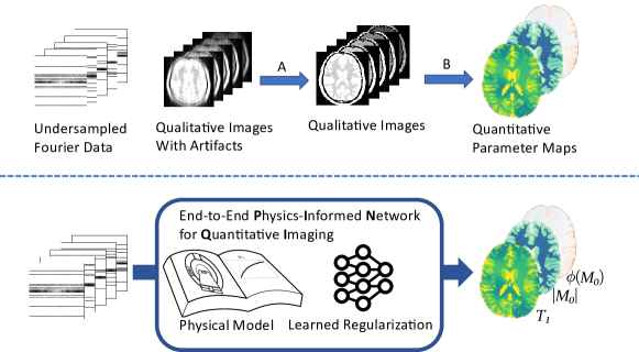
Figure 1: The problem to be solved in quantitative MRI is obtaining maps of physical parameters from undersampled measurements in Fourier space. Most previous methods consider the two steps of A) reconstructing artifact-free qualitative images and B) obtaining the parameter maps as two disjoint and independent steps (see text for details). We propose a novel end-to-end method making use of prior knowledge about the physics of data acquisition and learned regularization.

The existing data-driven approaches to solve the qMRI inverse problem, i.e. to obtain the parameter maps from the acquired k-space data, can be broadly categorized as follows. The first type of approach splits the problem into two disjoint tasks: A) image reconstruction and B) parameter regression (see fig:idea). The second type jointly solves both tasks to obtain the parameter maps directly from the k-space data. For the first task of qualitative image reconstruction, data-driven methods have made great progress: State-of-the-art results can be achieved by incorporating deep learning into an unrolled model-based reconstruction by iteratively applying a neural network as a form of learned regularization as well as enforcing consistency with the recorded k-space data and the linear signal model [9, 10, 16, 17, 18]. The second task, parameter regression, is then either carried out by classical regression using non-linear solvers [19, 20, 21, 22], dictionary matching [23], or by learned methods. Within the latter, a further distinction can be made between pixelwise mappings, such as MyoMapNet for $T_{\_}1$-mapping [14, 15] and methods using the information of multiple pixels via convolutional neural networks (CNNs), thereby implicitly learning a suitable spatial regularization [13, 12, 24]. MANTIS [13], for example, uses a UNet [25] to predict the parameter maps (originally $T_{\_}2$ maps) from qualitative magnitude images with severe undersampling artifacts. DeepT1[12], proposed for myocardial $T_{\_}1$-mapping, consists of two separate data-driven parts. First, an iterative reconstruction using recurrent CNNs [17] and data-consistency layers for image reconstruction is trained to reconstruct artifact-free qualitative images. Second, a UNet is trained to predict the quantitative maps from the magnitude of the reconstructed images. However, most learning-based methods entirely ignore prior knowledge about the physics of the signal and acquisition model relating the parameters with the quantitative images or use it only during training as part of a loss function [13, 24, 26]. Few learned methods are trained in an end-to-end manner, i.e. from k-space data to parameter maps, and fully incorporate the physical model at inference time. In DAINTY [27], a UNet predicting $T_{\_}1$ is used as a regularizer in a low-rank and sparsity regularized model-based reconstruction. PGD-Net [28] unrolls a proximal gradient descent scheme with an approximated signal function, which is implemented as a pre-trained neural network and used as a differentiable proxy of the true MR fingerprinting signal function. DOPAMINE [11] unrolls a first-order gradient descent scheme that includes an implicitly learned regularizer where small residual CNNs operating on the different parameter maps are used to learn the gradient of a regularizer. Neither employs image-space regularization nor makes use of the particular form of the forward model and both only use shallow networks.

Combining the knowledge about the physics of the acquisition model by data-consistency layers with deep learning regularization has greatly improved qualitative image reconstruction [10, 16, 29]. Thus, we want to investigate a novel approach to incorporate the full knowledge of the physics of the signal model into a learned qMRI reconstruction, while employing learned regularization in image- and parameter-space.

1.1 Our Contributions

Our main contributions to the field of deep-learning-based quantitative imaging consist of

• Introduction of non-linear optimization as a differentiable layer into qMRI reconstruction.

• A novel and general end-to-end Physics-Informed Network for Quantitative Imaging, PINQI, based on unrolled half quadratic splitting and differentiable optimization.

• Validation of the proposed approach on the task of $T_{\_}1$-mapping. We show the transferability of the network trained solely on synthetic data to in-vivo measurements.

We also demonstrate the usage of implicit differentiation for efficient evaluation of gradients with respect to all inputs of the commonly data-consistency layers of linear inverse problems as well as the non-linear optimization layer.

2 Methology

First, we introduce the notation and formulate the inverse problem to be solved in quantitative imaging. Next, we give a short introduction to differentiable optimization. We present implicit differentiation as a technique to obtain the Jacobian of solutions of optimization problems with respect to the parameters of the problems. Finally, we introduce our proposed PINQI solution to the quantitative imaging problem using differentiable optimization.

2.1 Problem Statement

By ${\bm{p}}({\bm{r}})=\left[p_{\_}1({\bm{r}}),\ldots,p_{\_}{N_{\_}P}({\bm{r}})\right]^{\mkern-1.5mu\scaleobj{0.7}{\mathsf{T}}}$ we denote for each location ${\bm{r}}$ the $N_{\_}P$ relevant physical parameters to be determined, such as relaxation times. For notational brevity, we will write ${\bm{p}}\in\mathbb{R}^{N_{\_}p\cdot N}$ for the vector representation of the parameters at $N=N_{\_}x\cdot N_{\_}y$ discrete 2D positions. In qMRI, one considers the forward model given by

$${\bm{k}}=\left(\mathbf{A}\circ q\right)\left({\bm{p}}\right)+{\bm{e}},$$ (1)

where ${\bm{k}}\in\mathbb{C}^{N_{\_}r\cdot N_{\_}c\cdot N_{\_}k}$ is the vector of recorded k-space data, $\mathbf{A}$ is a linear acquisition operator, $q$ a (non-linear) signal model, and ${\bm{e}}$ random noise. As the acquisition is performed $N_{\_}r$ times with different sampling parameters and changes in the MR sequence influencing the signal model, the forward model is given by $\mathbf{A}\circ q:\,\mathbb{R}^{N_{\_}p\cdot N}\rightarrow\mathbb{C}^{N_{\_}r\cdot N_{\_}c\cdot N_{\_}k}$ with ${\bm{p}}\mapsto[\left(\mathbf{A}_{\_}1\circ q_{\_}1\right)\left({\bm{p}}\right)^{\mkern-1.5mu\scaleobj{0.7}{\mathsf{T}}},\ldots,\left(\mathbf{A}_{\_}{N_{\_}r}\circ q_{\_}{N_{\_}r}\right)\left({\bm{p}}\right)^{\mkern-1.5mu\scaleobj{0.7}{\mathsf{T}}}]^{\mkern-1.5mu\scaleobj{0.7}{\mathsf{T}}}$. Here, the encoding operators at each acquisition $\mathbf{A}_{\_}i:\,\mathbb{C}^{N}\rightarrow\mathbb{C}^{N_{\_}c\cdot N_{\_}k}$ typically are undersampled Fourier operators. These can be written as $\mathbf{A}_{\_}i=\mathbf{S}_{\_}i\mathbf{F}\mathbf{C}$ with $\mathbf{F}$ a being two-dimensional Fourier transform and $\mathbf{S}_{\_}i$ undersampling operators, masking out all but $N_{\_}k$ discrete points in k-space. The undersampling masks are typically varied between different acquisitions. For $N_{\_}c$ receiver coils acquiring data in parallel, the coil sensitivity operator $\mathbf{C}$ expands each image to $N_{\_}c$ different views acquired by the receiver coils by pixelwise multiplying with their respective spatially varying complex-valued sensitivity maps ${\bm{c}}_{\_}c\in\mathbb{C}^{N}$, often normalized such that for each pixel $\sum_{\_}i^{N_{\_}c}|c_{\_}{i}|^{2}=1$.

A qMRI reconstruction aims to obtain the tissue parameters ${\bm{p}}$ from the acquired data ${\bm{k}}$. For uncorrelated Gaussian noise ${\bm{e}}$, the maximum likelihood estimate is

$${\bm{p^{*}}}=\operatorname*{arg\,min}_{\_}{\bm{p}}\|\mathbf{A}q\left({\bm{p}}\right)-{\bm{k}}\|^{2}\,.$$ (2)

As the inverse problem of obtaining ${\bm{p^{*}}}$ is typically ill-posed, instead the regularized problem

$$\min_{\_}{\bm{p}}\|\mathbf{A}q\left({\bm{p}}\right)-{\bm{k}}\|^{2}+\mathcal{R}({\bm{p}})$$ (3)

with a regularizer $\mathcal{R}$ has to be considered.

2.2 Differentiable Optimization

In many computer vision tasks, data-driven approaches with differentiable layers solving an inner optimization problem within a larger neural network have been used successfully [30, 31, 32]. Yet so far, in medical imaging, optimization of an inner problem is mainly only used as data-consistency layers in unrolled reconstruction networks [10] for linear problems or in deep equilibrium models. These formulate a fix-point problem that is solved by a layer of the network during the forward pass and have found some adaption in medical imaging to solve the linear MR reconstruction problem [33, 34]. In general, to incorporate optimization problems as a layer into a larger network, which can then be trained end-to-end with gradient descent algorithms, the gradients of the solution of the inner problem with respect to the inputs must be calculated. For data-consistency layers in linear problems, this can, for example, be achieved by automatic differentiation through the steps performed by the inner optimizer if each operation is differentiable [9]. The downsides are 1) all intermediate results have to be kept available, significantly increasing memory requirements, and 2) algorithms for solving non-linear problems typically contain non-differentiable operations [22]. Alternatively, for linear problems, the gradient of the output with respect to the previous solution estimate can be efficiently calculated with matrix calculus [10, 35]. A more general approach to obtain gradients through an optimization layer uses a technique known as implicit differentiation [36]. We first revise the concept before applying it in sec:backward.

Let $\mathcal{F}_{\_}{{\bm{\alpha}}}:\mathbb{R}^{n}\rightarrow\mathbb{R}$ be the twice continuously differentiable objective of the inner optimization problem solved by the layer, ${\bm{\alpha}}\in\mathbb{R}^{p}$ the parameters to backpropagate the gradient for and ${\bm{f}}:\mathbb{R}^{p}\times\mathbb{R}^{n}\rightarrow\mathbb{R}^{n}$ with ${\bm{f}}({\bm{\alpha}},{\bm{x}})=\nabla_{\_}x\mathcal{F}_{\_}{{\bm{\alpha}}}({\bm{x}})$ be the gradient of the objective function. For some ${\bm{x^{*}}}\in\mathbb{R}^{n}$ to be a minimizer of $\mathcal{F}$, the condition

$${\bm{0}}={\bm{f}}\left({\bm{\alpha}},{\bm{x^{*}}}({\bm{\alpha}})\right)$$ (4)

has to be fulfilled. The well-known implicit function theorem (IFT) in a suitable notation [37, 38] states:

Theorem 1 (Implicit Function Theorem)

Let ${\bm{f}}:\mathbb{R}^{p}\times\mathbb{R}^{n}\rightarrow\mathbb{R}^{n}$ be a continuous differentiable function, ${\bm{\alpha_{\_}0}}\in\mathbb{R}^{p}$ and ${\bm{x_{\_}0}}\in\mathbb{R}^{n}$ such that ${\bm{f}}({\bm{\alpha_{\_}0}},{\bm{x_{\_}0}})={\bm{0}}$ with non singular Jacobian $\partialderivative{{\bm{f}}}{{\bm{x}}}\left({\bm{\alpha_{\_}0}},{\bm{x_{\_}0}}\right)\in\mathbb{R}^{n\times n}$. Then, there exist an open set $S\subset\mathbb{R}^{n}$ with ${\bm{\alpha_{\_}0}}\in S$ and a unique continuously differentiable function ${\bm{x^{*}}}:S\rightarrow\mathbb{R}^{n}$ such that ${\bm{x^{*}}}({\bm{\alpha_{\_}0}})={\bm{x_{\_}0}}$ and ${\bm{f}}({\bm{\alpha}},{\bm{x^{*}}}({\bm{\alpha}}))={\bm{0}}$ for all ${\bm{\alpha}}\in S$.

Hence, eq:appoptimalcondition implicitly defines the minimizer ${\bm{x^{*}}}$ as a function of ${\bm{\alpha}}$. Differentiating both sides of eq:appoptimalcondition yields

$${\bm{0}} =\partialderivative{{\bm{f}}({\bm{\alpha}},{\bm{x^{*}}}({\bm{\alpha}}))}{{\bm{\alpha}}}=\partialderivative{{\bm{f}}}{{\bm{x^{*}}}}\partialderivative{{\bm{x^{*}}}({\bm{\alpha}})}{{\bm{\alpha}}}+\partialderivative{{\bm{f}}}{{\bm{\alpha}}}\,,$$ (5)

where ${\bm{x^{*}}}$ without explicit dependency on ${\bm{\alpha}}$ it is treated as a fixed value. By rearranging we obtain an expression for the Jacobian of the solution mapping, i.e

$$\partialderivative{{\bm{x^{*}}}({\bm{\alpha}})}{{\bm{\alpha}}} =-\left(\partialderivative{{\bm{f}}}{{\bm{x^{*}}}}\right)^{-1}\partialderivative{{\bm{f}}}{{\bm{\alpha}}}\,.$$ (6)

Therefore, by the chain rule, given the gradient of an outer loss $\partialderivative{\mathcal{L}}{{\bm{x}}}$ as a row vector at ${\bm{x}}={\bm{x^{*}}}$, the row vector $\partialderivative{L}{{\bm{\alpha}}}$ at ${\bm{\alpha}}={\bm{\alpha_{\_}0}}$ can be written as

$$\partialderivative{\mathcal{L}}{{\bm{\alpha}}}\/({\bm{\alpha_{\_}0}})=\partialderivative{\mathcal{L}}{{\bm{x}}}\/({\bm{x^{*}}})\partialderivative{{\bm{x^{*}}}({\bm{\alpha}})}{{\bm{\alpha}}}\/({\bm{\alpha_{\_}0}},{\bm{x^{*}}})$$ (7)

$$=-\partialderivative{\mathcal{L}}{{\bm{x}}}\/({\bm{x^{*}}})\left(\partialderivative{\mathcal{F}}{{\bm{x}}}{{\bm{x}}^{\mkern-1.5mu\scaleobj{0.7}{\mathsf{T}}}}\/({\bm{\alpha_{\_}0}},{\bm{x^{*}}})\right)^{-1}\partialderivative{\mathcal{F}}{{\bm{\alpha}}}{{\bm{x}}}\/({\bm{\alpha_{\_}0}},{\bm{x^{*}}})\,.$$ (8)

Finally, dropping the explicit points of evaluation in the notation, we obtain the column vector

$$\left(\partialderivative{\mathcal{L}}{{\bm{\alpha}}}\right)^{\mkern-1.5mu\scaleobj{0.7}{\mathsf{T}}} =-\partialderivative{\mathcal{F}}{{\bm{\alpha}}}{{\bm{x}}}\left(\partialderivative{\mathcal{F}}{{\bm{x}}}{{\bm{x}}^{\mkern-1.5mu\scaleobj{0.7}{\mathsf{T}}}}\right)^{-1}\left(\partialderivative{L}{{\bm{x}}}\right)^{\mkern-1.5mu\scaleobj{0.7}{\mathsf{T}}}\,,$$ (9)

where we have used the symmetry of the Hessian $\partialderivative{\mathcal{F}}{{\bm{x}}}{{\bm{x}}^{\mkern-1.5mu\scaleobj{0.7}{\mathsf{T}}}}$.

This gives the general blueprint to implement the backpropagation step for optimization layers in deep-learning frameworks. Either the analytical Hessian or the vector-Hessian-product functionality of the framework can be used in conjunction with an iterative solver for linear problems to approximately obtain $(\partialderivative{\mathcal{F}}{{\bm{x}}}{{\bm{x}}^{\mkern-1.5mu\scaleobj{0.7}{\mathsf{T}}}})^{-1}\left(\partialderivative{\mathcal{L}}{{\bm{x}}}\right)^{\mkern-1.5mu\scaleobj{0.7}{\mathsf{T}}}$ in eq:implicitdiff. For an approximate solution with an error with norm $\epsilon$, it has been shown that the error of the estimated gradient is $\mathcal{O}(\epsilon)$ [39]. The derivative with respect to the parameters of the gradient of the inner optimization loss used in eq:implicitdiff, $\partialderivative{\mathcal{F}}{{\bm{\alpha}}}{{\bm{x}}}$, can also either be calculated analytically or by autograd functionality.

2.3 Proposed Reconstruction Network PINQI

For solving the qMRI inverse problem, we propose the following, physics-informed end-to-end approach PINQI: First, we choose the regularization in eq:problem such that the objective is finding

$${\bm{p}}^{*}=\operatorname*{arg\,min}_{\_}{{\bm{p}}}\|\mathbf{A}q({\bm{p}})-{\bm{k}}\|_{\_}2^{2}+\lambda_{\_}{\tilde{p}}\|{\bm{p}}-{\bm{p}}_{\_}{\mathrm{reg}}\|_{\_}2^{2}\,,$$ (10)

with ${\bm{p}}_{\_}{\mathrm{reg}}$ a regularizing prediction for the parameters. We introduce an auxiliary variable ${\bm{y}}:=q({\bm{p}})$ and include equality by a quadratic penalty constraint as well as an additional regularization on the images,

$$\min_{\_}{{\bm{y}},{\bm{p}}} \|\mathbf{A}{\bm{y}}-{\bm{k}}\|_{\_}2^{2}+\lambda_{\_}{\tilde{p}}\left\|{\bm{p}}-{\bm{p}}_{\_}{\mathrm{reg}}\right\|_{\_}2^{2}$$ (11)

$$+\lambda_{\_}q\|q({\bm{p}})-{\bm{y}}\|_{\_}2^{2}+\lambda_{\_}y\|{\bm{y}}-{\bm{y}}_{\_}{\mathrm{reg}}\|_{\_}2^{2}\,,$$

where all $\lambda$ are positive regularization strengths. Next, we split Problem (11) into two subproblems which we solve in an alternating fashion [40] within our unrolled reconstruction network.

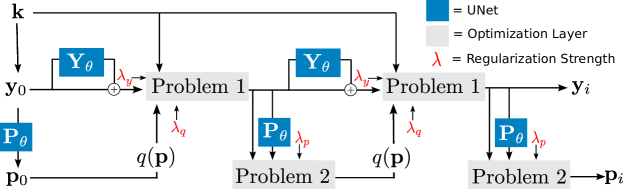
Figure 2: Schematic of the unrolled physics-informed network to solve eq:regproblem by quadratic splitting as used by our proposed PINQI. We alternate between solving two subproblems, Problem 1 is a linear data-consistency problem and solved by a differentiable conjugate-gradient block. Subproblem 2 is solved by a differentiable non-linear optimization block. $\mathbf{Y}_{\_}\theta$ denotes a residual UNet operating on qualitative images, $\mathbf{P}_{\_}\theta$ the parameter prediction UNet. The predictions of these subnetworks are used as regularizers with (learnable) strength $\lambda_{\_}y$ and $\lambda_{\_}p$, respectively. Consistency between both subproblems is relaxed to a quadratic penalty weighted by $\lambda_{\_}q$. For more details regarding the formulations of the two subproblems, see the main text.

2.3.1 Linear Subproblem: Optimization in $\mathbf{y}$

The subproblem of obtaining artifact-free qualitative images

$${\bm{y}}^{*}=\operatorname*{arg\,min}_{\_}{{\bm{y}}}\|\mathbf{A}{\bm{y}}-{\bm{k}}\|_{\_}2^{2} +\lambda_{\_}y\|{\bm{y}}-{\bm{y}}_{\_}\mathrm{reg}\|_{\_}2^{2}$$ (12)

$$+\lambda_{\_}q\|q({\bm{p}})-{\bm{y}}\|_{\_}2^{2}$$

is similar to the problem commonly solved in MR image reconstruction networks [10] by the data-consistency blocks, but extended by the model-based [6, 7, 8] last term which penalizes a discrepancy between reconstructed qualitative images and predictions based on the estimate for the quantitative parameters. As we consider multi-coil imaging, the minimizer of eq:sublinearF does not have a closed-form analytical solution. Instead, we solve a problem of the form $\mathbf{H}{{\bm{x}}}={\bm{b}}$ with $\mathbf{H}=\mathbf{A}^{{\scaleobj{0.7}{\mathsf{H}}}}\mathbf{A}+(\lambda_{\_}q+\lambda_{\_}y)\,\mathbf{I}_{\_}{N}$ and ${\bm{b}}=\mathbf{A}^{\scaleobj{0.7}{\mathsf{H}}}{\bm{k}}+\lambda_{\_}q\,q({\bm{p}})+\lambda_{\_}y\,{\bm{y}}_{\_}\mathrm{reg}$ approximately, for example with the conjugate gradient (CG) algorithm [22].

2.3.2 Non-Linear Subproblem: Optimization in $\mathbf{p}$

By introducing $\lambda_{\_}p=\nicefrac{{\lambda_{\_}{\tilde{p}}}}{{\lambda_{\_}q}}$, the second subproblem can be written as finding

$${\bm{p^{*}}}=\operatorname*{arg\,min}_{\_}{{\bm{p}}}\|q({\bm{p}})-{\bm{y}}\|_{\_}2^{2}+\lambda_{\_}p\left\|{\bm{p}}-{\bm{p}}_{\_}{\mathrm{reg}}\right\|_{\_}2^{2}\,.$$ (13)

Due to the non-linear signal function $q$, this subproblem is non-linear. Hence, we introduce the non-linear optimization layer depicted in fig:nonlinearlayer. This layer uses L-BFGS [21, 22] to approximately solve the problem in the forward pass. Depending on the concrete signal model, within this layer, different solvers and preconditioning techniques might be chosen [41] instead.

Finally, we construct our proposed PINQI as shown in fig:network by alternating between both subproblems for a fixed number of iterations. In each iteration $i=1\ldots T$, we obtain predictions for the qualitative, artifact-free images ${\bm{y}}^{i}$ and for the quantitative parameters ${\bm{p}}^{i}$. For regularization, we use predictions obtained by trained subnetworks with parameters ${\bm{\theta}}\in\mathbb{R}^{n}$ as ${\bm{y}}^{i}_{\_}\mathrm{reg}={\bm{y}}^{i}_{\_}{\theta}=\mathbf{Y}_{\_}\theta({\bm{y}}^{i-1},i)$ and ${\bm{p}}^{i}_{\_}\mathrm{reg}={\bm{p}}^{i}_{\_}{\theta}=\mathbf{P}_{\_}\theta({\bm{y}}^{i},i)$, respectively. All learnable parameters of the UNet subnetworks are shared between iterations.

2.4 Gradients of the Subproblem Solutions

We propose to train PINQI end-to-end, i.e. we construct an objective function $\mathcal{L}$ which depends on the final predicted real-valued quantitative parameter maps. Also, we aim to use gradient descent-based algorithms to optimize the learnable network weights ${\bm{\theta}}$ and use backpropagation to find the direction of the steepest descent. Thus, we need to be able to calculate the gradients of the solutions found by the solvers of both subproblems with respect to all variables depending on ${\bm{\theta}}$. We achieve this by implementing the solvers as differentiable optimization layers as presented in sec:optimization.

First, we specialize the general concept to a regularized non-linear regression problem, i.e. an inner problem of obtaining ${\bm{p^{*}}}{=}\operatorname*{arg\,min}_{\_}{{\bm{p}}}\mathcal{F}({\bm{p}})$ with an objective

$$\mathcal{F}({\bm{p}})=\|q({\bm{p}})-{\bm{y}}\|_{\_}2^{2}+\lambda\|{\bm{p}}-{\bm{p}}_{\_}\mathrm{reg}\|^{2}\,,$$ (14)

as used in subproblem 2. Suppose the gradient of the inner objective at ${\bm{x}}^{*}$ is continuously differentiable and its Jacobian is invertible. Then, the required gradient of $\mathcal{L}$ with respect to the trainable weights can simply be found by applying eq:implicitdiff. The resulting equations for the propagation of gradients to $\lambda$, ${\bm{p}}_{\_}\mathrm{reg}$ and ${\bm{y}}$ are shown in fig:nonlinearlayer, which summarizes our proposed non-linear regression layer for this subproblem. Within this layer, we use CG to approximate ${\bm{g}}$, which denotes the product of the inverse Hessian of $\mathcal{F}$ with the gradient of $\mathcal{L}$ with respect to the output of the solver. We employ automatic differentiation to compute the Hessian-vector product applied inside the CG algorithm, as well as to compute the derivative (with respect to ${\bm{\theta}}$) of the gradient (with respect to ${\bm{p}}$) of the inner loss. In sec:regressionexp we investigate the influence of including a single instance of our differentiable non-linear optimization layer at the end of an otherwise unchanged qualitative image reconstruction network.

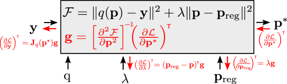
Figure 3: Proposed non-linear optimization layer, finding ${{\bm{p}}^{*}=\operatorname*{arg\,min}_{\_}{\bm{p}}\mathcal{F}}({\bm{p}})$ with an off-the-shelf solver while allowing backpropagation of the gradients (red) to the regularization parameters, $\lambda$ and ${\bm{p}}_{\_}\mathrm{reg}$, and data ${\bm{y}}$.

Similarly, backpropagation through the solver of the linear image reconstruction subproblem 1 can also be efficiently calculated, as demonstrated in [10] for gradients with respect to ${\bm{y}}_{\_}{\mathrm{reg}}$. Extending upon these results, we use implicit differentiation to derive the gradients with respect to all inputs: For an inner optimization objective of the form

$$\mathcal{F}(\vec{y})=\|\mathbf{A}{\bm{y}}-{\bm{k}}\|^{2}+\sum_{\_}i\lambda_{\_}i\|{\bm{y}}-{\bm{y}}_{\_}\mathrm{i}\|^{2}\,,$$ (15)

and a solution ${\bm{y^{*}}}\in\mathbb{C}^{N}$, that fulfills the necessary condition $\nabla F({\bm{y^{*}}})=0$, application of eq:implicitdiff and defining

$${\bm{g}}:=(\mathbf{A}^{\scaleobj{0.7}{\mathsf{H}}}\mathbf{A}+\textstyle\sum_{\_}i\lambda_{\_}i\mathbf{I}_{\_}N)^{-1}\left(\partialderivative{\mathcal{L}({\bm{y}}^{*})}{{\bm{y}}^{*H}}\right)^{\mkern-1.5mu\scaleobj{0.7}{\mathsf{T}}}$$ (16)

gives the gradients of the outer loss (in Wirtinger calculus [42]):

$$\partialderivative{\mathcal{L}}{{\bm{y}}_{\_}\mathrm{i}^{\scaleobj{0.7}{\mathsf{H}}}}=\lambda_{\_}i{\bm{g}}\,, \partialderivative{\mathcal{L}}{\lambda_{\_}i}=\Re{({\bm{y}}_{\_}i-{\bm{y}})^{\scaleobj{0.7}{\mathsf{H}}}{\bm{g}}}\,, \partialderivative{\mathcal{L}}{{\bm{k}}^{\scaleobj{0.7}{\mathsf{H}}}}=\mathbf{A}{\bm{g}}\,.$$ (17)

For multi-coil MRI, the linear operator defining the data recorded in a single acquisition by the $j$-th coil is of the form $\mathbf{A}_{\_}j=\mathbf{S}\mathbf{F}\mathbf{C}_{\_}j$, and,

$$\partialderivative{\mathcal{L}}{{\bm{c}}_{\_}j^{\scaleobj{0.7}{\mathsf{H}}}} =\left(\mathbf{F}^{\scaleobj{0.7}{\mathsf{H}}}\left(\mathbf{A}_{\_}j{\bm{y^{*}}}-{\bm{k}}_{\_}j\right)\right)\odot\overline{{\bm{g}}}+\left(\mathbf{F}^{\scaleobj{0.7}{\mathsf{H}}}\mathbf{A}_{\_}j{\bm{g}}\right)\odot\overline{{\bm{y}}}^{*}$$ (18)

can be used to backpropagate the gradient of the outer loss to the $j$-th estimated unnormalized sensitivity map ${\bm{c}}_{\_}j$. Here $\odot$ denotes the Hadamard product, $\overline{{\bm{g}}}$ the complex conjugate of ${\bm{g}}$, and ${\bm{k}}_{\_}j$ the data recorded by the $j$-th coil.

3 Application to $T_{\_}1$-Mapping

The proposed PINQI can be used for many quantitative MR imaging techniques by adapting $q$ to the respective signal model and $\mathbf{A}$ to the acquisition operator.
For our experiments, we chose a $T_{\_}1$-mapping of the brain using a saturation recovery sequence as a typical, yet conceptually simple, qMRI problem. Here, the signal model $q_{\_}i$ at the $i$-th acquisition is given for each pixel by

$$q_{\_}i(\real\,M_{\_}0,\imaginary\,M_{\_}0,T_{\_}1)=M_{\_}0(1-\exp(-\tau_{\_}i/T_{\_}1))$$ (19)

with $\mathrm{Re}\,M_{\_}0$ and $\mathrm{Im}\,M_{\_}0$ denoting the real and imaginary part of the complex initial magnetization $M_{\_}0$, $T_{\_}1$ the longitudinal relaxation time, and $\tau_{\_}i$ the $i$-th saturation recovery time, i.e. the delay between the magnetization preparation pulse and the data acquisition. As encoding operator $\mathbf{A}$, we chose a Fourier transform with Cartesian sampling, $8$-fold undersampling, and 8 receiver coils.

All code relating to PINQI, trained weights, our implementations of the reference methods, the synthetic data generation as well as the MR sequences will be made available after peer-review at github.com/fzimmermann89/PINQI.

3.1 Training Dataset and Data Aquisition

We utilized synthetic data for training and validation and conducted testing on both synthetic data and real scanner data.

3.1.1 Synthetic Data

The synthetic data was generated from the BrainWeb dataset [43], which consists of three-dimensional segmentation masks of 20 healthy human brains, which we split into 16/1/3 for training/validation/testing. During the training process, we randomly assigned anatomically plausible values[20] for $M_{\_}0$ and $T_{\_}1$ to each of the 11 tissue classes in every sample on-the-fly. These values were combined with axial slices of the masks, resampled to $192\times 192$ pixels, into initial synthetic parameter maps. To increase spatial variability and prevent overfitting to piecewise constant images, we augmented the $T_{\_}1$-maps by multiplying them with low-variance 2D polynomials. Similarly, we augmented the $M_{\_}0$-maps by a random spatially slowly varying complex phase and bias field. As additional augmentations during training, we performed flips and rotations $<$10°. The resulting parameter maps were considered ground truth labels. In addition, we generated sample-specific masks indicating the presence of brain tissue within the maps. During training, these masks were used to weigh down the losses outside the brain region. During the testing phase, all quantitative measures used to report the performance of the methods were restricted to the relevant brain tissue.

The saturation recovery times were set as either 0.5 s, 1 s, 1.5 s, 2 s, and 8 s, or as 0.5 s, 0.7 s, 0.9 s, 1.1 s, 1.3 s, 1.6 s, 2 s, and 8 s for the ablation study. We used variable density 1D-under-sampling with 8 simulated bird-cage-like receiver coils with random orientation. The undersampling patterns were randomly chosen for each recovery time and for each sample. Finally, for each sample, we added complex Gaussian noise with randomly chosen standard variation $\sigma\in(0.001,0.04)$ to simulate noisy measurements.

Our synthetic validation and testing datasets consisted of a fixed set of generated labels and simulated noisy undersampled k-space measurements.

3.1.2 Data Aquisition

For further validation of our proposed method, we acquired two sets of scanner data on a $3$ T MRI system (Siemens Verio): 1) data from a physical phantom and 2) data from the brains of healthy volunteers. The examination was approved by the local ethics committee and is in accordance with the relevant guidelines and regulations. Written informed consent was received from all subjects prior to the examination. The phantom consisted of 9 tubes filled with liquids prepared to have $T_{\_}1$ times in the range of approx. $250$ ms-$1750$ ms. We used adiabatic saturation pulses, 5 saturation recovery times, spoiled GRE readouts with inside-out order and $1$ mm$\times 1$ mm$\times 8$ mm resolution, $192\times 192$ matrix size, $6\deg$ flip angle, a 32-channel head coil. For each saturation time, the 1D Cartesian undersampling was chosen randomly, analogously to our training. As a reference, we performed fully sampled saturation recovery measurements with $18$ delay times and obtained the $T_{\_}1$ values by pixel-wise regression on the reconstructed images. Coil sensitivity maps were estimated from the fully sampled image with the longest $\tau$ [44]. All MR sequences were implemented using the vendor-agnostic Pulseq framework [45].

3.2 PINQI: Implementation Details

We set the number of alternations between the subproblems in our implementation of PINQI as $T=5$ (empirically chosen). In the non-linear subproblem, we used the L-BFGS algorithm[21, 22] with a trigonometric transformation of the variables [41] to enforce the bounds $\real(M_{\_}0)\in(-2,2)$, $\imaginary(M_{\_}0)\in(-2,2)$, and $R_{\_}1:=1/T_{\_}1\in(-1s^{-1},20s^{-1})$. These bounds are much wider than any plausible predictions and only served to increase stability at the beginning of training.

Both regularizing networks, $\mathbf{P}_{\_}{\bm{\theta}}$ and $\mathbf{Y}_{\_}{\bm{\theta}}$, are UNets [25] with residual blocks, each consisting of two SiLU[46] activated convolutions (window size 3) and group normalizations (group size 16)[47]. In $\mathbf{Y}_{\_}{\bm{\theta}}$, the two convolutions of each block handle all temporal points as batched samples, and a third convolution operates along the temporal direction, handling all spatial points as batched samples [48]. In both UNets, we condition on the iteration of the unrolled reconstruction by performing learned projections to scale and shift values for each feature map [49] after the first convolution in each encoder and decoder block. The downscaling in the UNet is done with stride 2, kernel 2 max-pooling operations in the spatial dimensions. Each upscaling is performed with 2x bilinear interpolation in the spatial dimensions followed by a 3x3 convolution. The number of output features at the different layers in $\mathbf{Y}_{\_}{\bm{\theta}}$ is empirically chosen as (16, 32, 48, 64), and as (32, 64, 96, 128) in $\mathbf{P}_{\_}{\bm{\theta}}$. This results in 597,323 and 2,235,308 learnable weights, respectively. We found initializing the network such that each block mainly operates pixel-wise [50] improved training stability.

All regularization strengths $\lambda_{\_}{p,i}$, $\lambda_{\_}{y,i}$, and $\lambda_{\_}{q,i}$ are iteration-dependent learnable parameters. We enforced the positivity of these parameters by setting $\lambda_{\_}{i}=\log\frac{1}{5}(1+\exp\{5\tilde{\lambda_{\_}i}\})$ and optimizing for each $\tilde{\lambda}_{\_}i$. We empirically chose an initialization corrosponding to $\lambda_{\_}{p,i}=3$, $\lambda_{\_}{y,i}=0.1$, and $\lambda_{\_}{q,i}=0.1+0.05i$. The training was performed by minimizing the MSE between the predicted quantitative parameters, $R_{\_}1=1/T_{\_}1$, $\real(M_{\_}0),\imaginary(M_{\_}0)$, and the corresponding target parameters. Deep supervision [51, 52] was applied by also incorporating the MSE loss of the predicted parameters during all previous iterations, strongly weighted down by a factor of $0.05$. We pretrained $\mathbf{P}_{\_}{\bm{\theta}}$ for one epoch with random linear interpolation between the zero-filled reconstructions of the noisy k-space data and the ground truth (noise- and artifact-free) qualitative images as input with MSE loss on the estimated parameters. The training was performed for 80 epochs. Both training phases were performed using the Adam optimizer [53] with a maximum learning rate $0.004$ for the UNet parameters and $0.001$ for all $\bar{\lambda}$’s, a linear warmup and cosine learning rate schedule [54], weight decay [55] $0.01$, and a batch size of 16.

$T_{\_}1$                                                $|M_{\_}0|$

Figure 4: Examplary results of the different methods for one simulated measurement from the test dataset. More details regarding the different methods are provided in the text. For each method, the magnitude of $M_{\_}0$ and deviation from the ground truth are shown in the top two rows. The calculated $T_{\_}1$ and deviation from ground truth are shown in the bottom two rows.

3.3 Method of Comparison

Besides our proposed PINQI approach, we provide results of our implementations of three recently published learned reconstruction methods trained and tested on the same dataset. As the general superiority of the selected learned comparison methods to non-learned methods has been established by the respective authors [12, 11, 13, 10], we abstain from comparing against non-learned baselines.

DeepT1 [12]

Our reimplementation of DeepT1 tries to stay as close as possible to the provided description in the original publication while adapting to our synthetic data and the saturation recovery signal model. The task of magnitude-only image reconstruction by an unrolled reconstruction uses a recurrent CNN (297,538 learnable weights). We replaced the original data-consistency layers, which were only suitable for a single coil setting, with CG-based ones. The parameter estimation from the reconstructed magnitude images was done with a UNet (20,547,906 learnable weights).

MANTIS [13]

We adopted the MANTIS method for $T_{\_}1$-mapping and training on our simulated dataset. As MANTIS takes zero-filled magnitude images as input, it cannot predict the phase of $M_{\_}0$. The particular UNet architecture proposed for MANTIS uses 29,248,258 learnable parameters. We used the proposed combination of the MSE of the quantitative parameters and in k-space as loss and tried different weighting of the latter. Although we noticed only a minimal influence on the performance on the validation set, we report results for a network trained with the optimal weighting found in our experiments of $0.01$.

DOPAMINE [11]

We modified the DOPAMINE method for our signal model and supervised training. Our implementation performs 10 iterations of unrolled gradient descent. Each overall stepsize and each weighting of the neural network predicted step were scalar trainable parameters with softplus enforced positivity. The two regularizing CNNs and the network for starting point prediction combined had 317,894 trainable parameters in total. The training was performed on MSE of ${\bm{p}}$. As the training was highly unstable, we slightly modified DOPAMINE by soft-clipping each update in the unrolled gradient descent via a scaled $\tanh$. A clipping threshold higher than the parameters’ dynamic range over the training data was sufficient to stabilize training. We emphasize that during inference on the validation set, each update step proposed by the network was much smaller than allowed by the clipping, thus our modification should not negatively influence test performance.

3.4 Ablation Study

Ablations of different parts of our proposed unrolled network are used to show the incremental benefits of the major components of our method. For each ablation, the respective learning rate of the parameters of the UNet was tuned based on the validation set MSE. The study was performed for eight acquisition times.

Unrolled Reconstruction Utilizing Knowledge of the Non-Linear Signal Model

To show the benefit of our proposed unrolling scheme, we consider, similar to DeepT1, solving the two problems of image reconstruction and parameter estimation only once. We use an unrolled model-based image reconstruction with a UNet-predicted regularization (5 iterations of network application and data-consistency) [10, 9]. Parameters are predicted by a separate UNet. Both UNets have the same architecture as the corresponding ones in PINQI. We performed a pretraining of the reconstruction network for 5 epochs (optimizing on MSE of the complex-valued qualitative images) followed by an end-to-end optimization for 60 epochs. This baseline approach does not use the non-linear signal model $q$ at inference time but benefits from architectural improvements to the CNNs over the comparison methods and end-to-end training.

Image-Space Regularization

We set $\lambda_{\_}y=0$ and remove $\mathbf{Y}_{\_}\theta$ from PINQI, eliminating the learned regularization in image-space while retaining the regularization in the non-linear subproblem. The training set-up and all other parameters are kept the same.

Parameter-Space Regularization

We set $\lambda_{\_}p=0$ and remove $\mathbf{P}_{\_}\theta$ from PINQI, effectively removing the learned regularization in parameter-space. Instead, we only perform a non-regularized regression on the signal model in subproblem 2. All other parameters remain unchanged.

Differentiable Non-Linear Solver

We remove the non-linear optimization block for subproblem 2 from our network and instead directly consider the network prediction of the parameters as the solution of the subproblem. Note that we still iterate between the subproblems and train end-to-end.

Repeated UNet Application

We only apply the image-space and parameter-space UNets once, i.e. ${\bm{p}}_{\_}\mathrm{reg}=\mathbf{P}_{\_}\theta({\bm{y}}_{\_}0)$ and ${\bm{y}}_{\_}\mathrm{reg}=\mathbf{Y}_{\_}\theta({\bm{y}}_{\_}0)$, instead of updating the predictions in each iteration of the unrolled reconstruction. While the number of training parameters stays constant, this significantly reduces the computation necessary in a single forward pass.

For further investigation of the advantage of incorporating differentiable non-linear regression into the reconstruction, we used the same UNet architecture as used in PINQI for $\mathbf{Y}_{\_}\theta$ also in an unrolled reconstruction of the qualitative images ${\bm{y}}$ and compare the following two cases:

Neural Network Reconstruction and Separate Regression

We optimized the network by minimizing the MSE of the qualitative images. At inference time, we used the resulting reconstructed images to perform a non-linear least-squares regression using BFGS to obtain ${\bm{p}}$.

Neural Network with Non-linear Optimization Layer

We include the non-linear regression by means of the proposed optimization layer (fig:nonlinearlayer in the network. As a result, we were able to train the network in an end-to-end fashion, minimizing the MSE of the quantitative parameters.

4 Results

4.1 Comparison with Reference Methods

The results of training PINQI and the comparison methods on the synthetic dataset and application on the test set are shown in fig:resultsilicobox. Our proposed PINQI method achieves a normalized root mean squared error (nRMSE) of the $T_{\_}1$ maps of less than $0.10$ whereas the lowest nRMSE achieved by one of the comparison methods is $0.13$ (DeepT1) and both MANTIS and DOPAMINE have nRMSE exceeding $0.2$. The mean absolute error (MAE) of $T_{\_}1$ is again lowest for PINQI ($0.05$) compared to $0.07$, $0.15$, and $0.13$ for DeepT1, MANTIS, and DOPAMINE, respectively. Examples of parameter maps for $T_{\_}1$ as well as the magnitude of $M_{\_}0$ obtained for a random slice of the test dataset are shown in fig:resultsilico. Here, only PINQI was able to resolve the fine details.

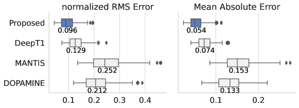
Figure 5: Comparison of our proposed PINQI with three different state-of-the-art learned qMRI reconstruction methods [13, 12, 11] in terms of nRMSE and MAE of $T_{\_}1$ for each sample of the test set. The mean values over all samples are labeled. PINQI improves upon all of the comparison methods in both metrics.

4.2 Ablation Study

The performance results obtained from the ablations are summarized in terms of nRMSE and MAE of $T_{\_}1$ in fig:ablation. The greatest increases in both MAE and nRMSE compared to the full PINQI as proposed are observed if either a) the UNets are only applied once to obtain $p_{\_}{\mathrm{reg}}$ and $y_{\_}{\mathrm{reg}}$ independent of the iteration of the unrolled scheme, or b) the parameter regularization network is completely removed. Both observations highlight the importance of learned regularization. The removal of the BFGS solver in the non-linear subproblem, corresponding to setting $\lambda_{\_}p^{i}=\infty$, resulting in ${\bm{p}}^{i}={\bm{p}}^{i}_{\_}{{}_{\_}\theta}$, also severely degrades the performance. We observed further degradation by full removal of the explicit knowledge about the signal function $q$, i.e. only using alternating between a linear problem with Fourier-space data-consistency and a parameter prediction UNet, corresponding to also setting $\lambda_{\_}q^{i}=0$. The comparison between a learned reconstruction of qualitative images with the parameter regression as a post-processing step, and the inclusion of the regression in the network with end-to-end training shows a reduction of the mean nRMSE of the $T_{\_}1$-maps of ${>}20\%$.

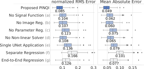
Figure 6: Results of the ablation study and reference methods for $T_{\_}1$, highlighting the importance of iteratively applying both regularizing UNets as well the inclusion of the signal function via a non-linear regression layer. Note, here $N_{\_}r=8$ and the saturation times $\tau$ differ from those used in fig:resultsilicobox. For further details, see the main text.

4.3 Phantom and In-Vivo Application

We applied the final trained network to the data acquired from the physical phantom and used the reference measurement to obtain the mean $T_{\_}1$ for each region-of-interest (ROI) for comparison. The RMS deviation between our proposed method and these reference values was 25  ms, the full results for all nine ROIs are shown in tab:phantom.

Table 1: $T_{\_}1$-values (in s) and standard deviations over ROIs obtained for the physical phantom by the fully-sampled reference method with 18 saturations delays compared to PINQI with 8-fold undersampling and 5 delays.

Reference	0.28	0.38	0.39	0.45	0.59	0.60	1.15	1.42	1.76
Std. Dev.	0.01	0.01	0.03	0.01	0.02	0.02	0.04	0.06	0.13
PINQI	0.29	0.36	0.43	0.47	0.60	0.59	1.12	1.47	1.78
Std. Dev.	0.02	0.02	0.05	0.03	0.02	0.04	0.03	0.12	0.08
Difference	4 %	-5 %	9 %	3 %	2 %	-2 %	-3 %	3 %	1 %

To qualitatively demonstrate the applicability of the proposed method to real, unseen in-vivo measurements, we present the results of the volunteer study in fig:invivo. Even though the acquisition was severely undersampled, the network predicts $T_{\_}1$-maps in agreement with the fully-sampled references and only minor artifacts remain.

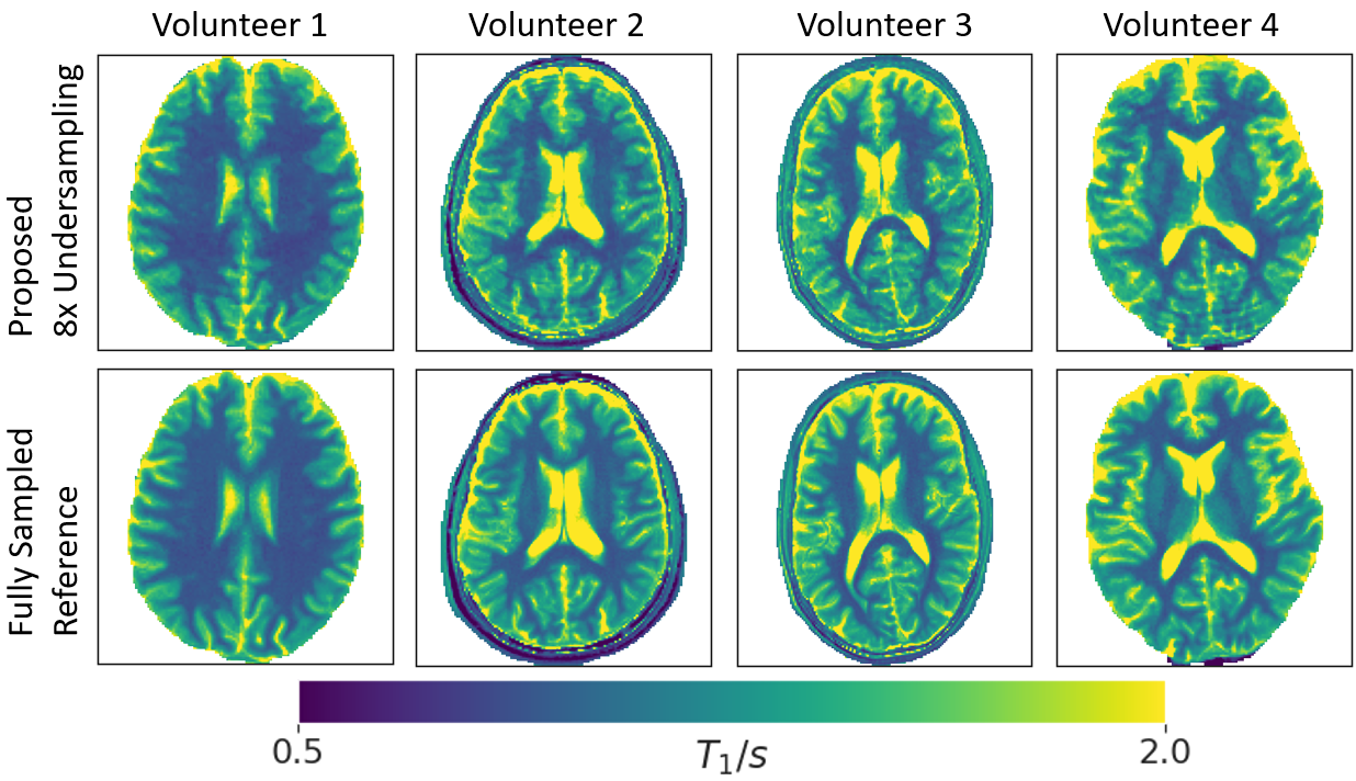
Figure 7: Examples of application of the network to 8x accelerated saturation recovery scans of the brains of four volunteers. Even though the network was trained on synthetic data only, the method is able to successfully remove most of the artifacts caused by the severe undersampling and results in $T_{\_}1$ closely matching the fully sampled saturation recovery measurements (bottom row).

5 Discussion

We have demonstrated the superiority of PINQI for saturation recovery $T_{\_}1$-mapping compared to three current state-of-the-art qMRI reconstruction techniques, as evidenced by the lower $T_{\_}1$-errors on the synthetic test dataset (fig:resultsilicobox). Given that only $T_{\_}1$ holds clinical significance among the parameters obtainable in a saturation recovery sequence, and considering that most of the compared methods do not provide access to the phase of $M_{\_}0$, our quantitative comparison here was primarily focused on $T_{\_}1$. The methods used for comparison, MANTIS, DeepT1, and DOPAMINE all have their own characteristics and limitations. MANTIS utilizes a fully learned mapping from magnitude qualitative images with artifacts to quantitative parameter maps, but only incorporates the physical model during training. DeepT1 enforces data-consistency between qualitative images and recorded k-space data, but does not enforce consistency between the final predicted parameter maps and recorded data. DOPAMINE explicitly uses knowledge about the non-linear signal model during inference, but does not employ image-space regularization and can use only shallow CNNs for parameter-space regularization due to the high number of iterations necessary. In contrast, PINQI incorporates data-consistency for the non-linear signal model through non-linear optimization layers, allowing for the inclusion of prior knowledge about the underlying physics at each iteration of the unrolled reconstruction. Additionally, PINQI makes use of both image- and parameter-space regularization and explicitly formulates the influence of all UNets as a learned regularizer. In total, these distinctions position PINQI as a unique method in qMRI reconstruction. Note that for a fair comparison, we reimplemented and adjusted the comparison methods to our dataset and signal model, as well as optimized hyperparameters rather than relying on the choices of the respective works. We were unable to use DOPAMINE as published, as training was highly unstable. We speculate, that the combination of an iteration-dependent but data-independent stepsize factor and a first-order gradient step without any thresholds was causing high susceptibility to even minor outliers. We had to modify the training to overcome this issue.

In our ablation study, we highlighted the importance of both image- and parameter-space regularization networks, as well as the utilization of the non-linear optimization layer and the signal model. Removal of any of these major components resulted in severe degradation, as summarized in fig:ablation. By employing an unrolling approach and alternating between the two subproblems, we were able to update the predictions used as learned regularizations in each iteration, which proved to be highly beneficial compared to a single application of the UNets. This suggests, that the UNets were able to make use of the gradually restored information within the unrolled algorithm. Moreover, we have demonstrated that the addition of a single non-linear optimization, as a final layer, to an otherwise unchanged learned reconstruction, can significantly reduce the error in the resulting parameter maps compared to performing a separate regression as a post-processing step outside the network (see fig:ablation, End-to-End Regression vs. Separate Regression). This approach can be seamlessly integrated into existing reconstruction methods, enabling training with an objective that aligns more closely with the true objective in quantitative MRI. Essentially, it can be viewed as a task-specific loss function, which effectively penalizes reconstruction errors of the intermediate qualitative images that contribute to poor final regression results. Unlike a simple $L_{\_}p$ loss on the qualitative intermediate images, this approach allows for more efficient learning by focusing on important features [56, 57]. We emphasize the potential of adding a single differentiable regression layer to both existing and future quantitative imaging methods as a straightforward means of incorporating knowledge about the signal model.

Finally, we demonstrated that PINQI, even when trained solely on synthetic data, can be successfully applied to real data. This was confirmed both quantitatively, with low deviations from the reference measurements of the physical phantom in tab:phantom, and qualitatively, through the reconstruction of nearly artifact-free maps from undersampled data in fig:invivo. We also note the possibility of self-supervised fine-tuning for adaptation from the assumed forward model during training to the partially unknown and potentially different true forward model during testing [58]. Similarly, the estimated coil sensitivity maps used in the linear acquisition operator could be improved by an additional subnetwork [9]. However, for the sake of simplicity and comparability, we abstained from implementing such modules in our network or in any of the comparison methods. Nevertheless, eq:csmgrad, obtained through implicit differentiation, would facilitate an efficient extension.

While we have only demonstrated the application of PINQI to Cartesian undersampled $T_{\_}1$-mapping, the splitting of PINQI can be trivially adapted to many inverse problems of the form described by eq:problem by adjusting the non-linear signal model and the linear acquisition operator. Thus, PINQI represents a general physics-informed network for many quantitative imaging inverse problems.

6 Conclusion

Our proposed method, PINQI, presents a novel approach to quantitative image reconstruction by combining unrolled optimization, differentiable optimization layers, and learned regularization to fully utilize prior knowledge regarding the underlying physics. On a representative qMRI task, $T_{\_}1$ mapping of the brain, we demonstrated superiority compared to three established data-driven reconstruction methods on a synthetic test dataset. Finally, we showed that our model, while trained on synthetic data alone, is transferable to in-vivo data.

References

- [1] K. P. Pruessmann, M. Weiger, M. B. Scheidegger, and P. Boesiger, “SENSE: Sensitivity encoding for fast MRI,” Magnetic Resonance in Medicine, vol. 42, no. 5, pp. 952–962, 1999. 10.1002/(SICI)1522-2594(199911)42:5¡952::AID-MRM16¿3.0.CO;2-S
- [2] M. Lustig, D. L. Donoho, J. M. Santos, and J. M. Pauly, “Compressed sensing mri,” IEEE Signal Processing Magazine, vol. 25, no. 2, pp. 72–82, 2008. 10.1109/MSP.2007.914728
- [3] M. Doneva, P. Börnert, H. Eggers, C. Stehning, J. Sénégas, and A. Mertins, “Compressed sensing reconstruction for magnetic resonance parameter mapping,” Magnetic Resonance in Medicine, vol. 64, no. 4, pp. 1114–1120, 2010. 10.1002/mrm.22483
- [4] X. Wang, V. Roeloffs, J. Klosowski, Z. Tan, D. Voit, M. Uecker, and J. Frahm, “Model-based T1 mapping with sparsity constraints using single-shot inversion-recovery radial FLASH,” Magnetic Resonance in Medicine, vol. 79, no. 2, pp. 730–740, 2018. 10.1002/mrm.26726
- [5] B. Zhao, F. Lam, and Z. P. Liang, “Model-based MR parameter mapping with sparsity constraints: Parameter estimation and performance bounds,” IEEE Transactions on Medical Imaging, vol. 33, no. 9, pp. 1832–1844, 2014. 10.1109/TMI.2014.2322815
- [6] K. T. Block, M. Uecker, and J. Frahm, “Undersampled radial MRI with multiple coils. Iterative image reconstruction using a total variation constraint,” Magnetic Resonance in Medicine, vol. 57, no. 6, pp. 1086–1098, 2007. 10.1002/mrm.21236
- [7] J. Tran-Gia, D. Stäb, T. Wech, D. Hahn, and H. Köstler, “Model-based Acceleration of Parameter mapping (MAP) for saturation prepared radially acquired data,” Magnetic Resonance in Medicine, vol. 70, no. 6, pp. 1524–1534, 2013. 10.1002/mrm.24600
- [8] K. M. Becker, J. Schulz-Menger, T. Schaeffter, and C. Kolbitsch, “Simultaneous high-resolution cardiac T1 mapping and cine imaging using model-based iterative image reconstruction,” Magnetic Resonance in Medicine, vol. 81, no. 2, pp. 1080–1091, 2019. 10.1002/mrm.27474
- [9] A. Sriram, J. Zbontar, T. Murrell, A. Defazio, C. L. Zitnick, N. Yakubova, F. Knoll, and P. Johnson, “End-to-End Variational Networks for Accelerated MRI Reconstruction,” in Medical Image Computing and Computer Assisted Intervention – MICCAI 2020. Lecture Notes in Computer Science, vol. 12262 LNCS, 2020. 10.1007/978-3-030-59713-9_7. ISBN 9783030597122. ISSN 16113349 pp. 64–73.
- [10] H. K. Aggarwal, M. P. Mani, and M. Jacob, “MoDL: Model-Based Deep Learning Architecture for Inverse Problems,” IEEE Transactions on Medical Imaging, vol. 38, no. 2, pp. 394–405, 2019. 10.1109/TMI.2018.2865356
- [11] Y. Jun, H. Shin, T. Eo, T. Kim, and D. Hwang, “Deep model-based magnetic resonance parameter mapping network (DOPAMINE) for fast T1 mapping using variable flip angle method,” Medical Image Analysis, vol. 70, p. 102017, 2021. 10.1016/j.media.2021.102017
- [12] H. Jeelani, Y. Yang, R. Zhou, C. M. Kramer, M. Salerno, and D. S. Weller, “A Myocardial T1-Mapping Framework with Recurrent and U-Net Convolutional Neural Networks,” Proceedings - International Symposium on Biomedical Imaging, vol. 2020-April, pp. 1941–1944, 2020. 10.1109/ISBI45749.2020.9098459
- [13] F. Liu, L. Feng, and R. Kijowski, “MANTIS: Model-Augmented Neural neTwork with Incoherent k-space Sampling for efficient MR parameter mapping,” Magnetic Resonance in Medicine, vol. 82, no. 1, pp. 174–188, 2019. 10.1002/mrm.27707
- [14] R. Guo, H. El-Rewaidy, S. Assana, X. Cai, A. Amyar, K. Chow, X. Bi, T. Yankama, J. Cirillo, P. Pierce, B. Goddu, L. Ngo, and R. Nezafat, “Accelerated cardiac T1 mapping in four heartbeats with inline MyoMapNet: a deep learning-based T1 estimation approach,” Journal of Cardiovascular Magnetic Resonance, vol. 24, no. 1, pp. 1–15, 2022. 10.1186/s12968-021-00834-0
- [15] O. Cohen, B. Zhu, and M. S. Rosen, “MR fingerprinting Deep RecOnstruction NEtwork (DRONE),” Magnetic Resonance in Medicine, vol. 80, no. 3, pp. 885–894, 2018. 10.1002/mrm.27198
- [16] J. Schlemper, J. Caballero, J. V. Hajnal, A. N. Price, and D. Rueckert, “A Deep Cascade of Convolutional Neural Networks for Dynamic MR Image Reconstruction,” IEEE Transactions on Medical Imaging, vol. 37, no. 2, pp. 491–503, 2018. 10.1007/978-3-319-59050-951
- [17] C. Qin, J. Schlemper, J. Caballero, A. N. Price, J. V. Hajnal, and D. Rueckert, “Convolutional recurrent neural networks for dynamic MR image reconstruction,” IEEE Transactions on Medical Imaging, vol. 38, no. 1, pp. 280–290, 2019. 10.1109/TMI.2018.2863670
- [18] Y. Yang, J. Sun, H. Li, and Z. Xu, “Deep ADMM-Net for compressive sensing MRI,” Advances in Neural Information Processing Systems, vol. 29, 2016. 10.5555/3157096.3157098
- [19] K. Chow, J. A. Flewitt, J. D. Green, J. J. Pagano, M. G. Friedrich, and R. B. Thompson, “Saturation recovery single-shot acquisition (SASHA) for myocardial T 1 mapping,” Magnetic Resonance in Medicine, vol. 71, no. 6, pp. 2082–2095, 2014. 10.1002/mrm.24878
- [20] J. Z. Bojorquez, S. Bricq, C. Acquitter, F. Brunotte, P. M. Walker, and A. Lalande, “What are normal relaxation times of tissues at 3 T?” Magnetic Resonance Imaging, vol. 35, pp. 69–80, 2017. 10.1016/j.mri.2016.08.021
- [21] D. C. Liu and J. Nocedal, “On the limited memory BFGS method for large scale optimization,” Mathematical Programming, vol. 45, no. 1-3, pp. 503–528, 8 1989. 10.1007/BF01589116
- [22] J. Nocedal and S. Wright, Numerical Optimization, ser. Springer Series in Operations Research and Financial Engineering. Springer New York, 2006. ISBN 9780387303031
- [23] D. Ma, V. Gulani, N. Seiberlich, K. Liu, J. L. Sunshine, J. L. Duerk, and M. A. Griswold, “Magnetic resonance fingerprinting,” Nature, vol. 495, no. 7440, pp. 187–192, 3 2013. 10.1038/nature11971
- [24] H. Li, M. Yang, J. H. Kim, C. Zhang, R. Liu, P. Huang, D. Liang, X. Zhang, X. Li, and L. Ying, “SuperMAP: Deep ultrafast MR relaxometry with joint spatiotemporal undersampling,” Magnetic Resonance in Medicine, vol. 89, no. 1, pp. 64–76, 2023. 10.1002/mrm.29411
- [25] O. Ronneberger, P. Fischer, and T. Brox, “U-net: Convolutional networks for biomedical image segmentation,” in Lecture Notes in Computer Science (including subseries Lecture Notes in Artificial Intelligence and Lecture Notes in Bioinformatics), vol. 9351, 2015. 10.1007/978-3-319-24574-4_28. ISBN 9783319245737. ISSN 16113349 pp. 234–241.
- [26] K. Hammernik, T. Kustner, B. Yaman, Z. Huang, D. Rueckert, F. Knoll, and M. Akcakaya, “Physics-Driven Deep Learning for Computational Magnetic Resonance Imaging: Combining physics and machine learning for improved medical imaging,” IEEE Signal Processing Magazine, vol. 40, no. 1, pp. 98–114, 2023. 10.1109/msp.2022.3215288
- [27] Y. Li, Y. Wang, H. Qi, Z. Hu, Z. Chen, R. Yang, H. Qiao, J. Sun, T. Wang, X. Zhao, H. Guo, and H. Chen, “Deep learning–enhanced T1 mapping with spatial-temporal and physical constraint,” Magnetic Resonance in Medicine, vol. 86, no. 3, pp. 1647–1661, 2021. 10.1002/mrm.28793
- [28] D. Chen, M. E. Davies, and M. Golbabaee, “Deep Unrolling for Magnetic Resonance Fingerprinting,” Proceedings - International Symposium on Biomedical Imaging, no. 2, 2022. 10.1109/ISBI52829.2022.9761475
- [29] A. Kofler, M. Haltmeier, T. Schaeffter, and C. Kolbitsch, “An end-to-end-trainable iterative network architecture for accelerated radial multi-coil 2d cine mr image reconstruction,” Medical Physics, vol. 48, no. 5, pp. 2412–2425, 2021.
- [30] B. Amos and J. Z. Kolter, “OptNet: Differentiable optimization as a layer in neural networks,” 34th International Conference on Machine Learning, ICML 2017, vol. 1, pp. 179–191, 2017. 10.48550/arXiv.1703.0044
- [31] A. Agrawal, B. Amos, S. Barratt, S. Boyd, S. Diamond, and J. Zico Kolter, “Differentiable convex optimization layers,” Advances in Neural Information Processing Systems, vol. 32, no. NeurIPS, 2019. 10.48550/arXiv.1910.12430
- [32] Z. Lv, F. Dellaert, J. M. Rehg, and A. Geiger, “Taking a deeper look at the inverse compositional algorithm,” Proceedings of the IEEE Computer Society Conference on Computer Vision and Pattern Recognition, vol. 2019-June, pp. 4576–4585, 2019. 10.1109/CVPR.2019.00471
- [33] S. Bai, J. Zico Kolter, and V. Koltun, “Deep equilibrium models,” Advances in Neural Information Processing Systems, vol. 32, no. NeurIPS, 2019. 10.48550/arXiv.1909.01377
- [34] D. Gilton, G. Ongie, and R. Willett, “Deep Equilibrium Architectures for Inverse Problems in Imaging,” IEEE Transactions on Computational Imaging, pp. 1–21, 2021. 10.1109/TCI.2021.3118944
- [35] K. Hammernik, T. Küstner, and D. Rueckert, “Machine Learning for MRI Reconstruction,” in Magnetic Resonance Image Reconstruction, C. Prieto, M. I. Doneva, and M. Akcakaya, Eds. Elsevier, 2022, ch. 11, pp. 281–317.
- [36] S. Gould, B. Fernando, A. Cherian, P. Anderson, R. S. Cruz, and E. Guo, “On differentiating parameterized argmin and argmax problems with application to bi-level optimization,” 2016.
- [37] M. Crowder, J. R. Magnus, and H. Neudecker, Matrix Differential Calculus with Applications in Statistics and Econometrics. John Wiley & Sons, 1989. ISBN 9781119541202
- [38] O. de Oliveira, “The implicit and the inverse function theorems: Easy proofs,” Real Analysis Exchange, vol. 39, no. 1, pp. 207–218, 2013. 10.14321/realanalexch.39.1.0207
- [39] F. Pedregosa, “Hyperparameter optimization with approximate gradient,” 33rd International Conference on Machine Learning, ICML 2016, vol. 2, pp. 1150–1159, 2016. 10.48550/arXiv.1602.02355
- [40] M. V. Afonso, J. M. Bioucas-Dias, and M. A. Figueiredo, “Fast image recovery using variable splitting and constrained optimization,” IEEE Transactions on Image Processing, vol. 19, no. 9, pp. 2345–2356, 2010. 10.1109/TIP.2010.2047910
- [41] P. E. Gill, W. Murray, and M. H. Wright, Practical Optimization. Academic Press, 1981. ISBN 9780122839504
- [42] K. Kreutz-Delgado, “The complex gradient operator and the cr-calculus,” 2009.
- [43] B. Aubert-Broche, M. Griffin, G. B. Pike, A. C. Evans, and D. L. Collins, “Twenty new digital brain phantoms for creation of validation image data bases,” IEEE Transactions on Medical Imaging, vol. 25, no. 11, pp. 1410–1416, 2006. 10.1109/TMI.2006.883453
- [44] D. O. Walsh, A. F. Gmitro, and M. W. Marcellin, “Adaptive reconstruction of phased array MR imagery,” Magnetic Resonance in Medicine, vol. 43, no. 5, pp. 682–690, 2000. 10.1002/(SICI)1522-2594(200005)43:5¡682::AID-MRM10¿3.0.CO;2-G
- [45] K. J. Layton, S. Kroboth, F. Jia, S. Littin, H. Yu, J. Leupold, J.-F. Nielsen, T. Stöcker, and M. Zaitsev, “Pulseq: A rapid and hardware-independent pulse sequence prototyping framework,” Magnetic Resonance in Medicine, vol. 77, no. 4, pp. 1544–1552, 2017. 10.1002/mrm.26235
- [46] B. Zoph and Q. V. Le, “Searching for activation functions,” 6th International Conference on Learning Representations, ICLR 2018 - Workshop Track Proceedings, no. 1, pp. 1–12, 2018. 10.48550/arXiv.1710.05941
- [47] Y. Wu and K. He, “Group Normalization,” International Journal of Computer Vision, vol. 128, no. 3, pp. 742–755, 2020. 10.1007/s11263-019-01198-w
- [48] Z. Qiu, T. Yao, and T. Mei, “Learning Spatio-Temporal Representation with Pseudo-3D Residual Networks,” Proceedings of the IEEE International Conference on Computer Vision, vol. 2017-Octob, pp. 5534–5542, 10 2017. 10.1109/ICCV.2017.590
- [49] E. Perez, F. Strub, H. De Vries, V. Dumoulin, and A. Courville, “FiLM: Visual reasoning with a general conditioning layer,” 32nd AAAI Conference on Artificial Intelligence, AAAI 2018, pp. 3942–3951, 2018. 10.1609/aaai.v32i1.11671
- [50] T. Bachlechner, B. P. Majumder, H. Mao, G. Cottrell, and J. McAuley, “ReZero is All You Need: Fast Convergence at Large Depth,” 37th Conference on Uncertainty in Artificial Intelligence, UAI 2021, no. 1, pp. 1352–1361, 2021. 10.48550/arXiv./2003.04887
- [51] B. Zhou and S. Kevin Zhou, “Dudornet: Learning a dual-domain recurrent network for fast MRI reconstruction with deep T1 prior,” Proceedings of the IEEE Computer Society Conference on Computer Vision and Pattern Recognition, pp. 4272–4281, 2020. 10.1109/CVPR42600.2020.00433
- [52] L. Wang, C.-Y. Lee, Z. Tu, and S. Lazebnik, “Training deeper convolutional networks with deep supervision,” 2015.
- [53] D. P. Kingma and J. L. Ba, “Adam: A method for stochastic optimization,” 3rd International Conference on Learning Representations, ICLR 2015 - Conference Track Proceedings, pp. 1–15, 2015. 10.48550/arXiv.412.6980
- [54] T. He, Z. Zhang, H. Zhang, Z. Zhang, J. Xie, and M. Li, “Bag of tricks for image classification with convolutional neural networks,” Proceedings of the IEEE Computer Society Conference on Computer Vision and Pattern Recognition, vol. 2019-June, pp. 558–567, 2019. 10.48550/arXiv.1812.01187
- [55] I. Loshchilov and F. Hutter, “Decoupled weight decay regularization,” 7th International Conference on Learning Representations, ICLR 2019, 2019. 10.48550/arXiv.1711.05101
- [56] X. Zhang, Q. Duchemin, K. Liu*, C. Gultekin, S. Flassbeck, C. Fernandez-Granda, and J. Assländer, “Cramér–Rao bound-informed training of neural networks for quantitative MRI,” Magnetic Resonance in Medicine, vol. 88, no. 1, pp. 436–448, 2022. 10.1002/mrm.29206
- [57] A. Kendall, Y. Gal, and R. Cipolla, “Multi-task learning using uncertainty to weigh losses for scene geometry and semantics,” in Proceedings of the IEEE conference on computer vision and pattern recognition, 2018. 10.48550/arXiv.1705.07115 pp. 7482–7491.
- [58] D. Gilton, G. Ongie, and R. Willett, “Model Adaptation for Inverse Problems in Imaging,” IEEE Transactions on Computational Imaging, vol. 7, no. 2, pp. 661–674, 2021. 10.1109/TCI.2021.3094714