High-dimensional Contextual Bandit Problem without Sparsity
Abstract
In this research, we investigate the high-dimensional linear contextual bandit problem where the number of features is greater than the budget , or it may even be infinite. Differing from the majority of previous works in this field, we do not impose sparsity on the regression coefficients. Instead, we rely on recent findings on overparameterized models, which enables us to analyze the performance the minimum-norm interpolating estimator when data distributions have small effective ranks. We propose an explore-then-commit (EtC) algorithm to address this problem and examine its performance. Through our analysis, we derive the optimal rate of the ETC algorithm in terms of and show that this rate can be achieved by balancing exploration and exploitation. Moreover, we introduce an adaptive explore-then-commit (AEtC) algorithm that adaptively finds the optimal balance. We assess the performance of the proposed algorithms through a series of simulations.
1 Introduction
The multi-armed bandit problem (Robbins, 1952; Lai and Robbins, 1985) has been widely studied in the field of sequential decision-making problems in uncertain environments, and it can be applied to a variety of real-world scenarios. This problem involves an agent selecting one of arms in each round and receiving a corresponding reward. The agent aims to maximize the cumulative reward over rounds by using a clever algorithm that balances exploration and exploitation. In particular, a version of this problem called the contextual bandit problem (Abe and Long, 1999; Li et al., 2010) has attracted significant attention in the machine learning community. By observing the contexts associated with the arms, the agent can choose the best arm as a function of the contexts. This extension enables us to model many personalized machine learning scenarios, such as recommendation systems (Li et al., 2010; Wang et al., 2022) and online advertising (Tang et al., 2013), and personalized treatments (Chakraborty and Murphy, 2014).
Most of the papers about stochastic linear bandits assume that the number of features is moderate (Li et al., 2010; Chu et al., 2011; Abbasi-Yadkori et al., 2011). When to the number of rounds , the model is identifiable, and the agent can choose the best arm for most rounds. However, recent machine learning models desire to utilize an even larger number of features, and the theory of bandit models under the identifiability assumption does not necessarily reflect the modern use of machine learning. Several recent papers have overcome this limitation by considering sparse linear bandit models (Wang et al., 2018; Kim and Paik, 2019; Bastani and Bayati, 2020; Hao et al., 2020; Oh et al., 2021; Li et al., 2022; Jang et al., 2022). Sparse linear bandit models accept a very large number of features111Typically, the number of feature can be exponential to the number of datapoints . and suppress most of the coefficients by introducing the regularizer.
That said, the sparsity imposed by such models limits the applicability of these models. For example, in the case of recommendation models based on factorization, each user is associated with a dense latent vector (Rendle, 2010; Agarwal et al., 2012; Wang et al., 2022), which implies the sparsity is not unlikely the case. Another possible drawback of sparse models is that it requires the condition number to be close to one (e.g., the restricted isometry property, see Van De Geer and Bühlmann (2009) for review). This implies that the quality of the estimator is compromised by the noise on the features that correspond to small eigenvalues. Furthermore, it is still non-trivial to select a proper value of the penalty coefficient as a hyper-parameter. For example, Hara and Maehara (2017) claims that small changes in the choice of coefficients significantly alter feature selection, and Miolane and Montanari (2021) show a limitation of the conventional theory on the choice of penalty coefficients.
In this paper, We consider an alternative high-dimensional linear bandit problem without sparsity. We allow to be as large as desired, and in fact, we even allow to be infinitely large. Such an overparameterized model has more parameters than the number of training data points. A natural estimator in such a case is an interpolating estimator, which perfectly fits the training data. We adopt recent results that bound the error of the estimator in terms of the effective rank (Koltchinskii and Lounici, 2017; Bartlett et al., 2020) on the covariance of the features. When the eigenvalues of the covariance decay moderately fast, we can obtain a concentration inequality on the squared error of the estimator.
The contributions of this paper are as follows: First, We consider explore-then-commit (EtC) strategy for the stochastic bandit problem based on the minimum-norm interpolating estimator. We derive the optimal rate of exploration that minimizes regret. However, EtC requires model-dependent parameters on the covariance, which limits the practical utility. To address this limitation, we propose an adaptive explore-then-commit (AEtC) strategy, which adaptively estimates these parameters and achieves the optimal rate. We conduct simulations to verify the efficiency of the proposed method.
2 Preliminary
2.1 Notation
For , . For , the notation here denotes the largest integer that is less than or equal to a scalar . For vectors , is an inner product, is an -norm. For a positive-definite matrix , is a weighted -norm. denotes an operator norm of . and denotes Landau’s Big-O, little-o, Big-Omega, little-omega, and Big-Theta notations, respectively. , and are the notations that ignore polylogarithmic factors.
2.2 Problem Setup
This paper considers a linear contextual bandit problem with arms. We consider the fully stochastic setting, where the contexts, as well as the rewards, are drawn from fixed distributions. For each round and arm , we define as a -dimensional zero-mean sub-Gaussian vector. We assume is independent among rounds (i.e., vectors in two different rounds are independent) but allow vectors to be correlated with each other. The forecaster chooses an arm based on the values of all the arms, and then observes a reward that follows a linear model as shown in
| (1) |
The unknown true parameters for each arm lie in a parameter space , and the independent noise term has zero mean and variance . We assume that is sub-Gaussian, and for the sake of simplicity, we assume that it does not depend on the choice of the arm. However, our results can be extended to the case where varies among arms. We assume that each are bounded . For each , we define a covariance matrix .
We define as the (ex ante) optimal arm at round . Our goal is to design an algorithm that maximizes the total reward, which is equivalent to minimizing the following expected regret (Lai and Robbins, 1985; Auer et al., 2002);
| (2) |
where the expectation is taken with respect to the randomness of the contexts and (possibly) on the choice of arm . The primary focus of this paper is on the scenario where the number of arms is moderate, but the number of features is greater than the budget , or even infinite.
Remark 1.
(dependence on ) In accordance with Bartlett et al. (2020), we permit the covariance matrix to depend on . This dependence is due to the fact that the effective rank of the model, which is determined by , must be smaller than for the estimator to be consistent. In other words, we consider the sequence of covariances for each .
2.3 Effective Ranks of Covariance Matrix
For a covariance matrix for and , let be its -th largest eigenvalue, such that with order and eigenvectors . We define the concept of effective rank as
| (3) |
The first quantity is related to the trace of , and the second quantity is related to the decay rate of the eigenvalues. The concept of effective rank is frequently used in high-dimensional matrix analysis (Koltchinskii and Lounici, 2017). If the covariance matrix is an identity matrix of size , then and are both equal to (the rank of ). However, we anticipate that these quantities will be less than , which enables learning with fewer samples.
We also define a coherent rank of with a number of samples as
where we define . The coherent rank defines the quality of the estimator with datapoints.
3 Explore-then-Commit with Interpolation
The Explore-then-Commit (EtC) algorithm is a well-known approach for solving high-dimensional linear bandit problems, and it has been shown to be effective in previous studies such as Hao et al. (2020); Li et al. (2022). The EtC algorithm operates by first conducting rounds of exploration, during which it uniformly explores all available arms to construct an estimator for each arm . After the exploration phase, the algorithm proceeds with exploitation. Let be the number of the draws of arm , and and be the observed contexts and rewards of arm , where is the corresponding values on the -th draw of arm . Since we choose uniformly during the exploration phase, these are independent and identically drawn samples from the corresponding distribution.
For estimating the parameter , we consider the minimum-norm interpolating estimator that perfectly fits the data, which reveals its advantage in recent results on high-dimensions (Bartlett et al., 2020). Rigorously, we assume and and consider the following definition:
This estimator has a simple representation The EtC algorithm is presented in Algorithm 1, which utilizes the aforementioned interpolating estimator. In the subsequent sections, we will first discuss the assumptions on the data-generating process, followed by an analysis of the accuracy of the estimator. We then present an upper bounds on the regret of the EtC algorithm.
4 Theory of Explore-then-Commit
4.1 Assumption and Notion
We consider a spectral decomposition with the matrices (operators) and for each arm , then impose the following assumptions:
Assumption 1 (sub-Gaussianity).
For all and , the followings hold:
-
•
There exists a random vector such that which is independent elements and sub-Gaussian with a parameter , that is, for all , we have .
-
•
Moreover, is conditionally sub-Gaussian with a parameter , that is, for all , we have .
4.2 Benign Covariance
We impose a condition to be benign on the covariance matrix for all . The condition is described using the notion of effective/coherent rank, which is commonly applied to the study of benign overfitting (Bartlett et al., 2020; Tsigler and Bartlett, 2020). However, unlike those papers which estimate using all samples, we only use a portion of the data for learning.
Fix a covariance matrix with eigenvalues . We create two sequences called effective bias/variance denoted as and , based on a budget of and the number of samples used for estimation.
| (4) |
Definition 1 (Benign covariance).
A covariance matrix is benign, if and hold as while .
To put it differently, if we can achieve consistent estimation by using all the data for estimation, then the covariance matrix is considered benign.
Technically, the benign property implies that eigenvalues decay fast enough compared with . In particular, the following examples have been considered in the literature.
Proposition 1 (Example of Benign Covariance, Theorem 31 in Bartlett et al. (2020)222It should be noted that Bartlett et al. (2020) only provided the variance term. Later on, Tsigler and Bartlett (2020) described both the variance and bias terms, which we follow. ).
A covariance matrix with eigenvalues is benign if it satisfies one of the following.
-
•
Example 1: Let , and . In this case, we have and . For this model to be learnable, is required, and the variance dominates the bias.
-
•
Example 2: Let and with and . In this case, we have and . For this model to be learnable, is required, and the bias dominates the variance.
The first example is when the decay rate is near , but the trace is . The second example is when the decay rate is smaller than , and the trace is . Note that Bartlett et al. (2020) provided two other examples of the benign covariance matrices.333One of the omitted examples is the case where eigenvalues decay slightly slower than Example 1. The other example is the case where eigenvalues decay exponentially but has a noise term. Our analysis mainly focuses on the two examples in Proposition 1, but another example is also empirically tested in Section 6.
4.3 Estimation Error by Exploration
We evaluate an error in the estimator by its prediction quality. That is, with a covariance matrix and an identical copy of , we study
The following result bounds the error of the estimator in terms of bias and variance, which is a slight extension of Tsigler and Bartlett (2020). For , we define an empirical submatrix as as the columns to the right of , and define a Gram sub-matrix .
Theorem 2.
Suppose Assumption 1 holds. If there exist such that and a conditional number of is positive with probability at least , then we have
| (5) |
with some constant and probability at least .
Theorem 2 implies that the estimation error converges to zero if has the benign property. The condition on the conditional number of is also implied by Assumption 1.
Moreover, the following lemma implies the tightness of the analysis in Theorem 2.
Lemma 3 (Lower Bound of Estimation Error, Theorem 10 in Tsigler and Bartlett (2020)).
Suppose Assumption 1. These exist some constants such that, with probability at least , we have
| (6) |
In other words, the upper bound in Theorem 2 is optimal up to a constant.444Note that the constant here can depend on model parameters.
4.4 Regret Bound of Explore-then-Commit
This section analyzes the EtC algorithm.
We introduce an error function that characterizes the rate of regret, which can be obtained by considering .
Assumption 2.
(Error function555The coherent rank as well as are discrete in , and the error function is introduced to circumvent the issues related to this discreteness.) There exists a continuous function that is decreasing in such that as .
In particular, for Example 1 in Proposition 1, the error function is given as , while for Example 2 in Proposition 1, it is given as .
Theorem 4.
Specifically, for Example 1 in Proposition 1, we have , whereas for Example 2 in Proposition 1, we have .
Proof Sketch of Theorem 4.
We show that the regret-per-round is during the exploration phase. Moreover, regret-per-round is during the exploitation phase. The total regret is , and optimizing by using the decreasing property of in yields the desired result. ∎
4.5 Matching Lower Bound
We show that this choice of as a function of is indeed optimal.
Theorem 5.
Proof Sketch of Theorem 5.
We explicitly construct a model with . Let . In the model, the are identical, and the only difference is that the first coefficients . All other coefficients are set to zero. Roughly speaking, the gap is
The regret-per-round during the exploration phase is due to a misidentification of the best arm between arm and arms . The regret-per-round during the exploitation phase is due to a misidentification of the best arm between arm and arm . ∎
5 Adaptive Explore-then-Commit (AEtC) Algorithm
In the prior section, we demonstrated that the optimal way to minimize EtC’s regret is by selecting , with balancing the exploration and the exploitation. However, this requires knowledge of the covariance matrix’s spectrum, which can be difficult to obtain in advance in certain scenarios. This section explores the way to adaptively determines the extent of exploration required.
5.1 Estimator
We assume that follows the data-generating process of Example 1 or 2 in Proposition 1. We use to denote that
| (8) |
with some constant . We have for Example 1, and for Example 2.
Balancing exploration and exploitation in an overparameterized model is challenging for the following reasons. First, the number of features is very large or even infinite666Namely, for for Proposition 1 (1) or in for Proposition 1 (2).. Second, the trace is heavy-tail because the decay is not very fast. As a result, a naive use of a traditional method does not work. We address this issue by utilizing two estimators. The first estimator is on the trace that we extracted from overparameterization theory (Bartlett et al., 2020), whereas the second estimator is on the estimated decay rate that derives from Bosq (2000); Koltchinskii and Lounici (2017).
For an arm with draws, we define an estimated eigenvalues from an empirical covariance matrix . We define the empirical trace to be . The following lemma states the consistency of the estimated trace under very mild conditions.
Lemma 6.
Moreover, the following bounds the estimation error of each eigenvalue.
Lemma 7.
Suppose Assumption 1 holds. For any , for any , with probability at least , we have the following for any as :
| (10) |
Lemma 7 implies the estimator of each eigenvalue is if we choose . However, even if we choose a large , the error is still non-negligible for the tail of eigenvalues where is very small777Remember that we consider that depends on . Tail of eigenvalues are to as well.. Consequently, for large are not necessarily consistent, so as to the effective rank and the coherent rank estimated from them. To address this, we estimate the decay rate , and then estimate the subsequent statistics.
Let the estimated decay rate be . Theoretically, is consistent for any constant . In practice, we can use a reasonable constant , such as , for robustness. To estimate the effective ranks, we use the following form
Namely, we consider empirical analogues of the effective rank for as
We also define an estimator for the coherent rank as . Further, we define estimators of , of Eq. (4) as
Note that the estimators and use the trace , which is a sum of eigenvalues, instead of the partial sum of the eigenvalues that constitutes the effective rank of Eq. (3). Despite this change, this does not affect888Intuitively, this is because with or is tail-heavy. asymptotic consistency of the coherent rank estimator .
The following lemma states that small suffices to assure the quality of . We study a convergence rate of and the other estimators as follows.
Lemma 8.
Suppose Assumption 1 holds. Suppose DGP of Example 1 or Example 2 in Proposition 1.999Note that DGP of Example 1 or 2 implies the existence of the error function of Assumption 2. Assume that we choose such that for all . Then, for any , with probability at least , we have
as for all . Moreover, it implies and
| (11) |
5.2 Adaptive Explore-then-Commit (AEtC)
The Adaptive Explore-then-Commit (AEtC) algorithm is described in Algorithm 2. Unlike EtC, the amount of exploration in AEtC is adaptively determined based on the stopping condition:
and . The first condition ensures that is large enough to have consistency on the estimators, whereas the second condition balances the exploration and exploitation. The following theorem bounds the regret of AEtC.
Theorem 9.
Theorem 9 states that, we can choose arbitrarily small and the exponent of the regret of AEtC approaches that of EtC (Theorem 4). Note that the condition should not dominate the balance between exploration and exploitation: For example, for any suffices. In practice, a constant works.
Proof Sketch of Theorem 9.
We can derive that Eqs. (9), (10), and (11) for all that hold with probability at least by setting and taking a union bound over , and thus
| (12) |
holds. Under this event, the stopping time of AEtC and EtC are at most times different. Given this, the proof of the theorem is easily modified from the proof of Theorem 4.
∎
6 Simulation
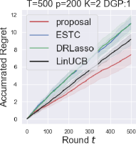
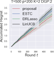
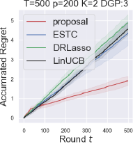
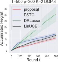
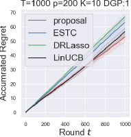
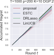
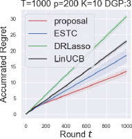
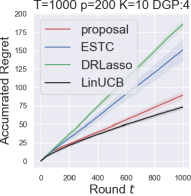
We consider two setups: and . For each setup, we consider a covariance matrix where and a base covariance for each , which represents a heterogeneous covariance among the arms. The base covariance follows the following configurations: DGP 1: , DGP 2: , DGP 3: , and DGP 4: and for . Note that the DGPs 1 and 3 correspond to Examples 2 and 1 in Proposition 1. DGP 3 is benign as well, while DGP 4 is not. We generate from a centered -dimensional Gaussian with covariance , from a standard normal distribution which yields non-sparse parameter vectors, and by the linear model (1) with the noise with variance . We compare proposal (AEtC, ) to ESTC (Hao et al., 2020), LinUCB (Li et al., 2010; Abbasi-Yadkori et al., 2011), and DR Lasso Bandit (Kim and Paik, 2019).
Figure 1 illustrates the accumulated regret in relation to the round . In the first three benign DGPs, the AEtC consistently outperforms the other methods. In DGP 2, the advantage of AEtC is insignificant because the regret of any method is already small. This is because in DGP 2, a model with exponentially decaying behavior, only a small fraction of eigenvalues are important. However, AEtC performs significantly better than its competitors in DGP 1 and DGP 3, where the eigenvalues have a heavy-tail distribution. In a non-benign example of DGP 4, the proposed method is still comparable to LinUCB, which demonstrates the utility of an interpolating estimator.
 |
 |
 |
 |
 |
 |
 |
 |
References
- Abbasi-Yadkori et al. [2011] Yasin Abbasi-Yadkori, Dávid Pál, and Csaba Szepesvári. Improved algorithms for linear stochastic bandits. Advances in neural information processing systems, 24, 2011.
- Abe and Long [1999] Naoki Abe and Philip M. Long. Associative reinforcement learning using linear probabilistic concepts. In Proceedings of the Sixteenth International Conference on Machine Learning, ICML ’99, page 3â11, San Francisco, CA, USA, 1999. Morgan Kaufmann Publishers Inc. ISBN 1558606122.
- Agarwal et al. [2012] Deepak K. Agarwal, Bee-Chung Chen, Pradheep Elango, and Xuanhui Wang. Personalized click shaping through lagrangian duality for online recommendation. In SIGIR ’12, 2012.
- Auer et al. [2002] Peter Auer, Nicolò Cesa-Bianchi, and Paul Fischer. Finite-time analysis of the multiarmed bandit problem. Mach. Learn., 47(2-3):235–256, 2002. doi: 10.1023/A:1013689704352.
- Bartlett et al. [2020] Peter L Bartlett, Philip M Long, Gábor Lugosi, and Alexander Tsigler. Benign overfitting in linear regression. Proceedings of the National Academy of Sciences, 117(48):30063–30070, 2020.
- Bastani and Bayati [2020] Hamsa Bastani and Mohsen Bayati. Online decision making with high-dimensional covariates. Oper. Res., 68(1):276–294, 2020.
- Bosq [2000] Denis Bosq. Linear processes in function spaces: theory and applications, volume 149. Springer Science & Business Media, 2000.
- Chakraborty and Murphy [2014] Bibhas Chakraborty and Susan A. Murphy. Dynamic treatment regimes. Annual Review of Statistics and Its Application, 1(1):447–464, 2014.
- Chu et al. [2011] Wei Chu, Lihong Li, Lev Reyzin, and Robert Schapire. Contextual bandits with linear payoff functions. In Geoffrey Gordon, David Dunson, and Miroslav DudÃk, editors, Proceedings of the Fourteenth International Conference on Artificial Intelligence and Statistics, volume 15 of Proceedings of Machine Learning Research, pages 208–214. PMLR, 11–13 Apr 2011.
- Hao et al. [2020] Botao Hao, Tor Lattimore, and Mengdi Wang. High-dimensional sparse linear bandits. Advances in Neural Information Processing Systems, 33:10753–10763, 2020.
- Hara and Maehara [2017] Satoshi Hara and Takanori Maehara. Enumerate lasso solutions for feature selection. In Proceedings of the AAAI Conference on Artificial Intelligence, volume 31, 2017.
- Jang et al. [2022] Kyoungseok Jang, Chicheng Zhang, and Kwang-Sung Jun. Popart: Efficient sparse regression and experimental design for optimal sparse linear bandits. In NeurIPS, 2022.
- Kim and Paik [2019] Gi-Soo Kim and Myunghee Cho Paik. Doubly-robust lasso bandit. Advances in Neural Information Processing Systems, 32, 2019.
- Koltchinskii and Lounici [2017] Vladimir Koltchinskii and Karim Lounici. Concentration inequalities and moment bounds for sample covariance operators. Bernoulli, 23(1):110–133, 2017.
- Lai and Robbins [1985] T.L Lai and Herbert Robbins. Asymptotically efficient adaptive allocation rules. Advances in Applied Mathematics, 6(1):4–22, 1985. ISSN 0196-8858.
- Li et al. [2010] Lihong Li, Wei Chu, John Langford, and Robert E. Schapire. A contextual-bandit approach to personalized news article recommendation. In Proceedings of the 19th International Conference on World Wide Web, WWW ’10, page 661â670, New York, NY, USA, 2010. Association for Computing Machinery. ISBN 9781605587998.
- Li et al. [2022] Wenjie Li, Adarsh Barik, and Jean Honorio. A simple unified framework for high dimensional bandit problems. In International Conference on Machine Learning, pages 12619–12655. PMLR, 2022.
- Miolane and Montanari [2021] Léo Miolane and Andrea Montanari. The distribution of the lasso: Uniform control over sparse balls and adaptive parameter tuning. The Annals of Statistics, 49(4):2313–2335, 2021.
- Nakakita and Imaizumi [2022] Shogo Nakakita and Masaaki Imaizumi. Benign overfitting in time series linear model with over-parameterization. arXiv preprint arXiv:2204.08369, 2022.
- Oh et al. [2021] Min-hwan Oh, Garud Iyengar, and Assaf Zeevi. Sparsity-agnostic lasso bandit. In International Conference on Machine Learning, pages 8271–8280. PMLR, 2021.
- Rendle [2010] Steffen Rendle. Factorization machines. In Geoffrey I. Webb, Bing Liu, Chengqi Zhang, Dimitrios Gunopulos, and Xindong Wu, editors, ICDM 2010, The 10th IEEE International Conference on Data Mining, Sydney, Australia, 14-17 December 2010, pages 995–1000. IEEE Computer Society, 2010.
- Robbins [1952] Herbert Robbins. Some aspects of the sequential design of experiments. Bulletin of the American Mathematical Society, 58(5):527 – 535, 1952.
- Tang et al. [2013] Liang Tang, Rómer Rosales, Ajit Singh, and Deepak Agarwal. Automatic ad format selection via contextual bandits. In Qi He, Arun Iyengar, Wolfgang Nejdl, Jian Pei, and Rajeev Rastogi, editors, 22nd ACM International Conference on Information and Knowledge Management, CIKM’13, pages 1587–1594. ACM, 2013.
- Tsigler and Bartlett [2020] Alexander Tsigler and Peter L Bartlett. Benign overfitting in ridge regression. arXiv preprint arXiv:2009.14286, 2020.
- Van De Geer and Bühlmann [2009] Sara A Van De Geer and Peter Bühlmann. On the conditions used to prove oracle results for the lasso. Electronic Journal of Statistics, 3:1360–1392, 2009.
- Vershynin [2018] Roman Vershynin. High-dimensional probability: An introduction with applications in data science, volume 47. Cambridge university press, 2018.
- Wang et al. [2018] Xue Wang, Mingcheng Wei, and Tao Yao. Minimax concave penalized multi-armed bandit model with high-dimensional covariates. In International Conference on Machine Learning, pages 5200–5208. PMLR, 2018.
- Wang et al. [2022] Yuyan Wang, Long Tao, and Xian Xing Zhang. Recommending for a multi-sided marketplace with heterogeneous contents. In Proceedings of the 16th ACM Conference on Recommender Systems, RecSys ’22, page 456â459. Association for Computing Machinery, 2022. ISBN 9781450392785.
Appendix A Limitations
The following characterizes the limitations. We consider addressing these are interesting directions for future work.
-
•
More adaptive algorithms, such as ones based on upper confidence bounds: This paper considers the class of the explore-then-commit methods. In many bandit problems, the upper confidence bound (UCB) method provides better empirical performance since it adaptively balances exploration and exploitation. Applying UCB to this problem is important future work. The key challenge here is that such an adaptive estimator involves a biased selection of the context vectors, which requires a more adaptive error bound for a high-dimensional linear model, such as the self-normalized bound [Abbasi-Yadkori et al., 2011].
-
•
Lower bound of the problem: While we showed the optimal choice of by deriving a matching bound, this does not exclude the possibility of a more adaptive bandit algorithm (e.g., UCB) that achieves a better rate of regret. Explicit construction of the lower bound requires two different models where the probability of an accurate (low-regret) estimate in one model implies a misestimation in the other model. To our knowledge, such a process for our non-sparse high-dimensional model is challenging because, unlike the sparse bandit model where only a small amount of parameters are active, in the non-sparse regime, we need to devise two models where very large () number of non-equal coefficients and need to bound the KL divergence between such a large multivariate Gaussians.
-
•
Temporal correlation: This paper assumes temporal indepenence (i.e., are independent between ). While such an assumption is popular, allowing the temporal correlation widens the application of the framework. For example, the click probability of online advertisements depends on the period of time. There are some recent results that are potentially applicable in non-sparse high-dimensional regime (e.g., Nakakita and Imaizumi [2022]).
-
•
Exponentially decaying models: Our proposed AEtC has the ability to handle various types of polynomially-decaying eigenvalues. Exploring the inclusion of exponentially-decaying eigenvalues, such as Example 4 in Theorem 31 of Bartlett et al. [2020], would be an intriguing avenue to explore.
Appendix B Proofs on Risk Bounds
We give proofs on the upper bound in Theorem 2. The bound is derived from the risk bound in Tsigler and Bartlett [2020] and adapted for our setting. A significant difference here is that the budget , which characterizes the covariance matrices , and the sample size used for estimation have different values.
We give some additional notation. For a vector and , let is a sub-vector. Similarly, is a sub-vector with the rest of the terms. For a covariance matrix with eigenvalues , and are diagonal matrices with the subset of eigenvalues. Similarly, for the data matrix , denotes a sub-matrix with the first columns of , and denotes a sub-matrix with the rest of the columns .
Proof of Theorem 2.
For each , we study the bound on the risk . Using the fact that with where is an i.i.d. copy of , we first decompose as
Using the decomposition, we decompose the total error as
Here, denotes a bias term of the risk, and denotes a variance term.
In the following, we develop a bound on each of the terms. Fix . By Corollary 6 in Tsigler and Bartlett [2020], we achieve the following bounds with some constant , which holds with the desired probability. Here, we set is the -th largest eigenvalue of for .
| (13) | |||
| (14) |
Note that only the number of samples appears explicitly in the boundary, while the budget affects it only implicitly through .
We study the bound for the bias part in (13). Here, we set using the coherent rank. By Hölder’s inequality, we obtain
which follows the definition of the effective rank . We also apply the properties of the ranks and obtain
where is a constant. The second last inequality follows . About the variance term in (14), we simply obtain by their definitions.
Finally, we set and obtain the statement. ∎
Appendix C Proofs for EtC
C.1 Concentration of the Maximum Value
Lemma 10.
Let be sub-Gaussian random variables with common parameter . Let be the maximum of them101010These random variables can be dependent each other.. Then, we have
| (15) |
Proof of Lemma 10.
For any , we have
| (16) | ||||
| (17) | ||||
| (18) |
and thus
and taking yields the result. ∎
C.2 High-probability Confidence Bound
Lemma 11.
There exists such that, for any , with probability at least , event
| (19) | ||||
| (20) |
holds. Moreover, under , we have
| (21) |
for each .
Note that, in EtC, we have uniform exploration over arms, and thus .
Proof of Lemma 11.
Theorem 2 implies that for some , with probability at least , holds. Moreover, the union bound of this over arms implies holds with probability .
Using the definition of the optimal arm , we have
where and . Given at the end of round , for each is a sub-Gaussian random variable. Under the event , the variance of is bounded as
| (22) |
By using this and Lemma 10 on the maximum of sub-Gaussian random variables, we have,
| (23) | ||||
| (24) |
∎
C.3 Proof of Theorem 4
C.4 Proof of Theorem 5
This section provides the regret lower bound of EtC.
Proof of Theorem 5.
We consider a model with . Let . We explicitly construct as follows: First, are identical and benign, and denote -th eigenvalue as . The coefficient , , and . With these , the only non-zero coefficients are , and thus the best arm is defined in terms of , which are the first components of , respectively.
Let be regret during the exploration and exploitation phases, respectively.
Regret during the exploration phase:
We first bound the regret during the exploration phase where we draw an arm uniformly randomly. In the following, we show that the regret per round is .
Since is a zero-mean (-dimensinal) Gaussian, its linear function such as are are zero-mean univariate Gaussians given .
Therefore,
is also a Gaussian, and its variance is . Therefore, . The regret in the rounds we draw arm is at least , which implies the regret-per-round is .
In summary, .
Regret during the exploitation phase:
We then bound the regret during the exploitation phase. Intuitively speaking, an algorithm misidentifies the better arm among and with probability and the regret per such a misidentification is .
Theorems 2 and Lemma 3 state that there exists a constant such that probability at least , for all we have
| (25) |
for some constants .
Without loss of generality, we assume to be sufficiently large such that because if then the size of the error bound is at least polylogarithmic, which results in regret of . In the following, we assume Eq. (25) is the case, and we show that the regret-per-round is . We define the events as follows:
| (26) | ||||
| (27) |
Event states that arm is positive and not very large, Event states that the algorithm draws considers the arm is the best and arm is the second best.
If is the case, then arm is chosen but suboptimal, and the regret is at least
| (28) |
where we used , , and . Therefore, showing
| (29) |
suffices to show that regret-per-round is . First, is a Gaussian with scale , which implies occurs with probability . Second, conditioned on , the sufficient condition for is
| (30) |
where
is an inner product that ignores the first component. Here, under Eq. (25), each of , , and , is a Gaussian random variables with its standard deviation . By this fact it is clear that . Therefore, . In summary, occurs with probability , and thus regret-per-round is by Eq. (28).
In summary, , and the expected regret is bounded as
| (31) | ||||
| (32) |
which completes the proof. ∎
Appendix D Proofs for AEtC
D.1 Proof of Lemma 6
We derive a high-probability bound of
| (33) | ||||
| (34) | ||||
| (by Lemma 12 with , transformation above follows with probability ) | (35) | |||
| (36) | ||||
| (by (Example 1) or (Example 2)) | (37) | |||
from which Lemma 6 follows.
Lemma 12.
Suppose that Assumption 1 holds. Assume that . Let the empirical covariance matrix with samples be
| (38) |
Then, for any , with probability at least , we have
for some constant .
Proof of Lemma 12.
We have
| (39) | ||||
| (40) | ||||
| (41) | ||||
| (42) |
and thus
| (43) |
Each diagonal element of is a sum of independent samples, and each sample is zero-mean sub-exponential random variable. Using Lemma 12 in Bartlett et al. [2020], with probability at least , we have
| (44) |
for some , which completes the proof. ∎
D.2 Proof of Lemma 7
Lemma 13.
(Lemma 4.2 in Bosq [2000]) For any two matrices with their eigenvalues and , we have
| (45) |
Lemma 14 (Corollary 2 in Koltchinskii and Lounici [2017]).
Suppose that are -valued i.i.d. random vectors whose mean is zero and covariance is . is an empirical covariance matrix. Then, there exists a constant and with probability we have
| (46) |
where
D.3 Proof of Lemma 8
This section adopts the same set of assumptions as Lemma 8.
Lemma 15.
Let be a constant that is independent of . Then, for any , with probability at least , we have
| (47) |
Proof of Lemma 15.
We assume Eq. (10) that holds with probability . We have,
| (48) | ||||
| (49) | ||||
| (50) |
where we have used in the last transformation. ∎
Lemma 16.
For and any , with probability at least , we have
Moreover, we have
for any .
Proof of Lemma 16.
We first show the first eigenvalues are negligible for : Namely,
| (51) |
Moreover, we have
| (52) | ||||
| (53) | ||||
| (54) | ||||
| (55) | ||||
| (56) | ||||
| (57) |
By definition,
| (58) | ||||
| (59) |
Eq. (57) states that , and by using the fact that (Example 1) or (Example 2), we have , which is equivalent to
| (60) |
∎
Lemma 17.
For any , with probability at least , we have