The correlations of stellar tidal disruption rates with properties of massive black holes and their host galaxies

Abstract

Stars can be either disrupted as tidal disruption events (TDEs) or swallowed as a whole by massive black holes (MBHs) at galactic centers when they approach sufficiently close to these MBHs. In this work, we investigate the correlations of such stellar consumption rates with both the MBH mass $M_{\rm BH}$ and the inner slope of the host galaxy mass density distribution $\alpha$. We introduce a simplified analytical power-law model with a power-law stellar mass density distribution surrounding MBHs and separate the contributions of two-body relaxation and stellar orbital precession for the stellar orbital angular momentum evolution in nonspherical galaxy potentials. The stellar consumption rates derived from this simplified model can be well consistent with the numerical results obtained with a more realistic treatment of stellar distributions and dynamics around MBHs, providing an efficient way to estimate TDE rates. The origin of the correlations of stellar consumption rates with $M_{\rm BH}$ and $\alpha$ are explained by the dependence of this analytical model on those MBH/host galaxy properties and by the separation of the stellar angular momentum evolution mechanisms. We propose that the strong positive correlation between the rates of stellar consumption due to two-body relaxation and $\alpha$ provides one interpretation for the overrepresentation of TDEs found in some rare E+A/poststarburst galaxies. We find high TDE rates for giant stars, up to those for solar-type stars. The understanding of the origin of the correlations of the stellar consumption rates will be necessary for obtaining the demographics of MBHs and their host galaxies via TDEs.

1 Introduction

Tidal disruption event (TDE) happens when a star travels too close to a massive black hole (MBH) so that the tidal force exerted on the star by the MBH surpasses the star’s self-gravity, causing the star to be ripped apart and disrupted, accompanied by luminous flares due to subsequent accretion of the stripped stellar material (e.g., Hills, 1975; Rees, 1988). TDEs may frequently occur at the centers of galaxies, as observations have shown the ubiquitous existence of MBHs (with mass ${\sim}10^{6}$–$10^{10}{M_{\odot}}$) at galactic nuclei (e.g., Ferrarese & Merritt 2000; Gebhardt et al. 2000; Tremaine et al. 2002; Kormendy & Ho 2013; Graham 2016). These TDEs provide rich electromagnetic signals, which help to study the relativistic effects, accretion physics, formation of radio jets and interior structure of torn stars, etc. (Komossa, 2015; Alexander, 2017; Gezari, 2021).

TDEs illuminate those dormant MBHs, and the event rates in individual galaxies depend on the MBH properties (e.g., Magorrian & Tremaine 1999, hereafter MT99; Wang & Merritt 2004; Ivanov et al. 2005; Kesden 2012; Fialkov & Loeb 2017). Therefore, they can serve as powerful probes of the MBH demographics, such as the MBH mass, spin, binarity, and the occupation fraction of MBHs in galaxies (Gezari, 2021). Depending on the event rate, the consumption of intruding stars may provide an important channel for the growth of MBHs in the centers of galaxies (Freitag & Benz, 2002; Yu, 2003; Brockamp et al., 2011; Alexander, 2017) and even has significant effects on the MBH spin evolution (Zhang et al., 2019), especially for those relatively less massive ones.

TDEs are first discovered as energetic transients in the soft X-ray band by archival searches of the ROSAT All-Sky Survey data (Bade et al., 1996; Grupe et al., 1999; Komossa & Greiner, 1999; Greiner et al., 2000) and later found via searches by multi-wavelength (e.g., UV, optical, X-ray, and gamma-ray) observations (Alexander, 2017; Gezari, 2021). Over the past decade, statistically significant samples of TDEs have begun to accumulate, largely owing to the rapid advancement of the optical time domain surveys, such as PTF (Law et al., 2009; Rau et al., 2009), ASAS-SN (Shappee et al., 2014), Pan-STARRS (Chambers et al., 2016), and ZTF (Bellm et al., 2019). For example, a recent census by Gezari (2021) listed $56$ TDE candidates, among which around two thirds are discovered by the wide-field optical time domain surveys. Based on different samples of TDE candidates, the TDE event rate is estimated to be ${\sim}10^{-5}$–$10^{-4}{\rm\,yr^{-1}}{\rm\,gal^{-1}}$ (e.g., Donley et al. 2002; Esquej et al. 2008; Maksym et al. 2010; Wang et al. 2012; van Velzen & Farrar 2014; Khabibullin & Sazonov 2014; Auchettl et al. 2018; van Velzen 2018).

Some recent studies on the TDE host galaxies reveal intriguingly that TDEs prefer those rare E+A/poststarburst galaxies (Arcavi et al., 2014; French et al., 2016, 2017; Law-Smith et al., 2017; Graur et al., 2018; Hammerstein et al., 2021). After removing the accountable selection effects (e.g., MBH mass, redshift completeness, strong active galactic nucleus presence, bulge colors and surface brightness), the remaining factor of the overrepresentation of TDEs in those rare subclass of galaxies is ${\sim}$25–48 (Law-Smith et al., 2017). The underlying mechanism(s) responsible for this preference is still unclear. Some proposed explanations include binary MBH formation due to a recent galaxy merger, stellar orbital perturbations induced by what has also caused the starburst in the past, a unique population of stars such as an evolved population of A giants which are susceptible for disruptions, and high central stellar density distributions or concentrations (e.g., see Alexander 2017; Law-Smith et al. 2017; French et al. 2020; Gezari 2021). To properly interpret these observations and thereby distinguish different dynamical mechanisms occurring in the galactic nuclei to produce TDEs, it is necessary to have a thorough understanding of these mechanisms, especially on the dependence of those theoretically predicted rates on the properties of the central MBHs and their host galaxies.

In a spherical stellar system composed of a central MBH and surrounding stars, the tidal radius for a given type of stars and the MBH event horizon determine the size of the loss cone in the phase space of the stellar energy and angular momentum, in the sense that a star at a given energy can be consumed (either tidally disrupted or swallowed as a whole) by the MBH when its angular momentum falls below a critical value. The rate of stellar consumptions is determined by the refilling rate of low-angular-momentum stars into the loss cone, since stars initially in the loss cone will be quickly consumed (e.g., within an orbital period). The two-body relaxation process of stars can set a lower limit for the refilling rate of low-angular-momentum stars into the loss cone. In realistic stellar systems, some other mechanisms may also work or even play a dominant role in refilling the loss cone, and therefore enhance the stellar consumption rates. Possible mechanisms include the resonant relaxation (Rauch & Tremaine, 1996; Hopman & Alexander, 2006), massive perturbers which may accelerate the two-body relaxation process (Perets et al., 2007), binary MBHs or recoiled MBHs (Ivanov et al., 2005; Chen et al., 2011; Stone & Loeb, 2011), as well as the stellar orbital precession within nonspherical galaxy gravitational potentials (MT99; Yu 2002; Vasiliev 2014).

In an earlier work (Chen et al. 2020b, hereafter CYL20), a statistical study is conducted on the cosmic distributions of stellar tidal disruptions by MBHs at galactic centers, due to the combined effects of two-body relaxation and orbital precession of stars in triaxial galaxy potentials; and the statistical results reveal the correlations of the stellar consumption rate with both the MBH mass $M_{\rm BH}$ and the inner slope of the galaxy surface brightness profile $\gamma$. A negative correlation between the stellar consumption rate (per galaxy) with the MBH mass (e.g., Wang & Merritt 2004; Stone & Metzger 2016) is found to exist only for $M_{\rm BH}\lesssim 10^{7}{M_{\odot}}$, and the correlation becomes positive for $M_{\rm BH}\gtrsim 10^{7}{M_{\odot}}$. At a given MBH mass $M_{\rm BH}$, the stellar consumption rate is higher in galaxies with larger $\gamma$ (steeper inner surface brightness profile) if $M_{\rm BH}\lesssim 10^{7}{M_{\odot}}$, but insensitive to $\gamma$ for MBHs with larger masses. In triaxial galaxy potentials, the phase space of the loss cone described for spherical galaxies can be replaced by the phase space of a general loss region to incorporate the stars that can precess onto low angular momentum orbits. The dichotomic trends of the stellar consumption rate at different MBH mass ranges can be explained by that the dominant fluxes of stellar consumption have different origins of the stellar low-angular-momentum orbits.

A further quantitative understanding of the origin of these correlations is of great importance as it provides the key to distinguish the dominant mechanism(s) of TDEs under different circumstances. Apart from that, the current and future TDE observations shed new light on the demographic studies of the MBH population, especially the mass function and the occupation fraction of MBHs at the low-mass end (e.g., Stone & Metzger 2016; Fialkov & Loeb 2017); the correlations of the stellar consumption with the MBH/galaxy properties cannot be ignored in a proper interpretation of the observational results, and should be accompanied with a quantitative understanding of the origin. To understand the origin of these correlations, we employ an analytical model considering power-law stellar distribution under the Keplerian potential of the central MBH. We first verify that this simplified model provides a fairly good approximation when evaluating the event rate of stellar consumption due to the two mechanisms, i.e., two-body relaxation and stellar orbital precession in nonspherical potentials. Then we identify the dominant factor(s) responsible for the slope and the scatter of each correlation.

The paper is organized as follows. In Section 2, we first briefly describe the galaxy sample used in this study. Then with the sample galaxies, we show the correlations of the stellar consumption rates with the MBH mass and the galaxy inner stellar distribution, as obtained in CYL20. In Section 3, we construct the analytical model and obtain the approximated expression for the stellar consumption rate due to either mechanism and inspect the contribution from different terms in the approximated expressions to these correlations. In Section 4, we explore the possibility of using such correlations to explain the observed overrepresentation of TDEs in those rare E+A/poststarburst galaxies. Based on the quantitative correlations constructed from the analytical model, we also generalize the discussion from the consumption rates of solar-type stars to those of other different types of stars.

2 Galaxy sample and rate correlations

2.1 Galaxy sample

In this study, we adopt the two observational samples of early-type galaxies given by Lauer et al. (2007) and Krajnović et al. (2013) to investigate the correlation between the stellar consumption rate by the central MBH and either the MBH mass or the host galaxy inner stellar distribution. For both samples, high-spatial-resolution observations of the galaxy surface brightness by $HST$ are available, which are crucial for TDE studies since stars from the inner region of the host galaxy (e.g., inside the influential radius of the central MBH) contribute significantly to the stellar consumption (MT99). Note that these two galaxy samples have also been adopted by CYL20 to study the cosmic distributions of the stellar tidal disruptions and by Chen et al. (2020a) to study the properties of the cosmic population of binary MBHs as well as their gravitational wave emissions.

For those early-type galaxies, their surface brightness profiles $I(R)$ can be well described by the Nuker law (Lauer et al., 1995). The best-fitting Nuker-law parameters for the sample galaxies can be found in each source paper. When calculating the stellar disruption/consumption rate, the mass-to-light ratio $M/L$ of the galaxy is also required, since $M/L$ and the surface brightness profile together determine the mass density distribution of the galaxy if it is spherically distributed. For galaxies in Lauer et al. (2007), we obtain their $M/L$ following Section 2.1 of Stone & Metzger (2016), i.e., their Equations (4)-(5). For galaxies in Krajnović et al. (2013), we note that their $r$-band $M/L$ can be found in Cappellari et al. (2013), but their Nuker-law parameters were fitted using the $V$-band observations. In this study, we assume that the $V$-band $M/L$ for these galaxies are the same as their $r$-band values. We estimate the MBH masses $M_{\rm BH}$ for the sample galaxies based on empirical scaling relations. For galaxies in Lauer et al. (2007), we follow Section 2.1 of Stone & Metzger (2016), i.e., adopting the $M_{\rm BH}$–$\sigma_{\rm e}$ relation from McConnell & Ma (2013) when $\sigma_{\rm e}$ is available in Lauer et al. (2007), while adopting the $M_{\rm BH}$–$L_{V}$ relation from McConnell & Ma (2013) otherwise. For galaxies in Krajnović et al. (2013), we adopt the $M_{\rm BH}$–$\sigma_{\rm e}$ relation from McConnell & Ma (2013), with $\sigma_{\rm e}$ taken from Cappellari et al. (2013). When studying the stellar consumption due to loss-region draining, we assume that each sample galaxy has a triaxial shape characterized by $p_{\rho}=0.9$ and $q_{\rho}=0.8$, where $p_{\rho}$ and $q_{\rho}$ represent the medium-to-major and minor-to-major axis ratios of the galaxy mass density distribution.

2.2 Stellar consumption rate correlations

In a spherical stellar system, the rate of stellar consumption by the central MBH due to two-body relaxation can be evaluated by solving the Fokker-Planck equation and the solution can be found in MT99 (see also Lightman & Shapiro 1977; Cohn & Kulsrud 1978), i.e.,

$${F^{\rm lc}}(\mathcal{E})d\mathcal{E}=\frac{4\pi^{2}\bar{f}(\mathcal{E})P(\mathcal{E})\bar{\mu}(\mathcal{E})J_{\rm c}^{2}(\mathcal{E})d\mathcal{E}}{\ln R_{0}^{-1}(\mathcal{E})}.$$ (1)

Here $\bar{f}(\mathcal{E})$ is the “isotropized” distribution function (see Eq. 21 of MT99), $P(\mathcal{E})\equiv P(\mathcal{E},J^{2}=0)$ is the orbital period of a test particle with “specific binding energy” $\mathcal{E}$ (hereafter abbreviated as energy) and zero “specific angular momentum” $J$ (hereafter abbreviated as angular momentum), $\bar{\mu}(\mathcal{E})$ is the orbital-averaged diffusion coefficient of the dimensionless angular momentum $R(\mathcal{E})\equiv J^{2}(\mathcal{E})/J_{\rm c}^{2}(\mathcal{E})$ in the limit $R\rightarrow 0$, with $J_{\rm c}(\mathcal{E})$ denoting the angular momentum of a star on a circular orbit with energy $\mathcal{E}$, $R_{0}(\mathcal{E})$ marks the value of $R(\mathcal{E})$ at which the distribution function falls to zero. $R_{0}(\mathcal{E})$ is given by

$$R_{0}(\mathcal{E})=R_{\rm lc}(\mathcal{E})\times\left\{\begin{split}&\exp(-q)&q\geq 1\\ &\exp(-0.186q-0.824\sqrt{q})&q<1\end{split},\right.$$ (2)

where $R_{\rm lc}(\mathcal{E})\equiv J^{2}_{\rm lc}(\mathcal{E})/J^{2}_{\rm c}(\mathcal{E})$ represents the relative size of the loss cone at energy $\mathcal{E}$ in the phase space, with $J_{\rm lc}$ denoting the loss-cone angular momentum and $q(\mathcal{E})\equiv P(\mathcal{E})\bar{\mu}(\mathcal{E})/R_{\rm lc}(\mathcal{E})$ representing the ratio of the change of $R(\mathcal{E})$ for radial orbits during an orbital period to $R_{\rm lc}(\mathcal{E})$ (MT99).

The stellar consumption rate due to loss-region draining in a nonspherical potential at a sufficiently long consumption time $T$ can be approximated by

$${F^{\rm drain}}(\mathcal{E})d\mathcal{E}=4\pi^{2}f(\mathcal{E})J_{\rm lc}^{2}(\mathcal{E})\exp\left[-\frac{T}{P(\mathcal{E})}\frac{J_{\rm lc}^{2}(\mathcal{E})}{J_{\rm lr}^{2}(\mathcal{E})}\right]d\mathcal{E},$$ (3)

where in triaxial galaxies $J_{\rm lr}(\mathcal{E})$ corresponds to the characteristic angular momentum at energy $\mathcal{E}$ below which stars can precess into the loss cone, and it is determined by the nonspherical shape of the host galaxy (see Eq. 9 in CYL20 and Eq. 52 in MT99). Due to the draining, stars initially inside the loss region are gradually depleted, and stars initially outside the loss region can be diffused into it due to two-body relaxation. As shown in CYL20, in triaxial galaxies, the loss-region refilling rate can be obtained by generalizing the analysis done for spherical systems, i.e., by replacing $J_{\rm lc}$ in Equations (1)–(2) with the angular momentum $J_{\rm lr}$ characterizing the size of the loss region. When the stars initially in the loss region are depleted significantly at $T\gg P(\mathcal{E}){J_{\rm lr}^{2}(\mathcal{E})}/{J_{\rm lc}^{2}(\mathcal{E})}$, the loss-region refilling rate due to two-body relaxation can be larger than the loss-region draining rate given by Equation (3) and thus dominate the stellar consumption rate.

When the loss-region refilling rate due to two-body relaxation dominates the stellar consumption rate, compared with the rate obtained through two-body relaxation in spherical systems, the correction of the stellar consumption rates for triaxial galaxies can be mainly due to the change of the logarithm term of $\ln R_{0}^{-1}(\mathcal{E})$ in Equations (1)–(2); and compared to the estimates for spherical systems, the average stellar consumption rates in triaxial galaxies are increased roughly by a similar factor of $f^{\rm tri}\sim$3–5 for low-mass MBHs (with masses ranging from $M_{\rm BH}\sim 10^{5}$–$10^{7}M_{\odot}$; see Figure 3 or 4 in CYL20). This rate increasing factor is almost independent of the MBH mass for low-mass MBHs (when $T\gtrsim 1$ Gyr; see Fig. 5 of CYL20). That is, the consumption rate–MBH mass correlation obtained by only considering two-body relaxation in spherical systems is similar to that by considering loss-region draining and refilling, except for a normalization difference by a factor of $f^{\rm tri}\sim 3-5$ (see Fig. 3 of CYL20). Thus, below for the purpose of this work on discussing the changing tendencies of the stellar consumption rates with properties of MBHs and host galaxies and for simplicity, we use Equations (1)–(2) obtained due to the two-body relaxation for spherical systems to analyze parts of the origin of the correlations.

The origin of the correlations of the stellar consumption rates with properties of MBHs and host galaxies can be analyzed through the functions of ${\mathscr{F}^{\rm lc}}=\int{F^{\rm lc}}(\mathcal{E})d\mathcal{E}$ or ${\mathscr{F}^{\rm drain}}=\int{F^{\rm drain}}(\mathcal{E})d\mathcal{E}$, where ${\mathscr{F}^{\rm lc}}$ is the total rate of stellar consumption due to two-body relaxation obtained by assuming that galaxies are spherical, and ${\mathscr{F}^{\rm drain}}$ is the total rate of stellar consumption due to the draining of the loss region obtained by assuming that galaxies are non-spherical. By taking into account that at some $\mathcal{E}$, ${F^{\rm drain}}(\mathcal{E})$ can become subdominant compared to the corresponding loss region refilling rate due to two-body relaxation, the stellar consumption rate (obtained by the integration over $\mathcal{E}$) in a triaxial galaxy, $\sim\int\max[f^{\rm tri}{F^{\rm lc}}(\mathcal{E}),{F^{\rm drain}}(\mathcal{E})]d\mathcal{E}$, is expected to be larger than $\max(f^{\rm tri}{\mathscr{F}^{\rm lc}},{\mathscr{F}^{\rm drain}})$, as well as being lower than the sum of $f^{\rm tri}{\mathscr{F}^{\rm lc}}+{\mathscr{F}^{\rm drain}}$. Thus the stellar consumption rate is expected to be $\sim{\mathscr{F}^{\rm drain}}$ if ${\mathscr{F}^{\rm drain}}\gg f^{\rm tri}{\mathscr{F}^{\rm lc}}$, and $\sim f^{\rm tri}{\mathscr{F}^{\rm lc}}$ if ${\mathscr{F}^{\rm drain}}\ll f^{\rm tri}{\mathscr{F}^{\rm lc}}$; As to be seen below (e.g., Figs. 1-2), both of those two cases cover a significantly large parameter space of host galaxy properties, so that the functions of ${\mathscr{F}^{\rm lc}}$ and ${\mathscr{F}^{\rm drain}}$ can be used to analyze the origin of the correlations of the stellar consumption rates. We estimate those stellar consumption rates of ${\mathscr{F}^{\rm lc}}$ and ${\mathscr{F}^{\rm drain}}$ for each sample galaxy according to Equations (1)–(3). We refer to CYL20 for some detailed procedures to calculate the relevant quantities in these equations.

Figure 1 shows the dependence of the stellar consumption rate due to two-body relaxation ${\mathscr{F}^{\rm lc}}$ on the MBH mass $M_{\rm BH}$ (left panel) and on the inner slope of the galaxy stellar number/mass density distribution $\alpha$ (right panel), respectively. The stellar consumption rate of each galaxy is evaluated based on Equation (1). As seen from this figure, ${\mathscr{F}^{\rm lc}}$ has a negative correlation with $M_{\rm BH}$, and a positive one with $\alpha$. We conduct linear fittings to the $\log{\mathscr{F}^{\rm lc}}-\log M_{\rm BH}$ relation (left panel) and the $\log{\mathscr{F}^{\rm lc}}-\alpha$ relation (right panel), respectively. The best-fitting relations are shown by the red dashed line in each panel, with the corresponding slope and intercept labeled in the panel. Similarly, in Figure 2, we show the dependence of the stellar consumption rate due to loss-region draining in nonspherical potentials ${\mathscr{F}^{\rm drain}}$ on the mass of the central MBH $M_{\rm BH}$ and on the inner slope of the galaxy stellar number/mass density distribution $\alpha$, where we set $T=10{\rm\,Gyr}$. In contrast to the case of two-body relaxation, ${\mathscr{F}^{\rm drain}}$ has a positive correlation with $M_{\rm BH}$ and a mildly negative correlation with $\alpha$. The best-fitting relations are also shown by the red dashed lines in both panels.

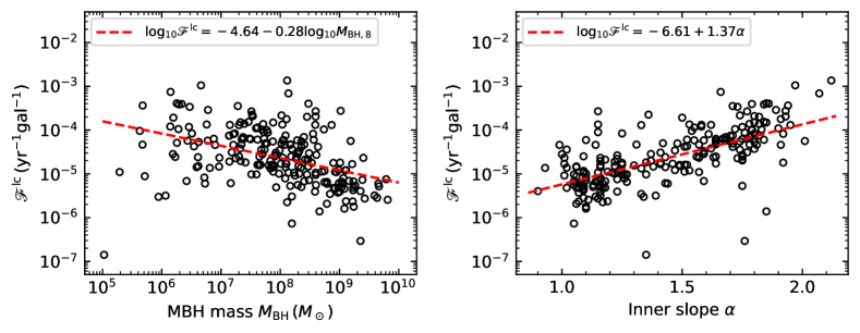
Figure 1: Dependence of the stellar consumption rate by the central MBH due to two-body relaxation ${\mathscr{F}^{\rm lc}}$ on the mass of the central MBH $M_{\rm BH}$ (left panel) and on the inner slope of the galaxy stellar number/mass density distribution $\alpha$ (right panel). Each open circle represents a galaxy in the sample. The red dashed lines in the left and the right panels represent the best fits to the correlation between ${\mathscr{F}^{\rm lc}}$ and $M_{\rm BH}$ and the correlation between ${\mathscr{F}^{\rm lc}}$ and $\alpha$, respectively. The best fit form is obtained by using the linear least square regression algorithm and is also labeled in each panel. This figure shows the slopes and scatters of both the correlation between ${\mathscr{F}^{\rm lc}}$ and $M_{\rm BH}$ and that between ${\mathscr{F}^{\rm lc}}$ and $\alpha$.

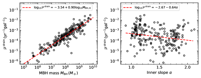
Figure 2: Legends are the same as those for Fig. 1, except that the stellar consumption is due to the draining of the loss region in nonspherical potentials. This figure shows the positive correlation between ${\mathscr{F}^{\rm drain}}$ and $M_{\rm BH}$, and the mildly negative correlation between ${\mathscr{F}^{\rm drain}}$ and $\alpha$.

As seen from Figures 1 and 2, we have ${\mathscr{F}^{\rm lc}}\gtrsim{\mathscr{F}^{\rm drain}}$ at $M_{\rm BH}\lesssim 10^{7}{M_{\odot}}$ and ${\mathscr{F}^{\rm lc}}\lesssim{\mathscr{F}^{\rm drain}}$ at $M_{\rm BH}\gtrsim 10^{7}{M_{\odot}}$. Correspondingly, we apply the correlations of ${\mathscr{F}^{\rm lc}}$ and ${\mathscr{F}^{\rm drain}}$ to interpret the correlation tendencies of the stellar consumption rates in those low-mass and high-mass ranges of MBHs, respectively.

Note that the fits shown in Figures 1 and 2 cover the whole MBH mass range, as it is a clear way to show the effects of the same mechanism through a large mass range. If the fit is limited to only a small mass range of $M_{\rm BH}\lesssim 10^{7}{M_{\odot}}$, specifically the correlation between ${\mathscr{F}^{\rm lc}}$ and $M_{\rm BH}$ could appear quite mild or may not be negative due to the small mass range and large rate scatters. In general, the other correlation tendencies are found not to be affected significantly even if limiting the fit mass range to either $M_{\rm BH}\lesssim 10^{7}{M_{\odot}}$ or $M_{\rm BH}\gtrsim 10^{7}{M_{\odot}}$. In this work, for connecting the stellar consumption rates with the underlying mechanisms and for simplicity, we use the fit results of the whole mass range below.

3 The power-law stellar distribution model

Table 1: Best-fit parameters and their $1\sigma$ uncertainties for the different correlations shown in Figures 1–2, 4, and 6.

	$\log_{10}Y=b_{M}+k_{M}\log_{10}M_{\rm BH,8}$			$\log_{10}Y=b_{\alpha}+k_{\alpha}\alpha$
$Y$	$b_{M}$	$k_{M}$		$b_{\alpha}$	$k_{\alpha}$
F^lc	-4.64(0.04)	-0.28(0.04)		-6.61(0.18)	1.37(0.12)
σ_h,200^3 M_BH,8^-1	-0.40(0.04)	-0.47(0.04)		-2.35(0.20)	1.37(0.13)
ζ(α)	-0.11(0.01)	-0.06(0.01)		-1.02(0.01)	0.63(0.00)
ϕ(ω)	-0.72(0.02)	0.26(0.02)		0.57(0.11)	-0.90(0.07)
F^drain	-3.54(0.03)	0.90(0.03)		-2.67(0.31)	-0.64(0.21)
χ(α)	0.26(0.01)	0.16(0.01)		1.18(0.04)	-0.64(0.03)
κ(M_BH,σ_h)	-0.37(0.04)	0.69(0.04)		-0.71(0.29)	0.20(0.19)
(R_lr,T/0.1)^25α-15	-0.18(0.01)	0.01(0.01)		0.12(0.02)	-0.21(0.02)

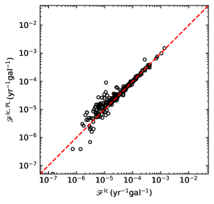
Figure 3: Comparisons of the calculated stellar consumption rates due to the two-body relaxation and those obtained approximately by adopting the simple power-law model described in Section 3, where the galaxies are assumed to be spherical. This figure verifies that the simple power-law model is effective in estimating the stellar consumption rates by the central MBHs due to the two-body relaxation, and therefore can be used to inspect the correlations of the stellar consumption rate with both the MBH mass and the inner stellar distribution of the galaxy.

The explanation to the correlations shown in Figures 1 and 2 obtained by using Equations (1)-(3) is not explicit, since many of the terms in these equations are calculated numerically for individual galaxies. In the following subsections, we employ a power-law model to obtain approximate expressions for the stellar consumption rates due to both the mechanisms. By saying “power-law model” we mean that the stellar number/mass density distribution of the galaxy can be described by a single power law and only the Keplerian potential of the central MBH is considered. We investigate the relative contributions of different terms in this simplified model to the stellar consumption rate and thus figure out the dominant factors that lead to these two correlations. As a counterpart, we define the “full model” as the one evaluating the stellar consumption rates through Equations (1)–(3). Below, we describe the details of the power-law model.

In the simplified model, we assume that the distribution of stars around the central MBH follows a single power law, i.e., $n_{\ast}(r)\propto r^{-\alpha}$ where $n_{\ast}(r)$ is the spatial number density of stars at radius $r$ and $\alpha$ is the power-law index. We define the influential radius of the MBH $r_{\rm h}$ to be the radius within which the enclosed stellar mass equals the MBH mass, i.e., $M_{\rm h}\equiv M_{\ast}(r\leq r_{\rm h})=M_{\rm BH}$. We make the power-law assumption based on the finding that stellar diffusion in the energy space gradually drives the distribution of stars in a system containing a central MBH towards a power-law cusp (Bahcall & Wolf, 1976). In practice, we adopt the Nuker law (Lauer et al., 1995) as a generic description of the surface brightness profiles of the galaxies. The break radii of realistic galaxies $R_{\rm b}$ are typically much larger than the influential radii of the MBHs $r_{\rm h}$, ensuring that the power-law density distribution a fairly good approximation for stars inside $r_{\rm h}$. Therefore, the spatial number density of stars surrounding the MBH could be formulated as

$$n_{\ast}(r)=\frac{(3-\alpha)N_{\rm h}}{4\pi r_{\rm h}^{3}}\left({\frac{r}{r_{\rm h}}}\right)^{-\alpha},$$ (4)

where $N_{\rm h}$ is the total number of stars enclosed in $r_{\rm h}$. The total number of stars enclosed in any given radius $r$ is $N_{\ast}(\leq r)=N_{\rm h}(r/r_{\rm h})^{3-\alpha}$. If we assume identical mass of stars, we also have $M_{\ast}(\leq r)=M_{\rm h}(r/r_{\rm h})^{3-\alpha}$, with $M_{\ast}(\leq r)$ being the total stellar mass enclosed in radius $r$. Throughout this paper, we make the approximation that $\alpha=\gamma+1$, where $\gamma$ is the inner slope of the Nuker-law surface brightness profile. It turns out to be a good approximation for sample galaxies with $\gamma\gtrsim 0.2$. For galaxies with $\gamma\lesssim 0.2$, the approximation tends to overestimate the inner slope of the host galaxy stellar number/mass density profile. However, the main conclusions obtained in this paper do not change by a small number of such galaxies in the sample.

In the power-law model, we ignore the self-gravity of the stellar system and assume that the potential is mainly contributed by the central MBH. We make this assumption based on the fact that the loss-cone consumption rate due to either mechanism peaks around the influential radius of the central MBH if we convert energy to radius based on the radial energy profile for stars in circular orbits, i.e., $\mathcal{E}(r)$. For example, for most of the sample galaxies, $\mathcal{E}{F^{\rm lc}}(\mathcal{E})$ peaks around $r_{\rm h}$ within a factor of $2$, while $\mathcal{E}{F^{\rm drain}}(\mathcal{E})$ peaks around $r_{\rm h}$ within a factor of $3$ when the consumption time is fixed to $T=10{\rm\,Gyr}$. Adopting a different $T$ does not significantly affect our results. Under the Keplerian potential of the central MBH, we evaluate the ergodic distribution function based on the Eddington’s formula. The resulting differential energy distribution of stars $N(\mathcal{E})d\mathcal{E}$ (i.e., the number of stars in the stellar system with energy in the range of $\mathcal{E}\rightarrow\mathcal{E}+d\mathcal{E}$) is expressed by

$$N(\mathcal{E})d\mathcal{E}=\xi(\alpha)N_{\rm h}\left(\frac{\mathcal{E}}{\mathcal{E}_{\rm h}}\right)^{\alpha-3}d\ln\mathcal{E},$$ (5)

where

$$\xi(\alpha)=\frac{\sqrt{\pi}}{8}(3-\alpha)2^{3-\alpha}\frac{\Gamma(\alpha+1)}{\Gamma(\alpha-\frac{1}{2})},$$ (6)

and $\mathcal{E}_{\rm h}\equiv\sigma_{\rm h}^{2}/2$ where $\sigma_{\rm h}^{2}\equiv GM_{\rm BH}/r_{\rm h}$.

3.1 Two-body relaxation mechanism

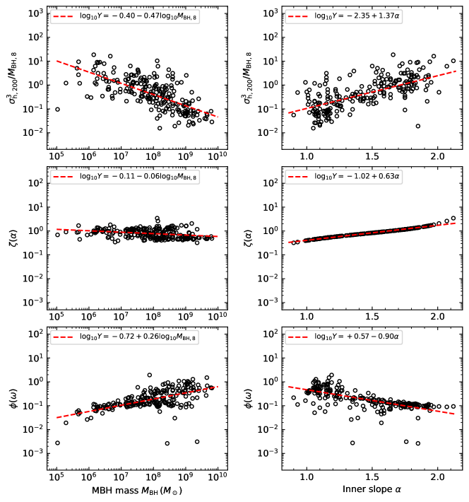
Figure 4: Dependence of the terms $\sigma^{3}M_{\rm BH}^{-1}$, $\zeta(\alpha)$, and $\phi(\omega)$ in the approximated stellar consumption rate due to the two-body relaxation in the power-law model ${\mathscr{F}^{\rm lc,PL}}$ (Eq. 10) on the MBH mass $M_{\rm BH}$ (left panels) and the inner slope of the host galaxy mass density distribution $\alpha$ (right panels). From top to bottom, the three inspected terms are ${\sigma_{\rm h}^{3}M_{\rm BH}^{-1}}$, $\zeta(\alpha)$ (Eq. 11), and $\phi(\omega)$ (Eq. 12), respectively. In the top two panels, $\sigma_{\rm h,200}$ and $M_{\rm BH,8}$ are $\sigma_{\rm h}$ and $M_{\rm BH}$ in unit of $200{\rm\,km\,s^{-1}}$ and $10^{8}{M_{\odot}}$, respectively. The best-fit is shown by the red dashed line in each panel, and the best fit form is also marked there with $Y$ representing the quantity of $\sigma_{\rm h,200}^{3}M_{\rm BH}^{-1}$, $\zeta(\alpha)$, and $\phi(\omega)$ in the top, middle, and bottom panels, respectively. Note that for the convenience of direct comparisons of the scatters with Fig. 1, all the panels here share the same decades along the $y$-axis with the panels in Fig. 1. This figure aims to reveal the dominant contributors to the slopes and scatters of both the correlation between ${\mathscr{F}^{\rm lc}}$ and $M_{\rm BH}$ and that between ${\mathscr{F}^{\rm lc}}$ and $\alpha$. See Section 3.1 for more details.

We first consider the stellar consumption due to the two-body relaxation by assuming the galaxy gravitational potential are spherical. When the Keplerian potential of the central MBH dominates, we have $P(\mathcal{E},J^{2})\simeq P(\mathcal{E})\simeq 2\pi GM_{\rm BH}/(2\mathcal{E})^{3/2}$; and the differential energy distribution can be expressed as $N(\mathcal{E})\simeq 4\pi^{2}f(\mathcal{E})P(\mathcal{E})J_{\rm c}^{2}(\mathcal{E})$ (i.e., see Eq. 5 of MT99). In this case, Equation (1) can be approximated as

$${F^{\rm lc}}(\mathcal{E})d\mathcal{E}\simeq\frac{N(\mathcal{E})\bar{\mu}(\mathcal{E})d\mathcal{E}}{\ln R_{0}^{-1}(\mathcal{E})}\simeq\frac{N(\mathcal{E})}{t_{\rm r}(\mathcal{E})}\frac{d\mathcal{E}}{\ln R_{0}^{-1}(\mathcal{E})},$$ (7)

where in the latter expression we have used the inverse of the relaxation timescale $1/t_{\rm r}(\mathcal{E})$ to approximate the orbital-averaged diffusion coefficient of the angular momentum, $\bar{\mu}(\mathcal{E})$. The relaxation timescale $t_{\rm r}(\mathcal{E})$ can be expressed as (see Bar-Or et al. 2013 and Eq. 1 of Alexander 2017)

$$t_{\rm r}(\mathcal{E})\simeq\eta\frac{Q^{2}P_{\rm c}(\mathcal{E})}{N_{\ast}(\leq r)\ln Q}\simeq\frac{2\pi\eta GM_{\rm BH}Q^{2}}{N_{\rm h}\sigma_{\rm h}^{3}\ln Q}\left(\frac{\mathcal{E}}{\mathcal{E}_{\rm h}}\right)^{3/2-\alpha},$$ (8)

where $\eta\simeq 1/8$, $Q\equiv M_{\rm BH}/\langle m_{\star}\rangle\simeq N_{\rm h}$ with $\langle m_{\star}\rangle$ representing the mean mass of stars, and $P_{\rm c}(\mathcal{E})$ is the orbital period of a circular orbit at energy $\mathcal{E}$. To get the rightmost expression in Equation (8), we assume the dominance of the Keplerian potential of the central MBH and use $r/r_{\rm h}\simeq(\mathcal{E}/\mathcal{E}_{\rm h})^{-1}$. Substituting Equations (5) and (8) into Equation (7), we have

$$\mathcal{E}{F^{\rm lc}}(\mathcal{E})\simeq\frac{\xi(\alpha)\sigma_{\rm h}^{3}\ln Q}{2\pi\eta GM_{\rm BH}\ln R_{0}^{-1}(\mathcal{E})}\left(\frac{\mathcal{E}}{\mathcal{E}_{\rm h}}\right)^{2\alpha-9/2}.$$ (9)

If we omit the variance of $\ln R_{0}^{-1}(\mathcal{E})$, which is a mildly decreasing function of $\mathcal{E}$ in the range $\mathcal{E}\gtrsim\mathcal{E}_{\rm h}$, then $\mathcal{E}{F^{\rm lc}}(\mathcal{E})$ is a decreasing function of $\mathcal{E}$ as long as $\alpha<9/4$, as seen from Equation (9). If the inner stellar distribution is core-like, i.e., $\alpha$ is small, $\mathcal{E}{F^{\rm lc}}(\mathcal{E})$ decreases relatively sharply with increasing $\mathcal{E}$, whereas if the inner stellar distribution is cusp-like with large $\alpha$, $\mathcal{E}{F^{\rm lc}}(\mathcal{E})$ decreases relatively mildly with increasing $\mathcal{E}$.

In real galaxies, $\mathcal{E}{F^{\rm lc}}(\mathcal{E})$ peaks at $\mathcal{E}_{\rm peak}\equiv\omega\mathcal{E}_{\rm h}$ where $\omega\simeq 1$. For $\mathcal{E}<\mathcal{E}_{\rm peak}$, the self-gravity from the stellar system cannot be neglected and Equation (9) does not work any more. As a matter of fact, $\mathcal{E}{F^{\rm lc}}(\mathcal{E})$ is an increasing function of $\mathcal{E}$ at $\mathcal{E}\leq\mathcal{E}_{\rm peak}$, instead of a decreasing function as described by Equation (9) for $\mathcal{E}>\mathcal{E}_{\rm peak}$. Therefore, the stellar consumption rate can be divided into two parts separated by $\mathcal{E}_{\rm peak}$. For the inner part with $\mathcal{E}\geq\mathcal{E}_{\rm peak}$, the rate can be approximated by integrating ${F^{\rm lc}}(\mathcal{E})$ over the range $\mathcal{E}\geq\mathcal{E}_{\rm peak}$ using Equation (9). For those real galaxies in our sample, we find that the fraction of the stellar consumption rate contributed by the inner part (i.e., with $\mathcal{E}\geq\mathcal{E}_{\rm peak}$) spans $0.1\sim 0.8$, and this fraction tends to be larger for a galaxy with a larger $\alpha$. Therefore, to compensate for the fraction of the rate contributed by those stars with $\mathcal{E}\leq\mathcal{E}_{\rm peak}$ which are omitted in the integration, we introduce a fudge factor ${f_{\omega}}$ by integrating ${F^{\rm lc}}(\mathcal{E})$ over the range $\mathcal{E}\geq{f_{\omega}}\mathcal{E}_{\rm peak}={f_{\omega}}\omega\mathcal{E}_{\rm h}$ using Equation (9). The resulting stellar consumption rate in the power-law model is given by

$${\mathscr{F}^{\rm lc,PL}} \simeq \int_{{f_{\omega}}\omega\mathcal{E}_{\rm h}}^{\infty}\mathcal{E}{F^{\rm lc}}(\mathcal{E})d\ln\mathcal{E}\simeq\frac{\zeta(\alpha)\sigma_{\rm h}^{3}({f_{\omega}}\omega)^{2\alpha-\frac{9}{2}}\ln Q}{2\pi\eta GM_{\rm BH}\ln R_{0}^{-1}(\omega\mathcal{E}_{\rm h})}$$ (10)

$$= \zeta(\alpha)\phi(\omega)\frac{\sigma_{\rm h}^{3}}{M_{\rm BH}}\frac{\ln Q}{2\pi G\eta},$$

where $\zeta(\alpha)$ and $\phi(\omega)$ are defined as

$$\zeta(\alpha)=\frac{2}{9-4\alpha}\cdot\xi(\alpha),$$ (11)

and

$$\phi(\omega)=\frac{({f_{\omega}}\omega)^{2\alpha-\frac{9}{2}}}{\ln R_{0}^{-1}(\omega\mathcal{E}_{\rm h})}.$$ (12)

We find that ${f_{\omega}}=1/2$ works well empirically. Therefore, we set ${f_{\omega}}=1/2$ in the following analysis if not stated specifically.

We compare the stellar consumption rates calculated from Equations (1)–(2) and those obtained approximately from the power-law model, as shown in Figure 3. Apparently, the rates estimated by using the simple power-law model are well consistent with those calculated from the full model (see Eqs. 1–3 and Chen et al. 2020b), which verifies the effectiveness of the simple power-law model in obtaining the correct rate and suggests the validity of using this simple model to inspect the correlations between ${\mathscr{F}^{\rm lc}}$ with both $M_{\rm BH}$ and $\alpha$. According to Equation (10), both the correlation between ${\mathscr{F}^{\rm lc}}$ and $M_{\rm BH}$ and that between ${\mathscr{F}^{\rm lc}}$ and $\alpha$ are controlled by three terms, i.e., ${\sigma_{\rm h}^{3}M_{\rm BH}^{-1}}$, $\zeta(\alpha)$, and $\phi(\omega)$. Figure 4 shows the dependence of the above three terms on the MBH mass $M_{\rm BH}$ (left panels) and the inner slope of the host galaxy mass density distribution $\alpha$ (right panels), separately. As seen from this figure, $\sigma_{\rm h}^{3}M_{\rm BH}^{-1}$ negatively correlates with $M_{\rm BH}$, $\phi(\omega)$ positively correlates with $M_{\rm BH}$, while the term $\zeta(\alpha)$ only weakly correlate with $M_{\rm BH}$; both $\sigma_{\rm h}^{3}M_{\rm BH}^{-1}$ and $\zeta(\alpha)$ positively correlate with $\alpha$, while $\phi(\omega)$ negatively correlates with $\alpha$, To describe the relative contribution of each term to the ${\mathscr{F}^{\rm lc}}-M_{\rm BH}$ relation and the ${\mathscr{F}^{\rm lc}}-\alpha$ relation quantitatively, we conduct a linear least square fitting to the data points shown in each panel of Figure 4. The best fit is shown by the red dashed line in each panel and its form is also labeled there. The best-fit parameters with their $1\sigma$ uncertainties are also listed in Table 1.

We identify the main factors that lead to the ${\mathscr{F}^{\rm lc}}-M_{\rm BH}$ relation and the ${\mathscr{F}^{\rm lc}}-\alpha$ relation quantitatively based on the fitting results (see Tab. 1 and legends in Figs. 1 and 4).

• For the ${\mathscr{F}^{\rm lc}}-M_{\rm BH}$ relation, the best fit gives a slope of $-0.28$ (left panel of Fig. 1). The best fits shown in the left panels of Figure 4 (from top to bottom) have slopes of $-0.47$, $-0.06$, and $0.26$, respectively. The sum of these three slopes is $-0.27$, which can approximately account for that found in the left panel of Figure 1. Among the three terms, ${\sigma_{\rm h}^{3}M_{\rm BH}^{-1}}$ dominates the total slope. The contribution from $\phi(\omega)$ can only cancel about half the amount of ${\sigma_{\rm h}^{3}M_{\rm BH}^{-1}}$, and $\zeta(\alpha)$ contributes the least to the total slope. Apart from the slope, the data points in the top left panel of Figure 4 have comparable scatters as those in the left panel of Figure 1, and are substantially larger than those in the middle left or the bottom left panel of Figure 4. Therefore, the intrinsic scatter of the ${\mathscr{F}^{\rm lc}}-M_{\rm BH}$ relation is also dominated by term ${\sigma_{\rm h}^{3}M_{\rm BH}^{-1}}$, i.e., by the intrinsic scatter of the correlation between ${\sigma_{\rm h}^{3}M_{\rm BH}^{-1}}$ and $M_{\rm BH}$, which is in turn determined by the scatter of the correlation between $\sigma_{\rm h}$ and $M_{\rm BH}$.

• For the ${\mathscr{F}^{\rm lc}}-\alpha$ relation, the best fit gives a slope of $1.37$ (right panel of Fig. 1). The best fits shown in the right panels of Figure 4 (from top to bottom) give slopes of $1.37$, $0.63$, and $-0.90$, respectively. The sum of these three slopes is $1.10$, which is close to that found for the ${\mathscr{F}^{\rm lc}}-\alpha$ relation (right panel of Fig. 1), again suggests that the correlation between ${\mathscr{F}^{\rm lc}}$ and $\alpha$ can be explained approximately by the combined effect of these three terms. Among the three terms, ${\sigma_{\rm h}^{3}M_{\rm BH}^{-1}}$ dominates the contribution to the total slope. While $\zeta(\alpha)$ and $\phi(\omega)$ contribute to the total slope in close amounts but different signs so as to be cancelled much. As seen also from the right panels of Figure 4, the scatters among the data points in the top panel dominate over those in the middle or bottom panels. Therefore, we can conclude that both the slope and the scatter of the correlation between ${\mathscr{F}^{\rm lc}}$ and $\alpha$ are dominated by the correlation between ${\sigma_{\rm h}^{3}M_{\rm BH}^{-1}}$ and $\alpha$.

3.2 Loss-region draining in nonspherical potentials

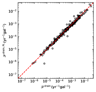
Figure 5: Legends are similar to that for Fig. 3, but the stellar consumption rates are due to the draining of loss region in nonspherical potentials.

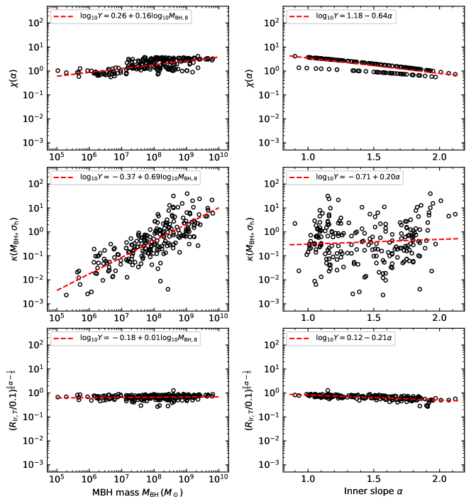
Figure 6: Dependence of the terms in the approximated stellar consumption rate due to draining of the loss region in nonspherical potentials in the power-law model ${\mathscr{F}^{\rm drain,PL}}$ (Eqs. 16 and 23) on the MBH mass $M_{\rm BH}$ (left panels) and the inner slope of the host galaxy mass density distribution $\alpha$ (right panels). From top to bottom, the three inspected terms are $\chi(\alpha)$ (Eq. 21), ${\kappa(M_{\rm BH},\sigma_{\rm h})}$ (Eq. 22), and ${(R_{{\rm lr},T}/0.1)^{\frac{2}{5}\alpha-\frac{1}{5}}}$ (Eq. 15), respectively. The best fit to the data is shown by the red dashed line in each panel, and the best fit form is also marked there with $Y$ representing $\chi(\alpha)$, ${\kappa(M_{\rm BH},\sigma_{\rm h})}$, and ${(R_{{\rm lr},T}/0.1)^{\frac{2}{5}\alpha-\frac{1}{5}}}$, respectively. For the convenience of direct comparisons of the scatters with Figure 2, all the panels here share the same decades along the $y$-axis with the panels in Figure 2. This figure aims to reveal the dominant contributors to the slopes and scatters of the correlations either between ${\mathscr{F}^{\rm drain}}$ and $M_{\rm BH}$ or between ${\mathscr{F}^{\rm drain}}$ and $\alpha$. See Section 3.2 for more details.

We now consider the correlation between ${\mathscr{F}^{\rm drain}}$ and $M_{\rm BH}$ or $\alpha$ in galaxies with nonspherical mass distributions. We define the loss-region draining timescale $\tau(\mathcal{E})\equiv P(\mathcal{E})J_{\rm lr}^{2}(\mathcal{E})/J_{\rm lc}^{2}(\mathcal{E})$, which characterizes how long the reservoir of loss-region stars at energy $\mathcal{E}$ can sustain the consumption by the central MBH. Similar as in the loss-cone case, we define the dimensionless loss-region angular momentum $R_{\rm lr}(\mathcal{E})\equiv J_{\rm lr}^{2}(\mathcal{E})/J_{\rm c}^{2}(\mathcal{E})$, which characterizes the relative size of the loss region at energy $\mathcal{E}$ in the phase space. In generic triaxial galaxies, $R_{\rm lr}(\mathcal{E})$ can reach the order of $\sim$0.1 at energies satisfying $\mathcal{E}\lesssim\mathcal{E}_{\rm h}$ and decreases with increasing $\mathcal{E}$ for $\mathcal{E}>\mathcal{E}_{\rm h}$. The draining timescale can be then expressed as $\tau(\mathcal{E})=P(\mathcal{E})R_{\rm lr}(\mathcal{E})/R_{\rm lc}(\mathcal{E})$. Therefore, the flux of stars being drained from the loss region into the loss cone to be consumed can be expressed as

$${F^{\rm drain}}(\mathcal{E})d\mathcal{E}\simeq\frac{N(\mathcal{E})R_{\rm lr}(\mathcal{E})d\mathcal{E}}{\tau(\mathcal{E})}\exp\left[-\frac{T}{\tau(\mathcal{E})}\right],$$ (13)

where we have again made the approximation $P(\mathcal{E},J^{2})\simeq P(\mathcal{E})\equiv P(\mathcal{E},J^{2}=0)$. Assuming the dominance of the Keplerian potential of the central MBH, we have $P(\mathcal{E})\simeq 2\pi GM_{\rm BH}/(2\mathcal{E})^{3/2}$ and $J_{\rm c}(\mathcal{E})\simeq GM_{\rm BH}/(2\mathcal{E})^{1/2}$. Define the consumption radius $r_{\rm consp}\equiv J^{2}_{\rm lc}/2GM_{\rm BH}$, then the loss-region draining timescale can be approximated as

$$\tau(\mathcal{E})\simeq\frac{\pi(GM_{\rm BH})^{2}R_{\rm lr}(\mathcal{E})}{4\sqrt{2}\mathcal{E}^{5/2}r_{\rm consp}}.$$ (14)

Since typically $\mathcal{E}{F^{\rm drain}}(\mathcal{E})$ is an increasing function of $\mathcal{E}$, the total stellar consumption rate at the draining time $T$ due to loss-region draining is dominated by the flux of stars at $\mathcal{E}\simeq\mathcal{E}_{T}$, with $\mathcal{E}_{T}$ satisfies $\tau(\mathcal{E}_{T})=T$, which gives

$$\mathcal{E}_{T}=\left[\frac{\pi(GM_{\rm BH})^{2}R_{\rm lr}{{}_{,T}}}{4\sqrt{2}Tr_{\rm consp}}\right]^{2/5},$$ (15)

where $R_{{\rm lr},T}=R_{\rm lr}(\mathcal{E}_{T})$. At energy $\mathcal{E}<\mathcal{E}_{T}$ where the loss region has not been exhausted yet, $\mathcal{E}{F^{\rm drain}}$ increases with $\mathcal{E}$ in a manner that $\mathcal{E}{F^{\rm drain}}\sim\mathcal{E}^{\alpha-1/2}$ in the power-law model. Therefore, the total stellar consumption rate due to the loss-region draining can be evaluated as

$${\mathscr{F}^{\rm drain,PL}} \simeq \frac{2}{2\alpha-1}f_{T}\mathcal{E}_{T}{F^{\rm drain}}(\mathcal{E}_{T})$$ (16)

$$= \frac{2\xi(\alpha)}{2\alpha-1}\frac{f_{T}N_{\rm h}R_{{\rm lr},T}}{T}\left(\frac{\mathcal{E}_{T}}{\mathcal{E}_{\rm h}}\right)^{\alpha-3},$$

where $\xi(\alpha)$ is given by Equation (6), $f_{T}$ is a fudge factor introduced to make the rates estimated by the power-law model consistent with those by the full model, and $f_{T}$ changes from $0.78$ at $T=0.1{\rm\,Gyr}$ to $0.56$ at $T=10{\rm\,Gyr}$. Since we analyze the rate correlations at $T=10{\rm\,Gyr}$, we adopt $f_{T}=0.56$ below.

The definition of the consumption radius $r_{\rm consp}$ naturally leads to a separatrix in the MBH mass $M_{\rm BH}$, below which $r_{\rm consp}=r_{\rm t}=(f_{\rm t}M_{\rm BH}/m_{\star})^{1/3}R_{\star}$, with $m_{\star}$ and $R_{\star}$ being the mass and radius of the star and $f_{\rm t}$ being a dimensionless factor, while above which $r_{\rm consp}=2r_{\rm swl}=8GM_{\rm BH}/c^{2}$ ($r_{\rm swl}\equiv 4GM_{\rm BH}/c^{2}$; see Eq. 1 in CYL20). For MBHs with masses being below the separatrix, setting $m_{\star}$ and $R_{\star}$ to be the solar mass and solar radius and $f_{\rm t}=1$, we have

$$\frac{\mathcal{E}_{T}}{\mathcal{E}_{\rm h}}=\left[\frac{\pi(GM_{\rm BH})^{2}R_{{\rm lr},T}}{Tr_{\rm consp}\sigma_{\rm h}^{5}}\right]^{\frac{2}{5}}$$

$$\simeq 1.24\left[\frac{M_{\rm BH}}{10^{8}{M_{\odot}}}\right]^{\frac{2}{3}}\left[\frac{\sigma_{\rm h}}{200{\rm\,km\,s^{-1}}}\right]^{-2}\left[\frac{R_{{\rm lr},T}}{0.1}\right]^{\frac{2}{5}}\left[\frac{T}{10{\rm\,Gyr}}\right]^{-\frac{2}{5}}.$$

(17)

Substituting Equation (17) into Equation (16), the stellar consumption rate due to the loss-region draining when the MBH mass is below the separatrix can be approximated in the power-law model as

$${\mathscr{F}^{\rm drain,PL}}\simeq 1.24^{\alpha-3}\frac{2\xi(\alpha)}{2\alpha-1}\times 10^{-3}f_{T}{\rm\,yr^{-1}}\left[\frac{M_{\rm BH}}{10^{8}{M_{\odot}}}\right]^{\frac{2\alpha-3}{3}}$$

$$\left[\frac{\sigma_{\rm h}}{200{\rm\,km\,s^{-1}}}\right]^{6-2\alpha}\left[\frac{R_{{\rm lr},T}}{0.1}\right]^{\frac{2\alpha-1}{5}}\left[\frac{10{\rm\,Gyr}}{T}\right]^{\frac{2\alpha-1}{5}}.$$

(18)

On the other hand, when the MBHs have masses being above the separatrix, we have

$$\frac{\mathcal{E}_{T}}{\mathcal{E}_{\rm h}}=\left[\frac{\pi(GM_{\rm BH})^{2}R_{{\rm lr},T}}{Tr_{\rm consp}\sigma_{\rm h}^{5}}\right]^{\frac{2}{5}}\simeq$$

$$0.735\left[\frac{M_{\rm BH}}{10^{8}{M_{\odot}}}\right]^{\frac{2}{5}}\left[\frac{\sigma_{\rm h}}{200{\rm\,km\,s^{-1}}}\right]^{-2}\left[\frac{R_{{\rm lr},T}}{0.1}\right]^{\frac{2}{5}}\left[\frac{T}{10{\rm\,Gyr}}\right]^{-\frac{2}{5}}.$$

(19)

Substituting Equation (19) into Equation (16), the corresponding stellar consumption rate due to the loss-region draining when the MBH mass is above the separatrix can be approximated in the power-law model as

$${\mathscr{F}^{\rm drain,PL}}\simeq 0.735^{\alpha-3}\frac{2\xi(\alpha)}{2\alpha-1}\times 10^{-3}f_{T}{\rm\,yr^{-1}}\left[\frac{M_{\rm BH}}{10^{8}{M_{\odot}}}\right]^{\frac{2\alpha-1}{5}}$$

$$\left[\frac{\sigma_{\rm h}}{200{\rm\,km\,s^{-1}}}\right]^{6-2\alpha}\left[\frac{R_{{\rm lr},T}}{0.1}\right]^{\frac{2\alpha-1}{5}}\left[\frac{10{\rm\,Gyr}}{T}\right]^{\frac{2\alpha-1}{5}}.$$

(20)

For the convenience of the following analysis, we define

$$\chi(\alpha)=\left\{\begin{split}1.24^{\alpha-3}\cdot\frac{2\xi(\alpha)}{2\alpha-1},\quad r_{\rm t}\geq 2r_{\rm swl},\\ 0.735^{\alpha-3}\cdot\frac{2\xi(\alpha)}{2\alpha-1},\quad r_{\rm t}<2r_{\rm swl}.\end{split}\right.$$ (21)

and

$$\kappa(M_{\rm BH},\sigma_{\rm h})=\left\{\begin{split}M_{\rm BH,8}^{\frac{2}{3}\alpha-1}\sigma_{\rm h,200}^{6-2\alpha},\quad r_{\rm t}\geq 2r_{\rm swl},\\ M_{\rm BH,8}^{\frac{2}{5}\alpha-\frac{1}{5}}\sigma_{\rm h,200}^{6-2\alpha},\quad r_{\rm t}<2r_{\rm swl}.\end{split}\right.$$ (22)

With these definitions, the stellar consumption rate due to the loss-region draining in the power-law model can be expressed as

$${\mathscr{F}^{\rm drain,PL}} \simeq 10^{-3}f_{T}{\rm\,yr^{-1}}\chi(\alpha)\kappa(M_{\rm BH},\sigma_{\rm h})\times$$ (23)

$$\left[\frac{R_{{\rm lr},T}}{0.1}\right]^{\frac{2\alpha-1}{5}}\left[\frac{10{\rm\,Gyr}}{T}\right]^{\frac{2\alpha-1}{5}}.$$

In the following, we fix the consumption time to $T=10{\rm\,Gyr}$.

Similarly as done for the case of the two-body relaxation, we compare the stellar consumption rates calculated from Equation (3) and those obtained approximately from the power-law model (Eq. 23) as shown in Figure 5. As seen from the figure, the rates evaluated based on these two approaches are generally consistent with each other which again verifies the effectiveness of the power-law model in estimating the stellar consumption rate due to the loss-region draining in nonspherical potentials.

According to Equation (23), both the correlation between ${\mathscr{F}^{\rm drain}}$ and $M_{\rm BH}$ and that between ${\mathscr{F}^{\rm drain}}$ and $\alpha$ are controlled by the terms of $\chi(\alpha)$, $\kappa(M_{\rm BH},\sigma_{\rm h})$, and $\left(\frac{R_{{\rm lr},T}}{0.1}\right)^{\frac{2\alpha-1}{5}}$, and Figure 6 shows the dependence of these three terms on $M_{\rm BH}$ (left panels) and $\alpha$ (right panels), separately. As done for those correlations shown in Figure 4, we also conduct linear least square fittings to the data points shown in each panel of Figure 6. The best fit is indicated by the red dashed line in each panel and the best fit form is also labeled there. The best-fit parameters with their $1\sigma$ uncertainties are also listed in Table 1.

We use the fitting results to identify the main factors that contribute to the correlation between ${\mathscr{F}^{\rm drain}}$ and $M_{\rm BH}$ and that between ${\mathscr{F}^{\rm drain}}$ and $\alpha$ (see Tab. 1 and legends in Figs. 2 and 6).

• As seen from the left panel of Figure 2, the ${\mathscr{F}^{\rm drain}}$–$M_{\rm BH}$ correlation has a slope of $0.90$. While according to the left panels of Figure 6, the correlations between those three inspected terms (in logarithm) and $\log M_{\rm BH}$ have slopes of $0.16$, $0.69$, and $0.01$, respectively. Overall, these three relations combined can well account for the correlation between ${\mathscr{F}^{\rm drain}}$ and $M_{\rm BH}$. Among the three terms, ${\kappa(M_{\rm BH},\sigma_{\rm h})}$ dominates the correlation, which scales as $\sim\sigma_{\rm h}^{3}$ and $\sim\sigma_{\rm h}^{3}M_{\rm BH}^{2/5}$ when $M_{\rm BH}$ is below and above the separatrix, respectively, if setting $\alpha=3/2$. In addition, the term $\chi(\alpha)$ contributes minorly to the correlation. By comparing the data points in the left panels of Figure 6 and the left panel of Figure 2, it is clearly revealed that the scatter of the correlation between ${\mathscr{F}^{\rm drain}}$ and $M_{\rm BH}$ is also dominated by ${\kappa(M_{\rm BH},\sigma_{\rm h})}$.

• As seen from the right panel of Figure 2, there exist considerable scatters among the data points. Given the scatters, the correlation between ${\mathscr{F}^{\rm drain}}$ and $\alpha$ appears to be mild. A negative slope ($-0.64$) is returned when the linear square regression is applied to the data points, suggesting a decrease of about a factor of $4$ from $\alpha=1$ to $\alpha=2$. From the right panels of Figure 6, the best-fit slopes of the three inspected terms (in logarithm) against $\alpha$ are $-0.64$, $0.20$, and $-0.21$, respectively. Again, these three relations combined together can well account for that correlation between ${\mathscr{F}^{\rm drain}}$ and $\alpha$. Among the three terms, $\chi(\alpha)$ dominates the correlation. The scatter of the correlation is largely contributed by the term of ${\kappa(M_{\rm BH},\sigma_{\rm h})}$.

4 Discussions

4.1 Overrepresentation of TDEs in E+A/poststarburst galaxies

Some recent studies towards TDE host galaxies suggest that TDEs prefer to happen in those rare E+A/poststarburst galaxies (Arcavi et al., 2014; French et al., 2016, 2017; Law-Smith et al., 2017; Graur et al., 2018; Hammerstein et al., 2021). The underlying (physical) explanations for the preference are still unclear, and there may be alternative characteristics to distinguish TDE host galaxies from normal ones (Law-Smith et al., 2017). Here we discuss whether the preference can be explained by the correlations between the stellar consumption rate and the inner slope of the galaxy stellar number/mass density distribution. Since TDE flares can only be observed when the MBH mass is below the Hills’ mass (Hills, 1975), in which regime the two-body relaxation mechanism dominates over the stellar orbital precession mechanism (CYL20), we focus on the correlation between ${\mathscr{F}^{\rm lc}}$ and $\alpha$.

To explore whether the overrepresentation can be explained by the high central stellar density of the galaxies, Law-Smith et al. (2017) identified a region in the Sersic index and MBH mass parameter space which contained ${\sim}2\%$ of their reference catalog galaxies but $\geq 60\%$ of those TDE host galaxies. This means that the averaged TDE rate in those high-Sersic-index galaxies should be higher than that in their low-Sersic-index counterparts by a factor of ${\sim}25-48$. From the right panel of Figure 1, the mean value of $\log{\mathscr{F}^{\rm lc}}$ increases by $1.37$ when $\alpha$ is increased from $1$ to $2$, or equivalently when $\gamma$ (the inner slope of the galaxy surface brightness profile) is increased from $0$ to $1$. As also seen from the panel, the intrinsic scatter of the correlation has no significant dependence on $\alpha$. Therefore, the averaged consumption rate $\langle{\mathscr{F}^{\rm lc}}\rangle$ is increased by a factor of ${\sim}24$ from $\alpha=1$ to $\alpha=2$, which is within a factor of $2$ of the analysis by Law-Smith et al. (2017). Given the limited number of TDEs in the observational analysis (i.e., 5–10 events), it suggests that the correlation between ${\mathscr{F}^{\rm lc}}$ and $\alpha$ may be responsible for the overrepresentation reported by recent studies towards TDE host galaxies.

The overrepresentation may also be contributed by draining of the loss-region stars in nonspherical potentials, as those poststarburst systems may also have a higher degree of asymmetry in their shapes as compared with generic galaxies. The presence of A type stars in the nuclear regions of those E+A/poststarburst galaxies indicates their relatively young ages and dynamical states (e.g., French et al. 2017; Law-Smith et al. 2017), and therefore a relatively full loss region and a larger draining rate. As the loss region draining rate ${\mathscr{F}^{\rm drain}}$ decreases with increasing time $T$, we can define the time $T_{\rm eq}$ at which the loss region draining rate ${\mathscr{F}^{\rm drain}}(T=T_{\rm eq})$ equals to the loss cone refilling rate $f^{\rm tri}{\mathscr{F}^{\rm lc}}$. We have ${\mathscr{F}^{\rm drain}}(T)\gtrsim f^{\rm tri}{\mathscr{F}^{\rm lc}}$ at $T\lesssim T_{\rm eq}$ and ${\mathscr{F}^{\rm drain}}(T)\lesssim f^{\rm tri}{\mathscr{F}^{\rm lc}}$ at $T\gtrsim T_{\rm eq}$. By using the scaling dependence of ${\mathscr{F}^{\rm drain,PL}}$ on time $T$ shown in Equation (23) (i.e., $\propto T^{(1-2\alpha)/5}$) and the scaling dependence of ${\mathscr{F}^{\rm drain}}$ and ${\mathscr{F}^{\rm lc}}$ on $M_{\rm BH}$ shown at $T=10{\rm\,Gyr}$ in Figures 1–2, we can obtain the time $T_{\rm eq}$ by

$$\left(\frac{2\alpha-1}{5}\right)\log\left(\frac{T_{\rm eq}}{10{\rm\,Gyr}}\right)\simeq 1.10-\log f^{\rm tri}+1.18\log M_{\rm bh,8}.$$ (24)

For example, we have $T_{\rm eq}\simeq 10{\rm\,Gyr}({f^{\rm tri}\over 3})^{-0.4}({M_{\rm BH}\over 3\times 10^{7}M_{\odot}})^{2.95}$ if $\alpha=3/2$ in Equation (24). Compared with the stellar consumption rate in a system with age $\sim 10{\rm\,Gyr}$, the enhancement of stellar consumption rate due to the draining of the loss-region stars in a young system with dynamical age $T$ can be estimated by a factor of ${{\mathscr{F}^{\rm drain}}(T)\over{\mathscr{F}^{\rm drain}}[\min(10{\rm\,Gyr},T_{\rm eq})]}\simeq[{\min(10{\rm\,Gyr},T_{\rm eq})\over T}]^{\frac{2\alpha-1}{5}}$. If assuming the age $T=0.1{\rm\,Gyr}$, and $f^{\rm tri}\simeq 3$ and $\alpha=3/2$ in Equation (24), the factor is $\sim 6$ for $M_{\rm BH}\gtrsim 3\times 10^{7}M_{\odot}$ (for which $T_{\rm eq}\gtrsim 10{\rm\,Gyr}$) and smaller for lower MBH masses (e.g. $\sim 2$ for $M_{\rm BH}=10^{7}M_{\odot}$). Those estimation obtained from the above analytical scaling fittings are consistent with those shown in Figure 5 of CYL20.

Overall, the TDE event rate in the E+A galaxies may be enhanced by a factor of several tens as compared with generic galaxies. Among them, the effect due to larger $\alpha$ or higher central densities of E+A galaxies dominates the rate enhancement, while draining of the loss-region stars in these dynamically young systems may also contribute a factor of a few, depending on the dynamical age of the system and the MBH mass. We expect that the above explaination to the overrepresentation of the TDEs due to the different contributions will be testable through a significant accumulation of TDE observations along with observations of their host galaxy properties.

4.2 Generalization for different types of stars

In the above analysis, we assume a single stellar population with solar mass and solar radius. In reality, however, the stellar system is composed of a spectrum of stars with different masses $m_{\ast}$ and radii $R_{\ast}$. For each species in the stellar system, the mass separatrix of MBHs that can tidally disrupt or directly swallow low-angular-momentum stars is determined by a comparison of $r_{\rm t}$ and $2r_{\rm swl}$, as mentioned in Section 3.2. Different types of stars have different $M_{\rm BH}$ separatrixes between TDEs and direct capture events, which depend on stellar mass and radius by a scaling factor of $(m_{\ast}/M_{\odot})^{-\frac{1}{2}}(R_{\ast}/R_{\odot})^{\frac{3}{2}}$. In this subsection, we discuss how the mass spectrum may affect the stellar consumption rate estimations and their correlation tendencies and how our above scaling analysis can imply for the rates of different types of stars.

We discuss the effects of the mass spectrum on the stellar consumption rate estimations and their correlation tendencies through their effects on ${\mathscr{F}^{\rm lc}}$ and ${\mathscr{F}^{\rm drain}}$ as follows.

• ${\mathscr{F}^{\rm lc}}$: The overall stellar consumption rate due to two-body relaxation, ${\mathscr{F}^{\rm lc}}$, is not affected significantly by the generalization of the single-mass stellar population assumption (MT99). As shown in Appendix A in MT99, if replacing the single-mass stellar population with an old stellar population (e.g., the Kroupa initial mass function between $0.08M_{\odot}$ and $1M_{\odot}$), ${\mathscr{F}^{\rm lc}}$ will increase by a factor of $\sim 1.66$, due to the combined effects of the increased stellar number density and the decreased stellar diffusion rate. The consumption rate of a given type of stars is then roughly proportional to its number fraction among all the stars, if the mass segregation effect is not significant. However, if the mass segregation effect is important, then the consumption rate of high-mass stars may be further enhanced and that of low-mass stars may be weakened.

  For each species in the stellar system, the consumption rate due to two-body relaxation varies with the changes of the number fraction of the species and the logarithmic terms $\ln Q$ and $\ln R_{0}^{-1}(\mathcal{E})$ in Equations (9)–(10). If we ignore the generally weak variations of the two logarithmic terms, the ${\mathscr{F}^{\rm lc}}$ rate correlation tendencies due to two-body relaxation apply effectively to disrupted or swallowed stars of different types, including giant stars (with $m_{\ast}{\sim}M_{\odot}$, $R_{\ast}{\sim}10$–$1000R_{\odot}$) and white dwarfs (with $m_{\ast}{\sim}M_{\odot}$, $R_{\ast}{\sim}0.01R_{\odot}$).

• ${\mathscr{F}^{\rm drain}}$: The stellar consumption rate due to loss-region draining, ${\mathscr{F}^{\rm drain}}$, is affected by relaxing the single-type stellar population assumption in the following three aspects. (a) ${\mathscr{F}^{\rm drain}}$ is proportional to the number density of stars (corresponding to the $N_{\rm h}$ term in Eq. 16). If the single stellar population with solar mass and radius considered above in Section 3.2 is replaced by an old population of stars (e.g., the Kroupa initial mass function between $0.08M_{\odot}$ and $1M_{\odot}$), the change of the total stellar number density will lead to an increase of ${\mathscr{F}^{\rm drain}}$ by a factor of $5.33$. The rate of each given species is proportional to the number fraction of the given species. (b) ${\mathscr{F}^{\rm drain}}$ can also depend on mass and radius of each type of stars via their different loss-cone size or the consumption radius $r_{\rm consp}$. According to Equations (15) and (16), we have ${\mathscr{F}^{\rm drain}}\propto{r_{\rm consp}}^{{-2\alpha+6}\over 5}$, which is $\propto(m_{\ast}/M_{\odot})^{\frac{2\alpha-6}{15}}$ $(R_{\ast}/R_{\odot})^{\frac{-2\alpha+6}{5}}$ for MBHs with mass below the mass separatrix between TDEs and direct capture events (Eq. 18). For MBHs with mass above the mass separatrix, the variable of $r_{\rm consp}$ in ${\mathscr{F}^{\rm drain}}$ is $\propto M_{\rm BH}$ and does not contribute to the dependence on $m_{\ast}$ and $R_{\ast}$ (Eq. 20). (c) ${\mathscr{F}^{\rm drain}}$ can depend on the evolutionary ages of the different types of stars through the factor of $T^{\frac{-2\alpha+1}{5}}$ in Equation (23).

  As for the loss region draining processes, the different stellar species move in the same triaxial galactic potential and are independent of each other, and the ${\mathscr{F}^{\rm drain}}$ rate correlation tendencies with $M_{\rm BH}$ and $\alpha$ due to loss-region draining obtained in Section 3.2 (see Eqs. 18 and 20) can be directly applied to the different stellar species, although the detailed fit correlation cooefficients could be affected quantitatively by their differences in the mass separatrix of MBHs between TDEs and direct capture events.

Based on the above analysis, we discuss the implications specifically for the following types of stars which have different characteristic masses and radii.

• Giant stars: For giant stars (with $m_{\ast}{\sim}M_{\odot}$, $R_{\ast}{\sim}10$–$1000R_{\odot}$), the upper mass boundary of MBHs being able to produce TDE flares increases to much larger values, i.e., $\gg 10^{8}M_{\odot}$. Based on Equation (18) and including the enlarged loss-cone size since the transition to giant star from their main-sequence stages, the ratio of ${\mathscr{F}^{\rm drain}}$ for giant stars to that for solar-type stars can be estimated by the factor of $(m_{\ast}/M_{\odot})^{\frac{2\alpha-6}{15}}(R_{\ast}/R_{\odot})^{\frac{-2\alpha+6}{5}}(T/10{\rm\,Gyr})^{\frac{-2\alpha+1}{5}}f_{\rm g}\sim 1$, if adopting $\alpha=3/2$, $m_{*}\sim M_{\odot}$, the lifetime $T\sim 1{\rm\,Gyr}$ for $R_{*}\sim 10R_{\odot}$ giants or $T=0.01{\rm\,Gyr}$ for $R_{*}\sim 1000R_{\odot}$ giants, and if the number ratio of the giants to solar-type stars $f_{\rm g}$ is estimated by $\sim T/10{\rm\,Gyr}$. Note that the estimates of ${\mathscr{F}^{\rm drain}}$ for giant stars in the above example are significantly high, in which the TDE rates for giant stars can be up to those for solar-type stars.

  For TDEs of giant stars, we expect that the correlation between the TDE rates and the MBH mass is similar as obtained from the single solar-type stellar population assumption, i.e., dominated by the negative ${\mathscr{F}^{\rm lc}}$–$M_{\rm BH}$ correlation at small $M_{\rm BH}$, and by the positive ${\mathscr{F}^{\rm drain}}$–$M_{\rm BH}$ correlation at large $M_{\rm BH}$, The transitional MBH mass between those two correlation tendencies with $M_{\rm BH}$ should be smaller than $\sim 10^{7}M_{\odot}$ due to the relative increase in loss-region draining rates ${\mathscr{F}^{\rm drain}}$. At the mass range below or above the transitional MBH mass, the analysis of the correlation tendencies of the TDE rates with $M_{\rm BH}$ and $\alpha$ are expected to follow those shown in Section 3.2.

• Massive young stars: For massive stars, the upper mass boundary of MBHs being able to produce TDE flares can also increase to much larger values, i.e., $\gg 10^{8}M_{\odot}$. Note that the increase of ${\mathscr{F}^{\rm drain}}$ due to the young dynamical age has been discussed in Section 4.1. For massive stars, the dependence of ${\mathscr{F}^{\rm drain}}$ on $(m_{\ast}/M_{\odot})^{\frac{2\alpha-6}{15}}(R_{\ast}/R_{\odot})^{\frac{-2\alpha+6}{5}}$ is relatively not strong, for example, ${\mathscr{F}^{\rm drain}}$ can increase by a factor of $\sim 2$–$4$ (for $m_{\ast}\sim 10$–$100M_{\odot}$ and $R_{*}\propto m_{\ast}^{0.8}$), if adopting $\alpha=3/2$, due to the enlarged loss-cone size.

  The analysis on the correlation tendencies of ${\mathscr{F}^{\rm drain}}$ and ${\mathscr{F}^{\rm lc}}$ with $M_{\rm BH}$ and $\alpha$ and the transitional MBH mass of the correlations for giant stars above can also be applied to the analysis for TDE samples of massive young stars (e.g., $T\ll 1{\rm\,Gyr}$).

• Stellar compact remnants (white dwarfs, neutron stars, and stellar-mass BHs): Stellar compact remnants can generally be swallowed directly by MBHs when they move sufficiently close to the MBH, with bursts of gravitational waves, except that white dwarfs can be tidally disrupted by MBHs if $M_{\rm BH}\lesssim 10^{5}M_{\odot}$ (at the lower boundary of or beyond the mass range considered in this paper).

  The TDE rates of white dwarfs should be dominated by the loss-region refill rate due to two-body relaxation, and the rate estimation is subject to the uncertainties in the statistics of the MBH population at the low-$M_{\rm BH}$ end and their stellar environments.

  For $M_{\rm BH}>10^{5}M_{\odot}$, if the mass segregation effect of compact objects at galactic centers is ignored, the direct capture rates of compact objects and their correlation tendencies follow the similar analysis on ${\mathscr{F}^{\rm lc}}$ and ${\mathscr{F}^{\rm drain}}$ shown in Section 3, with including the number fraction of the different types of compact objects. Note that the loss-region draining rates of the different types of compact objects are irrelevant with their detailed masses and radii, as their $r_{\rm consp}=2r_{\rm swl}$ are the same given the same $M_{\rm BH}$ (see also Eq. 20).

5 Conclusions

In this work, we study the correlations of the stellar consumption rates by the central MBHs of galaxies with both the MBH mass $M_{\rm BH}$ and the inner slope of the host galaxy stellar number/mass density distribution $\alpha$. The rates of stellar consumption due to two-body relaxation ${\mathscr{F}^{\rm lc}}$ and stellar orbital precession in nonspherical potentials ${\mathscr{F}^{\rm drain}}$ are considered. By exploiting a simplified power-law model, i.e., considering a single power-law stellar number/mass density distribution under the Keplerian potential of the central MBH, we derive approximated expressions for the stellar consumption rates due to both the mechanisms. Then by inspecting the relative contributions from different terms in the approximated rate expressions to the correlations, we identify the dominant factor(s) responsible for both the slopes and scatters of the correlations. We summarize the main conclusions of this study below.

• In both cases of the two-body relaxation in spherical galaxy potentials and the loss-region draining in nonspherical potentials, the stellar consumption rates estimated based on the power-law model ${\mathscr{F}^{\rm lc,PL}}$ and ${\mathscr{F}^{\rm drain,PL}}$ are consistent with the rates estimated based on the full model, i.e., ${\mathscr{F}^{\rm lc}}$ and ${\mathscr{F}^{\rm drain}}$, respectively. This not only verifies the effectiveness of using the simplified power-law model to inspect the correlations, but also provides an efficient and simple way to estimate the stellar consumption/flaring rates due to both the mechanisms.

• ${\mathscr{F}^{\rm lc}}$ correlates negatively with $M_{\rm BH}$ while positively with $\alpha$. As for the ${\mathscr{F}^{\rm lc}}$–$M_{\rm BH}$ correlation, the best-fit linear relation has a slope of $-0.28$. Both the slope and the scatter of the correlation are dominated by the term $\sigma_{\rm h}^{3}M_{\rm BH}^{-1}$ in the approximated expression of the stellar consumption rate ${\mathscr{F}^{\rm lc,PL}}$, where $\sigma_{\rm h}^{2}\equiv GM_{\rm BH}/r_{\rm h}$ and the influential radius of the central MBH $r_{\rm h}$ is defined as the radius within which the stellar mass equals the MBH mass. As for the ${\mathscr{F}^{\rm lc}}$–$\alpha$ correlation, the best-fit linear relation has a slope of $1.37$. Again, both the slope and the scatter of the correlation are dominated by $\sigma_{\rm h}^{3}M_{\rm BH}^{-1}$.

• ${\mathscr{F}^{\rm drain}}$ correlates positively with $M_{\rm BH}$ while negatively with $\alpha$. The latter correlation appears to be mild due to the large scatter in the relation between ${\mathscr{F}^{\rm drain}}$ and $\alpha$. As for the ${\mathscr{F}^{\rm drain}}$–$M_{\rm BH}$ correlation, the best-fit linear relation has a slope of $0.90$. Both the slope and scatter of the correlation are dominated by the term ${\kappa(M_{\rm BH},\sigma_{\rm h})}$ (Eq. 22) in the approximated expression of ${\mathscr{F}^{\rm drain,PL}}$, which scales as $\sim\sigma_{\rm h}^{3}$ and $\sim\sigma_{\rm h}^{3}M_{\rm BH}^{2/5}$ when the $M_{\rm BH}$ is below and above the separatrix, respectively, if set $\alpha=3/2$. As for the ${\mathscr{F}^{\rm drain}}$–$\alpha$ correlation, the best-fit linear relation has a slope of $-0.64$. The term $\chi(\alpha)$ (Eq. 21) in ${\mathscr{F}^{\rm drain,PL}}$ dominates the slope while ${\kappa(M_{\rm BH},\sigma_{\rm h})}$ dominates the scatter of the correlation.

• The above correlations of ${\mathscr{F}^{\rm lc}}$ and ${\mathscr{F}^{\rm drain}}$ serve as the backbones of the correlation tendencies of the stellar consumption rates at the low-mass ($M_{\rm BH}\lesssim 10^{7}{M_{\odot}}$) and the high-mass ($M_{\rm BH}\gtrsim 10^{7}{M_{\odot}}$) ranges of MBHs, respectively.

• We use the ${\mathscr{F}^{\rm lc}}$–$\alpha$ correlation to explain the overrepresentation of TDEs in those rare E+A/poststarburst galaxies found by some recent observational studies (e.g., Arcavi et al. 2014; French et al. 2016, 2017; Law-Smith et al. 2017; Graur et al. 2018; Hammerstein et al. 2021). According to the correlation, the expectation value of ${\mathscr{F}^{\rm lc}}$ is increased by a factor of ${\sim}24$ when $\alpha$ is increased from $1$ to $2$, or equivalently, when $\gamma$ is increased from $0$ (core-like) to $1$ (cuspy). This factor is broadly consistent with the overrepresentation factor found by Law-Smith et al. (2017), i.e., ${\sim}25$–$48$, indicating that the preference of TDEs in these rare subclass of galaxies can be largely explained by the ${\mathscr{F}^{\rm lc}}$–$\alpha$ correlation. Besides the ${\mathscr{F}^{\rm lc}}$–$\alpha$ correlation, loss-region draining in these dynamically young systems can also enhance the observed TDE rate by a factor of a few, depending on the dynamical age and the MBH mass. Future observations of TDEs and their host galaxy properties are expected to test those different contribution origins.

• The stellar consumption rates and their correlation tendencies are discussed for different types of stars, including giant stars, massive young stars, and stellar compact remnants. We find that the estimates of the TDE rates of giant stars can be high enough to be up to or those of solar-type stars, due to the large tidal disruption radii of giant stars. How to distinguish the different TDEs of giant stars and main-sequence stars in observations deserves further investigations.

With the increasing power of the time domain surveys, the TDE samples are expanding rapidly in recent years (Gezari, 2021), which enables the study of the MBH demographics from a brand new perspective (e.g., Ramsden et al. 2022). For example, TDEs illuminate those dormant MBHs, which provides a powerful tool to study the mass function and occupation fraction of MBHs in quiescent galaxies, especially at the low-mass end where most, if not all, TDEs occur (Stone & Metzger, 2016; Fialkov & Loeb, 2017). In addition, the upper mass limit of a MBH that can tidally disrupt a star depends sensitively on the MBH spin (Beloborodov et al., 1992; Kesden, 2012; Leloudas et al., 2016; Mummery & Balbus, 2020). Therefore, the observed MBH mass distribution near ${\sim}10^{8}$–$10^{9}{M_{\odot}}$ from a large sample of TDEs can set strong constraints on the spin distributions of MBHs inside the galaxy centers. Moreover, a stellar system containing a binary MBH or a recoiled MBH could undergo a short period of time during which TDEs promptly happen (Chen et al., 2011; Stone & Loeb, 2011; Wegg & Nate Bode, 2011; Stone & Loeb, 2012). Despite these merits, the results from TDE observations should be interpreted with cautions when constraining the MBH demographics, since our study reveals that some bias may be induced by the different galaxy properties. Therefore, we conclude that a thorough understanding of the dependence of the TDE rate on both properties of MBHs and their host galaxies is the prerequisite of the MBH demographic study with TDE observations.

References

- Alexander (2017) Alexander, T. 2017, ARA&A, 55, 17. doi:10.1146/annurev-astro-091916-055306
- Arcavi et al. (2014) Arcavi, I., Gal-Yam, A., Sullivan, M., et al. 2014, ApJ, 793, 38. doi:10.1088/0004-637X/793/1/38
- Auchettl et al. (2018) Auchettl, K., Ramirez-Ruiz, E., & Guillochon, J. 2018, ApJ, 852, 37. doi:10.3847/1538-4357/aa9b7c
- Bade et al. (1996) Bade, N., Komossa, S., & Dahlem, M. 1996, A&A, 309, L35
- Bahcall & Wolf (1976) Bahcall, J. N. & Wolf, R. A. 1976, ApJ, 209, 214. doi:10.1086/154711
- Bar-Or et al. (2013) Bar-Or, B., Kupi, G., & Alexander, T. 2013, ApJ, 764, 52. doi:10.1088/0004-637X/764/1/52
- Bellm et al. (2019) Bellm, E. C., Kulkarni, S. R., Graham, M. J., et al. 2019, PASP, 131, 018002. doi:10.1088/1538-3873/aaecbe
- Beloborodov et al. (1992) Beloborodov, A. M., Illarionov, A. F., Ivanov, P. B., et al. 1992, MNRAS, 259, 209. doi:10.1093/mnras/259.2.209
- Brockamp et al. (2011) Brockamp, M., Baumgardt, H., & Kroupa, P. 2011, MNRAS, 418, 1308. doi:10.1111/j.1365-2966.2011.19580.x
- Cappellari et al. (2013) Cappellari, M., Scott, N., Alatalo, K., et al. 2013, MNRAS, 432, 1709. doi:10.1093/mnras/stt562
- Chambers et al. (2016) Chambers, K. C., Magnier, E. A., Metcalfe, N., et al. 2016, arXiv:1612.05560
- Chen et al. (2011) Chen, X., Sesana, A., Madau, P., et al. 2011, ApJ, 729, 13. doi:10.1088/0004-637X/729/1/13
- Chen et al. (2020a) Chen, Y., Yu, Q., & Lu, Y. 2020a, ApJ, 897, 86. doi:10.3847/1538-4357/ab9594
- Chen et al. (2020b) Chen, Y., Yu, Q., & Lu, Y. 2020b, ApJ, 900, 191. doi:10.3847/1538-4357/aba950 (CYL20)
- Cohn & Kulsrud (1978) Cohn, H. & Kulsrud, R. M. 1978, ApJ, 226, 1087. doi:10.1086/156685
- Donley et al. (2002) Donley, J. L., Brandt, W. N., Eracleous, M., et al. 2002, AJ, 124, 1308. doi:10.1086/342280
- Esquej et al. (2008) Esquej, P., Saxton, R. D., Komossa, S., et al. 2008, A&A, 489, 543. doi:10.1051/0004-6361:200810110
- Ferrarese & Merritt (2000) Ferrarese, L. & Merritt, D. 2000, ApJ, 539, L9. doi:10.1086/312838
- Fialkov & Loeb (2017) Fialkov, A. & Loeb, A. 2017, MNRAS, 471, 4286. doi:10.1093/mnras/stx1755
- Freitag & Benz (2002) Freitag, M. & Benz, W. 2002, A&A, 394, 345. doi:10.1051/0004-6361:20021142
- French et al. (2016) French, K. D., Arcavi, I., & Zabludoff, A. 2016, ApJ, 818, L21. doi:10.3847/2041-8205/818/1/L21
- French et al. (2017) French, K. D., Arcavi, I., & Zabludoff, A. 2017, ApJ, 835, 176. doi:10.3847/1538-4357/835/2/176
- French et al. (2020) French, K. D., Wevers, T., Law-Smith, J., et al. 2020, Space Sci. Rev., 216, 32. doi:10.1007/s11214-020-00657-y
- Gebhardt et al. (2000) Gebhardt, K., Bender, R., Bower, G., et al. 2000, ApJ, 539, L13. doi:10.1086/312840
- Gezari (2021) Gezari, S. 2021, ARA&A, 59, 21. doi:10.1146/annurev-astro-111720-030029
- Graham (2016) Graham, A. W. 2016, Galactic Bulges, 418, 263. doi:10.1007/978-3-319-19378-6_11
- Graur et al. (2018) Graur, O., French, K. D., Zahid, H. J., et al. 2018, ApJ, 853, 39. doi:10.3847/1538-4357/aaa3fd
- Greiner et al. (2000) Greiner, J., Schwarz, R., Zharikov, S., et al. 2000, A&A, 362, L25
- Grupe et al. (1999) Grupe, D., Thomas, H.-C., & Leighly, K. M. 1999, A&A, 350, L31
- Hammerstein et al. (2021) Hammerstein, E., Gezari, S., van Velzen, S., et al. 2021, ApJ, 908, L20. doi:10.3847/2041-8213/abdcb4
- Hills (1975) Hills, J. G. 1975, Nature, 254, 295. doi:10.1038/254295a0
- Hopman & Alexander (2006) Hopman, C. & Alexander, T. 2006, ApJ, 645, 1152. doi:10.1086/504400
- Ivanov et al. (2005) Ivanov, P. B., Polnarev, A. G., & Saha, P. 2005, MNRAS, 358, 1361. doi:10.1111/j.1365-2966.2005.08843.x
- Kesden (2012) Kesden, M. 2012, Phys. Rev. D, 85, 024037. doi:10.1103/PhysRevD.85.024037
- Khabibullin & Sazonov (2014) Khabibullin, I. & Sazonov, S. 2014, MNRAS, 444, 1041. doi:10.1093/mnras/stu1491
- Komossa & Greiner (1999) Komossa, S. & Greiner, J. 1999, A&A, 349, L45
- Komossa (2015) Komossa, S. 2015, Journal of High Energy Astrophysics, 7, 148. doi:10.1016/j.jheap.2015.04.006
- Kormendy & Ho (2013) Kormendy, J. & Ho, L. C. 2013, ARA&A, 51, 511. doi:10.1146/annurev-astro-082708-101811
- Krajnović et al. (2013) Krajnović, D., Karick, A. M., Davies, R. L., et al. 2013, MNRAS, 433, 2812. doi:10.1093/mnras/stt905
- Lauer et al. (1995) Lauer, T. R., Ajhar, E. A., Byun, Y.-I., et al. 1995, AJ, 110, 2622. doi:10.1086/117719
- Lauer et al. (2007) Lauer, T. R., Faber, S. M., Richstone, D., et al. 2007, ApJ, 662, 808. doi:10.1086/518223
- Lauer et al. (2007) Lauer, T. R., Gebhardt, K., Faber, S. M., et al. 2007, ApJ, 664, 226. doi:10.1086/519229
- Law et al. (2009) Law, N. M., Kulkarni, S. R., Dekany, R. G., et al. 2009, PASP, 121, 1395. doi:10.1086/648598
- Law-Smith et al. (2017) Law-Smith, J., Ramirez-Ruiz, E., Ellison, S. L., et al. 2017, ApJ, 850, 22. doi:10.3847/1538-4357/aa94c7
- Leloudas et al. (2016) Leloudas, G., Fraser, M., Stone, N. C., et al. 2016, Nature Astronomy, 1, 0002. doi:10.1038/s41550-016-0002
- Lightman & Shapiro (1977) Lightman, A. P. & Shapiro, S. L. 1977, ApJ, 211, 244. doi:10.1086/154925
- Magorrian & Tremaine (1999) Magorrian, J. & Tremaine, S. 1999, MNRAS, 309, 447. doi:10.1046/j.1365-8711.1999.02853.x (MT99)
- Maksym et al. (2010) Maksym, W. P., Ulmer, M. P., & Eracleous, M. 2010, ApJ, 722, 1035. doi:10.1088/0004-637X/722/2/1035
- McConnell & Ma (2013) McConnell, N. J. & Ma, C.-P. 2013, ApJ, 764, 184. doi:10.1088/0004-637X/764/2/184
- Mummery & Balbus (2020) Mummery, A. & Balbus, S. A. 2020, MNRAS, 497, L13. doi:10.1093/mnrasl/slaa105
- Perets et al. (2007) Perets, H. B., Hopman, C., & Alexander, T. 2007, ApJ, 656, 709. doi:10.1086/510377
- Ramsden et al. (2022) Ramsden, P., Lanning, D., Nicholl, M., et al. 2022, MNRAS. doi:10.1093/mnras/stac1810
- Rau et al. (2009) Rau, A., Kulkarni, S. R., Law, N. M., et al. 2009, PASP, 121, 1334. doi:10.1086/605911
- Rauch & Tremaine (1996) Rauch, K. P. & Tremaine, S. 1996, New A, 1, 149. doi:10.1016/S1384-1076(96)00012-7
- Rees (1988) Rees, M. J. 1988, Nature, 333, 523
- Shappee et al. (2014) Shappee, B., Prieto, J., Stanek, K. Z., et al. 2014, \aas
- Stone & Loeb (2011) Stone, N. & Loeb, A. 2011, MNRAS, 412, 75. doi:10.1111/j.1365-2966.2010.17880.x
- Stone & Loeb (2012) Stone, N. & Loeb, A. 2012, MNRAS, 422, 1933. doi:10.1111/j.1365-2966.2012.20577.x
- Stone & Metzger (2016) Stone, N. C. & Metzger, B. D. 2016, MNRAS, 455, 859. doi:10.1093/mnras/stv2281
- Tremaine et al. (2002) Tremaine, S., Gebhardt, K., Bender, R., et al. 2002, ApJ, 574, 740. doi:10.1086/341002
- van Velzen & Farrar (2014) van Velzen, S. & Farrar, G. R. 2014, ApJ, 792, 53. doi:10.1088/0004-637X/792/1/53
- van Velzen (2018) van Velzen, S. 2018, ApJ, 852, 72. doi:10.3847/1538-4357/aa998e
- Vasiliev (2014) Vasiliev, E. 2014, Classical and Quantum Gravity, 31, 244002. doi:10.1088/0264-9381/31/24/244002
- Wang & Merritt (2004) Wang, J. & Merritt, D. 2004, ApJ, 600, 149. doi:10.1086/379767
- Wang et al. (2012) Wang, T.-G., Zhou, H.-Y., Komossa, S., et al. 2012, ApJ, 749, 115. doi:10.1088/0004-637X/749/2/115
- Wegg & Nate Bode (2011) Wegg, C. & Nate Bode, J. 2011, ApJ, 738, L8. doi:10.1088/2041-8205/738/1/L8
- Yu (2002) Yu, Q. 2002, MNRAS, 331, 935. doi:10.1046/j.1365-8711.2002.05242.x
- Yu (2003) Yu, Q. 2003, MNRAS, 339, 189. doi:10.1046/j.1365-8711.2003.06156.x
- Zhang et al. (2019) Zhang, X., Lu, Y., & Liu, Z. 2019, ApJ, 877, 143. doi:10.3847/1538-4357/ab1d48