Super-resolving sparse observations in partial differential equations:
A physics-constrained convolutional neural network approach

Abstract

We propose the physics-constrained convolutional neural network (PC-CNN) to infer the high-resolution solution from sparse observations of spatiotemporal and nonlinear partial differential equations. Results are shown for a chaotic and turbulent fluid motion, whose solution is high-dimensional, and has fine spatiotemporal scales. We show that, by constraining prior physical knowledge in the CNN, we can infer the unresolved physical dynamics without using the high-resolution dataset in the training. This opens opportunities for super-resolution of experimental data and low-resolution simulations.

1 Introduction

Observations of turbulent flows and physical systems are limited in many cases, with only sparse or partial measurements being accessible. Access to limited information obscures the underlying dynamics and provides a challenge for system identification [e.g., 1]. Super-resolution methods offer the means for high-resolution state reconstruction from limited observations, which is a key objective for experimentalists and computational scientists alike. Current methods for super-resolution or image reconstruction primarily make use of convolutional neural networks due to their ability to exploit spatial correlations. In the classic, data-driven approach there is a requirement for access to pairs of low- and high-resolution samples, which are needed to produce a parametric mapping for the super-resolution task [e.g., 2, 3, 4, 5]. Considering observations of physical systems, the problems encountered in the absence of ground-truth high-resolution observations can be mitigated by employing a physics-constrained approach by imposing prior knowledge of the governing equations [e.g., 6, 7, 8].

Physics-informed neural networks (PINNs) [7] have provided a tool for physically-motivated problems, which exploits automatic-differentiation to constrain the governing equations. Although the use of PINNs for super-resolution shows promising results for simple systems [9], they remain challenging to train, and are not designed to exploit spatial correlations [10, 11]. On the other hand, convolutional neural networks are designed to exploit spatial correlations, but they cannot naturally leverage automatic differentiation to evaluate the physical loss, as PINNs do, because they provide a mapping between states, rather than a mapping from the spatiotemporal coordinates to states as in PINNs. As such, the design of physics-informed convolutional neural networks is more challenging, and rely on finite-different approximations or differentiable solvers [12, 13]. For example, the authors of [13] show results for a steady flow field (with no temporal dynamics), which produces a mapping for stationary solutions of the Navier-Stokes equations. In this work, we design a framework to tackle spatiotemporal partial differential equations.

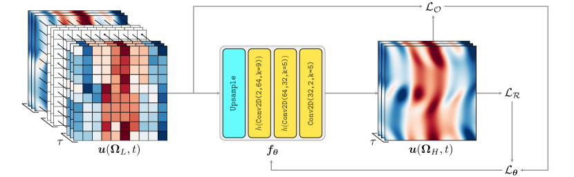
Figure 1: Super-resolution task. The model ${\bm{f_{\theta}}}$ is responsible for mapping the low-resolution field ${\bm{u}}({\bm{\Omega}_{L}},t)$ to the high-resolution field ${\bm{u}}({\bm{\Omega}_{H}},t)$. The upsampling layers (middle white layers in the leftmost set of data) perform bi-cubic upsampling to obtain the correct spatial dimensions. Convolutional layers are parameterised as Conv2D(c_in, c_out, k)|, where c_in, c_out| denote the number of input and output channels, respectively; and k| is the spatial extent of the filter. The terms $\mathcal{L}_{\mathcal{O}},\mathcal{L}_{\mathcal{R}}$ denote the observation-based loss and residual loss, respectively, the combination of which forms the objective loss $\mathcal{L}_{\bm{\theta}}$, which is used to update the network’s parameters, ${\bm{\theta}}$. We provide an in-depth explanation of these losses in §4.

For this, we propose a super-resolution method that does not require the full set of high-resolution observations. To accomplish this, we design and propose the physics-constrained convolutional neural network (PC-CNN) with a time windowing scheme. We apply this to a two-dimensional chaotic and turbulent fluid motion. The paper is structured as follows. In §2 we introduce the super-resolution task in the context of a mapping from low- to high- resolution. The choice of architecture used to represent the mapping is discussed in §3 before providing an overview of the methodology §4. We introduce the two-dimensional, turbulent flow in §5 and provide details on the pseudospectral method used for discretisation. Finally, results are demonstrated in §6. Conclusions §7 end the paper.

2 Super-resolution task

We consider partial differential equations (PDEs) of the form

$$\mathcal{R}({\bm{\tilde{u}}};\lambda)\equiv\partial_{t}{\bm{\tilde{u}}}-\mathcal{N}({\bm{\tilde{u}}};\lambda),$$ (1)

where ${\bm{x}}\in\Omega\subset\mathbb{R}^{n}$ denotes the spatial location; $t\in[0,T]\subset\mathbb{R}_{\geq 0}$ is the time, where $n$ is the space dimension; ${\bm{\tilde{u}}}:\Omega\times[0,T]\rightarrow\mathbb{R}^{m}$ is the state, where where $m$ is the number of components of the vector function ${\bm{\tilde{u}}}$; $\lambda$ are the physical parameters of the system; $\mathcal{N}$ is a sufficiently smooth differential operator, which represents the nonlinear part of the system of $m$ partial differential equations; $\mathcal{R}$ is the residual; and $\partial_{t}$ is the partial derivative with respect to time. A solution ${\bm{u}}$ of the PDE (1) is the function that makes the residual vanish, i.e., $\mathcal{R}({\bm{u}};\lambda)=0$.

Given sparse observations, ${\bm{u}}({\bm{\Omega}_{L}},t)$, we aim to reconstruct the underlying solution to the partial differential equation on a high-resolution grid, ${\bm{u}}({\bm{\Omega}_{H}},t)$, where the domain $\Omega$ is discretised on low- and high-resolution uniform grids, ${\bm{\Omega}_{L}}\subset\mathbb{R}^{N^{n}}$ and ${\bm{\Omega}_{H}}\subset\mathbb{R}^{M^{n}}$, respectively, such that ${\bm{\Omega}_{L}}\cap{\bm{\Omega}_{H}}={\bm{\Omega}_{L}}$; $M=\kappa N$; and $\kappa\in\mathbb{N}^{+}$ is the up-sampling factor. Our objective is to find a parameterised mapping ${\bm{f_{\theta}}}$ such that

$${\bm{f_{\theta}}}:{\bm{u}}({\bm{\Omega}_{L}},t)\rightarrow{\bm{u}}({\bm{\Omega}_{H}},t).$$ (2)

We consider the solution, ${\bm{u}}$, to be discretised with $N_{t}$ times steps, $t_{i}$, which are contained in the set $\mathcal{T}=\{t_{i}\in[0,T]\}_{i=0}^{N_{t}}$. We approximate the mapping ${\bm{f_{\theta}}}$ by a convolutional neural network parameterised by ${\bm{\theta}}$.

3 Convolutional neural networks

Parameterising ${\bm{f_{\theta}}}$ as a convolutional neural network is a design choice, which allows us to exploit two key properties. First, shift invariance, which is consequence of kernel-based operations acting on structured grids [14]. Second, partial differential equations are defined by local operators, which is a property that we wish the machine to induce naturally. Therefore, we choose convolutional neural networks, which employ an architectural paradigm that leverages spatial correlations [15], through the composition of functions

$${\bm{f_{\theta}}}={\bm{f}}^{Q}_{\bm{\theta}_{Q}}\circ\cdots\circ h({\bm{f}}^{1}_{\bm{\theta}_{1}})\circ h({\bm{f}}^{0}_{\bm{\theta}_{0}}),$$ (3)

where ${\bm{f}}^{i}_{{\bm{\theta}}_{i}}$ denote discrete convolutional layers; $h$ is an element-wise nonlinear activation function, which increases the expressive power of the network [e.g., 16] and yields a universal function approximator [17]; and $Q$ is the number of layers. The convolutional layers are responsible for the discrete operation $({\bm{x}},\bm{w},\bm{b})\mapsto{\bm{w}}\ast{\bm{x}}+{\bm{b}}$, where ${\bm{\theta}}=({\bm{w}},{\bm{b}})$. As the kernel operates locally around each pixel, information is leveraged from the surrounding grid cells. This makes convolutional layers an excellent choice for learning and exploiting spatial correlations, as are often important in the solutions to partial differential equations [e.g., 18, 13].

We propose a physics-constrained convolutional neural network (PC-CNN), which consists of three successive convolutional layers that are prepended by an upsampling operation tasked with increasing the spatial resolution of the input. Knowledge of the boundary conditions can be imposed through the use of padding; for instance periodic padding for periodic boundary conditions. Figure 1 provides an overview of the super-resolution task with information about the architecture employed.

4 Methodology

Having defined the mapping ${\bm{f_{\theta}}}$ as a convolutional neural network parameterised by ${\bm{\theta}}$, we formalise an optimisation problem to minimise the cost function $\mathcal{L}_{\bm{\theta}}$

$${\bm{\theta}}^{\ast}=\operatorname*{argmin}_{\bm{\theta}}\mathcal{L}_{\bm{\theta}}\quad\text{where}\quad\mathcal{L}_{\bm{\theta}}=\mathcal{L}_{\mathcal{O}}+\alpha\mathcal{L}_{\mathcal{R}},$$ (4)

where $\alpha$ is a non-negative empirical regularisation factor, which determines the relative importance of the corresponding loss terms. Given low-resolution observations ${\bm{u}}({\bm{\Omega}_{L}},t)$ at arbitrary times $t\in\mathcal{T}$, we define each of the loss terms as

$$\mathcal{L}_{\mathcal{O}} =\frac{1}{N_{t}}\sum_{t\in\mathcal{T}}\lVert{\left.\kern-1.2pt{\bm{f_{\theta}}}({\bm{u}}({\bm{\Omega}_{L}},t))\vphantom{\big{|}}\right|^{{\bm{\Omega}_{L}}}}-{\bm{u}}({\bm{\Omega}_{L}},t)\rVert_{{\bm{\Omega}_{L}}}^{2},$$ (5)

$$\mathcal{L}_{\mathcal{R}} =\frac{1}{N_{t}}\sum_{t\in\mathcal{T}}\lVert\mathcal{R}({\bm{f_{\theta}}}({\bm{u}}({\bm{\Omega}_{L}},t));\lambda)\rVert_{{\bm{\Omega}_{H}}}^{2},$$

where ${\left.\kern-1.2pt{\bm{f_{\theta}}}(\mathrel{\;\cdot\;})\vphantom{\big{|}}\right|^{{\bm{\Omega}_{L}}}}$ denotes the corestriction of ${\bm{\Omega}_{H}}$ on ${\bm{\Omega}_{L}}$, and $\lVert\mathrel{\;\cdot\;}\rVert_{\bm{\Omega}}$ represents the $\ell^{2}$-norm over the domain ${\bm{\Omega}}$. In order to find an optimal set of parameters ${\bm{\theta}}^{\ast}$, the loss is designed to regularise predictions that do not conform to the desired output. Given sensor observations ${\bm{u}}({\bm{\Omega}_{L}},t)$ in the low-resolution input, the observation-based loss, $\mathcal{L}_{\mathcal{O}}$, is defined to minimise the distance between known observations, ${\bm{u}}({\bm{\Omega}_{L}},t)$, and their corresponding predictions on the high-resolution grid, ${\bm{f_{\theta}}}({\bm{u}}({\bm{\Omega}_{L}},t))$.

We impose the prior knowledge that we have on the dynamical system by defining the residual loss, $\mathcal{L}_{\mathcal{R}}$, which penalises the parameters that yield predictions that violate the governing equations (1). Mathematically, this means that weIn absence of observations (i.e., data), the residual loss $\mathcal{L}_{\mathcal{R}}$ alone does not provide a unique solution. By augmenting the residual loss with the data loss, $\mathcal{L}_{\mathcal{O}}$ (see Eq. (4)), we ensure that network realisations conform to the observations (data) whilst fulfilling the governing equations, e.g., conservation laws. Crucially, as consequence of the proposed training objective, we do not need the high-resolution field as labelled dataset, which is required with conventional super-resolution methods.

4.1 Time-windowing of the residual loss

Computing the residual of a partial differential equation is a temporal task, as shown in Eq. (1). We employ a time-windowing approach to allow the network ${\bm{f_{\theta}}}$ to learn the sequentiality of the data. This provides a means to compute the time-derivative $\partial_{t}{\bm{u}}$ required for the residual loss $\mathcal{L}_{\mathcal{R}}$. The network takes time-windowed samples as inputs, each sample consisting of $\tau$ sequential time-steps. The time-derivative $\partial_{t}{\bm{u}}$ is computed by applying a forward Euler approximation to the loss

$$\begin{split}\mathcal{L}_{\mathcal{R}}=\frac{1}{\tau N_{t}}\sum_{t\in\mathcal{T}}\sum_{n=0}^{\tau}\big{\lVert}\partial_{t}{\bm{f_{\theta}}}({\bm{u}}({\bm{\Omega}_{L}},t+n\Delta t))\\ -\mathcal{N}({\bm{f_{\theta}}}({\bm{u}}({\bm{\Omega}_{L}},t+n\Delta t));\lambda)\big{\rVert}_{{\bm{\Omega}_{H}}}^{2}.\end{split}$$ (6)

Using this approach, we are able to obtain the residual for the predictions in a temporally local sense; computing derivatives across discrete time windows rather than the entire simulation domain. The network ${\bm{f_{\theta}}}$ is augmented to operate on these time windows, which vectorises the operations over the time-window. For a fixed quantity of training data, the choice of $\tau$ introduces a trade-off between the number of input samples $N_{t}$, and the size of each time-window $\tau$. We take a value $\tau=2$, which is the minimum window size for computing the residual loss $\mathcal{L}_{\mathcal{R}}$. We find that this is sufficient for training the network whilst simultaneously maximising the number of independent samples used for training. To avoid duplication of the data in the training set, we ensure that all samples are at least $\tau$ time-steps apart so that independent time-windows are guaranteed to not contain any overlaps.

5 Chaotic and turbulent dataset

As nonlinear partial differential equations, we consider the Navier-Stokes equations, which are the expressions of the conservation of mass and momentum of fluid motion, respectively

$$\begin{split}\nabla\cdot{\bm{u}}&=0,\\ \partial_{t}{\bm{u}}+\left({\bm{u}}\cdot\bm{\nabla}\right){\bm{u}}&=-\nabla p+\nu\Delta{\bm{u}}+\bm{g},\end{split}$$ (7)

where $p,\nu$ denote the scalar pressure field and kinematic viscosity, respectively. The flow velocity, ${\bm{u}}\in\mathbb{R}^{m=2}$ evolves on the domain $\Omega\in[0,2\pi)\subset\mathbb{R}^{n=2}$ with periodic boundary conditions applied on $\partial\Omega$, and a stationary, spatially-varying sinusoidal forcing term ${\bm{g}}({\bm{x}})$. In this paper, we take $\nu=\nicefrac{{1}}{{42}}$ to ensure chaotic and turbulent dynamics, and employ the forcing term ${\bm{g}}({\bm{x}})=\left[\sin{(4\bm{x_{2}}),0}\right]^{\top}$ [19], where $\bm{x_{2}}$ is the transverse coordinate. This flow, which is also known as the Kolmogorov flow [19], provides a nonlinear and multi-scale dateset, which allows us to evaluate the quality of predictions across the turbulent spectrum.

5.1 Differentiable pseudospectral discretisation

To produce a solution for the Kolmogorov flow, we utilise a differentiable pseudospectral spatial discretisation $\bm{\hat{\bm{u}}}_{k}=\hat{\bm{u}}({\bm{k}},t)$ where $\hat{\bm{u}}=\mathcal{F}\circ{\bm{u}}$; $\mathcal{F}$ is the Fourier transform; and ${\bm{k}}\in\hat{\bm{\Omega}}_{k}\subset\mathbb{C}^{K^{n}}$ is the spectral discretisation of the spatial domain $\Omega\in[0,2\pi)$ [20]. Operating in the Fourier domain eliminates the continuity term [21]. The equations for the spectral representation of the Kolmogorov flow are

$$\mathcal{R}(\bm{\hat{\bm{u}}}_{k};\lambda)=\left(\tfrac{d}{dt}+\nu\lvert{\bm{k}}\rvert^{2}\right)\bm{\hat{\bm{u}}}_{k}-{\bm{\hat{f}}}_{k}+{\bm{k}}\frac{{\bm{k}}\cdot{\bm{\hat{f}}}_{k}}{\lvert{\bm{k}}\rvert^{2}}-{\hat{\bm{g}}}_{k},$$ (8)

with ${\bm{\hat{f}}}_{k}=-\left(\widehat{{\bm{u}}\cdot\nabla{\bm{u}}}\right)_{k}$, where nonlinear terms are handled pseudospectrally, employing the $\nicefrac{{2}}{{3}}$ de-aliasing rule to avoid unphysical culmination of energy at the high frequencies [21]. A solution is produced by time-integration of the dynamical system with the explicit forward-Euler scheme, choosing a time-step $\Delta t$ that satisfies the Courant-Friedrichs-Lewy (CFL) condition. Initial conditions are generated by producing a random field scaled by the wavenumber, which retains the spatial structures of varying lengthscale in the physical domain [22]. The initial transient, which is approximately $T_{t}=180s$, is removed from the dataset to ensure that the results are statistically stationary. (The transient time is case dependant.) For a spatial resolution ${\bm{\Omega}_{H}}\in\mathbb{R}^{70\times 70}$, we use a spectral discretisation $\hat{\bm{\Omega}}_{k}\in\mathbb{C}^{35\times 35}$ to avoid aliasing and resolve the smallest lengthscales possible.

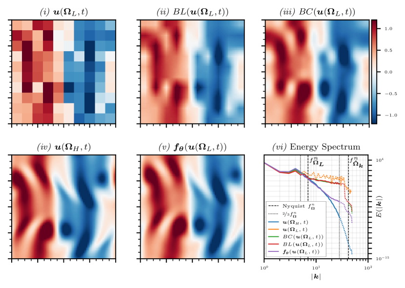
Figure 2: Super-resolution results. Physics-constrained convolutional neural network (PC-CNN) compared with interpolation methods. Panel (i) shows the low-resolution input, ${\bm{u}}({\bm{\Omega}_{L}},t)$; (ii) bi-linear interpolation, $\textit{BL}({\bm{u}}({\bm{\Omega}_{L}},t))$; (iii) bi-cubic interpolation, $\textit{BC}({\bm{u}}({\bm{\Omega}_{L}},t))$; (iv) true high-resolution field, ${\bm{u}}({\bm{\Omega}_{H}},t)$; (v) model prediction of the high-resolution field, ${\bm{f_{\theta}}}({\bm{u}}({\bm{\Omega}_{L}},t))$; and (vi) energy spectra for each of the predictions.

5.2 Residual loss in the Fourier domain

The pseudospectral discretisation provides an efficient means to compute the differential operator $\mathcal{N}$, which allows us to evaluate the residual loss $\mathcal{L}_{\mathcal{R}}$ in the Fourier domain

$$\begin{split}\mathcal{L}_{\mathcal{R}}=\frac{1}{\tau N_{t}}\sum_{t\in\mathcal{T}}\sum_{n=0}^{\tau}\lVert\partial_{t}\hat{\bm{f_{\theta}}}({\bm{u}}({\bm{\Omega}_{L}},t+n\Delta t))\\ -\hat{\mathcal{N}}(\hat{\bm{f_{\theta}}}({\bm{u}}({\bm{\Omega}_{L}},t+n\Delta t)))\rVert_{\bm{\hat{\Omega}_{k}}}^{2},\end{split}$$ (9)

where $\hat{\bm{f_{\theta}}}=\mathcal{F}\circ{\bm{f_{\theta}}}$, and $\hat{\mathcal{N}}$ denotes the Fourier-transformed differential operator. The pseudospectral discretisation is fully differentiable, which allows us to numerically compute gradients with respect to the parameters of the network ${\bm{f_{\theta}}}$. Computing the loss $\mathcal{L}_{\mathcal{R}}$ in the Fourier domain provides two advantages: (i) periodic boundary conditions are naturally enforced, which enforces the prior knowledge in the loss calculations; and (ii) gradient calculations yield spectral accuracy. In contrast, a conventional finite differences approach requires a computational stencil, the spatial extent of which places an error bound on the gradient computation. This error bound is a function of the spatial resolution of the field.

6 Results

First, we discuss the generation of the low-resolution data for the super-resolution task. Next, we show the ability of the PC-CNN to infer the high-resolution solution of the partial differential equation on points that are not present in the training set.

6.1 Obtaining the low-resolution data

A high-resolution solution of the partial differential equation is generated on the grid ${\bm{\Omega}_{H}}$ prior to extracting a low-resolution grid ${\bm{\Omega}_{L}}$ with the downsampling factor of $\kappa=\nicefrac{{N}}{{M}}$. Both the solver and residual loss are discretised with $K=\nicefrac{{N}}{{2}}$ wavenumbers in the Fourier domain, which complies with the Nyquist-Shannon sampling criterion. The downsampling by $\kappa$ is performed by extracting the value of the solution at spatial locations ${\bm{\Omega}_{L}}\cap{\bm{\Omega}_{H}}$, i.e., a low-resolution representation of the high-resolution solution

$${\bm{u}}({\bm{\Omega}_{L}},t)\triangleq{\left.\kern-1.2pt{\bm{u}}({\bm{\Omega}_{H}},t)\vphantom{\big{|}}\right|^{{\bm{\Omega}_{L}}}}.$$ (10)

(In contrast, the use of a pooling method for downsampling would distort values in the low-resolution representation, which effectively modifies the high-resolution solution.)

6.2 Comparison with standard upsampling

We showcase the results for a downsampling factor $\kappa=7$. Results are compared with interpolating upsampling methods, i.e., bi-linear, and bi-cubic interpolation to demonstrate the ability of the method. We provide a notion of quantitative accuracy by computing the relative $\ell^{2}$-error between the true solution, ${\bm{u}}({\bm{\Omega}_{H}},t)$, and the corresponding network realisation, ${\bm{f_{\theta}}}({\bm{u}}({\bm{\Omega}_{L}},t))$

$$e=\sqrt{\frac{\sum_{t\in\mathcal{T}}\lVert{\bm{u}}(\bm{\Omega_{H}},t)-{\bm{f_{\theta}}}({\bm{u}}(\bm{\Omega_{L}},t))\rVert_{\bm{\Omega_{H}}}^{2}}{\sum_{t\in\mathcal{T}}\lVert{\bm{u}}(\bm{\Omega_{H}},t)\rVert_{\bm{\Omega_{H}}}^{2}}}.$$ (11)

Upon discarding the transient, a solution ${\bm{u}}({\bm{\Omega}_{H}},t)\in\mathbb{R}^{70\times 70}$ is generated by time-integration over $12\times 10^{3}$ time-steps, with $\Delta t=1\times 10^{-3}$. We extract the low-resolution solution ${\bm{u}}({\bm{\Omega}_{L}},t)\in\mathbb{R}^{10\times 10}$ as a candidate for the super-resolution task. We extract $2048$ samples at random from the time-domain of the solution, each sample consisting of $\tau=2$ consecutive time-steps. The adam optimiser [23] is employed for training with a learning rate of $3\times 10^{-4}$. We take $\alpha=10^{3}$ as the regularisation factor for the loss $\mathcal{L}_{\bm{\theta}}$ and train for a total of $10^{3}$ epochs, which is empirically determined to provide sufficient convergence.

Figure 2 shows a snapshot of results for the streamwise component of the velocity field, comparing network realisations ${\bm{f_{\theta}}}({\bm{u}}({\bm{\Omega}_{L}},t))$ with the interpolated alternatives. Bi-linear and bi-cubic interpolation are denoted by $BL({\bm{u}}({\bm{\Omega}_{L}},t)),BC({\bm{u}}({\bm{\Omega}_{L}},t))$ respectively. We observe that network realisations of the high-resolution solution yield qualitatively more accurate results as compared with the interpolation. Artefacts indicative of the interpolation scheme used are present in both of the interpolated fields, whereas the network realisation captures the structures present in the high-resolution field correctly. Across the entire solution domain the model ${\bm{f_{\theta}}}$ achieves a relative $\ell^{2}$-error of $e=3.449\times 10^{-2}$ compared with $e=2.091\times 10^{-1}$ for bi-linear interpolation and $e=1.717\times 10^{-1}$ for bi-cubic interpolation.

Although the relative $\ell^{2}$-error provides a notion of predictive accuracy, it is crucial to assess the physical characteristics of the super-resolved field [24]. The energy spectrum, which is characteristic of turbulent flows, represents a multi-scale phenomenon where energy content decreases with the wavenumber. From the energy spectrum of the network’s prediction, ${\bm{f_{\theta}}}({\bm{u}}(\bm{\Omega}_{L},t))$, we gain physical insight into the multi-scale nature of the solution. Results in Figure 2 show that the energy content of the low-resolution field diverges from that of the high-resolution field, which is a consequence of spectral aliasing. Network realisations ${\bm{f_{\theta}}}({\bm{u}}({\bm{\Omega}_{L}},t))$ are capable of capturing finer scales of turbulence compared to both interpolation approaches, prior to diverging from the true spectrum as $\lvert{\bm{k}}\rvert=18$. The residual loss, $\mathcal{L}_{\mathcal{R}}$, enables the network to act beyond simple interpolation. The network is capable of de-aliasing, thereby inferring unresolved physics. Parametric studies show similar results across a range of super-resolution factors $\kappa$ (result not shown).

7 Conclusions

In this paper, we introduce a method for physics-constrained super-resolution of observations in partial differential equations without access to the full high-resolution samples. First, we define the super-resolution task and introduce the physics-constrained convolutional neural network (PC-CNN), which provides the framework to compute physical residuals for spatiotemporal systems. Second, we formulate an optimisation problem by leveraging knowledge of the partial differential equations and low-resolution observations to regularise the predictions from the network. Third, we showcase the PC-CNN on a turbulent flow, which is a spatiotemporally chaotic solution of the nonlinear partial differential equations of fluid motion (Navier-Stokes). Finally, we demonstrate that the proposed PC-CNN provides more accurate physical results, both qualitatively and quantitatively, as compared to interpolating upsampling methods. This work opens opportunities for the accurate reconstruction of solutions of partial differential equations from sparse observations, as is prevalent in experimental settings, without the full set of high-resolution images.

8 Acknowledgements

D. Kelshaw. and L. Magri. acknowledge support from the UK Engineering and Physical Sciences Research Council. L. Magri gratefully acknowledges financial support from the ERC Starting Grant PhyCo 949388.

References

- Brunton et al. [2016] S. L. Brunton, J. L. Proctor, and J. N. Kutz, “Discovering governing equations from data by sparse identification of nonlinear dynamical systems,” Proceedings of the National Academy of Sciences, vol. 113, no. 15, pp. 3932–3937, 2016.
- Dong et al. [2014] C. Dong, C. C. Loy, K. He, and X. Tang, “Learning a deep convolutional network for image super-resolution,” in European Conference on Computer Vision, 2014, pp. 184–199.
- Shi et al. [2016] W. Shi, J. Caballero, F. Huszár, J. Totz, A. P. Aitken, R. Bishop, D. Rueckert, and Z. Wang, “Real-time single image and video super-resolution using an efficient sub-pixel convolutional neural network,” Proceedings of the IEEE Conference on Computer Vision and Pattern Recognition (CVPR), 9 2016.
- Yang et al. [2019] W. Yang, X. Zhang, Y. Tian, W. Wang, J.-H. Xue, and Q. Liao, “Deep learning for single image super-resolution: A brief review,” IEEE Transactions on Multimedia, vol. 21, pp. 3106–3121, 12 2019.
- Liu et al. [2020] B. Liu, J. Tang, H. Huang, and X.-Y. Lu, “Deep learning methods for super-resolution reconstruction of turbulent flows,” Physics of Fluids, vol. 32, p. 25105, 2020.
- Lagaris et al. [1998] I. E. Lagaris, A. Likas, and D. I. Fotiadis, “Artificial neural networks for solving ordinary and partial differential equations,” IEEE Transactions on Neural Networks, vol. 9, pp. 987–1000, 1998.
- Raissi et al. [2019] M. Raissi, P. Perdikaris, and G. E. Karniadakis, “Physics-informed neural networks: A deep learning framework for solving forward and inverse problems involving nonlinear partial differential equations,” Journal of Computational Physics, vol. 378, pp. 686–707, 2 2019.
- Doan et al. [2021] N. Doan, W. Polifke, and L. Magri, “Short-and long-term predictions of chaotic flows and extreme events: a physics-constrained reservoir computing approach,” Proceedings of the Royal Society A, vol. 477, no. 2253, p. 20210135, 2021.
- Eivazi and Vinuesa [2022] H. Eivazi and R. Vinuesa, “Physics-informed deep-learning applications to experimental fluid mechanics,” 2022. [Online]. Available: https://arxiv.org/abs/2203.15402
- Krishnapriyan et al. [2021] A. Krishnapriyan, A. Gholami, S. Zhe, R. Kirby, and M. W. Mahoney, “Characterizing possible failure modes in physics-informed neural networks,” Advances in Neural Information Processing Systems, vol. 34, pp. 26 548–26 560, 2021.
- Grossmann et al. [2023] T. G. Grossmann, U. J. Komorowska, J. Latz, and C.-B. Schönlieb, “Can physics-informed neural networks beat the finite element method?” arXiv preprint arXiv:2302.04107, 2023.
- Kelshaw and Magri [2023] D. Kelshaw and L. Magri, “Uncovering solutions from data corrupted by systematic errors: A physics-constrained convolutional neural network approach,” 2023.
- Gao et al. [2021] H. Gao, L. Sun, and J.-X. Wang, “Super-resolution and denoising of fluid flow using physics-informed convolutional neural networks without high-resolution labels,” Physics of Fluids, vol. 33, p. 073603, 7 2021.
- Gu et al. [2018] J. Gu, Z. Wang, J. Kuen, L. Ma, A. Shahroudy, B. Shuai, T. Liu, X. Wang, G. Wang, J. Cai, and T. Chen, “Recent advances in convolutional neural networks,” Pattern Recognition, vol. 77, pp. 354–377, 2018. [Online]. Available: https://www.sciencedirect.com/science/article/pii/S0031320317304120
- [15] Y. LeCun, Y. Bengio et al., “Convolutional networks for images, speech, and time series.”
- Magri [2023] L. Magri, “Introduction to neural networks for engineering and computational science,” 1 2023.
- Hornik et al. [1989] K. Hornik, M. Stinchcombe, and H. White, “Multilayer feedforward networks are universal approximators,” Neural Networks, vol. 2, pp. 359–366, 1989.
- Murata et al. [2020] T. Murata, K. Fukami, and K. Fukagata, “Nonlinear mode decomposition with convolutional neural networks for fluid dynamics,” Journal of Fluid Mechanics, vol. 882, p. A13, 2020.
- Fylladitakis [2018] E. D. Fylladitakis, “Kolmogorov flow: Seven decades of history,” Journal of Applied Mathematics and Physics, vol. 6, pp. 2227–2263, 2018.
- Kelshaw [2022] D. Kelshaw, “Kolsol,” https://github.com/magrilab/kolsol, 2022.
- Canuto et al. [1988] C. Canuto, M. Y. Hussaini, A. Quarteroni, and T. A. Zang, Spectral Methods in Fluid Dynamics. Springer Berlin Heidelberg, 1988.
- Ruan and McLaughlin [1998] F. Ruan and D. McLaughlin, “An efficient multivariate random field generator using the fast fourier transform,” Advances in Water Resources, vol. 21, no. 5, pp. 385–399, 1998.
- Kingma and Ba [2015] D. P. Kingma and J. Ba, “Adam: A method for stochastic optimization,” 2015.
- Pope and Pope [2000] S. B. Pope and Pope, Turbulent flows. Cambridge university press, 2000.