A VAE Approach to Sample Multivariate Extremes

Abstract

Generating accurate extremes from an observational data set is crucial when seeking to estimate risks associated with the occurrence of future extremes which could be larger than those already observed. Applications range from the occurrence of natural disasters to financial crashes. Generative approaches from the machine learning community do not apply to extreme samples without careful adaptation. Besides, asymptotic results from extreme value theory (EVT) give a theoretical framework to model multivariate extreme events, especially through the notion of multivariate regular variation. Bridging these two fields, this paper details a variational autoencoder (VAE) approach for sampling multivariate heavy-tailed distributions, i.e., distributions likely to have extremes of particularly large intensities. We illustrate the relevance of our approach on a synthetic data set and on a real data set of discharge measurements along the Danube river network. The latter shows the potential of our approach for flood risks’ assessment. In addition to outperforming the standard VAE for the tested data sets, we also provide a comparison with a competing EVT-based generative approach. On the tested cases, our approach improves the learning of the dependency structure between extremes.

Keywords: multivariate extreme value theory, variational auto-encoders, generative models, neural network, environmental risk

1 Introduction

Simulating samples from an unknown distribution is a task that various studies have successfully tackled in the machine learning (ML) community during the past decade. This has led to the emergence of generative algorithms, such as generative adversarial networks (GAN) (Goodfellow et al., 2020), VAEs (Kingma and Welling, 2013; Rezende et al., 2014), or normalizing flows (Rezende and Mohamed, 2015) (NF). As ML tasks usually focus on average behaviors rather than rare events, these methods were not tailored to generate extremes and extrapolate upon the largest value of the training data set. This is a major shortcoming when dealing with extremes. Risk assessment issues in worst-case scenarios imply to accurately sample extremes for large quantiles, which are beyond the largest value in observed data sets (Embrechts et al., 1999). We sketch in Figure 1 this problem for a two-dimensional problem case-study. Here, through a VAE approach, we aim to consistently generate samples in an extreme region (black square) from observations (blue dots) none of which belong to the extreme region. In this context, the EVT characterizes the probabilistic structure of extreme events and provides a theoretically-sound statistical framework to analyze them. Heavy-tail analysis (Resnick, 2007), in its broadest sense, is a branch of EVT that studies phenomena governed by multivariate power laws. Data modeled by heavy-tailed distributions cover a wide range of application fields, e.g., hydrology (Anderson and Meerschaert, 1998; Rietsch et al., 2013), particle motion (Fortin and Clusel, 2015), finance (Bradley and Taqqu, 2003), Internet traffic (Hernandez-Campos et al., 2004), and risk management (Chavez-Demoulin and Roehrl, 2004; Das et al., 2013). Recently, this area of research has gained some interest in the ML community.

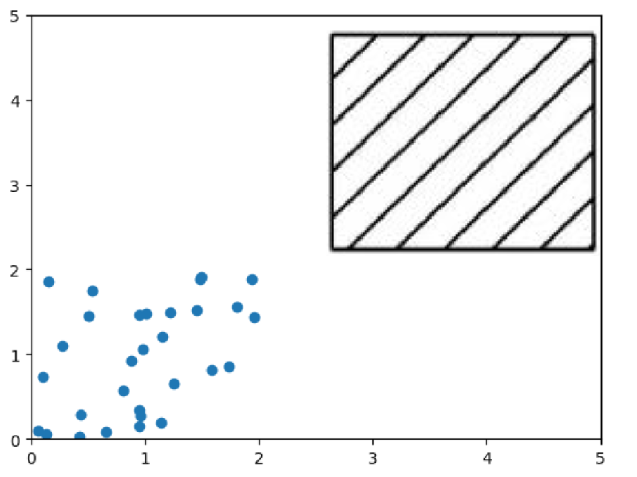
Figure 1: How to sample from observations (blue dots) in extreme regions (black square) to estimate probability of rare events?

Some work has shown the potential of bridging the gap between ML and EVT on different aspects, for example dimensionality reduction (Drees and Sabourin, 2021), quantile function approximation (Pasche and Engelke, 2022), outlier detection (Rudd et al., 2017), or classification in tail regions (Jalalzai et al., 2018). Concerning the generation of extremes, ML methods could also integrate EVT tools.

Related works: GANs and NFs have been applied to extreme sampling problems. As demonstrated in Jaini et al. (2020); Huster et al. (2021), the output random variable of a neural network associated with a light-tailed input random variable cannot be heavy-tailed. This has motivated previous works to adapt and extend to extremes. Regarding GANs, we can first distinguish GAN based on heavy-tailed priors, e.g. Feder et al. (2020) and Huster et al. (2021). Huster et al. (2021) proved that the mapping of a heavy-tailed random input variable by a large class of neural networks has the same extreme behavior as the input variable. In Boulaguiem et al. (2022), the proposed GAN exploit a copula-based parameterization (Embrechts, 2009) using Pareto distributions (see, e.g., Tencaliec et al., 2019) for the marginals, so that the GAN learns to sample multivariate distributions with uniform marginals. Another category of GAN schemes for extremes arise from the the observation that a neural network with rectified linear units (ReLU) cannot directly map the interval $[0,1]$ to the quantile function of a heavy-tailed law Allouche et al. (2022). This study then proposed a GAN to learn a transformation of this quantile function. The results demonstrated by Allouche et al. (2022) support the theoretical relevance of this GAN approximation for true quantile functions. A last category of GAN schemes proceeded empirically by recursively training GANs from tail samples up to the targeted return level Bhatia et al. (2021). Concerning NFs, Jaini et al. (2020) has also explored heavy-tailed latent variables using independent Student-t distributions. Extending this work, Laszkiewicz et al. (2022) proposed an approach which generate marginals with different tail behaviors.

Main contributions: To our knowledge, our study is the first attempt to bridge VAE and EVT. Recent studies suggest that state-of-the-art likelihood-based models, including VAEs, may, in some examples, capture the spread of the true distribution better than GANs (see, e.g., Razavi et al., 2019; Nash et al., 2021). This makes VAE an interesting way of explicitly exploiting the EVT framework to generate realistic and diverse extremes. Our main contributions are as follows.

• First, we demonstrate that VAE with standard parameterization cannot generate heavy-tailed distributions. Then, we propose a VAE framework to sample extremes from heavy-tailed distributions.

• The use of the multivariate EVT allows us to introduce the notion of angular measure which characterizes the asymptotic dependence between the extremes. Our approach allows to sample directly this angular measure thanks to a polar decomposition of the data. It allows us to better account for complex and non-singular distributions on the sphere for extremes, compared to other state-of-the-art generative schemes.

• Numerical experiments on both synthetic and real data sets support the relevance of our VAE scheme, including w.r.t. a EVT-based GAN approach (Huster et al., 2021). Especially, we demonstrate the ability to generate relevant samples beyond the largest values in the training data set.

Organization of the paper: This paper is organized as follows. We recall the basic principles of VAE and EVT in Section 2. In Section 3, we present our main theoretical results concerning, on the one hand, the tail distribution of the marginals generated by a VAE and, on the other hand, the angular measure of generative methods. All detailed proofs are delayed in Appendix G, listed in order of appearance in the paper. We detail the proposed VAE framework for multivariate extremes in Section 4 and describe the associated training setting in Section 5. Section 6 is dedicated to experiments. Section 7 is devoted to concluding remarks.

2 Background

In this section, we present background knowledge about VAE, and we give an introduction to univariate and multivariate heavy-tailed distributions.

2.1 Sampling with VAE

To generate a sample from a random variable $\bf X$, a VAE proposes a two-step sampling strategy:

• A sample $\mathbf{z}$ is drawn from a latent vector (or prior) $\mathbf{Z}$ with pdf $p_{\alpha}(\mathbf{z})$ (possibly) parameterized by $\alpha$;

• The desired sample is obtained by sampling from the conditional pdf $p(\mathbf{x}\mid\mathbf{z})$.

Since $p(\mathbf{x}\mid\mathbf{z})$ is in general not known, one uses a parametric approximation $p_{\theta}(\mathbf{x}\mid\mathbf{z})$, referred to as the likelihood or probabilistic decoder, with $\theta$ a set of parameters to be calibrated. The purpose is then to find the parameterization which enables to generate the most realistic samples of $\mathbf{X}$. To do so, VAE framework introduces a target distribution (or probabilistic encoder) $q_{\phi}(\mathbf{z}\mid\mathbf{x})$ parameterized by $\phi$ to approximate the true posterior distribution. The training phase then comes to maximize the evidence lower bound (ELBO) with respect to the set of parameters $(\alpha,\phi,\theta)$. Formally, given $N$ independent samples $(\mathbf{x}^{(i)})_{i=1}^{N}$ of $\bf X$, we have

$$-\log(p(\mathbf{x}^{(i)})\geq L(\mathbf{x}^{(i)},\alpha,\theta,\phi),$$

with $L$ the ELBO cost given by

$$L(\mathbf{x}^{(i)},\alpha,\theta,\phi)=-D_{KL}\left(q_{\phi}(\mathbf{z}\mid\mathbf{x}^{(i)})\mid\mid p_{\alpha}(\mathbf{z})\right)+E_{q_{\phi}(\mathbf{z}\mid\mathbf{x}^{(i)})}\left[\log p_{\theta}(\mathbf{x}^{(i)}\mid\mathbf{z})\right].$$ (1)

The ELBO cost on the whole data set is obtained by averaging Equation (1) over the $N$ samples of $\mathbf{X}$. To infer the set of parameters $(\alpha,\phi,\theta)$ by neural network functions of the data, Kingma and Welling (2013) and Rezende et al. (2014) derived a specific training scheme for ELBO optimization. The authors allowed the cost function defined by Equation (1) to be approximated by an unbiased Monte Carlo estimator differentiable with respect to both $\theta$ and $\phi$. This Monte Carlo estimator is given for a data point by

$$\hat{L}(\mathbf{x}^{(i)},\alpha,\theta,\phi)=-D_{KL}\left(q_{\phi}(\mathbf{z}\mid\mathbf{x}^{(i)})\mid\mid p_{\alpha}(\mathbf{z})\right)+\frac{1}{L}\sum_{l=1}^{L}\log p_{\theta}(\mathbf{x}^{(i)}\mid\mathbf{z}^{(i,l)}),$$ (2)

where $\mathbf{z}^{(i,l)}$ are samples from the approximate posterior $q_{\phi}(\mathbf{z}\mid\mathbf{x}^{(i)})$. To make this expression differentiable, we have to exploit a reparameterization trick. It comes to find a function $g_{\phi}$, such that

$$q_{\phi}(\mathbf{z}\mid\mathbf{x})=g_{\phi}(\mathbf{x},\mathbf{\epsilon}),$$ (3)

with $\epsilon$ a chosen random variable, and $g_{\phi}$ differentiable with respect to $\phi$. When explicit reparameterization is not feasible, we may exploit implicit reparameterization gradients (see Figurnov et al., 2018). Details about implicit reparameterization can be found in Appendix F.

Example 1

The most common parameterization of a VAE with ${\bf z}\in\mathbb{R}^{n}$ and ${\bf x}\in\mathbb{R}^{m}$ is

$$p({\bf z}) =\mathcal{N}({\bf z}\ ;\ {\bf 0},{\bf I}_{n}),$$

$$p_{\theta}({\bf x}\mid{\bf z}) =\mathcal{N}\left({\bf x}\ ;\ {\bf\mu}_{\theta}({\bf z}),\operatorname{diag}({\bf\sigma}_{\theta}({\bf z}))^{2}\right),$$

$$q_{\phi}({\bf z}\mid{\bf x}) =\mathcal{N}\left({\bf z}\ ;\ {\bf\mu}_{\phi}({\bf x}),\operatorname{diag}({\bf\sigma}_{\phi}({\bf x}))^{2}\right),$$

where $\operatorname{diag}$ is the operator that produces a diagonal matrix whose diagonal elements are the elements of the input vector, and $\mathcal{N}({\bf z}\ ;\ {\bf\mu},{\bf\Sigma})$ denotes the pdf in $\bf z$ of the multivariate normal distribution of mean $\mu$ and covariance matrix $\Sigma$. In this framework, the reparametrization trick is given by

$$g_{\phi}(\mathbf{x},\mathbf{\epsilon})={\bf\mu}_{\phi}({\bf x})+{\bf\sigma}_{\phi}({\bf x})\odot\epsilon,$$

where $\epsilon$ is sampled from the centered isotropic multivariate Gaussian $\mathcal{N}({\bf 0},I)$, and $\odot$ is the element-wise product. We refer to this parameterization as Standard VAE.

2.2 Univariate Extremes

When modelling univariate extremes, generalized Pareto (GP) (Pickands III, 1975) distributions are of great interest. The GP survival function is defined for $\xi\in\mathbb{R}$ and $\sigma>0$ by

$$\bar{H}_{\sigma,\xi}(x)=\left(1+\xi\frac{x}{\sigma}\right)_{+}^{-1/\xi},$$ (4)

where $a_{+}=0$ if $a<0$. The scalar $\xi$ is called the shape parameter. Note that Equation (4) is extended to $\xi=0$, with $\bar{H}_{\sigma,0}$ survival function of the exponential distribution of scale parameter $\sigma$.
Given a random variable $X$ with cdf $F$, GP distributions appear under mild condition as the simple limit of threshold exceedance function given by $F_{u}(x)=P(X-u\leq x\mid X>u)$ when $u\to\infty$ (Balkema and De Haan, 1974). To be explicit, under mild conditions there exists $\xi\in\mathbb{R}$ and a strictly positive function $\sigma(\cdot)$ such that

$$\lim_{u\to x_{F}}\sup_{0<x<x_{F}-u}\mid F_{u}(x)-H_{\sigma(u),\xi}(x)\mid=0,$$

with $x_{F}=\sup\{x\ \text{ s.t. }F(x)<1\}$ the right endpoint of $F$, and $H$ the cdf of the GP.
The shape parameter $\xi$ of the GP approximation of $F_{u}$ encompasses the information about the tail of $X$. In the following, we consider that:

• $\xi\leq 0$ corresponds to light-tailed distribution,

• $\xi>0$ corresponds to heavy-tailed distribution.

Remark 1

A simple yet efficient way to sample from a GP distribution with parameters $\xi$ and $\sigma$ is to multiply an inverse gamma distributed random variable with shape $\frac{1}{\xi}$ and rate $\sigma$ by a unit and independent exponential one. This multiplicative feature is essential for understanding the pivotal role of inverse-Gamma random variables in our sampling scheme in Section 4.1.

Remark 2

Notice that, given a light-tailed distribution with survival function $\bar{F}$, all its higher-order moments exist and are finite, and $\lim_{u\to\infty}u^{a}\bar{F}(u)=0$ for any $a>0$. In particular, Gaussian distribution is light-tailed. At the contrary, not all higher-order moments are finite for a heavy-tailed distribution.

In this work, we focus on heavy-tailed distributions, which can be seen as the distributions for which extremes have the greater intensity. The shape parameter characterizes how heavy is the tail of a distribution: the larger it is, the heavier the tail of the distribution.
A final important notion regarding extreme values is the so-called regular variation property.

Definition 3

A random variable $X$ is said to be regularly varying with tail index $\alpha>0$, if

$$\lim_{t\to+\infty}P(X>tx\ \mid\ X>t)=x^{-\alpha}.$$ (5)

Importantly, $X$ regularly varying equates to $X$ heavy-tailed with $\alpha=\frac{1}{\xi}$ (see Bingham et al., 1989, Theorem 8.13.2).

2.3 Multivariate Extremes

By extending notions developed in Section 2.2, a multivariate analogue of the GP distribution (Equation 4), referred to as multivariate GP, can be defined (see Rootzén and Tajvidi, 2006). Under mild conditions, exceedances distribution asymptotically follows multivariate GP distribution. Additionally, the regular variation of Definition 3 can be extended to a multivariate regular property (see, e.g. Resnick, 2007, for details). For a given random vector, the exceedances asymptotically have a multivariate GP distribution if the vector has multivariate regular variation.
Let $\mathbf{X}$ be a random vector in $\left(\mathbb{R}^{+}\right)^{m}$. To define multivariate regular variations, we decompose $\mathbf{X}$ into a radial component $R=X_{1}+\cdots+X_{m}=\|\mathbf{X}\|$ and an angular component of the $(m-1)$-dimensional simplex $\mathbf{\Theta}=\frac{\mathbf{X}}{\|{\bf X}\|}$.

Definition 4

$\bf X$ has multivariate regular variation if the two following properties are fulfilled:

• The radius $R$ is regularly varying as defined in Equation (5);

• There exists a probability measure $\mathbf{S}$ defined on the $(m-1)$-dimensional simplex such that $(R,\mathbf{\Theta})$ verifies

  $$P\left(\mathbf{\Theta}\in\bullet\bigm{|}R>r\right)\overset{w}{\longrightarrow}\mathbf{S}(\bullet),$$ (6)

  where $\overset{w}{\longrightarrow}$ denotes weak convergence (see Appendix B.2). $\bf S$ is called angular measure.

Consequently, the radius is a univariate heavy-tailed random variable as described in Section 2.2. Equation (6) indicates that, if the radius is above a sufficiently high threshold, the respective distributions of the radius and the angle can be considered independent. Estimating the angular measure then becomes crucial to address tail events of the kind of $\{\mathbf{X}\in C\}$ for an ensemble $C$ such that $u=\inf\{\|\mathbf{x}\|,\mathbf{x}\in C\}$ is large. This is especially true to assess the probability of joint extremes.
More generally, the estimation of the angular measure $\bf S$, although difficult due to the scarcity of examples (Clémençon et al., 2021), is of great interest for the analysis of extreme values. It allows, among other things, to determine confidence intervals for the probabilities of rare events (De Haan and De Ronde, 1998), bounds for probabilities of joint excesses over high thresholds (Engelke and Ivanovs, 2017) or tail quantile regions (Einmahl et al., 2013).

3 Tail properties of Distributions Sample by Generative Algorithms

This section is devoted to the theoretical foundations of the tail properties of distributions sampled by generative approaches in the machine learning community. We first stress in Section 3.1 that standard VAE cannot generate heavy-tailed marginals. Then we focus on angular measures that can be obtained using generative algorithms in Section 3.2. In particular, we prove that, when restricted to ReLU activation functions, generative algorithms based on the deterministic transformation of a prior input (e.g. GANs or NFs) have an angular measure concentrated on a restricted number of vectors. These theoretical considerations are crucial to define our VAE approach presented in Section 4.

3.1 Marginal Tail of a Standard VAE

In this section, we establish that a standard VAE only produces light-tailed marginals. This result extends to VAEs results similar to those established for GANs with normal prior (see Huster et al., 2021), or with NFs with light-tailed base distribution (Jaini et al., 2020). We first mention an important property of neural networks, based on the notion of Lipschitz continuity (see Appendix B.1).

Proposition 5

(Arora et al., 2016; Huster et al., 2021): A neural network $f:\mathbb{R}^{n}\rightarrow\mathbb{R}$ composed of operations such as ReLUs, leaky ReLUs, linear layers, maxpooling, maxout activation, concatenation or addition is a piecewise linear operator with a finite number of linear regions. Therefore, $f$ is Lipschitz continuous with respect to Minkowski distances.

Given these elements, the following proposition describes the tail of an univariate output of a stardard VAE.

Proposition 6

For the standard VAE of Example 1 with univariate output ($m=1$), given that the neural network functions $\mu_{\theta}$ and $\sigma_{\theta}$ of the probabilistic decoder are piecewise linear operators, then the output distribution sampled by the standard VAE is light-tailed.

Corollary 7

The marginal distributions generated by the standard VAE of Example 1 are light-tailed, whenever the neural networks functions $\mu_{\theta}$ and $\sigma_{\theta}$ neural networks are composed of operations described in Proposition 5.

3.2 Angular Measure of ReLu Networks Transformation of Random Vectors

In this section, we focus on the angular measures associated with generative algorithms. We demonstrate that distributions sampled by algorithms based on the transformation of a random input vector by a neural network with linear layers and ReLU activation functions have angular measures concentrated on finite set of points on the simplex. Although not specific to VAEs, these results suggest a particular focus on the representation of the angular measure in the VAE framework.
Let us consider the following framework for generating multivariate heavy-tailed data in the non-negative orthant:

$${\bf X}=f({\bf Z}),$$ (7)

with ${\bf Z}$ a $n$-dimensional input random vector with i.i.d heavy-tailed marginals and f a ReLU neural network which outputs in $\mathbb{R}^{m}$.
Generating through heavy-tailed input vector is used by Feder et al. (2020) and Huster et al. (2021) for GANs, and Jaini et al. (2020) for NFs. The marginals of the input vector have Pareto distribution in Huster et al. (2021), and t-Student in the others. As shown in Jaini et al. (2020), light-tailed marginals for the input vector lead to light-tailed marginals for the output. In the one-dimensional case, ${\bf X}$ is heavy-tailed with same shape parameter as ${\bf Z}$, whereas it has Gaussian tails whenever the input variable is Gaussian (Huster et al., 2021).
In the limit of extreme values, one can wonder what are the dependency structures between the marginals of ${\bf X}$ that such a model can represent. This corresponds to the angular measure defined in Equation (6). If we designate ${\bf S}_{\bf X}$ as the angular measure of ${\bf X}$, we can state the following Proposition.

Proposition 8

Under the framework described in Equation (7), ${\bf S}_{\bf X}$ is concentrated on a finite set of points of the simplex less than $n$. In other words, it means that there exist some vectors $\{{\bf v}_{1},{\bf v}_{2},\cdots,{\bf v}_{n^{\prime}}\}$ with $n^{\prime}\leq n$ such that for any subset $\mathbb{A}$ of the $(m-1)$-dimensional simplex

$${\bf S}_{\bf X}(\mathbb{A})=\sum_{i=1}^{n^{\prime}}p_{i}\delta_{{\bf v}_{i}}(\mathbb{A}),$$

where $\delta$ is the Dirac measure and $p_{i}>0$ such that $\sum_{i=1}^{n^{\prime}}p_{i}=1$.

Therefore, in the limit of infinite radius, ${\bf X}$ is almost surely located on a specific axis. While extracting certain principal directions in extreme regions is a useful tool for the comprehensive analysis of a data set (Drees and Sabourin, 2021), it is severely lacking in flexibility when it comes to represent more complex distributions and generate realistic extreme samples.
To circumvent this difficulty, we consider a polar decomposition, so we can generate the angle and the radius separately. Namely, we write ${\bf X}=(R,{\bf\Theta})$ as explained in Section 2.3. This allows to make explicit the dependency structure of the data whatever the radius is, especially for large radii. We can then obtain more varied angular measures than those concentrated on a finite number of vectors as illustrate in the numerical experiments reported in Section 6.

4 Proposed VAE Architecture

We propose the following three-step VAE scheme to generate a sample $\mathbf{x}^{(i)}$ of a multivariate regularly varying random vector:

• Using a VAE, a radius $r^{(i)}$ is drawn from a univariate heavy-tailed distribution $R$ (see Section 4.2);

• Conditionally on the drawn radius $r^{(i)}$, we sample $\mathbf{\Theta}^{(i)}$ an element of the $(m-1)$-dimensional simplex from the conditional distribution $\mathbf{\Theta}\mid[R=r^{(i)}]$ while forcing the independence between radius $R$ and angle $\mathbf{\Theta}$ for larger value of the radius. We use a conditional VAE for this purpose (see Section 4.3);

• We multiply compoment-wise the angle vector by the radius to obtain the desired sample, i.e. $\mathbf{x}^{(i)}=r^{(i)}\mathbf{\Theta}^{(i)}$.

The overall architecture is shown in Figure 2. As detailed in Section 3.2, the polar decomposition offers a great flexibility in modeling the dependence between variables, including for the angular measure, which is not the case for the transformation of heavy-tailed random vectors by ReLU networks (Proposition 8). Additionally, one can generate elements of the simplex with a given radius and study the dependence between variables at a given extreme level. The rest of this section details the architecture of the proposed VAE scheme chosen to sample the heavy-tailed radius and the conditional angle.

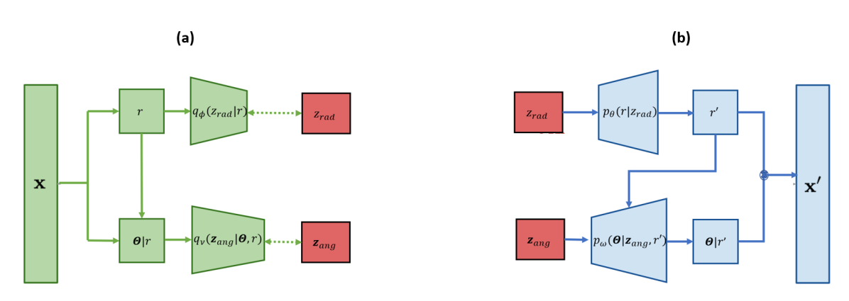
Figure 2: Global architecture of our approach with (a) the probabilistic encoders and (b) the probabilistic decoders. Ideally, distributions of $\bf x$ and ${\bf x}^{\prime}$ are similar. Solid arrows show a causal link between the different blocks. Dashed double arrows in (a) indicate that the distributions in the pointed blocks are compared using a Kullback-Leibler divergence criterion (Equation 2).

4.1 Idealized Multiplicative Framework for Sampling Heavy-tailed Radii

We model $R$ through a latent variable $Z_{rad}$. To deal with heavy-tailed distributions introduced in Section 2.2, we consider the following two conditions.

Condition 9

$Z_{rad}$ follows the inverse-gamma distribution defined by the pdf

$${\displaystyle f_{\bf Inv\Gamma}(z_{rad}\ ;\ \alpha,\beta)={\frac{\beta^{\alpha}}{\Gamma(\alpha)}}z_{rad}^{-\alpha-1}\exp\left(-\beta/z_{rad}\right)},$$ (8)

with $\alpha$ and $\beta$ two strictly positive constants, and $z_{r}ad>0$.

Condition 10

$R$ is linked to $Z_{rad}$ throughout a multiplicative model with a positive random coefficient $A$, i.e.

$$R\overset{\mathrm{d}}{=}A\times Z_{rad},$$

where $\overset{\mathrm{d}}{=}$ corresponds to a equality in distribution and the random variable $A$ is absolutely continuous and independent of $Z_{rad}$. We also assume that $0<E\left[A^{\alpha+\epsilon}\right]<\infty$ for some positive $\epsilon$.

We may recall that the inverse-gamma distribution is heavy-tailed with tail index $\alpha$ and has a strictly positive support. Above, moment condition $0<E\left[A^{\alpha+\epsilon}\right]<\infty$ means that $A$ has a significantly lighter tail than $Z_{rad}$.
Under these two conditions, Breiman’s lemma (Breiman, 1965) guarantees that the parameterization considered in Condition 10 leads to a heavy-tailed distribution of the radius $R$. Formally, the following proposition holds.

Proposition 11

If Conditions 9 and 10 hold, $R$ is heavy-tailed with tail index $\alpha$. In particular, if $A$ follows an exponential distribution with scale parameter $c$ then $R$ follows a GP distribution (see Equation 4 with $\xi=\frac{1}{\alpha}$ and $\sigma=\frac{\beta c}{\alpha}$)

4.2 Sampling from Heavy-tailed Radius Distributions

To tailor the VAE framework introduced in Section 2.1 to heavy-tailed random variables, we satisfy Condition 9, i.e. we set the prior $Z_{rad}$ as an inverse gamma distribution with parameters $\alpha$ and $\beta$. Notice that as if $Z_{rad}$ follows an inverse gamma distribution with parameters $\alpha$ and $\beta$, then for each $c>0$, $cZ_{rad}$ is an inverse gamma with parameters $\alpha$ and $c\beta$. Consequently, and without loss of generality, we set parameter $\beta$ of $Z_{rad}$ equal to $1$. Overall, we replace the light-tailed system described in Example 1 by the following heavy-tailed system:

$$p_{\alpha}(z_{rad}) =f_{\bf Inv\Gamma}(z_{rad}\ ;\ \alpha,1),$$ (9)

$$p_{\theta}(r\mid z_{rad}) =f_{\mathbf{\Gamma}}\left(r\ ;\ \alpha_{\theta}(z_{rad}),\beta_{\theta}(z_{rad})\right),$$ (10)

$$q_{\phi}(z_{rad}\mid r) =f_{\mathbf{Inv\Gamma}}\left(z_{rad}\ ;\ \alpha_{\phi}(r),\beta_{\phi}(r)\right),$$ (11)

with $f_{\mathbf{\Gamma}}$ (resp. $f_{\mathbf{Inv\Gamma}}$) the pdf of a Gamma (resp. inverse Gamma) distribution. $\alpha_{\theta}$, $\beta_{\theta}$, $\alpha_{\phi}$, $\beta_{\phi}$ are ReLU neural networks functions with parameters $\theta$ and $\phi$. We may stress that the above parameterization ensures the non-negativeness of the samples both for the target and the likelihood.
Following from the multiplicative framework described in Section 4.1, the following proposition holds regarding the heavy-tailed distributions of this univariate VAE scheme.

Proposition 12

We consider the VAE parameterization described by Equations (9), (10) and (11). If we further assume that the function $\alpha_{\theta}(.)$ is a strictly positive constant and the function $\beta_{\theta}(.)$ satisfies

$$\lim_{z_{rad}\to+\infty}\beta_{\theta}(z_{rad})\propto\frac{1}{z_{rad}},$$ (12)

$$\lim_{z_{rad}\to 0}\beta_{\theta}(z_{rad})\propto\frac{1}{z_{rad}},,$$ (13)

then the univariate output distribution sampled by this VAE scheme is heavy-tailed with tail index equal to $\alpha$.

In our implementation, we impose on $\beta_{\theta}(.)$ to satisfy Equations (12) and (13) by choosing

$$\beta_{\theta}(z_{rad})=\frac{|f_{\theta}(z_{rad})|}{z_{rad}^{2}},$$ (14)

where $f_{\theta}$ is a neural network with linear layers and ReLU activations.
Concerning $\alpha_{\theta}(.)$, we leave it in practice more flexible than a constant function. We only constrain a strictly positive finite limit at infinity. This corresponds to

$$\alpha_{\theta}(z_{rad})=\frac{|g_{\theta}(z_{rad})|}{z_{rad}},$$ (15)

where, again, $g_{\theta}$ is a neural network with linear layers and ReLU activations.
We choose our parameterization based on an anlogy with the ideal multiplicative framework described in Section 4.1. Indeed, considering Conditions 9 and 10 verified, then

$$R\mid[Z_{rad} =z_{rad}]\overset{\mathrm{d}}{=}Az_{rad},$$ (16)

$$Z_{rad}\mid[R =r]\overset{\mathrm{d}}{=}\frac{r}{A}.$$ (17)

As $A$ needs to have a tail lighter than $Z_{rad}$ to satisfy the moment condition $E\left[A^{\alpha+\epsilon}\right]<\infty$ for some positive $\epsilon$, we choose the approximate likelihood $p_{\theta}(r\mid z_{rad})$ in a light-tailed distribution family (i.e. Gamma distribution). Considering Equation (17), we notice that $Z_{rad}\mid[R=r]$ could be heavy-tailed if $A$ have non-null probability on each open set containing $0$. Thus we choose a heavy-tailed distribution for the target (i.e. Inverse-Gamma distribution). Additionally, as $R$ and $Z_{rad}$ are positive random variables, our parametrization ensures that negative values for either target and likelihood cannot occur.

Besides, by introducing the Inverse-Gamma parameterizations for the prior $p_{\alpha}$ and the target $q_{\phi}$ in Equation (2), we can derive an analytical expression of the ELBO cost of the proposed VAE.

Proposition 13

Given expression (9) and (11) for prior and target distributions, the KL divergence in Equation (2) is given by

$$D_{KL}\left(q_{\phi}(z_{rad}\mid r)\mid\mid p_{\alpha}(z_{rad})\right)=(\alpha_{\phi}(r)-\alpha)\psi(\alpha)-\log\frac{\Gamma(\alpha_{\phi}(r))}{\Gamma(\alpha)}$$

$$+\alpha\log\beta_{\phi}(r)+\alpha_{\phi}\frac{1-\beta_{\phi}(r)}{\beta_{\phi}(r)},$$ (18)

where $\Gamma$ and $\psi$ stands respectively for the gamma and digamma functions.

Interestingly, this proposition provides the basis for learning tail index $\alpha$ from data, which is a challenging issue in EVT (see, e.g. Danielsson et al., 2016).

4.3 Sampling on the Multivariate Simplex

The second component of our VAE scheme involves a conditional VAE (see, e.g., Zhao et al., 2017) to sample the angle conditionally on a previously sampled radius, namely conditional distribution ${\bf\Theta}\mid R$. This angular VAE with latent variable ${\bf Z}_{ang}$ exploits a multivariate normal prior. The target is also parameterized by multivariate normal distributions, with mean and standard deviation function of the hidden variable and of the observation data. The likelihood is parameterized by a projection of a normal distribution on the $\mathcal{L}_{1}$ sphere. Formally, let us denote by $\bf\Pi$ this projection such that, for any vector $\bf s$,

$$\bf\Pi({\bf s})=\frac{{\bf s}}{\|{\bf s}\|},$$

where the considered norm is the $\mathcal{L}_{1}$-norm. Additionally, we define ${\bf S}({\bf\Theta})=\{{\bf s},\ {\bf\Pi}({\bf s})={\bf\Theta}\}$. Overall, our conditional angular VAE relies on the following parameterization:

$$p({\bf z}_{ang}) =\mathcal{N}({\bf z}_{ang}\ ;{\bf 0},{\bf I}_{n}),$$

$$p_{\nu}({\bf\Theta}\mid{\bf z}_{ang},r) =\int_{{\bf S}({\bf\Theta})}\mathcal{N}\left({\bf s}\ ;\ {\bf\mu}_{\nu}({\bf z}_{ang},r),\operatorname{diag}({\bf\sigma}_{\nu}({\bf z}_{ang},r))^{2}\right),$$ (19)

$$q_{\omega}({\bf z}_{ang}\mid{\bf\Theta},r) =\mathcal{N}\left({\bf z}_{ang}\ ;\ {\bf\mu}_{\omega}({\bf\Theta},r),\operatorname{diag}({\bf\sigma}_{\omega}({\bf\Theta},r))^{2}\right),$$

where $n$ is the dimension of the latent space, ${\bf\mu}_{\nu}$, ${\bf\sigma}_{\nu}$, ${\bf\mu}_{\omega}$ and ${\bf\sigma}_{\omega}$ are neural network functions with parameters $\nu$ and $\omega$. The dependency on $R$ for the target and the likelihood has been made explicit to turn the framework conditional. Notice that we do not explicitly use Equation (4.3) when sampling from $p_{\nu}$, but we rather sample from $\mathcal{N}\left(\ {\bf\mu}_{\nu}({\bf z}_{ang},r),\operatorname{diag}({\bf\sigma}_{\nu}({\bf z}_{ang},r))^{2}\right)$ and then projecting on the sphere through $\bf\Pi$.
As our inital aim is to sample on the multivariate simplex rather than on the multivariate sphere, we also use a Dirichlet parameterization of the likelihood. Details regarding this parameterization can be found in Appendix C.
As we aim to sample from multivariate regularly varying random vectors (Definition 4), we enforce the independence between the respective distributions of the radius and the sphere when $r\to+\infty$ implies by Equation (6). We make sure that the functions ${\bf\mu}_{\nu}$ and ${\bf\sigma}_{\nu}$ satisfy the following necessary condition.

Condition 14

${\bf\mu}_{\nu}$ and ${\bf\sigma}_{\nu}$ are such that there exist two $z$-varying functions ${\bf\mu}_{\infty}$ and ${\bf\sigma}_{\infty}$ which verify for each ${\bf z}_{ang}$

$$\lim_{r\to+\infty}{\bf\mu}_{\nu}({\bf z}_{ang},r) ={\bf\mu}_{\infty}(\mathbf{z}_{ang}),$$

$$\lim_{r\to+\infty}{\bf\sigma}_{\nu}({\bf z}_{ang},r) ={\bf\sigma}_{\infty}({\bf z}_{ang}).$$

In practice, we satisfy Condition 14 using

$${\bf\mu}_{\nu}({\bf z}_{ang},r) =f_{\nu}\left({\bf z}_{ang},\frac{1}{1+r}\right),$$ (20)

$${\bf\sigma}_{\nu}({\bf z}_{ang},r) =g_{\nu}\left({\bf z}_{ang},\frac{1}{1+r}\right),$$ (21)

with $f_{\nu}$ and $g_{\nu}$ Lipschitz continuous neural networks.

Remark 15

From Equations (20) and (21), we deduce

$${\bf\mu}_{\infty}(\mathbf{z}_{ang})=f_{\nu}({\bf z}_{ang},0),$$

$${\bf\sigma}_{\infty}({\bf z}_{ang})=g_{\nu}({\bf z}_{ang},0).$$

Thus, sampling from the angular measure is an easy task as it is enough to: (i) draw sample ${\bf z}_{ang}$ from the prior $\mathcal{N}(0,{\bf I}_{n})$, (ii) sample from $\mathcal{N}\left({\bf\mu}_{\infty}(\mathbf{z}_{ang}),\operatorname{diag}({\bf\sigma}_{\infty}({\bf z}_{ang}))^{2}\right)$, and (iii) project onto the $\mathcal{L}_{1}$ sphere through ${\bf\Pi}$.

5 Implementation

This section introduces some implementation details of our approach. We first give more specifics on the architecture of the trained VAEs in Section 5.1, as well as on the learning set-up in Section 5.2. We also introduce in Section 5.3 performance metrics used for benchmarking purposes as well as in Section 5.4 the approaches with which we compare the proposed VAE scheme.

5.1 Neural network parameterizations

In this section, we detail the chosen parameterization of the neural architectures for the two VAEs described in Section 4, during the various numerical experiments. For the radius generation VAE described in Section 4.2, we consider the following parameterization for fully-connected neural networks:

• For the probabilisitc encoder, we set two 5-dimensional hidden layers with ReLU activation. The output layer is a 2-dimensional dense layer with ReLU activation. For convergence purposes, we initialize the weights of the dense layers to 0 and their biases to a strictly positive value sampled from a uniform distribution between 1 and 2.

• For the probabilistic decoder, we detail the architecture of $f_{\theta}$ and $g_{\theta}$ of Equations (14) and (15). We consider the same architecture as the probabilistic encoder. Regarding the output, one corresponds to the output $f_{\theta}$ and the other one to the output of $g_{\theta}$. The output bias of $f_{\theta}$ is initialized as a strictly positive value (random sample of an uniform distribution between 1 and 2) and the output kernel of $g_{\theta}$ is initialized as positive value (random sample of an uniform distribution between 0.1 and 2).

For the angular VAE described in Section 4.3, we consider the following parameterization of fully-connected neural architectures:

• For the encoder, the latent dimension is 4. We consider 3 hidden layers with ReLU activation, respectively with 8, 8 and 4 output features. The output layer is a dense linear layer. We exploit the standard initialization for the encoder.

• For the decoder, the input radius is first transformed according to Equations (20) and (21). We use 3 hidden layers with ReLU activation, respectively with 5, 10 and 5 output features. The output layer is a dense layer. We exploit the standard initialization for the decoder, except for the bias of the final layer, which is initially sampled from a uniform distribution between 0.5 and 3.

5.2 Learning Set-up

The considered training procedure follows from our hierarchical architecture with two VAEs and involves two distinct training losses, denoted by $\mathcal{L}_{R}$ for the training loss of the radius VAE and $\mathcal{L}_{{\bf\Theta}\mid R}$ for the angular VAE. For a data set $(\mathbf{x}^{(i)})_{i=1}^{N}$ with polar decomposition $\left(r^{(i)},{\bf\Theta}^{(i)}\right)$, we derive training loss $\mathcal{L}_{R}$ from Equations (2) and (13) as

$$\mathcal{L}_{R}(\alpha,\theta,\phi)= \sum_{i=1}^{N}\bigg{(}(\alpha_{\phi}(r^{(i)})-\alpha)\psi(\alpha)-\log\frac{\Gamma(\alpha_{\phi}(r^{(i)}))}{\Gamma(\alpha)}+\alpha\log\beta_{\phi}(r^{(i)})+\alpha_{\phi}\frac{1-\beta_{\phi}(r^{(i)})}{\beta_{\phi}(r^{(i)})}\Big{)}$$

$$+\frac{1}{L}\sum_{l=1}^{L}\log f_{\mathbf{\Gamma}}\left(r^{(i)}\ ;\ \alpha_{\theta}(z_{rad}^{(i,l)}),\beta_{\theta}(z_{rad}^{(i,l)})\right)\bigg{)},$$

Similarly, training loss $\mathcal{L}_{{\bf\Theta}\mid R}$ writes as

$$\mathcal{L}_{{\bf\Theta}\mid R}(\nu,\omega)= \sum_{i=1}^{N}\bigg{(}\Big{(}\frac{1}{2}\sum_{j=1}^{n}\Big{(}1+\log((\sigma_{\omega}^{j}({\bf\Theta}^{(i)},r^{(i)}))^{2})-(\mu_{\omega}^{j}({\bf\Theta}^{(i)},r^{(i)}))^{2}-(\sigma_{\omega}^{j}({\bf\Theta}^{(i)},r^{(i)})^{2}\Big{)}$$

$$+\frac{1}{L}\sum_{l=1}^{L}\log\mathcal{N}\left({\bf\Theta}^{(i)}\ ;\ {\bf\mu}_{\nu}({\bf z}_{ang}^{(i,l)},r^{(i)}),\operatorname{diag}({\bf\sigma}_{\nu}({\bf z}_{ang}^{(i,l)},r^{(i)}))^{2}\right)\bigg{)},$$

where we have denoted $\sigma_{\omega}^{j}$ and $\mu_{\omega}^{j}$ the respective $j$-th component of $\sigma_{\omega}$ and $\mu_{\omega}$. In the implementation of these training losses, we sample each $z_{rad}^{(i,l)}$ from the pdf $q_{\phi}(z_{rad}\mid r^{(i)})$, and each ${\bf z}_{ang}^{(i,l)}$ from the pdf $q_{\omega}({\bf z}_{ang}\mid{\bf\Theta}^{(i)},r^{(i)})$. Overall, our training loss $\mathcal{L}_{ExtVAE}$ is the sum

$$\mathcal{L}_{ExtVAE}(\alpha,\theta,\phi,\nu,\omega)=\mathcal{L}_{R}(\alpha,\theta,\phi)+\mathcal{L}_{{\bf\Theta}\mid R}(\nu,\omega).$$ (22)

In practice, we first train the radius VAE, i.e. parameters $(\alpha,\theta,\phi)$, and second the angular VAE, i.e. parameters $(\nu,\omega)$. Let us note that, depending on the experiments, the parameter $\alpha$ of the radius prior can either be supposed known or unknown. When known, it suffices to set $\alpha$ equal to the desired value in Equation (22). When unknown, $\alpha$ can be directly optimized by gradient descent.
For estimating $(\alpha,\theta,\phi)$, the training is limited to 5000 epochs, and the learning rate set to $10^{-4}$. The same maximum number of epochs is used to estimate $(\nu,\omega)$ but the learning rate is fixed to $10^{-5}$.
In both cases, we used Adam optimizer (Kingma and Ba, 2014) and a batch size of $32$. From a code perspective, we made extensive use of the Tensorflow and Tensorflow-Probability libraries. The whole code is freely available.

5.3 Performance Assessment

We present the various criteria used to evaluate the different approaches tested in our numerical experiments. These criteria can be grouped into three categories, depending on whether they relate to radius distributions, output distributions or angular measures.
For the radius distribution, log-quantile-quantile plots (for detailed examples, see Resnick, 2007, Chapter 4), abbreviated as log-QQ plots, are graphical methods we use to informally assess the goodness-of-fit of our model to data. This method consists in plotting the log of the empirical quantiles of a sample generated by our approach vs. the log of the empirical quantiles of the experimental data. If the fit is good, the plot should be roughly linear. We use the approximated ELBO cost (Equation 2) on a given data set as a numerical indicator to compare the radius distribution obtained with our VAE approach to a vanilla VAE not tailored for extremes. Another criterion that we apply is an estimator of the KL divergence, as well as one of its variants introduced by Naveau et al. (2014). This variant gives an estimator of the KL divergence upon a given threshold (see Appendix E.1).
Concerning the whole generated samples, we investigate several other criteria. We computed the Wasserstein distance between large samples generated by our model and true samples. If we select a threshold $u$, we can compute the Wasserstein distance above this threshold by restricting the samples to the points which have a radius greater than $u$. In this context, we consider a rescaled version of the Wasserstein distance upon a threshold divided by the square of this threshold (see Appendix E.2). To compute the Wasserstein distances, we use pre-implemented functions from the Python Optimal Transport package (see Flamary et al., 2021).
We have seen that for a multivariate regularly varying random vector, the radius and the angle can be considered independent in the limit of an infinite radius (see Equation 6). In practice, one can consider the radius and the angle independent by choosing a sufficiently large radius. Wan and Davis (2019) have established a criterion to detect whether the respective distributions of the radius and the angle can be considered as independent, and thus to choose the corresponding limiting radius. This allows us to compare the limiting radii between the true data and the generated data. We rely on the testing framework introduced in Wan and Davis (2019) to calculate a p-value that follows a uniform distribution if the distributions of the radius and the angle are independent, and that is close to 0 otherwise (see Appendix E.3).

5.4 Notations and Benchmarked Approaches

We refer to our generative approach as ExtVAE if we assume that the tail index $\alpha$ is known, and as UExtVAE if the tail index is learned from data. If we restrict ourselves to the radii generated by ExtVAE and UExtVAE via the procedure described in Section 4.2, we denote respectively ExtVAE_r and UExtVAE_r. We compare our approach with standard VAE of Example 1, i.e. with normal distribution for prior, target and likelihood, indicated by the acronym StdVAE. We also compare our approach with ParetoGAN which is the GAN scheme for generating extremes proposed by Huster et al. (2021). The ParetoGAN is a Wasserstein GAN (see Arjovsky et al., 2017) with Pareto prior. Given the difficulty of training a GAN, as well as the number of factors that can influence the results it produces, we empirically tuned the ParetoGAN architecture to provide a sensible GAN baseline in our experiments. Though our parameterization may not be optimal, our interest goes beyond a simple quantitative intercomparison in exploring and understanding the differences between the proposed VAE approach and GANs in their ability to represent and sample extremes.

6 Experiments

We conduct experiments on synthetic and real multivariate data sets. The synthetic data set involves a heavy-tailed radius distribution and the angular distribution on the multivariate simplex is a Dirichlet distribution with radius-dependent parameters. The real data set corresponds to a monitoring of Danube river network discharges.

6.1 Synthetic Data Set

We first consider a synthetic data set with a 5-dimensional heavy-tailed random variable with a tail index $\alpha=1.5$. We detail the simulation setting in Appendix A.1. The training data set consists of 250 samples, compared to 750 for the validation data set and 10000 for the test data set.

Table 1: Mean approximated ELBO cost (see Equation 2) on radius $R_{1}$ training, validation and test data set. These are abbreviated in Train, Val and Test loss. ExtVAE_r denotes the radii sampled by our proposed approach based on extreme value theory with the known tail index, while it is called UExtVAE_r when the tail index is unknown (see parametrization defined by Equations 9, 11 and 10). StdVAE corresponds to the Gaussian based approach defined in Example 1

Approach	Train loss	Val loss	Test loss
StdVAE	$1.21$	$4.81$	$+\infty$
ExtVAEr	$0.88$	$1.10$	$1.12$
UExtVAEr	$0.95$	$1.12$	$1.15$

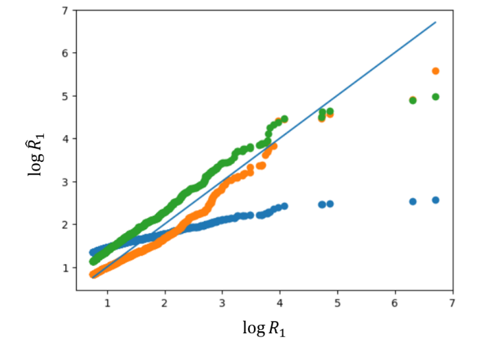
Figure 3: Log-QQ plot between the upper decile of 10000 radii samples from StdVAE (blue dots), ExtVAE_r (orange dots), UExtVAE_r (green dots) and the upper decile of the test data set of $R_{1}$. The log values of the true radius, denoted $\log R_{1}$ is on the x-axis, the log of the estimated radius, denoted $\log\hat{R}_{1}$, is on the y-axis. The dots should lie close to the blue line

In Table 1 and Figure 3, we study the ability of the benchmarked VAE schemes to sample heavy-tailed radius distribution. The results in Table 1 indicate that the evaluated cost remains roughly constant for our approaches when changing data sets, while it explodes for StdVAE. This indicates that our approaches, unlike StdVAE, successfully extrapolate the tail of the radius distribution. The log-QQ plots given in Figure 3 illustrate further that ExtVAE_r and UExtVAE_r schemes relevantly reproduce the linear tail pattern of the radius distribution while this is not the case for StdVAE. Figure 4 evaluates, for the compared methods, the evolution of the KL divergence between the true distribution and the simulated ones above a varying quantile $u$ (Equation 27). Again, the StdVAE poorly matches the target distribution with a clear increasing trend for quantiles $u$ such that $P(R_{1}>u)\geq 0.3$. Conversely, the KL divergence is much smaller and much more stable for ExtVAE_r and UExtVAE_r schemes, especially for large quantile values.

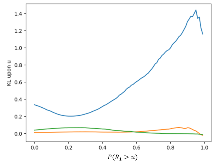
Figure 4: KL divergence between the radius distribution of the benchmared VAE models and the target heavy-tailed distribution: we display the KL divergence (see Equation 27) above quantile $u$ for $P(R_{1}>u)$ varying from $0$ to $1$ for StdVAE (blue curve), ExtVAE_r (orange curve) and UExtVAE_r. Numerically speaking, we sampled 10000 from each distribution and $u$ is taken as the quantile of the sampled reference data set.

Interestingly, for the different criteria, the results obtained with UExtVAE_r are very close or even indistinguishable from those obtained with ExtVAE_r. This suggests that the estimation of the tail index is accurate. In order to better assess the robustness of this estimation, we report the evolution of the tail index of UExtVAE_r as a function of the training epochs for randomly chosen initial values (Figure 5).

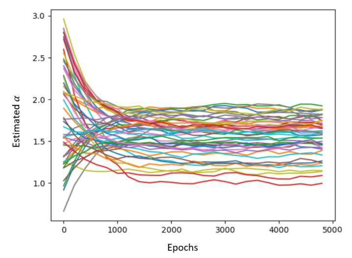
Figure 5: Evolution of the tail index $\alpha$ of UExtVAE_r during the training procedure: we report the value of the tail index as a function of the training epochs for training runs from different initial values. The initial values of $\alpha$ are sampled uniformly between $0.5$ to $3$. The true value of $\alpha$ is $1.5$.

Given the expected uncertainty in estimating the tail index (see Appendix D), UExtVAE_r estimates are globally consistent. We report meaningful estimation patterns since the reported curves tend to get closer to the true value as the number of epochs increase, although it might show some bias when initial value is far from the true tail index value. The mean value of the estimated tail index is $1.56$ with a standard deviation of $0.2$.
We now focus on the five-dimensional heavy-tailed case-study. The best parameterization for the likelihood of the conditional VAE is a Dirichlet parameterization (see Appendix C). An important advantage of our approach is the ability to generate samples on the simplex for a given radius as detailed in Section 4.3, and even to sample the angular measure. Figure 6 displays the angular measure projected onto the last two components of the simplex for the true angular measure, our ExtVAE approach and the ParetoGAN. For the latter, we approximate the angular measure by the empirical measure above a very high threshold. The ExtVAE shows a good agreement with the true distribution, though not as sharp. By contrast, the distribution sampled by the ParetoGAN tends to reduce to a single mode. The spatial direction of ParetoGAN extremes could therefore be erroneously interpreted as deterministic. This confirms the result of Proposition 8.

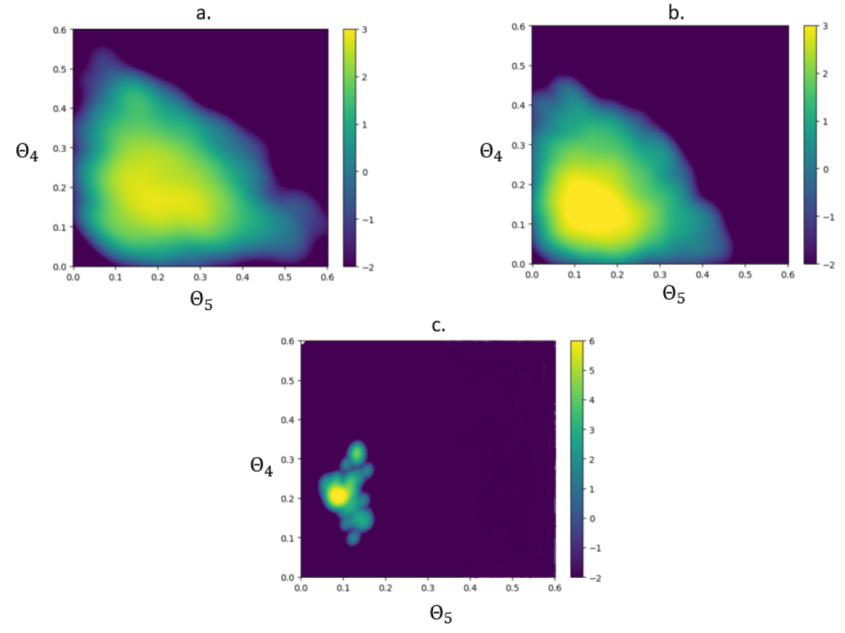
Figure 6: Log probability of the angular measure obtained with a. ExtVAE, b. true distribution, c. ParetoGAN, projected on axes 4 and 5 (named $\theta_{4}$ and $\theta_{5}$). For ParetoGAN, the estimation is based on 10000 samples at a high value of radius, typically above 10, which corresponds to the upper percentile of $R_{1}$ distribution.

Beyond the angular measure, we assess the sampling performance of the benchmarked schemes through an approximation of the Wasserstein distance (Equation 28) between 10000 generated items and the test set. The ExtVAE performs slightly better than the ParetoGAN (5.37 vs. 6.80). This is highlighted for high quantiles in Figure 7 where we plot the Wasserstein distance upon a radius threshold, dividing by the square of the threshold (see Equation 29), for ExtVAE and ParetoGAN. We focus on radius thresholds above 2, which corresponds to the highest decile. The ExtVAE performs again better than the ParetoGAN, especially for radius values between 2 and 4, corresponding roughly to quantiles between 0.90 and 0.95. We may recall that the ParetoGAN relies on the minimization of a Wasserstein metric, whereas the ExtVAE relies on a likelihood criterion. Therefore, we regard these results as an illustration of the better generalization performance of the ExtVAE, especially for the extremes.

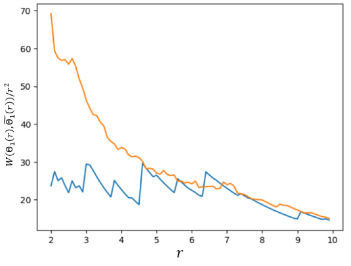
Figure 7: Wasserstein distance upon radius threshold $r$ divided by the square of $r$ calculated between 10000 samples drawn from generative approaches and test set. In orange, the generative method is the ParetoGAN and in blue it is our. The considered thresholds are above $2$, which is roughly the upper decile of the radii distribution.

At last, we estimate the threshold at which the radius and angle distributions can be considered as independent following the criterion proposed by Wan and Davis (2019). Although, by construction, there is no radius value from which there is a true independence, the estimator gives a radius above which one can approximately consider that some limit measure is reached. We compare in Figure 8 the p-values for assessing independence between the radius distribution and the angle distribution (see Appendix E.3). The p-values are represented as a function of the chosen threshold for each of the three considered data sets: the test data set, the data set sampled through the ExtVAE and the data set sampled through the ParetoGAN. The ExtVAE slightly underestimates the radius of the threshold compared to the true data ($1.3$ vs. $1.6$), while the ParetoGAN leads to a large overestimatation ($2.7$ vs. $1.6$). This illustrates further that the ExtVAE better captures the statistical features of high quantiles than ParetoGAN does. We regard the polar decomposition considered in the ExtVAE as the key property of the ExtVAE to better render the asymptotic distributions between the radius and the angle.

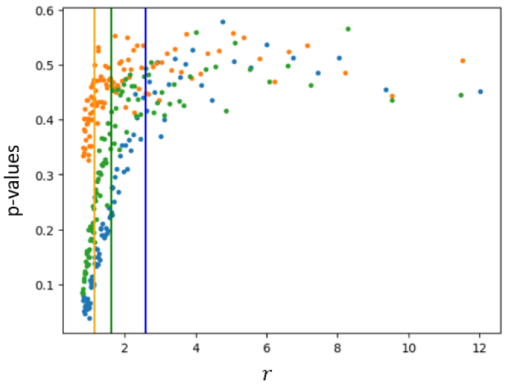
Figure 8: P-values for assessing independence between radius and angle distribution at different radius thresholds, computed according to Appendix E.3 for the test data set (green points), 10000 samples of the ExtVAE (orange points), and 10000 samples of the ParetoGAN (blue points). The vertical bars correspond to the threshold below which the p-values are less than $0.45$. Above this threshold, the radius and the angle can be roughly considered as independent. We refer to Wan and Davis (2019) for further details.

6.2 Danube River Discharge Case-study

Our second experiment addresses a real heavy-tailed multivariate data set. We consider the daily time series of river flow measurements over 50 years at five stations of the Danube river network (see Appendix A.2 for further details). River flow data are widely acknowledged to depict heavy-tailed distributions (see Katz et al., 2002). In reference to the numbering of the stations (see Figure 10), we note the random variables associated with the considered stations $X_{23},\ X_{24},\ X_{25},\ X_{26},\ X_{27}$. From the 50-year time series of daily measurements, we take a measurement every 25 days in the considered stations to form the training set. The remaining set constitutes the test set. There are 730 daily measurements in the training set, and 17486 daily measurements in the test set. We have deliberately chosen a training set size that is significantly smaller than the test set size. This allows us to stay within a distribution tail extrapolation problem while retaining sufficient test data to assess the relevance of our distribution tail estimate.
We focus on the question raised in introduction (see Figure 1): can we extrapolate and generate consistent samples in extreme areas not observed during the training phase? We focus on extreme areas of the form $\bigcap_{i=23}^{27}X_{i}>u_{i}$ with $u_{i}$ large predefined thresholds. This corresponds to flows exceeding predefined thresholds at several stations. Namely we define

$$A_{j}^{(p)}=\bigcap_{i=23}^{j}X_{i}>u_{i}^{(p)},$$ (23)

with $p$ a given probability level and $u_{i}^{(q)}$ the corresponding quantile of the flow $i$ in test set. The estimation of the probabilities of occurrence of such events is key to the assessment of major flooding risks along the river.
Our experiments proceed as follows. We train generative schemes on the training set as detailed in Section 4. For this case-study, the best parameterization for the likelihood of the angular part of the UExtVAE is a projection of a multivariate normal distribution (see Equation 4.3). As evaluation framework, we generate for each trained model a number of samples of the size of the test data set, and we compare the proportion of samples that satisfy a given extreme event to that in the test data set. We consider extreme events corresponding to quantile values of 0.9 and 0.99. Table 2 synthesizes this analysis for the StdVAE, UExtVAE and ParetoGAN. As illustrated, the training data set does not include extreme events for the 0.99 quantiles. Interestingly, the UExtVAE samples such extreme events with the same order of magnitude of occurrence as in the test data set. For instance, the proportion of samples that satisfy $A_{26}^{(0.99)}$ and $A_{27}^{(0.99)}$ is consistent with that observed in the test data set, respectively 0.2% and 0.18% against $0.4$% and $0.25$%. By contrast, the StdVAE cannot generalize beyond the training data set. The StdVAE truely generates events above 0.9 quantiles. However, it does not generate any element in $A_{26}^{(0.99)}$ and $A_{27}^{(0.99)}$.
ParetoGAN generates samples that satisfy $A_{25}^{(0.99)}$, $A_{26}^{(0.99)}$ and $A_{27}^{(0.99)}$. Although satisfactory, the sampled proportions are further from true proportions than for our approach. Moreover, by repeating the experiment, it seems that for $p\geq 0.9$, we always have $A_{25}^{(p)}=A_{26}^{(p)}$. This is probably due to the fact that the extremes are generated on a specific axis, as stated in Proposition 8.

Table 2: Evaluation of the generation of multivariate extremes for the Danube river data set: we report the proportion (in %) of elements satisfying $A_{j}^{(p)}$ (Equation 23) in the training and test data sets as well as data sets sampled from the trained StdVAE, UExtVAE and ParetoGAN with the same size as the test data set. We report this analysis for both $p=0.9$ and $p=0.99$.

	$p=0.9$
	Train	Test	UExtVAE	StdVAE	ParetoGAN
$A_{25}^{(p)}$	5.9	6.6	5.0	3.8	5.5
$A_{26}^{(p)}$	4.9	6.0	4.6	3.3	5.5
$A_{27}^{(p)}$	3.8	5.1	4.1	2.5	4.4

	q = 0.99
	Train	Test	UExtVAE	StdVAE	ParetoGAN
$A_{25}^{(p)}$	0.0	0.48	0.22	0.01	0.13
$A_{26}^{(p)}$	0.0	0.4	0.2	0.0	0.13
$A_{27}^{(p)}$	0.0	0.25	0.18	0.0	0.09

Note that the tail index of the radius of the discharge data set is not known a priori. Asadi et al. (2015) reports an estimate of $3.5\pm 0.5$ considering only the summer months. In our case, the tail index of the trained UExtVAE is of $4.5$. It is slightly higher than the value found by Asadi et al. (2015), which means a less heavy-tail distribution. Indeed, half of the annual maxima occurs in June, July or August, typically due to heavy summer rain events. Thus, we expect the summer months to depict heavier tails than the all-season data set, which is consistent with our experiments.

7 Conclusion

This study bridges VAE and EVT to address the generative modeling of multivariate extremes. Following the concept of multivariate regular variation, we propose a polar decomposition and combine a generative model of heavy-tailed radii with a generative model on the sphere conditionally to the radius. Doing so, we explicitly address the dependence between the variables at each radius, and in particular the angular measure. Experiments performed on synthetic and real data support the relevance of our approach compared with vanilla VAE schemes and GANs tailored for extremes. In particular, we illustrate the ability to consistently sample extreme regions that have been never observed during the training stage.
Our contribution naturally advocates for future work, especially for extensions to multivariate extremes in time and space-time processes (Basrak and Segers, 2009; Liu et al., 2012) as well as to VAE for conditional generation problems (Zheng et al., 2019; Grooms, 2021).

Acknowledgments and Disclosure of Funding

The authors acknowledge the support of the French Agence Nationale de la Recherche (ANR) under reference ANR-Melody (ANR-19-CE46-0011). Part of this work was supported by 80 PRIME CNRS-INSU, ANR-20-CE40-0025-01 (T-REX project), and the European H2020 XAIDA (Grant agreement ID: 101003469).

Appendix A Data Sets

This appendix provides details on the two data sets used in the experiments. One data set is synthetic (A.1) and the other is a true data set compiling flow measurements (A.2).

A.1 Synthesized Data Sets

We sample in a space of dimension $5$. We consider a sampling setting for the radius distribution denoted $R_{1}$ such that

$$R_{1}\sim\ 2{\bf U}\times{\bf Inv\Gamma}(\alpha_{1}=1.5\ ;\ \beta=0.6),$$

with $U$ uniform on $[0,1]$. From Breiman’s Lemma, the radius distribution is heavy-tailed with tail index $\alpha_{1}$.
The detailed expression of the conditional angular distribution ${\bf\Theta_{1}}\mid R_{1}=r$ is given by

$${\bf\Theta_{1}}\mid R_{1}=r\sim\mathbf{Diri}\left(\alpha_{1}(r),\alpha_{1}(r),\alpha_{2}(r),\alpha_{2}(r),\alpha_{2}(r)\right),$$ (24)

where $\alpha_{1}(r)=3\left(2-min(1,1/2r)\right)$, $\alpha_{2}(r)=3\left(1+min(1,1/2r)\right)$, and $Diri$ stands for Dirichlet distribution (see Appendix C).
Figure 9 gives the empirical pdf of $R_{1}$ based on 1000 samples.

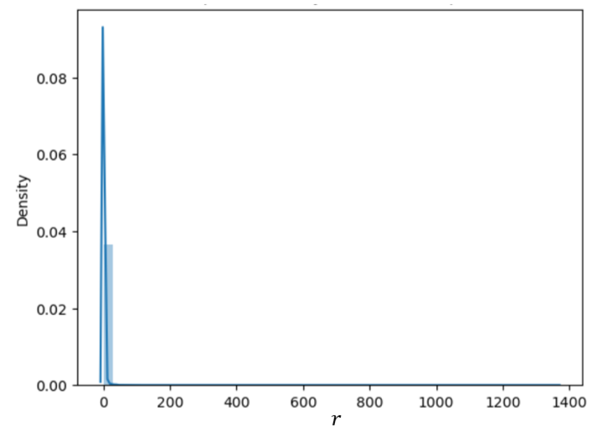
Figure 9: Empirical densities of synthesized radii $R_{1}$ based on 1000 samples.

A.2 Danube River Network Discharge Measurements

The upper Danube basin is an European river network which drainage basin covers a large part of Austria, Switzerland and of the south of Germany. Figure 10 shows the topography of the Danube basin as well as the locations of the 31 stations at which daily measurements of river discharge are available for a 50 years time window. Danube river network data set is available from the Bavarian Environmental Agency at http://www.gkd.bayern.de. As river discharges usually exhibit heavy-tailed distribution, this data set have been extensively studied in the community of multivariate extremes (see, e.g. Mhalla et al., 2020; Asadi et al., 2015). We consider measurements from a subset of $5$ stations (red triangles in Figure 10) from which we want to sample.

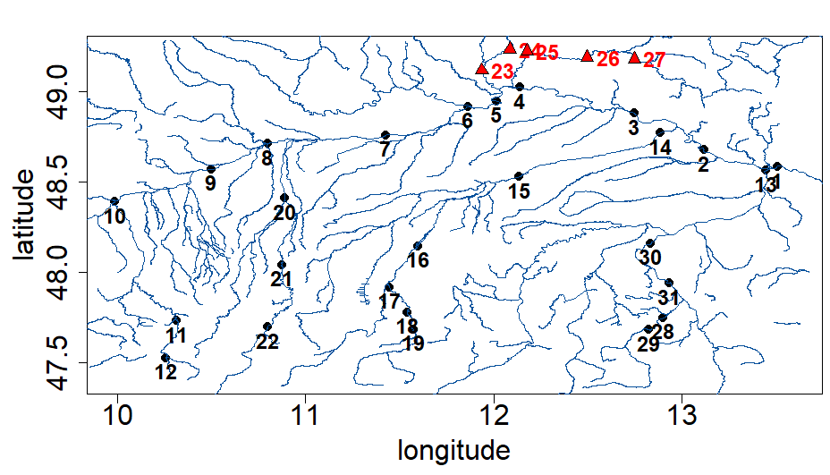
Figure 10: Topographic map of the upper Danube basin with 31 available gauging stations. A data set of 50 years of daily measurements is considered (from 1960 to 2010). our training set consists of all measurements for the 5 stations indicated by red triangles

Appendix B Additional Notions

We give in this appendix further explanations on some notions discussed in this article, and sometimes necessary for the development of the proofs (Appendix G).

B.1 Lipschitz Continuity

Definition 16

Let $\left(\mathbb{E},d_{\mathbb{E}}\right)$ and $\left(\mathbb{F},d_{\mathbb{F}}\right)$ be two metric spaces with $d_{\mathbb{E}}$ and $d_{\mathbb{F}}$ the respective metric on sets $\mathbb{E}$ and $\mathbb{F}$. A function $f:\mathbb{E}\rightarrow\mathbb{F}$ is called Lipschitz continuous if there exists a real constant $k\geqslant 0$ such that, for all $x_{1}$ and $x_{2}$ in $\mathbb{E}$,

$$d_{\mathbb{F}}\left(f\left(x_{1}\right),f\left(x_{2}\right)\right)\leqslant kd_{\mathbb{E}}\left(x_{1},x_{2}\right).$$ (25)

Remark 17

If $\mathbb{E}$ and $\mathbb{F}$ are normed vector spaces with respective norm $\|.\|_{\mathbb{E}}$ and $\|.\|_{\mathbb{F}}$, then $f$ Lipschitz continuous implies that there exists $k>0$ such that

$$d_{\mathbb{F}}\left(f(x),f\left({\bf 0}_{\mathbb{E}}\right)\right)\leqslant kd_{\mathbb{E}}\left(x,{\bf 0}_{\mathbb{E}}\right).$$

Consequently, $\|f(x)\|_{\mathbb{F}}\leqslant k\|x\|_{\mathbb{E}}+\|f({\bf 0}_{\mathbb{E}})\|_{\mathbb{F}}$.

B.2 Weak Convergence of Measures

Definition 18

Let $\mathbb{E}$ be a metric space and $\left(\mu_{n}\right)_{n\in\mathbb{N}}$ be a sequence of measures, then $\mu_{n}$ converges weakly to a measure $\mu$ as $n\to\infty$, if, for any $f:\mathbb{E}\longrightarrow\mathbb{R}$ real-valued bounded function,

$$\lim_{n\to\infty}\int_{\mathbb{E}}fd\mu_{n}=\int_{\mathbb{E}}fd\mu.$$

B.3 Equivalent definition of multivariate regular variation

The following definition of multivariate regularly varying vector is equivalent to Definition 4.

Definition 19

A random vector $\bf X$ has multivariate regular variation if there exists a function $b\to\infty$ and a Radon measure $\mu_{\bf X}$ called the limit measure such that

$$\lim_{t\to\infty}tP\left(\frac{\mathbf{X}}{b(t)}\in\bullet\right)\overset{v}{\longrightarrow}\mathbf{\mu_{X}}(\bullet).$$ (26)

Remark 20

The angular measure $\bf S_{X}$ defined in Equation (6) is related to the limit measure, for any measurable space of the simplex $\mathbb{A}$, and any measurable space $\mathbb{I}$ of $\mathbb{R}_{+}^{*}$, by

$$\mathbf{\mu_{X}}\circ T^{-1}(\mathbb{I},\mathbb{A})=\nu_{\alpha}(\mathbb{I})\times\bf S_{X}(\mathbb{A}),$$

where $T$ is the polar transform define for any vector $\bf x$ by $T({\bf x})=\left(\|{\bf x}\|\ ,\ \frac{{\bf x}}{\|{\bf x}\|}\right)$, and $\nu_{\alpha}$ a measure on $\mathbb{R}_{+}^{*}$ such that $\nu_{\alpha}([t,\infty])=ct^{-\alpha}$, with $c$ and $\alpha$ strictly positive constants.
The angular measure can be considered as the limit measure projected on the simplex.

Appendix C Dirichlet Parameterization of the Likelihood

We start by giving a definition of the Dirichlet distribution.

Definition 21

Let $(a_{i})_{i=1}^{m}$ be strictly positive constants and $m\geq 2$. A Dirichlet distribution with parameters $(a_{i})_{i=1}^{m}$ has a pdf defined by

$$f_{\bf Diri}({\bf x}\ ;\ (a_{i})_{i=1}^{m})=\frac{1}{B\left((a_{i})_{i=1}^{m}\right)}\prod_{i=1}^{m}x_{i}^{a_{i}-1},$$

$$\text{with }{\bf x}\in\mathbb{R}^{m}\text{ s.t }\sum_{i=1}^{m}x_{i}=1,$$

where $B$ is the multivariate beta distribution.

In particular, it means that the support of a Dirichlet distribution with parameters $(a_{i})_{i=1}^{m}$ is the $(m-1)$-dimensional simplex.
To use a Dirichlet parametrization of the likelihood, we change Equation (4.3) into

$$p_{\nu}({\bf s}\mid{\bf z}_{ang},r)\sim f_{\bf Diri}({\bf s}\ ;\ a_{\nu}({\bf z}_{ang},r)),$$

where $a_{\nu}$ outputs in $\left(\mathbb{R}^{+})\right)^{m}$.
Notice that Condition 14 must be modified, resulting in the following Condition.

Condition 22

$a_{\nu}$ is such that there exists a $z$-varying function $a_{\infty}$ which verifies for each ${\bf z}_{ang}$

$$\lim_{r\to+\infty}a_{\nu}({\bf z}_{ang},r)=a_{\infty}(\mathbf{z}_{ang}).$$

Again, $a_{\nu}({\bf z}_{ang},r)=h_{\nu}({\bf z}_{ang},\frac{1}{1+r})$, with $h_{\nu}$ Lipschitz continuous and $a_{\infty}(\mathbf{z}_{ang})=h_{\nu}({\bf z}_{ang},0)$. Similar to Remark 15, it is then simple to sample from the angular measure.

Appendix D Tail Index Estimation

Estimating the tail index of an univariate distribution from samples is not an easy task. To see this, we drew the Hill plot (see e.g Resnick, 2007, Section 4.4), (Xie, 2017, Section 2.2) for $R_{1}$ in Figure 11. The Hill plot is a common tool in the extreme value community for estimating the tail index of a distribution. If the graph is approximately constant from a certain order statistics, this constant is an estimator of the inverse of the tail index. We note that the Hill plot is of little use in this case because the graph does not exhibit clearly a plateau. Other methods are also broadly used to estimate the tail index within the extreme value community such as maximum likelihood estimation. It involves fitting a GP distribution (Equation 4) to the subset of data above a certain threshold (see Coles et al., 2001, for details). For example, on train data set of $R_{1}$, the maximum likelihood estimation gives an estimation of $1.28$ for the tail index when the threshold corresponds to a $0.8$-quantile while it becomes $1.67$ for a $0.9$-quantile.

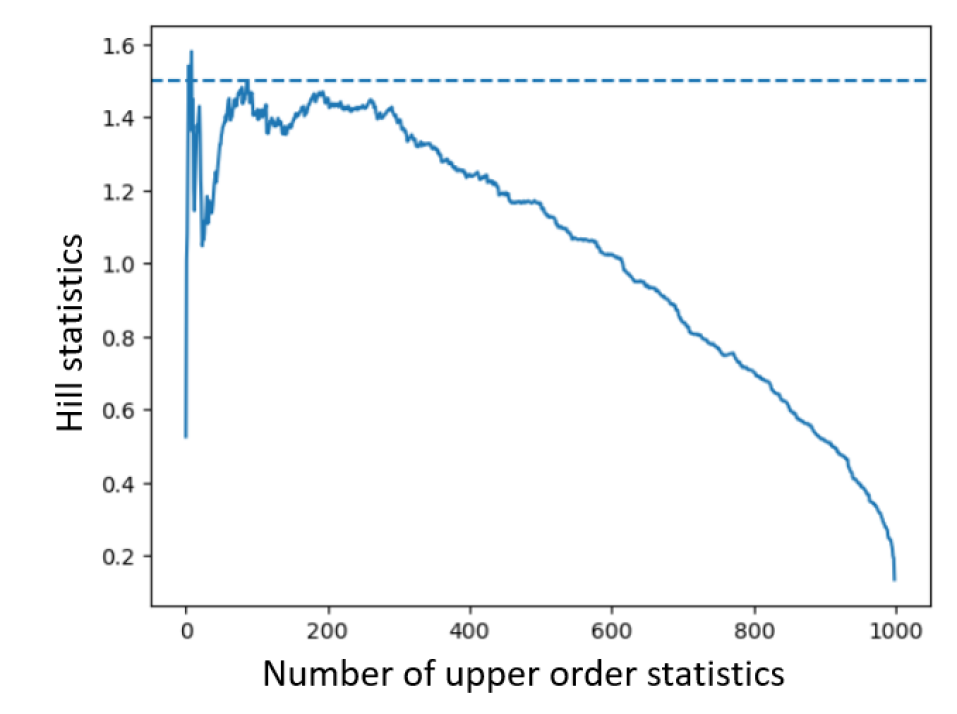
Figure 11: Hill plot for the 1000 $R_{1}$ samples of train and validation set (blue curve), the dashed line indicates the true value of the tail index, i.e. $1.5$.

Appendix E Criteria

In this section, we present detailed explanations of the different criteria we use to evaluate the approaches compared in the experiments (Section 6). They aim to compare the radius distributions (E.1), in particular for the tail, the overall distributions in the multivariate space (E.2), and to provide useful statistics on the angular distributions (E.3).

E.1 KL Divergence upon Threshold

Let us assume that we have $n$ samples ${\bf R_{true}}=(R_{true}^{1},R_{true}^{2},...,R_{true}^{n})$ from the true radius distribution and $m$ samples ${\bf R_{gen}}=(R_{gen}^{1},R_{gen}^{2},...,R_{gen}^{m})$ from a generative approach. Let denote $\tilde{\bar{F}}_{true}$, $\tilde{\bar{F}}_{gen}$ empirical estimators of the tail functions chosen to be non-zero above the upper observed value. Then the empirical estimate $\hat{K}_{u}({\bf R_{true}},{\bf R_{gen}})$ of the KL divergence beyond a threshold $u$ is given by

$$\hat{K}_{u}({\bf R_{true}},{\bf R_{gen}})= -1-\frac{1}{N_{n}}\sum_{i=1}^{m}\log\left(\frac{\tilde{\bar{F}}_{gen}(max(R_{gen}^{i},u))}{\tilde{\bar{F}}_{gen}(u)}\right)$$ (27)

$$-1-\frac{1}{M_{m}}\sum_{i=1}^{n}\log\left(\frac{\tilde{\bar{F}}_{true}(max(R_{true}^{i},u))}{\tilde{\bar{F}}_{true}(u)}\right),$$

where $N_{n}$ and $M_{m}$ are the number of samples above threshold $u$ respectively among ${\bf R_{true}}$ and ${\bf R_{gen}}$.

E.2 Wasserstein Distance

Assume we have $n$ samples ${\bf X}=({\bf x}_{1},{\bf x}_{2},...,{\bf x}_{n})$ from a random vector $X$ and $m$ samples ${\bf Y}=({\bf y}_{1},{\bf y}_{2},...,{\bf y}_{n})$ from another random vector with same dimension. Then, the Wasserstein distance we used is defined by

$$W({\bf X},{\bf Y})=\left(\min_{\gamma\in\mathbb{R}_{+}^{n\times m}}\sum_{i,j}\gamma_{i,j}\|{\bf x}_{i}-{\bf y}_{j}\|_{2}\right)^{\frac{1}{2}},$$ (28)

$$\mbox{with }n\gamma{\bf 1}={\bf 1}\ ;\ m\gamma^{T}{\bf 1}={\bf 1},$$

with ${\bf 1}$ a vector filled with ones, and $\|.\|_{2}$ the euclidean distance. The rescaled version of the Wasserstein distance beyond a threshold $r$ is then given by

$$W_{r}({\bf X},{\bf Y})=\frac{W({\bf X_{r}},{\bf Y_{r}})}{r^{2}},$$ (29)

where ${\bf X_{r}}$ (respectively ${\bf Y_{r}}$) consists of the elements of ${\bf X}$ (respectively ${\bf Y}$) of norm greater than $r$.

E.3 Threshold selection

Let us consider ${\bf X}$ a random vector of $\mathbb{R}^{d}$ with a polar decomposition $(R,{\bf\Theta})$. $({\bf X_{1}},{\bf X_{2}},\cdots,{\bf X_{N}})$ a sequence of observed vector of ${\bf X}$, with corresponding polar coordinates $R_{i}$ and ${\bf\Theta}_{i}$. Given a decreasing sequence of candidate radius threshold ${r_{k}}$, we want to find the smallest such as $R$ and ${\bf\Theta}$ can be considered independent. To assess independence between radius and angular distributions, Wan and Davis (2019) relies on the following hypothesis testing framework:

• $H_{0}$: $R/r_{k}$ and ${\bf\Theta}$ are independent given $R>r_{k}$,

• $H_{1}$: $R/r_{k}$ and ${\bf\Theta}$ are not independent given $R>r_{k}$.

Considering this, the authors propose a p-value for computing $H_{0}$ with respect to $H_{1}$, such that the p-value follows a uniform distribution if $H_{0}$ is true and is close to $0$ when $H_{1}$ is true. Thus, for a given threshold, when we average the p-values, we should find about $0.5$ if $H_{0}$ is true and closer to $0$ when $H_{1}$ is true.
To compute the p-values, the authors rely on the notion of empirical distance covariance (Székely et al., 2007).

Definition 23

The emprical covariance between $N$ observations $\{{\bf X_{i}}\}_{i=1}^{N}$ of a random vector ${\bf X}$ and $N$ observations $\{{\bf Y_{i}}\}_{i=1}^{N}$ of a random vector ${\bf Y}$ is given by

$$T_{N}({\bf X},{\bf Y}) =\frac{1}{N^{2}}\sum_{i,j=1}^{N}\|{\bf X_{i}}-{\bf X_{j}}\|_{2}\|{\bf Y_{i}}-{\bf Y_{j}}\|_{2}+\frac{1}{N^{4}}\sum_{i,j,k,l=1}^{N}\|{\bf X_{i}}-{\bf X_{j}}\|_{2}\|{\bf Y_{k}}-{\bf Y_{l}}\|_{2}$$

$$-\frac{2}{N^{3}}\sum_{i,j,k=1}^{N}\|{\bf X_{i}}-{\bf X_{j}}\|_{2}\|{\bf Y_{i}}-{\bf Y_{k}}\|_{2},$$

with $\|.\|_{2}$ the euclidean distance. Notice that ${\bf X}$ and ${\bf Y}$ have not necessarily equal sizes.

For a fixed threshold $r_{k}$, we consider the data sets

$$(R_{dep},{\bf\Theta}_{dep}) =\{(R_{i},{\bf\Theta}_{i}\ \text{ s.t. }R_{i}>r_{k}\},$$

$$R_{indep} =\{R_{i}\ \text{ s.t. }R_{i}>r_{k}\},$$

$${\bf\Theta}_{indep} =\{{\bf\Theta}_{i}\ \text{ s.t. }R_{i}>r_{k}\}.$$

We randomly choose a subsample of $(R_{dep},{\bf\Theta}_{dep})$ of size $n_{k}$ we denote $(R_{dep}^{n_{k}},{\bf\Theta}_{dep}^{n_{k}})$. We can then compute $T_{n_{k}}=T_{n_{k}}(R_{dep}^{n_{k}},{\bf\Theta}_{dep}^{n_{k}})$, which is the empirical covariance between the radii and angles within the subsample.
To compute a p-value of $T_{n,k}$ under the assumption that the conditional empirical distribution is a product of the conditional marginals, we take a large number $L$ of subsamples of size $n_{k}$ of $R_{indep}$ on the one hand, and of ${\bf\Theta}_{indep}$ on the other hand, respectively denoted $R_{indep}^{n_{k},l}$ and ${\bf\Theta}_{indep}^{n_{k},l}$ for $1\leq l\leq L$. We can compute the empirical covariances $\{\tilde{T}_{n,k}^{l}\}_{l=1}^{L}=T_{n_{k}}(R_{indep}^{n_{k},l},{\bf\Theta}_{indep}^{n_{k},l})$ between radii and angles.
The p-value $pv_{k}$ of $T_{n,k}$ is the empirical value of $T_{n,k}$ relative the $\{\tilde{T}_{n,k}^{l}\}_{l=1}^{L}$, i.e.

$$pv_{k}=\frac{1}{L}\sum_{i=1}^{L}\mathbf{1}_{\mathbb{R}^{+}}(T_{n_{k}}-\tilde{T}_{n,k}^{l}),$$

with $\mathbf{1}_{\mathbb{R}^{+}}$ the indicator function of the set of positive real numbers.
This process is repeated $m$ times, with different subsamples of $(R_{dep},{\bf\Theta}_{dep})$ leading to $m$ estimates of $pv_{k}$. The considered p-value is then the mean of these estimates. If the radius and angular distribution are independent, the p-value should be around $0.5$, otherwise it is closer to 0.

Appendix F Implicit Reparameterization

When it comes to optimization of the cost of Equation (2), explicit reparameterization (see Equation 3) is not feasible for the proposed framework introduced in Section 4.2. Leveraging the work of Figurnov et al. (2018), we use an implicit reparameterization. It consists in differentiating the Monte Carlo estimator of $E_{q_{\phi}(Z\mid r^{(i)})}[{f(Z)}]$ using

$$\nabla_{\phi}E_{q_{\phi}(Z\mid r^{(i)})}[{f(Z)}]=-E_{q_{\phi}(Z\mid r^{(i)})}[\nabla_{z}f(z)\nabla_{\phi}F_{q_{\phi}}(z)(\nabla_{z}F_{q_{\phi}}(z))^{-1}],$$

with $F_{q_{\phi}}$ the cumulative distribution function of $q_{\phi}$. An implicit reparameterization of Gamma distribution, as well as inverse Gamma and many others, is availalble as a Tensorflow package named TensorflowProbability.

Appendix G Proofs

G.1 Proof of Proposition 6

Proof  In a standard parameterization, we have

$$\bf{Z} \sim\mathcal{N}(\textbf{0},I_{n}),$$

$$X\mid[\bf{Z}=\bf{z}] \sim\mathcal{N}\left(\mu_{\theta}(\bf{z}),\sigma_{\theta}(\bf{z})^{2}\right),$$

according to Example 1.
The survival function of $X$ is

$$P(X>u) =\int_{\bf z}P(X>u\mid{\bf Z}={\bf z})p({\bf z})d{\bf z}$$

$$=\int_{\bf z}\frac{1}{(2\pi)^{\frac{n}{2}}}\left(\int_{u}^{+\infty}\frac{1}{\sqrt{2\sigma_{\theta}({\bf z})^{2}}}\exp\left(-\frac{\left(x-\mu_{\theta}({\bf z})\right)^{2}}{\sigma_{\theta}({\bf z})^{2}}\right)dx\right)\exp(-\bf{z}^{T}\bf{z})d\bf{z}$$

$$=\int_{\bf z}\frac{1}{(2\pi)^{\frac{n}{2}}}\operatorname{erfc}\left(\frac{u-\mu_{\theta}({\bf z})}{\sigma_{\theta}({\bf z})}\right)\exp(-\bf{z}^{T}\bf{z})d\bf{z},$$

where $\operatorname{erfc}$ is the complementary error function defined for $y\in\mathbb{R}$ by $\operatorname{erfc}(y)=1-\operatorname{erf}(y)$ with

$$\operatorname{erf}(y)=\frac{2}{\sqrt{\pi}}\int_{0}^{y}e^{-t^{2}}dt.$$

Let $\Omega(u)=\{{\bf z}\in\mathbb{R}^{n}\text{ s.t. }u-\mu_{\theta}(\bf{z})>0)$. We can write the survival function of $X$ this way:

$$P(X>u) =\int_{{\bf z}\in\Omega(u)}\frac{1}{(2\pi)^{\frac{n}{2}}}\operatorname{erfc}\left(\frac{u-\mu_{\theta}({\bf z})}{\sigma_{\theta}({\bf z})}\right)\exp(-\bf{z}^{T}\bf{z})d\bf{z}$$

$$+\int_{{\bf z}\in\overline{\Omega(u)}}\frac{1}{(2\pi)^{\frac{n}{2}}}\operatorname{erfc}\left(\frac{u-\mu_{\theta}({\bf z})}{\sigma_{\theta}({\bf z})}\right)\exp(-\bf{z}^{T}\bf{z})d\bf{z},$$

$$=f_{1}(u)+f_{2}(u).$$

We provide upper bounds for $f_{1}$ and $f_{2}$. Notice first that $f_{2}(u)\leq P({\bf z}\in\overline{\Omega(u)})$. As $\mu_{\theta}$ is Lipschitz continuous, there exists constants $k>0$ and $b\in\mathbb{R}$ such that $\mu_{\theta}(z)\leq k\|{\bf z}\|+b$ (see Remark 17).
It implies that, for $u>b$,

$$f_{2}(u) \leq P\left(\|{\bf z}\|\geq\frac{u-b}{k}\right)$$

$$\leq\frac{1}{2}\operatorname{erfc}\left(\frac{u-b}{k}\right)$$

$$\leq\exp\left(-\left(\frac{u-b}{k}\right)^{2}\right).$$ (30)

where we have used the inequality (Chiani et al., 2003)

$$\operatorname{erfc(y)}\leq e^{-y^{2}},\text{ for }y>0.$$ (31)

Equation (G.1) is the upper bound of $f_{2}$ we will use.
Concerning $f_{1}$, we use again inequality (31) to provide

$$f_{1}(u)\leqslant\int_{z\in\Omega(u)}\exp\left(-\left(\frac{u-\mu_{\theta}({\bf z})}{\sigma_{\theta}({\bf z})}\right)^{2}\right)p({\bf z})d{\bf z}.$$

As $\sigma_{\theta}$ is Lipschitz continuous, there exists constants $k^{\prime}>0$ and $b^{\prime}\in\mathbb{R}$ such that $\sigma_{\theta}({\bf z})\leq k^{\prime}\|{\bf z}\|+b^{\prime}$. Then, we can state that

$$f_{1}(u)\leqslant\int_{z\in\Omega(u)}\exp\left(-\left(\frac{u-\mu_{\theta}({\bf z})}{k^{\prime}\|{\bf z}\|+b^{\prime}}\right)^{2}\right)p({\bf z}).$$

For any $a>0$, we define the function

$$g_{u}({\bf z})=u^{a}\exp\left(-\left(\frac{u-\mu_{\theta}({\bf z})}{k^{\prime}\|{\bf z}\|+b}\right)^{2}\right).$$

The following holds:

$$\lim_{u\rightarrow+\infty}g_{u}({\bf z})=0.$$

Additionally, $g_{u}({\bf z})$ is maximal with respect to $u$ when $u=u^{*}({\bf z})$ with

$$u^{*}({\bf z})=\frac{\mu_{\theta}({\bf z})\pm\sqrt{\mu_{\theta}({\bf z})^{2}+2a\left(k^{\prime}\|{\bf z}\|+b^{\prime})^{2}\right)}}{2}.$$

Then, there exists $k^{\prime\prime}>0$ and $b^{\prime\prime}\in\mathbb{R}$ such that

$$\left|g_{u}({\bf z})p({\bf z})\right|\leqslant\left|u^{*}({\bf z})p({\bf z})\right|\leqslant\left(k^{\prime\prime}\|{\bf z}\|+b^{\prime\prime}\right)p({\bf z}).$$

By dominated convergence theorem, we can state that

$$\lim_{u\rightarrow+\infty}u^{a}f_{1}(u)=0.$$ (32)

From Equations (G.1) and (32), and consideration of Remark 2, we can conclude that $X$ is light-tailed.  

G.2 Proof of Proposition 8

Proof  In this proof we will extensively use the limit measure of multivariate regularly varying vector as defined in Definition 19. Remind from Remark 20 that the angular measure defined in Equation (6) is nothing else than the limit measure projected on the simplex. Consequently, proving that the angular measure is concentrated on some vectors of the simplex equates to prove that the limit measure is concentrated on some axes.
The proof proceeds by a series of step. First, we note that the prior $\bf Z$ has a limit measure located on the basis axes. Then, we prove that the limit measure of some transformations of a random vector with limit measure concentrated on some axes, have still limit measure concentrated on axes. The studied transformations are: multiplication by a matrix, addition of a bias, mapping with a ReLU unit. By applying iteratively this steps, we prove that $\bf X$ has a limit measure concentrated on axes, or equivalently an angular measure concentrated on vectors, for any ReLU neural network $f$. Additionally, it appears that the number of axes (or vectors) is less than the dimension $n$ of the input space.

First the limit measure $\mu_{\bf Z}$ of $\mathbf{Z}$ is concentrated on the basis axes. To be more explicit,

$$\mu_{\bf Z}\left(\mathbb{R}^{n}\backslash\cup_{i=1}^{n}\{te_{i},t>0\}\right)=0$$

with, for $i=1,\cdots,n$ $e_{i}=(0,\cdots,1,\cdots,0)$.
A proof is given in Resnick (2007), Section 6.5. This proof exploits the fact that the marginals of ${\bf Z}$ are i.i.d.

The following lemmas give, for some operations on a multivariate vector, the resulting transformation of its limit measure.

Lemma 24

If the d-dimensional random vector $\bf Y$ has multivariate regular variation with limit measure concentrated on some axes, and $\bf W$ is a $d\times n$ matrix, then $({\bf WY})_{+}$ has regular variation and its limit measure is concentrated on some axes.

Proof  In this proof, we define, for any Borel set $\mathbb{A}$, the inverse set in the non-negative orthant ${\bf W}^{-1}(\mathbb{A})=\{{\bf x}\in(\mathbb{R}^{+})^{n},\ {\bf Wx}\in\mathbb{A}\}$.

$$\lim_{t\to\infty}tP\left(\frac{(\mathbf{WY})_{+}}{b(t)}\in\bullet\right) =\lim_{t\to\infty}tP\left(\frac{\mathbf{Y}}{b(t)}\in\mathbf{W}^{-1}(\bullet)\right)$$

$$=\mathbf{\mu_{Y}}\circ\mathbf{W}^{-1}(\bullet)$$

$$=\mathbf{\mu_{WY}}(\bullet).$$

$({\bf WY})_{+}$ has regular variation.
Moreover if the limit measure of $\bf Y$ is concentrated on $n^{\prime}\leq n$ axes $\bigcup_{i=1}^{n^{\prime}}\{t\mathbf{v}_{i},\ t>0\}$, then for any measurable space $\mathbb{A}$,

$$\mathbf{\mu_{WY}}(\mathbb{A})\neq 0 \Longrightarrow\mathbf{\mu_{Y}}\circ\mathbf{W}^{-1}(\mathbb{A})\neq 0$$

$$\Longrightarrow\mathbf{W}^{-1}(\mathbb{A})\cap\left(\bigcup_{i=1}^{n^{\prime}}\{t\mathbf{v}_{i},\ t>0\}\right)\neq\emptyset$$

$$\Longrightarrow\mathbb{A}\cap\left(\bigcup_{i=1}^{n^{\prime}}\{t\mathbf{Wv}_{i},\ t>0\}\right)\neq\emptyset.$$

Consequently, the limit measure of $\bf WY$ is concentrated on $\bigcup_{i=1}^{n^{\prime}}\{t(\mathbf{W}\mathbf{v}_{i})_{+},\ t>0\}$. Notice that the limit measure of $\bf WY$ is then concentrated on a number of axes less or equal to $n^{\prime}$.

 

Lemma 25

If the d-dimensional random vector $\bf Y$ has multivariate regular variation with limit measure concentrated on axes, and $\bf b$ is a $m$-dimensional vector, then $(\mathbf{Y}+\mathbf{b})_{+}$ has multivariate regular variation and its limit measure is concentrated on axes.

Proof 

$$\lim_{t\to\infty}tP\left(\frac{(\mathbf{Y}+\mathbf{b})_{+}}{b(t)}\in\bullet\right)=\lim_{t\to\infty}tP\left(\frac{\mathbf{Y}}{b(t)}\in\bullet\right)\overset{v}{\longrightarrow}\mathbf{\mu_{Y}}(\bullet).$$

 
From Lemma 24 and Lemma 25 we get that for any random vector with multivariate regular variation and limit measure concentrated on some axes, any matrix $\bf W$ and bias $b$, $({\bf WY}+\mathbf{b})_{+}$ has multivariate regular variation with limit measure concentrated on some axes. This transformation corresponds to a layer of a ReLU neural network. Applying iteratively this transformation to the input random vector $\bf Z$, we obtain that $\mathbf{X}=f(\mathbf{Z})$ has multivariate regular variation with limit measure concentrated on axes, or equivalently angular measure concentrated on some vectors of the simplex. Additionally, the number of axes (or vectors) is less than $n$.  

G.3 Proof of Proposition 11

Proof  Let us consider $A$ an exponential distribution with scale parameter $c$ and $Z_{rad}$ an inverse-gamma distribution with parameters $(\alpha,\beta)$. The cumulative distribution function of $R$ is given by

$$P(R\leq t) =\int_{0}^{+\infty}P(A\leq z)\times\frac{t}{z^{2}}f_{\bf Inv\Gamma}\left(\frac{t}{z}\ ;\ \alpha,\beta\right)dz,$$

$$=1-\frac{\beta^{\alpha}}{t^{\alpha}\Gamma(\alpha)}\int_{0}^{+\infty}z^{\alpha-1}e^{-\frac{z}{c}}e^{-\frac{\beta z}{t}},$$

$$=1-\frac{\beta^{\alpha}}{t^{\alpha}}\left(\frac{1}{c}+\frac{\beta}{t}\right)^{-\alpha},$$

$$=1-\left(1+\frac{t}{\beta c}\right)^{-\alpha},$$

$$=1-\bar{H}_{\sigma,\xi}(t),$$

with $\sigma=\frac{\beta c}{\alpha}$ and $\xi=\frac{1}{\alpha}$. Consequently, $R$ follows a generalized Pareto distribution. Notice that we use the change of variable $u=z\left(\frac{1}{c}+\frac{\beta}{t}\right)$ from the second to the third line of the above equations.  

G.4 Proof of Proposition 13

Proof  Let $\alpha_{1}$, $\alpha_{2}$, $\beta_{1}$ and $\beta_{2}$ strictly positive constants. The following holds.

$$D_{KL}\left(f_{\bf Inv\Gamma}(z;\alpha_{1},\beta_{1})\mid\mid f_{\bf Inv\Gamma}(z;\alpha_{2},\beta_{2})\right) =E_{z\sim{\bf Inv\Gamma}(\alpha_{1},\beta_{1})}\left[\log\left(\frac{f_{\bf Inv\Gamma}(z;\alpha_{1},\beta_{1})}{f_{\bf Inv\Gamma}(z;\alpha_{2},\beta_{2})}\right)\right]$$

$$=E_{y\sim{\bf\Gamma}(\alpha_{1},\beta_{1})}\left[\log\left(\frac{f_{\bf Inv\Gamma}(\frac{1}{y};\alpha_{1},\beta_{1})}{f_{\bf Inv\Gamma}(\frac{1}{y};\alpha_{2},\beta_{2})}\right)\right]$$

$$=E_{y\sim{\bf\Gamma}(\alpha_{1},\beta_{1})}\left[\log\left(\frac{f_{\bf\Gamma}(y;\alpha_{1},\beta_{1})}{f_{\bf\Gamma}(y;\alpha_{2},\beta_{2})}\right)\right]$$

$$=D_{KL}\left(f_{\bf\Gamma}(z;\alpha_{1},\beta_{1})\mid\mid f_{\bf Inv\Gamma}(z;\alpha_{2},\beta_{2})\right).$$ (33)

Equation (13) holds from Equation (33) and the following result (Penny et al., 2006):

$$D_{KL}\left(f_{\bf\Gamma}(z;\alpha_{1},\beta_{1})\mid\mid f_{\bf\Gamma}(z;\alpha_{2},\beta_{2})\right)=(\alpha_{1}-\alpha_{2})\psi(\alpha_{1})-\log\frac{\Gamma(\alpha_{1})}{\Gamma(\alpha_{2})}$$

$$+\alpha\log\frac{\beta_{1}}{\beta_{2}}+\alpha_{1}\frac{\beta_{2}-\beta_{1}}{\beta_{1}}.$$

 

G.5 Proof of Proposition 12

Proof  The pdf of $R$ is given by

$$p(r) =\int_{0}^{+\infty}p_{\theta}(r\mid z_{rad})p_{\alpha}(z_{rad})dz_{rad},$$

$$=\int_{0}^{+\infty}f(r,z_{rad})dz_{rad},$$

with

$$f(r,z_{rad}) =f_{\mathbf{\Gamma}}\left(r\ ;\ \alpha_{\theta}(z_{rad}),\beta_{\theta}(z_{rad})\right)f_{\bf Inv\Gamma}(z_{rad}\ ;\ \alpha,1),$$

$$=\frac{r^{a_{\theta}-1}}{\Gamma(\alpha)\Gamma(a_{\theta})}z_{rad}^{-(\alpha+1)}\beta_{\theta}(z)^{a_{\theta}}e^{-r\beta_{\theta}(z)-\frac{1}{z}}.$$

From Equations (12) and (13), we can state the existence of $m$ and $M$ two strictly positive constants such that, for any $z$,

$$\frac{m}{z}\leq\beta_{\theta}(z)\leq\frac{M}{z}.$$

Consequently,

$$f_{1}(r,z_{rad})\leq f(r,z_{rad})\leq f_{2}(r,z_{rad})$$

with

$$f_{1}(r,z_{rad}) =\frac{r^{a_{\theta}-1}}{\Gamma(\alpha)\Gamma(a_{\theta})}z_{rad}^{-(a_{\theta}+\alpha+1)}m^{a_{\theta}}e^{-r\frac{M}{z_{rad}}-\frac{1}{z}},$$

$$f_{2}(r,z_{rad}) =\frac{r^{a_{\theta}-1}}{\Gamma(\alpha)\Gamma(a_{\theta})}z_{rad}^{-(a_{\theta}+\alpha+1)}M^{a_{\theta}}e^{-r\frac{m}{z_{rad}}-\frac{1}{z}}.$$

We can obtain analytical expressions of $\int_{0}^{+\infty}f_{1}(r,z_{rad})dz_{rad}$ and $\int_{0}^{+\infty}f_{2}(r,z_{rad})dz_{rad}$,

$$\int_{0}^{+\infty}f_{1}(r,z_{rad})dz_{rad} =\frac{r^{a_{\theta}-1}m^{a_{\theta}}}{\Gamma(\alpha)\Gamma(a_{\theta})}\int_{0}^{+\infty}z_{rad}^{-(a_{\theta}+\alpha+1)}e^{-r\frac{M}{z_{rad}}-\frac{1}{z_{rad}}}dz_{rad},$$

$$=\frac{r^{a_{\theta}-1}m^{a_{\theta}}}{\Gamma(\alpha)\Gamma(a_{\theta})}\Gamma(a_{\theta}+\alpha)(1+rM)^{-a_{\theta}-\alpha},$$

where we used the change of variables $u=\frac{1+rM}{z_{rad}}$. Using same arguments, we also obtain

$$\int_{0}^{+\infty}f_{2}(r,z_{rad})dz_{rad}=\frac{r^{a_{\theta}-1}M^{a_{\theta}}}{\Gamma(\alpha)\Gamma(a_{\theta})}\Gamma(a_{\theta}+\alpha)(1+rm)^{-a_{\theta}-\alpha}.$$

We have the asymptotic results when $r\to\infty$,

$$\int_{0}^{+\infty}f_{1}(r,z_{rad})dz_{rad}\propto r^{-\alpha-1},$$

$$\int_{0}^{+\infty}f_{2}(r,z_{rad})dz_{rad}\propto r^{-\alpha-1}.$$

Consequently, $r^{\alpha+1}p(r)$ is bounded away from $0$ when $r\to\infty$. Thus, ${r^{\alpha+1}P(R>r)}$ is also bounded away from $0$ when $r\to\infty$. The only possible value of the tail index of regular variation of the survival function of $R$ is $\alpha$.

References

- Allouche et al. (2022) Michaël Allouche, Stéphane Girard, and Emmanuel Gobet. Ev-gan: Simulation of extreme events with relu neural networks. Journal of Machine Learning Research, 23(150):1–39, 2022.
- Anderson and Meerschaert (1998) Paul L Anderson and Mark M Meerschaert. Modeling river flows with heavy tails. Water Resources Research, 34(9):2271–2280, 1998.
- Arjovsky et al. (2017) Martin Arjovsky, Soumith Chintala, and Léon Bottou. Wasserstein generative adversarial networks. In International conference on machine learning, pages 214–223. PMLR, 2017.
- Arora et al. (2016) Raman Arora, Amitabh Basu, Poorya Mianjy, and Anirbit Mukherjee. Understanding deep neural networks with rectified linear units. arXiv preprint arXiv:1611.01491, 2016.
- Asadi et al. (2015) Peiman Asadi, Anthony C Davison, and Sebastian Engelke. Extremes on river networks. The Annals of Applied Statistics, 9(4):2023–2050, 2015.
- Balkema and De Haan (1974) August A Balkema and Laurens De Haan. Residual life time at great age. The Annals of probability, 2(5):792–804, 1974.
- Basrak and Segers (2009) Bojan Basrak and Johan Segers. Regularly varying multivariate time series. Stochastic processes and their applications, 119(4):1055–1080, 2009.
- Bhatia et al. (2021) Siddharth Bhatia, Arjit Jain, and Bryan Hooi. Exgan: Adversarial generation of extreme samples. In Proceedings of the AAAI Conference on Artificial Intelligence, volume 35, pages 6750–6758, 2021.
- Bingham et al. (1989) Nicholas H Bingham, Charles M Goldie, Jozef L Teugels, and JL Teugels. Regular variation. Number 27. Cambridge university press, 1989.
- Boulaguiem et al. (2022) Younes Boulaguiem, Jakob Zscheischler, Edoardo Vignotto, Karin van der Wiel, and Sebastian Engelke. Modeling and simulating spatial extremes by combining extreme value theory with generative adversarial networks. Environmental Data Science, 1, 2022.
- Bradley and Taqqu (2003) Brendan O Bradley and Murad S Taqqu. Financial risk and heavy tails. In Handbook of heavy tailed distributions in finance, pages 35–103. Elsevier, 2003.
- Breiman (1965) Leonard Breiman. On some limit theorems similar to the arc-sin law. Theory of Probability & Its Applications, 10(2):323–331, 1965.
- Chavez-Demoulin and Roehrl (2004) Valérie Chavez-Demoulin and Armin Roehrl. Extreme value theory can save your neck. ETHZ publication, 2004.
- Chiani et al. (2003) Marco Chiani, Davide Dardari, and Marvin K Simon. New exponential bounds and approximations for the computation of error probability in fading channels. IEEE Transactions on Wireless Communications, 2(4):840–845, 2003.
- Clémençon et al. (2021) Stéphan Clémençon, Hamid Jalalzai, Stéphane Lhaut, Anne Sabourin, and Johan Segers. Concentration bounds for the empirical angular measure with statistical learning applications. arXiv preprint arXiv:2104.03966, 2021.
- Coles et al. (2001) Stuart Coles, Joanna Bawa, Lesley Trenner, and Pat Dorazio. An introduction to statistical modeling of extreme values, volume 208. Springer, 2001.
- Danielsson et al. (2016) Jon Danielsson, Lerby Murat Ergun, Laurens de Haan, and Casper G de Vries. Tail index estimation: Quantile driven threshold selection. Available at SSRN 2717478, 2016.
- Das et al. (2013) Bikramjit Das, Paul Embrechts, and Vicky Fasen. Four theorems and a financial crisis. International Journal of Approximate Reasoning, 54(6):701–716, 2013.
- De Haan and De Ronde (1998) Laurens De Haan and John De Ronde. Sea and wind: multivariate extremes at work. Extremes, 1:7–45, 1998.
- Drees and Sabourin (2021) Holger Drees and Anne Sabourin. Principal component analysis for multivariate extremes. Electronic Journal of Statistics, 15(1):908–943, 2021.
- Einmahl et al. (2013) John HJ Einmahl, Laurens de Haan, and Andrea Krajina. Estimating extreme bivariate quantile regions. Extremes, 16(2):121–145, 2013.
- Embrechts (2009) Paul Embrechts. Copulas: A personal view. Journal of Risk and Insurance, 76(3):639–650, 2009.
- Embrechts et al. (1999) Paul Embrechts, Sidney I Resnick, and Gennady Samorodnitsky. Extreme value theory as a risk management tool. North American Actuarial Journal, 3(2):30–41, 1999.
- Engelke and Ivanovs (2017) Sebastian Engelke and Jevgenijs Ivanovs. Robust bounds in multivariate extremes. 2017.
- Feder et al. (2020) Richard M Feder, Philippe Berger, and George Stein. Nonlinear 3d cosmic web simulation with heavy-tailed generative adversarial networks. Physical Review D, 102(10):103504, 2020.
- Figurnov et al. (2018) Mikhail Figurnov, Shakir Mohamed, and Andriy Mnih. Implicit reparameterization gradients. Advances in neural information processing systems, 31, 2018.
- Flamary et al. (2021) Rémi Flamary, Nicolas Courty, Alexandre Gramfort, Mokhtar Z Alaya, Aurélie Boisbunon, Stanislas Chambon, Laetitia Chapel, Adrien Corenflos, Kilian Fatras, Nemo Fournier, et al. Pot: Python optimal transport. J. Mach. Learn. Res., 22(78):1–8, 2021.
- Fortin and Clusel (2015) Jean-Yves Fortin and Maxime Clusel. Applications of extreme value statistics in physics. Journal of Physics A: Mathematical and Theoretical, 48(18):183001, 2015.
- Goodfellow et al. (2020) Ian Goodfellow, Jean Pouget-Abadie, Mehdi Mirza, Bing Xu, David Warde-Farley, Sherjil Ozair, Aaron Courville, and Yoshua Bengio. Generative adversarial networks. Communications of the ACM, 63(11):139–144, 2020.
- Grooms (2021) Ian Grooms. Analog ensemble data assimilation and a method for constructing analogs with variational autoencoders. Quarterly Journal of the Royal Meteorological Society, 147(734):139–149, 2021.
- Hernandez-Campos et al. (2004) Felix Hernandez-Campos, JS Marron, Gennady Samorodnitsky, and F Donelson Smith. Variable heavy tails in internet traffic. Performance Evaluation, 58(2-3):261–284, 2004.
- Huster et al. (2021) Todd Huster, Jeremy Cohen, Zinan Lin, Kevin Chan, Charles Kamhoua, Nandi O Leslie, Cho-Yu Jason Chiang, and Vyas Sekar. Pareto gan: Extending the representational power of gans to heavy-tailed distributions. In International Conference on Machine Learning, pages 4523–4532. PMLR, 2021.
- Jaini et al. (2020) Priyank Jaini, Ivan Kobyzev, Yaoliang Yu, and Marcus Brubaker. Tails of lipschitz triangular flows. In International Conference on Machine Learning, pages 4673–4681. PMLR, 2020.
- Jalalzai et al. (2018) Hamid Jalalzai, Stephan Clémençon, and Anne Sabourin. On binary classification in extreme regions. Advances in Neural Information Processing Systems, 31, 2018.
- Katz et al. (2002) Richard W Katz, Marc B Parlange, and Philippe Naveau. Statistics of extremes in hydrology. Advances in water resources, 25(8-12):1287–1304, 2002.
- Kingma and Ba (2014) Diederik P Kingma and Jimmy Ba. Adam: A method for stochastic optimization. arXiv preprint arXiv:1412.6980, 2014.
- Kingma and Welling (2013) Diederik P Kingma and Max Welling. Auto-encoding variational bayes. arXiv preprint arXiv:1312.6114, 2013.
- Laszkiewicz et al. (2022) Mike Laszkiewicz, Johannes Lederer, and Asja Fischer. Marginal tail-adaptive normalizing flows. In International Conference on Machine Learning, pages 12020–12048. PMLR, 2022.
- Liu et al. (2012) Yan Liu, Taha Bahadori, and Hongfei Li. Sparse-gev: Sparse latent space model for multivariate extreme value time serie modeling. arXiv preprint arXiv:1206.4685, 2012.
- Mhalla et al. (2020) Linda Mhalla, Valérie Chavez-Demoulin, and Debbie J Dupuis. Causal mechanism of extreme river discharges in the upper danube basin network. Journal of the Royal Statistical Society: Series C (Applied Statistics), 69(4):741–764, 2020.
- Nash et al. (2021) Charlie Nash, Jacob Menick, Sander Dieleman, and Peter W Battaglia. Generating images with sparse representations. arXiv preprint arXiv:2103.03841, 2021.
- Naveau et al. (2014) Philippe Naveau, Armelle Guillou, and Théo Rietsch. A non-parametric entropy-based approach to detect changes in climate extremes. Journal of the Royal Statistical Society: Series B (Statistical Methodology), 76(5):861–884, 2014.
- Pasche and Engelke (2022) Olivier C Pasche and Sebastian Engelke. Neural networks for extreme quantile regression with an application to forecasting of flood risk. arXiv preprint arXiv:2208.07590, 2022.
- Penny et al. (2006) W Penny, S Kiebel, and K Friston. Variational bayes. Elsevier, London, 2006.
- Pickands III (1975) James Pickands III. Statistical inference using extreme order statistics. the Annals of Statistics, pages 119–131, 1975.
- Razavi et al. (2019) Ali Razavi, Aaron Van den Oord, and Oriol Vinyals. Generating diverse high-fidelity images with vq-vae-2. Advances in neural information processing systems, 32, 2019.
- Resnick (2007) Sidney I Resnick. Heavy-tail phenomena: probabilistic and statistical modeling. Springer Science & Business Media, 2007.
- Rezende and Mohamed (2015) Danilo Rezende and Shakir Mohamed. Variational inference with normalizing flows. In International conference on machine learning, pages 1530–1538. PMLR, 2015.
- Rezende et al. (2014) Danilo Jimenez Rezende, Shakir Mohamed, and Daan Wierstra. Stochastic backpropagation and approximate inference in deep generative models. In International conference on machine learning, pages 1278–1286. PMLR, 2014.
- Rietsch et al. (2013) Théo Rietsch, P Naveau, N Gilardi, and Armelle Guillou. Network design for heavy rainfall analysis. Journal of Geophysical Research: Atmospheres, 118(23):13–075, 2013.
- Rootzén and Tajvidi (2006) Holger Rootzén and Nader Tajvidi. Multivariate generalized pareto distributions. Bernoulli, 12(5):917–930, 2006.
- Rudd et al. (2017) Ethan M Rudd, Lalit P Jain, Walter J Scheirer, and Terrance E Boult. The extreme value machine. IEEE transactions on pattern analysis and machine intelligence, 40(3):762–768, 2017.
- Székely et al. (2007) Gábor J Székely, Maria L Rizzo, and Nail K Bakirov. Measuring and testing dependence by correlation of distances. The annals of statistics, 35(6):2769–2794, 2007.
- Tencaliec et al. (2019) P. Tencaliec, A.-C. Favre, P. Naveau, C. Prieur, and G. Nicolet. Flexible semiparametric generalized Pareto modeling of the entire range of rainfall amount. Environmetrics, 31(2):e2582, 2019.
- Wan and Davis (2019) Phyllis Wan and Richard A Davis. Threshold selection for multivariate heavy-tailed data. Extremes, 22(1):131–166, 2019.
- Xie (2017) Xiaolei Xie. Analysis of Heavy-Tailed Time Series. PhD thesis, University of Copenhagen, Faculty of Science, Department of Mathematical …, 2017.
- Zhao et al. (2017) Tiancheng Zhao, Ran Zhao, and Maxine Eskenazi. Learning discourse-level diversity for neural dialog models using conditional variational autoencoders. arXiv preprint arXiv:1703.10960, 2017.
- Zheng et al. (2019) Chuanxia Zheng, Tat-Jen Cham, and Jianfei Cai. Pluralistic image completion. In Proceedings of the IEEE/CVF Conference on Computer Vision and Pattern Recognition, pages 1438–1447, 2019.