Résumé

We consider the problem of model building for rare events prediction in longitudinal follow-up studies. In this paper, we compare several resampling methods to improve standard regression models on a real life example. We evaluate the effect of the sampling rate on the predictive performances of the models. To evaluate the predictive performance of a longitudinal model, we consider a validation technique that takes into account time and corresponds to the actual use in real life.

Keywords : Rare events, longitudinal follow-up, oversampling, undersampling, SMOTE, ensemble-based methods, logistic regression.

1 Introduction

Prediction models for rare events appears in many research fields such as economic (Burez and Van den Poel,, 2008), politics (King and Zeng,, 2002), fraud detection (Bolton and Hand,, 2002) or bank regulation (Calabrese and Osmetti,, 2015). Modeling and predicting binary rare events present several difficulties. Strong imbalance between event and non-events induce biased estimations and poor predictive performances, usually underestimating the probability of event occurrences. In recent years, several strategies have been proposed to improve misclassification. For example, King and Zeng, (2002) propose an explanatory logistic regression model with bias correction in a case-control study. Calabrese and Osmetti, (2013) have developed a new regression model based on extreme value theory. More recently, Nuñez et al., (2017) improve the learning function in SVM by a low-cost post-processing strategy.

Another way to the improve predictive performance of a model with rare events is to rebalance artificially the dataset by resampling methods. For example, oversampling methods creates artificially new observations in the minority class, whereas undersampling methods delete observations in the majority class. Hybrid methods combine both oversampling and undersampling methods.

The choice of resampling rate, that is the final ratio between events and non-events, is a crucial point to improve predictive performance of the model. It is known that the optimal rate is highly dependent on the dataset (Batista et al.,, 2004; Zhu et al.,, 2017). Futhermore, resampling methods induce additional randomness in the dataset. The most common way to reduce this extra-variablity is to use aggregation methods (Breiman,, 1996). Other strategies to improve classifiers with rare events have been considered, such as weighting training instances (Pazzani et al.,, 1994) or using different misclassification costs for minority and majority events (Spears and Perlis,, 1989).

The aim of the paper is to compare several resampling and aggregation methods on a real-life longitudinal follow-up study. We discuss the way to evaluate predictive performance in the case of longitudinal studies and then choose the optimal sampling rate adapted to our data set.

In Section 2, we review resampling and ensemble based methods. We also discuss the way to evaluate the predictive performance adapted to longitudinal follow-up. In Section 3, we compare several strategies applied to a real life example: we have followed a soccer teams during one year and we aimed to evaluate the risk of muscle injury before each match. We discuss the crucial choice of the sampling rate and the effect of aggregation methods. We also show that SMOTE methods (Chawla et al.,, 2002) applied to our dataset performs poorly.

2 Prediction models and sampling methods

In this section, we present several resampling methods combined with aggregation to improve the predictive performance of a logistic regression.

2.1 Standard logistic regression

Here, we recall the bases of logistic regression. For an individual $i$ $(i=1,...,n)$, let $x_{i}$ be the $k+1$-vector of the $k$ explanatory variables plus the constant and let $y_{i}\in\{0,1\}$ be the binary response which follows a Bernoulli distribution with parameter $\pi_{i}=P(y_{i}=1\mid x_{i})$. In the standard logistic regression, it is assumed that

$$\pi_{i}=\frac{1}{1+e^{-x_{i}^{\prime}\beta}}$$ (1)

where $x^{\prime}$ is the transpose of $x$ and $\beta^{\prime}=(\beta_{0},\beta_{1},...,\beta_{k})$ is the vector of unknown parameters, usually estimated by maximum likelihood (see e.g. McCullagh and Nelder, (1989)). The asymptotic variance of $\widehat{\beta}$ is

$$V(\hat{\boldsymbol{\beta}})=\left[\sum_{i=1}^{n}\pi_{i}\left(1-\pi_{i}\right)\mathbf{x}_{i}\mathbf{x}_{i}^{\prime}\right]^{-1}$$ (2)

For a new individual $x$, the probability of the event $y=1$ is predicted by

$$\widehat{\pi}(x)=\frac{1}{1+e^{-x^{\prime}_{i}\widehat{\beta}}}=\widehat{\mathbb{P}}(y=1\mid x)$$

When the dataset contains few events, say less than 5%, it is known that logistic regression underestimate the probability of events and then poor predictive performances (see (King and Zeng,, 2002))

2.2 Balancing unbalanced dataset

To overcome drawbacks induced by the unbalanced datasets, several sampling methods can be used to artificially rebalance the dataset. Several resampling methods on real data are compared in Batuwita and Palade, (2010); Batista et al., (2004); Liu et al., (2009); Zhu et al., (2017). Drummond and Holte, (2003) show that oversampling is better than undersampling and Japkowicz, (2000) that random oversampling or undersampling methods improve substantially the predictive performance of the models so that more sophisticated oversampling or down-sizing methods approaches appear unnecessary. All these studies show that the best resampling method is highly dependent on the dataset.

In this section, we review the most common sampling methods, which can be used alone or combined.

2.2.1 Undersampling methods

The first way to rebalance an unbalanced dataset is to reduce the number of observations in the majority class (non-events). A random undersampling with rate $r$, $0<r<1$, creates a new dataset by removing at random from the initial dataset a proportion $r$ of observations from the majority class. If $r=0$, then all the observations of the majority class are kept. If $r=0.7$, then $70\%$ of the observations of the majority class are removed.

In the case of very rare events, King and Zeng, (2002) propose to used case-control designs (see also Breslow,, 1996). This strategy is equivalent to selecting randomly one non-event for every event, resulting in a completely balanced dataset. In that case, if the proportion of events is $p$, then the rate of the undersampling is $r=(1-2p)/(1-p)$. Another more sophisticated strategy has been proposed in Tomek, (1976): for each event, the idea is to remove a non-event that form a Tomek link. Kubat, (2000) considers situations where Tomek link methods does not guarantee a performance gain.

The main drawback of undersampling methods is the loss of information when the number of removed observations is large. In Section 2.3, we consider aggregated methods that limit this loss of information.

2.2.2 Oversampling methods

At the opposite of undersampling methods, oversampling methods increase artificially the number of observations in the minority class (events). A random oversampling with rate $(a\!:\!b)$ creates new observations by duplicating at random observations in the minority class until there are $a$ non-events for $b$ events in the new dataset. An oversampling $(1\!:\!1)$ results in a completely balanced dataset. An oversampling $(2\!:\!1)$ results in a dataset with 2 non-events for 1 event.

SMOTE (Chawla et al.,, 2002) is a more sophisticated method that creates synthetic observations in the minority class as follows: for each event observation, choose at random one of the $k$ nearest neighbors that belongs to the minority class, with $k$ fixed. The new synthetic observation is chosen at random between these two observations. It is also possible to reiterate the process to increase the oversampling rate. Figure 1 shows the effect of SMOTE with $k=2$ and with one synthetic observation generated by events.

2.2.3 Hybrid sampling

It is known that these methods have some cons. Random undersampling can discard potentially useful data, whereas random oversampling creates exact copies of existing instances that may induce overfitting. To overcome these features, a solution is to mix undersampling and oversampling methods. For example, a random undersampling method with rate $c$ combined with a $(a\!:\!b)$-oversampling method consists in removing at random a proportion $c$ of non-event and then perform an oversampling to obtain $a$ non-events for $b$ events.

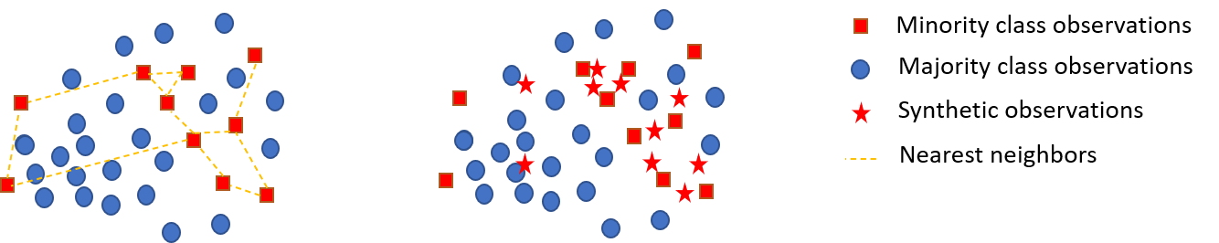
Figure 1: SMOTE: for each event, one synthetic observation is created from one of the two nearest neighbors at random.

As a remark, random over/under sampling methods can be seen as weighted logistic regressions (Manski and Lerman,, 1977) where the weights are random. For the resampled dataset, the log-likelihood of the logistic regression can be written:

$$\ln L_{w}(\boldsymbol{\beta}|\mathbf{y}) =\sum_{i\,/\,y_{i}=1}w_{i}\ln\left(\pi_{i}\right)+\sum_{i\,/\,y_{i}=0}w_{i}\ln\left(1-\pi_{i}\right)$$

where the weight $w_{i}$ is the number of replication of $x_{i}$ for $y_{i}=1$ in the random oversampling process and $w_{i}=0/1$ for $y_{i}=0$ in the random undersampling process.

2.3 Ensemble-based methods

Each sampling method described above induces a supplementary part of randomness in the dataset and therefore more variability in the predictions. Ensemble-based methods are the most common way to reduce this variability. The idea is to create $K$ datasets from the same resampling scheme and to aggregate the predictors. Therefore, for a new individual $i$ with covariate $x_{i}$, the predicted probability of event $\widehat{\pi}_{i}$ is given by

$$\widehat{\pi}_{i}=\frac{1}{K}\sum_{k=1}^{K}\widehat{\pi}_{i}^{[k]},$$

where $\widehat{\pi}_{i}^{[k]}$ is the predictor obtained from the k^th dataset. The choice of $K$ will be discussed in Section 3.2.3.

As a variant, when using a pure oversampling methods, the non-events may be replaced by $K$ bootstrap samples, similarly to Bagging (Breiman,, 1996). In the same way, when using a pure oversampling method, the events may be replaced by a bootstrap sample of them. The effects of this bootstrap variant on the aggregated predictors are displayed in Table 2.

2.4 Predictive performance evaluation in longitudinal follow-up

To evaluate the predictive performance of a model, training and test datasets should be chosen carefully. In longitudinal follow-up studies, events are highly dependent on the past and change the future. In this context, it is impossible to use standard validation strategies like cross validation or random split of the dataset into learning and test datasets. Indeed, with this strategy, the risk is to confuse causes and consequences and to overestimate predictive performances. Therefore, it is more natural to use a longitudinal strategy (see Fig. 2) that corresponds to the way the models are used in real life: at time $t$, we only use previous information to predict the risk $\widehat{\pi}_{ti}$ to have an event on the individual $i$, then we compare our prediction with the real observation $y_{ti}$. At the end, we have a collection of $(\hat{\pi}_{tj},y_{tj})$, $t=1,...,T$ and $i=1,...,I$.

The usual way to compare the ability of several models to predict a binary response is to compare their ROC curves, AUCs or Peirce indices. We recall that a ROC curve is a parametric curve defined as follows: for a given threshold $0\leq\gamma\leq 1$, we predict $y_{ti}$ by $\hat{y}_{ti}=0$ if $\widehat{\pi}_{ti}<\gamma$ and $\hat{y}_{ti}=1$ if $\widehat{\pi}_{ti}\geq\gamma$. Then, we compare the predicted response $\hat{y}_{ti}$ with the real outcome $y_{ti}$. The sensitivity and the specificity, which depend on $\gamma$ are defined by

$$\textrm{sensitivity}(\gamma)=\dfrac{TP}{TP+FN}\quad\quad\textrm{specificity}(\gamma)=\dfrac{TN}{TN+FN}$$

with $TN$, $TP$, $FN$, $FP$ are the number of true negative, true positive, false negative, false positive. For example $TP=\#\{y_{ti}=1\;,\;\hat{y}_{ti}=1\}$. The ROC curve is therefore the parametric curve $\{(\mathop{\textrm{sensitivity}}(\gamma),1-\mathop{\textrm{specificity}}(\gamma))\;;\;0\leq\gamma\leq 1\}$. As shown in Raeder et al., (2012), the choice of an evaluation metric plays an important role in learning on unbalanced data. From the ROC curve, we can derived two global metrics: the area under ROC curve (AUC) and the Pierce index (PI) defined by

$$\textrm{PI}=\max_{\gamma\in[0,1]}\{\textrm{sensitivity}(\gamma)+\textrm{specificity}(\gamma)-1\}.$$

which is particularly adapted to rare events.

The Pearce index represents a good compromise between sensitivity and specificity. It can be shown that $\textrm{PI}=1-d^{*}$, where $d^{*}$ is the Manhattan distance between the point (0,1) and its closest point on the ROC curve. It is also the euclidean distance between the further point on the ROC curve from the diagonal, up to a factor $\sqrt{2}$. The model with the highest AUC or PI will be considered as the best predictive model.

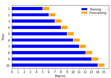
Figure 2: Longitudinal validation.

3 Comparison of resampling methods in a real life longitudinal follow-up.

In this section, we apply and compare the methods described in Section 2 in a real life situation. We have followed a soccer teams of the french Ligue 1 Championship during the season 2018-2019. We aim to build a model that evaluate the individual risk of non-contact muscle injury for each player before each match. To build the model, we use the data collected during the seasons 2015-2018 and the season 2018 until the match. A review of football player injury prediction methods can be found in Eetvelde et al., (2021). Several predictive methods are compared in Carey DL et al., (2018). From Daniel and Javier, (2017), the average incidence of muscle injuries for a player during a match is about 4%. In our dataset we observe a similar rate, so that non-contact muscle injuries are considered as rare events.

To evaluate the predictive performances of the model, we use the longitudinal validation described in Section 2.4. Before each match, we predict the risk of muscle injury for each player $i$ based on all preceding observations. Then, we and compare the prediction with the real outcomes, that is, muscle injury or not of player $i$ during the match. Of course, players that do not play the match are not considered.

During the season, 50 matches had been played and 16 non-contact muscle injuries have been observed. To train the model before the first match, we use the data collected during the seasons 2015-2018. Then, iteratively, we use the data collected until the day before each match of the season 2018-2019 to predict the probability of injury for the next match.

3.1 The dataset

The dataset include 42 soccer players on which data are collected daily and during matches. After each match, the response variable is observed : $y=1$ if an injury is observed and $y=0$ otherwise. For each player, we have the following covariates that are considered in the literature as risk factors.

• Cumulative workload during training and matches over 21 days.

• Cumulative playing time over 21 days.

• Recovery time: number of days since the last match.

• Risk of relapse: ratio between the number of days disability due to injury and the average number of days of disability in the team. It aims to quantify the risk of relapse after an injury.

• Acceleration ratio: ratio between the number of accelerations performed over the 7 days preceding the match and the number of accelerations performed on the 21 days preceding the match

• Deceleration ratio: ratio between the number of deceleration performed over the 7 days preceding the match and the number of deceleration performed on the 21 days preceding the match

• Speed ratio: ratio between the average speed over the 7 days preceding the match and the average speed over the 21 days preceding the match.

• Player ID: player identifier.

Workload, Cumulative playing time and Recovery time allow to quantify player activity. Acceleration, deceleration and speed ratio are used to assess the player sport performance before the match. Another important covariate is the player ID. In usual longitudinal studies, the aim is to extrapolate the model on other individuals. Therefore individuals (here, players) are considered as random effects. In our case, we want to predict future observations on the individuals that are included in the studies. Therefore, players are considered as fixed effect, allowing to personalize the risk of injury. We will not consider interaction between factors, since they have not shown, in preliminary studies, any improvement of the predictive ability of the models, mainly due to overfitting.

3.2 Comparison of resampling methods

In this section, we compare the predicitive performance of several resampling strategies applied to logistic regression. The performances metrics are evaluated on the 50 matches played during the season 2018-2019, by using the longitudinal validation described in Section 2.4. Several resampling methods are evaluated: undersampling alone, undersampling + bootstrap on events, oversampling alone, oversampling + bootstrap on the events, both oversampling and undersampling. When several sampling strategies are combined, we first use undersampling, then oversampling or SMOTE.

3.2.1 Effect of sampling rates on predictive performances

Here, we evaluate the effect of the balancing rate on AUC in random oversampling, SMOTE and random undersampling methods applied to logistic regression. The results are displayed in Fig. 3. Each method is run 15 times. Then, we compute the average AUC over the runs. We also compute the standard deviation for both metric. Note that the initial dataset imbalance is $(25\!:\!1)$, that is 25 non-events for 1 event.

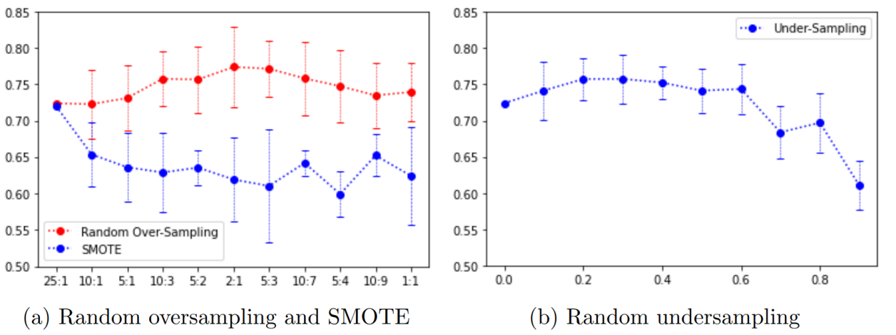
Figure 3: Average AUC over 15 runs with twice the standard deviation against sampling rates.

For random oversampling (Fig. 3.a, red line), the average AUC increases from $0.72$ to $0.77$ when the sampling rate goes from $(25\!:\!1)$ to or $(5\!:\!3)$. Then, the AUC decreases, probably due to an overfit on the events. For SMOTE (Fig. 3.a, blue line) the effect on AUC is always negative. This is mainly due to events that are isolated in the covariate space and therefore create synthetic events in the middle of non-events: for example, in Fig. 1 two isolated events on the left induce two synthetic events in the middle of a cluster of non-events.

In Fig. 3.b, we can see that undersampling methods slightly improve the average AUC for an undersampling rate between 0.2 and 0.3 with a AUC gain about 0.03. When the sampling rate is too large, say greater than 0.7 for our dataset, the predictive performance of the model worsen since too many non-event individuals are removed.

3.2.2 Comparison of several pure and hybrid resampling methods

Table 1: Comparison of average AUC and Peirce index with standard deviation (std) for several resampling methods.

Here, we compare random oversampling and undersampling methods studied in Section 3.2.1 with hybrid methods, SMOTE or plain logistic regression. Again, for each strategy, we run 15 times the model. So, we obtain an average AUC and Peirce index with related standard deviations. Sensitivities and specificities are calculated for the run whose Peirce index is the closest to the average. The results are displayed in Table 1 and for some models, ROC curves are displayed in Fig. 4.

The plain logistic regression, i.e. without additional resampling method, has an AUC equal to 0.72 and a Peirce index equal to 0.510 with a sensitivity $0.75$ and a specificity $0.76$. Random oversampling improves the prediction performance for a large range of sampling rates. For example, an oversampling rate of $(5\!:\!3)$ gives average AUC and Peirce equal to $0.78$ and $0.56$, the sensibility increases to $0.75$ whereas the specificity slightly decreases from to $0.75$. As already seen in Section 3.2.1, SMOTE methods give poor results and undersampling should be used with caution, only with a small removal rate.

In conclusion, for our dataset, the resampling methods with highest AUC and Peirce index are pure random oversampling $(5\!:\!3)$ followed by hybrid undersampling $0.3$ / oversampling $(5\!:\!3)$. Note that the second method has a slightly lower average Peirce index (0.547) for the same average AUC.

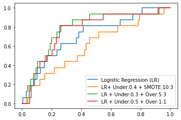
Figure 4: Comparison of ROC curves for several resampling methods with aggregation.

3.2.3 Ensemble-based methods

Resampling methods add randomness in the output. Ensemble based methods, described in section 2.3, aim to stabilize the model and in some situations to improve the predictive performance, similarly to Bagging methods. There is no consensus about the right number of aggregations, which is usually between 20 and 100 for Bagging methods (Breiman,, 1996; Bühlmann and Yu,, 2002), depending on the dataset.

To evaluate the effect of the number of aggregations needed to stabilize the prediction for our dataset, we display, in Fig. 5, AUC and Peirce index against to the number of aggregations for two of the best models obtained in Section 3.2.2: the first one is an hybrid undersampling with $r=0.3$ and overampling $(5\!:\!3)$ and the second one is an undersampling with $r=0.5$ combined with a bootstrap sampling on the events. For the two models, AUC is stabilized after 20 iterations (Fig. 5.a and 5.b) whereas Peirce index needs more iterations to be stabilized (Fig. 5.c and 5.d) .

To save computer time, we now compare ensemble-based methods with 20 iterations for the models used in Section 3.2.2. The results are displayed in Table 2, line 1-6, whose means and standard deviations of AUC and Peirce index, sensitivity and specificity are obtained in the same way as in Table 1. We omit SMOTE methods that have shown poor results.

It can be observed that the main effect of aggregation methods is to reduce the variability of AUC and Peirce index. For example, for random undersampling with rate $0.3$, the standard deviation of AUC decreases from 0.063 to $0.005$. For random oversampling $(5\!:\!3)$ it decreases from $0.007$ to $0.002$. The effects of aggregation methods on the mean AUC and Peirce index depend on the resampling methods. For undersampling, aggregation methods improve slightly the average AUC and Peirce index, whereas there is no significant effect for oversampling.

In table 2, line 8-11, we have considered a bootstrap of the events when an undersampling method is used and a bootstrap sample of the non-events when an oversampling methods is used. It is seen that Bootstrap has no significant effect on the mean AUC and Peirce index, but increases their variability. In line 7 of the same table, we have performed a stratified bootstrap on the events and non-events. The predictive performance is better than that of the plain logistic regression but lower than over/under sampling or hybrid methods with optimized rate.

Among all the models considered here, the best predictive models are the hybrid models undersampling 0.5 and oversampling $(1\!:\!1)$ or undersampling 0.3 and oversampling $(5\!:\!3)$.

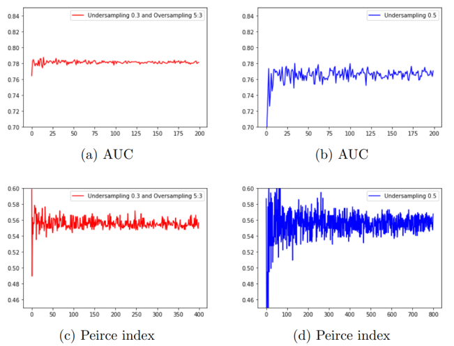
Figure 5: AUC and Peirce index variation against the number of aggregation in ensemble-based methods for two resampling methods.

Table 2: Effect of the ensemble-based methods on the mean and standard deviation of AUC and Peirce index for several resampling methods.

3.2.4 Longitudinal validation vs cross-validation

Longitudinal validation described in Section 2.4 corresponds to the way the model is used in practice. It is therefore the most relevant method to evaluate the predictive performance.

Usual cross-validation methods such as leave-one-out cross-validation (LOOCV) use future information to predict the outcome. For example, for our data set analyzed with plain logistic regression, i.e. without resampling methods, AUC and Peirce indices obtained by LOOCV are equal to 0.84 and 0.665 whereas they are equal to 0.72 and 0.51 for longitudinal validation. For the best strategy found in 3.3.2, i.e. 0.5 undersampling followed by oversampling (5:3) with aggregation, AUC and Peirce index are equal to 0.85 and 0.672 for LOOCV and to 0.78 and 0.566 for longitudinal validation. So, we can see that LOOCV overestimate the true predictive performance of the models.

Another validation strategy consists in using the dataset based on the seasons 2015-2018 to train the model and the dataset of the season 2018-2019 to test the model (see, e.g., Carey DL et al.,, 2018). This approach is relevant if it is not possible to update the model with fresh data or if we want to use the model for other individuals or players. However, in the case of individual follow-up, the model loose information from the near past. For example, with this validation approach, AUC and Peirce index are equal to 0.650 and 0.25 for the plain logistic regression 0.681 and 0.31 for the hybrid undersampling 0.5, oversampling $(5\!:\!3)$. We can see that this validation strategy tends to underestimate the predictive performance of the model as it is used in practice.

4 Conclusion

We have shown how resampling methods can improve subtantially predictive models for rare events. The best resampling method and the optimal sampling rate are specific to each dataset. Most often they are calibrated by cross validation. However, in the case of longitudinal follow-up, usual cross-validation methods tend to overestimate the predictive quality of the model. Therefore, it is important to use a validation method adapted to longitudinal follow-up.

Pure random oversampling or hybrid under/oversampling with optimized sampling rate appear to be the most effective method to improve a logistic regression for rare events. SMOTE was ineffective for our dataset structure, mainly due to isolated events in the space of explanatory variables. Moreover, ensemble-based methods and predictor aggregation reduce the effects of the variability of resampling methods onto the predictors.

Acknowledgment

The authors are grateful to Olivier Brachet (Innovation Performance Analytics) for having provided the dataset.

Funding

This research has been supported by the European Regional Development Fund and the Region Auvergne-Rhone-Alpes