Exploring quasiprobability approach to quantum work in the presence of initial coherence: Advantages of the Margenau-Hill distribution

Abstract

In quantum thermodynamics, the two-projective-measurement (TPM) scheme provides a successful description of stochastic work only in the absence of initial quantum coherence. Extending the quantum work distribution to quasiprobability is a general approach to characterize work fluctuation in the presence of initial coherence. However, among a large number of different definitions, there is no consensus on the most appropriate work quasiprobability. In this article, we list several physically reasonable requirements including the first law of thermodynamics, time-reversal symmetry, positivity of second-order moment, and a support condition for the work distribution. We prove that the only definition that satisfies all these requirements is the Margenau-Hill (MH) quasiprobability of work. In this sense, the MH quasiprobability of work shows its advantages over other definitions. As an illustration, we calculate the MH work distribution of a breathing harmonic oscillator with initial squeezed states and show the convergence to classical work distribution in the classical limit.

I Introduction

In stochastic thermodynamics, the studies of thermodynamics were extended from the ensemble average level to the stochastic trajectory level [1, 2], where work and other thermodynamic concepts are identified as stochastic quantities [3]. These stochastic quantities were found to satisfy some interesting and strong relations known as fluctuation theorems [4]. On even more microscopic scales, quantum effects play a crucial role in thermodynamic phenomena [5, 6, 7, 8, 9, 10, 11, 12]. Due to the absence of the concept of trajectory in quantum mechanics, it is a necessary but challenging task to define the quantum stochastic work [13]. After some early efforts on the operator-of-work scheme [14, 15], the stochastic work defined by the two-projective-measurement (TPM) scheme [16, 17] is now the standard way provided no quantum coherence in the initial state. Based on this definition, the fluctuation theorems are readily recovered when the quantum system is driven from canonical equilibrium. The TPM scheme is also widely used to define other quantum thermodynamic quantities, including heat and particle number exchange [18]. The consequent quantum thermodynamic theory has flourished in both theoretical and experimental aspects [5, 6, 7, 8, 9, 10, 11, 12, 19, 20].

However, the TPM scheme fails to characterize the quantum stochastic work when the initial state of the system contains quantum coherence, that is, the initial density matrix does not commute with the initial Hamiltonian. The first measurement process becomes invasive and destroys the coherence of the initial state [21, 22]. Quantum coherence indeed brings some advantages in quantum thermodynamics. It has been shown that quantum coherence can improve the performance of quantum heat engines [23, 24, 25, 26, 27, 28, 29, 30], and can be used to enhance the work extraction [31, 32]. To characterize the fluctuation with initial coherence, a generalized definition of stochastic work is needed, which should recover the standard result based on the TPM scheme if there is no initial coherence. Unfortunately, the no-go theorem for quantum work prohibits a genuine probability framework to reconcile the first law and the reproduction of the TPM result [33]. A possible resolution is to adopt the quasiprobability for the work distribution, which allows the distribution to take negative or complex values. It is found that the work quasiprobability is a direct signature of quantum contextuality [34].

Quasiprobability distributions arise naturally in the study of quantum mechanics when treating noncommutative observables [35, 36, 37, 38]. Recently, there is growing interest in studying quasiprobability of work in quantum thermodynamic phenomena [39, 40]. So far, there have been several different proposals on the definitions of quantum work. For example, the Kirkwood-Dirac (KD) quasiprobability of quantum work [41, 42, 43] and the Margenau-Hill (MH) quasiprobability of work [44] are based on famous quasiprobability distributions [38, 36], which are widely used in quantum optics. The Full-Counting (FC) quasiprobability of work [45] is another kind of quasiprobability, which is related to full counting statistics [46]. Most recently, a class of quasiprobability distributions that generalizes the MH and FC ones was proposed [47]. A natural question arises: which definition of quantum work quasiprobability is the most appropriate one?

In this article, we propose several requirements for quantum work and further show that only the MH quasiprobability of work meets all these requirements. Hence, it is the most appropriate definition of quantum stochastic work. This paper is organized as follows. In Sec. II, we first briefly review the TPM scheme and the no-go theorem for quantum work. In Sec. III, we list the requirements for an appropriate quantum work and discuss their physical implications. Among these requirements, the support condition is the most conspicuous one. In Sec. IV, we prove the only definition that satisfies all the requirements is the MH quasiprobability of work. In Sec. V, a comparison of some definitions is discussed from the perspective of these requirements. In Sec. VI, we calculate the MH work quasiprobability for a breathing quantum harmonic oscillator starting from a squeezed state and show the quantum-classical correspondence principle for MH work distribution.

II A review of no-go theorem for quantum work

The isolated driving process is one of the basic processes in the study of nonequilibrium statistical mechanics. Let us consider a nonequilibrium quantum driving process governed by the Schrödinger equation during the time interval $[0,\tau]$. The time-dependent Hamiltonian is $H_{S}(t),0\leq t\leq\tau$, and the initial density matrix for the system is denoted as $\rho$. Here we use the subscript $S$ in the Hamiltonian to denote the Schrödinger picture. For simplicity, we set the reduced Planck constant $\hbar=1$ except in Sec. VI. The time evolution of the system is characterized by the time-evolution operator $U(\tau)=\mathcal{T}\exp(-\mathrm{i}\int_{0}^{\tau}\mathrm{d}tH_{S}(t))$, where $\mathcal{T}$ is the time-ordering operator. In the Heisenberg picture, the Hamiltonian operator is $H_{H}(t)=U(t)^{-1}H_{S}(t)U(t)$ while the quantum state remains invariant. In the later discussion, we will mostly work in the Heisenberg picture and adopt several shorthand notations: $H_{0}=H_{H}(0)$, $H_{1}=H_{H}(\tau)$, $U=U(\tau)$. We diagonalize the initial and final Hamiltonians in the Heisenberg picture as $H_{0}=\sum_{n}\epsilon_{n}^{0}\Pi_{n}^{0}$ and $H_{1}=\sum_{n}\epsilon_{n}^{1}\Pi_{n}^{1}$, where $\Pi_{n}^{0},\Pi_{n}^{1}$ are projective operators corresponding to eigenvalues $\epsilon_{n}^{0},\epsilon_{n}^{1}$.

Under the stochastic description, work performed in this process is a random variable, denoted by $W$. The corresponding probability distribution function is $P(w)$, which is related to the probability by $\Pr(a<W\leq b)=\int_{a}^{b}P(w)\mathrm{d}w$. If the initial state does not contain quantum coherence, that is, $[\rho,H_{0}]=0$, the standard two-projective measurement (TPM) gives the following quantum work probability distribution:

$$P_{\mathrm{TPM}}(w) =\sum_{ij}p_{ji}p_{i}\delta(w-(\epsilon_{j}^{1}-\epsilon_{i}^{0}))$$ (1)

$$=\sum_{ij}\Tr[\Pi_{j}^{1}\Pi_{i}^{0}\rho\Pi_{i}^{0}\Pi_{j}^{1}]\delta(w-(\epsilon_{j}^{1}-\epsilon_{i}^{0})).$$

The above expression has a clear physical meaning. $p_{i}=\Tr[\Pi_{i}^{0}\rho\Pi_{i}^{0}]$ is the probability of the $i$-th energy level when measuring the initial Hamiltonian. Supposing $\tilde{\rho}_{i}=\Pi_{i}^{0}\rho\Pi_{i}^{0}/\Tr[\Pi_{i}^{0}\rho\Pi_{i}^{0}]$ is the collapsed state after the first measurement, $p_{ji}=\Tr[\Pi_{j}^{1}\tilde{\rho}_{i}\Pi_{j}^{1}]$ is the transition probability from the $i$-th initial energy level to the $j$-th final energy level while doing the second measurement after the time evolution. Since the system is isolated, the work is identified as the energy difference $\epsilon_{j}^{1}-\epsilon_{i}^{0}$ between two measurements with the associated probability $p_{ji}p_{i}$ of this realization.

For the states without initial coherence, the first measurement does not perturb the overall quantum state. In this case, the TPM work distribution is consistent with the first law of thermodynamics as well as work fluctuation theorems. However, in the presence of initial quantum coherence, the first measurement destroys the initial state, and the off-diagonal terms of the density matrix in the energy basis are eliminated. Due to its invasive nature, the TPM scheme for quantum work fails to describe a process with initial coherence. As a direct consequence, the average work defined by the TPM scheme is in contradiction with the first law of thermodynamics. Despite the success of quantum thermodynamics based on the TPM scheme, its validity is restricted to only a small portion of initial states.

Furthermore, a famous no-go theorem shows that under a genuine probability framework, there is no way to generalize the TPM scheme to incorporate initial coherence [33]. In Ref. [33], a genuine probability distribution implies the following three constraints on $P(w)$. The first two constraints come from the axioms of probability theory and are easy to understand: $P(w)\geq 0$, and $\int_{-\infty}^{+\infty}P(w)\mathrm{d}w=1$. The third constraint is a property regarding the initial state known as convexity: For any $0\leq\lambda\leq 1$, the distribution satisfies $P(w;\lambda\rho_{1}+(1-\lambda)\rho_{2})=\lambda P(w;\rho_{1})+(1-\lambda)P(w;\rho_{2})$. An explanation of convexity is given in the next section. The no-go theorem for quantum work [33] states that the following two requirements cannot be simultaneously fulfilled under the above genuine probability framework. One is the first law of thermodynamics for the average work, $\expectationvalue{W}=\Tr[(H_{1}-H_{0})\rho]$. The other is the reduction to the standard TPM result for initial states without coherence. These two requirements are both very important in quantum thermodynamics but contradict each other.

III requirements for quasiprobability of quantum work

The quasiprobability approach abandons the positivity assumption of the probability distribution function to resolve the contradiction. In the quasiprobability framework, the distribution function $P(w)$ could take negative or even complex values. Other two constraints, namely, the normalization relation and the convexity still hold. We summarize here the modified conditions for a quasiprobability distribution.

• Distribution function is complex-valued (or real-valued) and normalized

  $$P(w)\in\mathbb{C},$$ (2)

  $$\int P(w)\mathrm{d}w=1.$$

• The distribution function exhibits convexity with respect to the initial density operator: For any $0\leq\lambda\leq 1$,

  $$P(w;\lambda\rho_{1}+(1-\lambda)\rho_{2})=\lambda P(w;\rho_{1})+(1-\lambda)P(w;\rho_{2}).$$ (3)

This convexity condition originates from the nature of the classical probability because the mixed density matrix $\lambda\rho_{1}+(1-\lambda)\rho_{2}$ is equivalent to randomly choosing the initial state from $\rho_{1}$ and $\rho_{2}$ with (classical) probability $\lambda$ and $1-\lambda$ respectively, and the result for $\lambda\rho_{1}+(1-\lambda)\rho_{2}$ should be a direct combination of two independent parts.

Since the average work in quantum mechanics is well-defined and has been widely used for a long time before the concept of stochastic work, there is no doubt that the first law of thermodynamics at the ensemble average level should be a criterion.

• The first law of thermodynamics for average work

  $$\int wP(w)\mathrm{d}w=\Tr\left[(H_{1}-H_{0})\rho\right].$$ (4)

Physically, the first law requires the average work to be the average of the energy change.

Another condition that appears in the formulation of no-go theorem for quantum work is the reproduction of TPM scheme, which requires the quantum work to match the standard definition by TPM scheme in the case when the initial state contains no quantum coherence. The achievements of quantum thermodynamics such as the quantum fluctuation theorems based on the TPM scheme serve as a justification. Nevertheless, this requirement is not directly used in the later proof but appears as a consequence of other requirements. We regard it as an extra condition which is labeled as requirement (E1) in this paper.

• Reproduction of TPM scheme:

  $$P(w)=P_{\mathrm{TPM}}(w),\quad\text{if }\commutator{\rho}{H_{0}}=0.$$ (5)

Before listing other requirements, it is meaningful to introduce the consequences of the above requirements. The convexity shows the distribution exhibits a linear dependence on the initial state, and we assert that $P(w)$ can be expressed as

$$P(w)=\Tr[M(w)\rho],$$ (6)

where $M(w)$ is a bounded operator irrelevant to $\rho$. This expression is intuitively valid because the right-hand side also keeps the linear property on $\rho$. Strict proof is given in Appendix A based on functional analysis.

As illustrations, we summarize the expressions of $M(w)$ in some typical definitions for quantum work. From Eq. (1), $M(w)$ for the TPM work distribution is

$$M_{\mathrm{TPM}}(w)=\sum_{ij}\Pi_{i}^{0}\Pi_{j}^{1}\Pi_{i}^{0}\delta(w-(\epsilon^{1}_{j}-\epsilon^{0}_{i})).$$ (7)

A $q$-class of quasiprobability distributions proposed in Refs. [47, 48] generalizes the MH work quasiprobability distribution and FC work quasiprobability distribution. $M(w)$ for $q$-class is

$$M_{q}(w)=\sum_{ijk}\frac{1}{2}\left[\Pi_{k}^{0}\Pi_{j}^{1}\Pi_{i}^{0}+\Pi_{i}^{0}\Pi_{j}^{1}\Pi_{k}^{0}\right]$$ (8)

$$\times\delta(w-[\epsilon_{j}^{1}-q\epsilon_{i}^{0}-(1-q)\epsilon_{k}^{0}]),$$

with a parameter $0\leq q\leq 1/2$. The cases with $q=0$ and $q=1/2$ reduce to the MH and FC work quasiprobability distributions respectively.

For initial states without coherence, $\commutator{\rho}{\Pi^{0}_{n}}=0$, all the above distribution functions coincide with each other. On the other hand, we can easily verify the first law for the quasiprobability in $q$-class. Thus, in contrast to the no-go theorem, as we abandon the positivity of probability, we arrive at a multiple-choice result: there are many work quasiprobability distributions that satisfy both the first law (W2) and the reproduction of the TPM scheme (E1).

In addition to the above conditions (W0)-(W2) and (E1), from physical consideration, we list several other requirements. They are later used to demonstrate the validity of the MH quasiprobability of work.

The following requirement plays the core role in this paper, which roots in our physical understanding of the concept of work.

• Support condition: The distribution function $P(w)$ is solely determined by $H_{0}$, $H_{1}$, and $\rho$. If $P(w)\neq 0$, then there exists $i,j$ such that $w=\epsilon^{1}_{j}-\epsilon_{i}^{0}$. And if $k\neq i,l\neq j$ for all possible $i,j$, then $P(w)$ does not depend on $\epsilon^{0}_{k},\Pi^{0}_{k}$ and $\epsilon^{1}_{l},\Pi^{1}_{l}$.

Here is an explanation of this requirement. As is shown in most proposals, the quantum work is viewed as a quantity related to the initial and final Hamiltonians in the Heisenberg picture, $H_{0}$ and $H_{1}$, with no regard to the evolution details during the process. We adopt this as an assumption for an isolated quantum process; work only depends on $H_{0}$, $H_{1}$, and the initial state $\rho$. The distribution function can be explicitly written as $P(w;H_{1},H_{0},\rho)$. Furthermore, inspired by the physical meaning of the TPM scheme, we assume that the stochastic work characterizes the energy level transition. Since the energy is distributed only at the eigenvalues, the support (nonzero points) of $P(w)$ is restricted to the differences between the final and initial energy eigenvalues. That is, $P(w)\neq 0$ implies $w$ can be expressed as $\epsilon_{j}^{1}-\epsilon_{i}^{0}$. Also, we expect that the transition probability between two energy levels has nothing to do with other energy levels. In consideration of possible degeneracy of the energy difference, let us suppose $w$ belongs to the support of $P(w)$, and $(i_{1},j_{1}),(i_{2},j_{2}),\dots$ are all the pairs such that $w=\epsilon_{j_{m}}^{1}-\epsilon_{i_{m}}^{0}$. If $k\neq i_{m}$ for any $m$, then $P(w)$ has nothing to do with the $k$-th initial energy level, and $P(w)$ does not depend on $\epsilon_{k}$ and $\Pi^{0}_{k}$. This is also true for the $l$-th final energy level if $l\neq j_{m}$ for any $m$. This accounts for the last sentence in (W3).

In this paper, we do not directly require the reproduction of the TPM scheme (E1) but try to extract the physical implication behind the TPM scheme and introduce the support condition (W3). As we will see, the reproduction of the TPM scheme will emerge as a consequence of other requirements.

Furthermore, there should be a linear relation between work and Hamiltonian, which was explicitly proposed in Ref. [48]. Let us consider a global rescaling transform of the time-dependent Hamiltonian, $H_{H}^{\prime}(t)=\lambda H_{H}(t)$. While $\rho$ is fixed, we expect $W^{\prime}$ in this rescaled protocol to exhibit the same distribution as $\lambda W$. In another transform, the Hamiltonian is shifted by a c-number (classical number) $H_{H}^{\prime}(t)=H_{H}(t)+e(t)$, which corresponds to different choices of the zero point of the energy. In this case, we naturally expect $W^{\prime}$ to exhibit the same distribution as $W+e(\tau)-e(0)$. Combining these two kinds of transforms, we have the following requirement.

• A linear rescaling condition on the Hamiltonian: Under the rescaling transform $H_{H}(t)\rightarrow\lambda H_{H}(t)+e(t)$ with fixed initial state, the work rescales as $W\rightarrow W^{\prime}\overset{d}{=}\lambda W+e(t)-e(0)$. Here, $\overset{d}{=}$ means both sides have the same distribution.

The zeroth-order moment and the first-order moment are fixed by the normalization relation and the first law, respectively. Besides, in stochastic thermodynamics, the amplitude of fluctuation can be quantified by the variance, which should be always non-negative. Equivalently, the second-order moment is also non-negative. We adopt this as a requirement of work distribution for arbitrary initial states.

• Positivity of the second-order moment:

  $$\expectationvalue{W^{2}}=\int w^{2}P(w)\mathrm{d}w\geq 0.$$ (9)

The time-reversal symmetry is the last requirement for $P(w)$, which was proposed in Ref. [49]. In the standard formulation, the time-reversed process of an original process is implemented as follows. The anti-unitary time-reversal operator $\Theta$ is involved, and we will use an overline to denote quantities in the time-reversed process. In the Schrödinger picture, the initial state is set to be the time-reversed final state in the original process $\bar{\rho}(0)=\Theta\rho(\tau)\Theta^{-1}$. The time-reversed Hamiltonian is also equipped with the time-reversal operator, and the time parameter in the Hamiltonian evolves backward: $\bar{H}_{S}(t)=\Theta H_{S}(\tau-t)\Theta^{-1}$. In the time-reversed process, thermodynamic quantities including work should exhibit a minus sign compared to the original process according to the time-reversal symmetry.

• Time-reversal symmetry for work: In the time-reversed process, the corresponding work $\bar{W}$ has the same distribution as the minus work $-W$ in the original process:

  $$\bar{P}(w)=P(-w).$$ (10)

The time-reversal symmetry plays a crucial role in stochastic thermodynamics, especially in the formulation of fluctuation theorems [4]. Requirement (E2) is indispensable for an appropriate work quasiprobability. In the proof in the next section, it will not be directly used but appear as the consequence of other requirements, so we label it as (E2).

IV validity of Margenau-Hill quasiprobability of work

After the above preparations, we arrive at our main result: In an isolated driving process, the MH quasiprobability of work is the only one satisfying all the requirements (W0)-(W5) among all the possible definitions. Meanwhile, the MH quasiprobability of work also satisfies other two requirements (E1)-(E2).

Sketch of the proof: We denote the distribution function as $P(w;H_{1},H_{0},\rho)$. According to the corollary of the convexity condition (shown in Eq. (6)), we have proved that the distribution function can be expressed as $P(w;H_{1},H_{0},\rho)=\Tr[M(w;H_{1},H_{0})\rho]$. The proof of Eq. (6) can be found in Appendix A.

Due to the support condition (W3), $P(w)$ only distributes at $\epsilon_{j}^{1}-\epsilon_{i}^{0}$, so

$$M(w;H_{1},H_{0})=\sum_{ij}\delta(w-(\epsilon_{j}^{1}-\epsilon_{i}^{0}))N_{ji}.$$ (11)

Here the operator $N_{ji}$ is solely dependent on $H_{1},H_{0}$, which is to be determined in Eq. (12). As operators are fully determined by their eigenvalues and corresponding projectors, we can regard $N_{ji}$ as a function of all the eigenvalues and projectors, namely $\{\epsilon^{1}_{k}\},\{\epsilon^{0}_{k}\},\{\Pi_{k}^{1}\},\{\Pi_{k}^{0}\}$. Since the above requirements should be satisfied by all kinds of processes, for simplicity, we assume the energy difference is non-degenerate, that is, $\epsilon_{j}^{1}-\epsilon_{i}^{0}$ are different for different pairs of $(i,j)$. Again from (W3), only the relevant energy levels and corresponding $\epsilon_{j}^{1},\epsilon_{i}^{0},\Pi_{j}^{1},\Pi_{i}^{0}$ contribute to the work distribution when considering $N_{ji}$. According to the rescaling requirement (W4), when the eigenvalues $\epsilon_{j}^{1},\epsilon_{i}^{0}$ are shifted, the amplitude of the distribution function remains invariant. Therefore, $N_{ji}$ should not depend on eigenvalues, and eventually, $N_{ji}(\Pi_{j}^{1},\Pi_{i}^{0})$ is a function of two projective operators. We assume it to be an analytical function, which can be expanded as the following series with coefficients $e_{0},a_{n},b_{n},c_{n},d_{n}$:

$$N_{ji}(\Pi_{j}^{1},\Pi_{i}^{0})=e_{0}+\sum_{n=1}^{\infty}a_{n}(\Pi_{j}^{1}\Pi_{i}^{0})^{n}+\sum_{n=1}^{\infty}b_{n}(\Pi_{i}^{0}\Pi_{j}^{1})^{n}$$ (12)

$$+\sum_{n=0}^{\infty}c_{n}(\Pi_{i}^{0}\Pi_{j}^{1})^{n}\Pi_{i}^{0}+\sum_{n=0}^{\infty}d_{n}\Pi_{j}^{1}(\Pi_{i}^{0}\Pi_{j}^{1})^{n}.$$

In each term of the expansion, two different projective operators appear alternatively.

Next, we compare the average of the work to the result from the first law of thermodynamics (W2),

$$\expectationvalue{W}=\Tr[\rho\sum_{ij}(\epsilon_{j}^{1}-\epsilon_{i}^{0})N_{ji}]=\Tr[\rho(H_{1}-H_{0})].$$ (13)

Since the first law is valid for any state $\rho$, we get the following relation:

$$\sum_{ij}(\epsilon_{j}^{1}-\epsilon_{i}^{0})N_{ji}=H_{1}-H_{0}.$$ (14)

The next step is to use the above condition to determine the coefficients in the expansion in Eq. (12). This is accomplished by constructing a specific set of projective operators. The detailed treatment is included in the Appendix B. The result shows that the remaining possible choice for $N_{ji}$ is

$$N_{ji}=\frac{1+\eta}{2}\Pi_{j}^{1}\Pi_{i}^{0}+\frac{1-\eta}{2}\Pi_{i}^{0}\Pi_{j}^{1}.$$ (15)

Here $\eta$ is an arbitrary complex number $\eta$. Also, in the Appendix B, we show that the quasiprobability of work defined by the above $N_{ji}$ satisfies the time-reversal symmetry (E2), regardless of the value of the complex number $\eta$.

In the last step of the proof, we will show that only when $\eta=0$, the second-order moment is positive. Direct calculation yields

$$\expectationvalue{W^{2}}=\int w^{2}P(w)\mathrm{d}w$$ (16)

$$=\Tr[(H_{1}-H_{0})^{2}\rho]-\eta\Tr[(H_{1}H_{0}-H_{0}H_{1})\rho].$$

If $\eta=0$, $\expectationvalue{W^{2}_{\text{MH}}}=\Tr[(H_{1}-H_{0})^{2}\rho]$ is always non-negative.

For any $\eta\neq 0$, we suppose $H_{1}=H_{0}+L$, where $L$ is a Hermitian operator characterizing the difference. The expression for $\expectationvalue{W^{2}}$ changes to

$$\expectationvalue{W^{2}}=\Tr(L^{2}\rho)-\eta\Tr(\commutator{L}{H_{0}}\rho).$$ (17)

The positivity of the second-order moment should hold for an arbitrary protocol, so we have the freedom to select the value of $L,\rho$. The first term depends on $L$ quadratically while the second term linearly. Therefore, as long as $\eta\neq 0$, for sufficiently small $L$, the second term will be dominant, which is not positive definite. As a result, $\expectationvalue{W^{2}}$ cannot always be positive if $\eta\neq 0$.

As an explicit example, $H_{0}=\sigma_{z}$, $L=\nu\sigma_{x}$, $\commutator{L}{H_{0}}=-2\nu\mathrm{i}\sigma_{y}$, where $\sigma_{i}$ are Pauli matrices and $0<\nu\ll\eta$ is a tiny number. By choosing density operators $\rho=\frac{1}{2}(I\pm\sigma_{y})$, we can make

$$-\eta\Tr[\commutator{L}{H_{0}}\rho]=\pm 2\mathrm{i}\eta\nu.$$ (18)

Since the term $\Tr[L^{2}\rho]=\nu^{2}$ is negligible, $\expectationvalue{W^{2}}$ can be either complex if $\operatorname{Re}\eta\neq 0$ or negative if $\operatorname{Re}\eta=0$.

In conclusion, the following distribution function corresponding to $\eta=0$ is uniquely determined,

$$P_{\mathrm{MH}}(w)=\frac{1}{2}\sum_{j,i}\Tr[(\Pi_{j}^{1}\Pi_{i}^{0}+\Pi_{i}^{0}\Pi_{j}^{1})\rho]\delta(w-(\epsilon_{j}^{1}-\epsilon_{i}^{0})).$$ (19)

This is the familiar Margenau-Hill work quasiprobability [44]. For initial states without coherence, it reduces to the standard TPM scheme. This manifests that the requirements in this paper also justify the TPM scheme in the absence of initial coherence.

V comparison of several definitions

In Table 1, we compare different definitions of quantum work and test the requirements for each of them. As is shown in the table, the MH work quasiprobability is the only definition fulfilling all the requirements.

	Value (W0)	Linearity on $\rho,H(t)$ (W1) (W4)	First law (W2)	Support condition (W3)	Reproduce TPM result (E1)	Time-reversal symmetry (E2)	Positivity of second moment (W5)
Kirkwood-Dirac [42, 41]	Complex	$\checkmark$	$\checkmark$	$\checkmark$	$\checkmark$	$\checkmark$	$\times$
Margenau-Hill [44]	Real	$\checkmark$	$\checkmark$	$\checkmark$	$\checkmark$	$\checkmark$	$\checkmark$
Full-Counting [45]	Real	$\checkmark$	$\checkmark$	$\times$	$\checkmark$	$\times$	$\checkmark$
$q$-Class($0<q<1/2$) [47]	Real	$\checkmark$	$\checkmark$	$\times$	$\checkmark$	$\times$	$\checkmark$
Consistent Histories [49]	Real	$\checkmark$	$\checkmark$	$\times$	$\times$	$\checkmark$	$\checkmark$
Operator of work [14, 15]	Non-negative	$\checkmark$	$\checkmark$	$\times$	$\times$	$\checkmark$	$\checkmark$
TPM [16, 17]	Non-negative	$\checkmark$	$\times$	$\checkmark$	$\checkmark$	$\times$	$\checkmark$
Hamilton-Jacobi [50]	Non-negative	$\times$	$\checkmark$	$\times$	$\times$	$\checkmark$	$\checkmark$

Table 1: Comparison of different definitions of work distributions: $\checkmark$ is used only if the requirement is fulfilled under all the possible processes.

Definitions with positive distribution face severe flaws. In accordance with the no-go theorem, at least one of the following conditions is violated: the first law, the reproduction of TPM, or the convexity. For detailed review of positive-valued work probabilities including Quantum Hamilton-Jacobi [50], Gaussian measurements [13], POVM depending on the initial state [51], please refer to Ref. [52].

In what follows, we will mainly focus on quasiprobability distributions. According to Eq. (8), the quasiprobability distributions in $q$-class ($0<q\leq 1/2$, including FC) demonstrate an asymmetry between the initial and the final Hamiltonians. The initial projector appears twice but the final projector only once. Therefore, the time-reversal symmetry is violated unless $q=1/2$. Besides, the $q$-class $(0<q\leq 1/2)$ does not satisfy the support condition. The work distributes at $\epsilon^{1}_{j}-[q\epsilon^{0}_{i}+(1-q)\epsilon^{0}_{k}]$, where the initial energy undergoes a weighted average of two initial eigenvalues.

In contrast, the Consistent-History (CH) quasiprobability of work demonstrates time-reversal symmetry [49]. Unlike most definitions, CH work involves the evolution details. In this formulation, a trajectory is built based on the power operator $\partial_{t}H_{H}(t)$, and the work is associated with the integrated power during the whole process. The reproduction of the TPM result (E1) and the fluctuation theorems cannot be fulfilled because work is not a quantity related to the initial and final Hamiltonians in this proposal. By the way, we remark that usually, if (E1) is violated, then so is the support condition (W3). This justifies (W3) as a more strict generalization of (E1).

It is noticeable that the Kirkwood-Dirac (KD) quasiprobability of work also satisfies all the requirements, apart from its complex value as well as complex second moment. Its distribution function is given by

$$P_{\mathrm{KD}}(w)=\sum_{ij}\Tr[\Pi^{1}_{j}\Pi^{0}_{i}\rho]\delta(w-(\epsilon^{1}_{j}-\epsilon^{0}_{i})).$$

Actually, the MH distribution is just the real part of the KD distribution, and it is wise to first calculate the KD distribution and take the real part to obtain the MH one in many cases.

$$P_{\mathrm{MH}}(w)=\operatorname{Re}P_{\mathrm{KD}}(w).$$ (20)

Likewise, if we loosen the positivity of the second moment (W5) to the positivity of the real part of the second moment, the following KD quasiprobability with a rescaled imaginary part meets all the other requirements.

$$P_{\xi}(w)=\operatorname{Re}P_{\mathrm{KD}}(w)+\mathrm{i}\xi\operatorname{Im}P_{\mathrm{KD}}(w),$$ (21)

with a real parameter $\xi$. Since the $\operatorname{Im}P_{\mathrm{KD}}(w)$ can be rescaled without violating most requirements, the physical meaning of the imaginary part in the KD distribution is not clear. We suggest that the real part and imaginary part of the KD distribution should be treated separately because of their distinct behaviors. Fortunately, the strict requirement on the positivity of secondary moment (W5) rules out these complex-valued candidates, leaving the MH quasiprobability of quantum work the only appropriate definition.

VI Example: Breathing harmonic oscillator with initial squeezed states

We adopt the MH quasiprobability and evaluate the work distribution for the breathing harmonic oscillator. We will further verify the quantum-classical correspondence principle of work distribution for initial states with quantum coherence in this example [53]. The Hamiltonian in the Schrödinger picture is

$$\hat{H}_{S}(t)=\frac{\hat{p}^{2}}{2m}+\frac{1}{2}m\omega(t)^{2}\hat{x}^{2}.$$ (22)

The frequency $\omega(t)$ is varied in a finite-time process. In this section, we use the symbol “ $\hat{}$ ” to denote operators in quantum mechanics.

Let us adopt a special protocol to vary the frequency [54, 29, 55].

$$\omega(t)=\frac{\omega_{0}}{(\omega_{0}/\omega_{\tau}-1)t/\tau+1},$$ (23)

where $\omega(0)=\omega_{0}$, and $\omega(\tau)=\omega_{\tau}$. The final Hamiltonian in the Heisenberg picture can be obtained analytically as [56]

$$\hat{H}_{H}(\tau) =\frac{1}{2m}\hat{p}_{H}(t)^{2}+\frac{1}{2}m\omega(t)^{2}\hat{x}_{H}(t)^{2}$$ (24)

$$=\frac{\Gamma_{11}}{2}\hat{x}^{2}+\frac{\Gamma_{22}}{2}\hat{p}^{2}+\frac{\Gamma_{12}}{2}(\hat{x}\hat{p}+\hat{p}\hat{x}).$$

The coefficients are

$$\Gamma_{11} =\mathrm{e}^{r}\left[\frac{\cosh(\sqrt{1-g^{2}}r)-g^{2}}{1-g^{2}}+\frac{\sinh(\sqrt{1-g^{2}}r)}{\sqrt{1-g^{2}}}\right]m\omega_{0}^{2},$$

$$\Gamma_{22} =\mathrm{e}^{r}\left[\frac{\cosh(\sqrt{1-g^{2}}r)-g^{2}}{1-g^{2}}-\frac{\sinh(\sqrt{1-g^{2}}r)}{\sqrt{1-g^{2}}}\right]/m,$$

$$\Gamma_{12} =\mathrm{e}^{r}\frac{g\left[\cosh(\sqrt{1-g^{2}}r)-1\right]}{1-g^{2}}\omega_{0},$$

where $g=2\omega_{0}\omega_{\tau}\tau/(\omega_{\tau}-\omega_{0})$, and $r=\ln(\omega_{\tau}/\omega_{0})$.

In the following, we consider an initial squeezed state in the form

$$\hat{\rho}= 2\sinh(\frac{1}{2}\hbar\sqrt{\gamma_{11}\gamma_{22}-\gamma_{12}^{2}})$$ (25)

$$\times \exp(-\frac{1}{2}[\gamma_{11}\hat{x}^{2}+\gamma_{12}(\hat{x}\hat{p}+\hat{p}\hat{x})+\gamma_{22}\hat{p}^{2}]).$$

Here $\gamma_{11}$, $\gamma_{22}$, and $\gamma_{12}$ are three parameters characterizing the squeezed state. To evaluate the work distribution, we first calculate the characteristic function of the quantum work under the MH quasiprobability

$$\chi_{W}(s) =\int\mathrm{e}^{\mathrm{i}sw}P_{\text{MH}}(w)\mathrm{d}w$$ (26)

$$=\mathrm{Tr}\{\frac{1}{2}[\mathrm{e}^{\mathrm{i}s\hat{H}_{H}(\tau)}\mathrm{e}^{-\mathrm{i}s\hat{H}(0)}+\mathrm{e}^{-\mathrm{i}s\hat{H}(0)}\mathrm{e}^{\mathrm{i}s\hat{H}_{H}(\tau)}]\hat{\rho}\}.$$

It can be evaluated by the trace formula of a single bosonic mode [57]

$$\Tr\left[\prod_{j}\mathrm{e}^{\frac{1}{2}R^{T}M_{j}R}\right]=\left\{-\det\left[\prod_{j}\mathrm{e}^{-\hbar\sigma_{y}M_{j}}-I\right]\right\}^{-\frac{1}{2}},$$ (27)

where the position and the momentum are given by $R=(\begin{array}[]{cc}\hat{x}&\hat{p}\end{array})^{T}$, $\sigma_{y}$ is the second Pauli matrix, $I$ is identity $2\times 2$ matrix, and $M_{j}$ ($j=1,2,3$) are symmetric $2\times 2$ matrices

$$M_{1} =\mathrm{i}s\left(\begin{array}[]{cc}\Gamma_{11}&\Gamma_{12}\\ \Gamma_{12}&\Gamma_{22}\end{array}\right),$$ (30)

$$M_{2} =-\mathrm{i}s\left(\begin{array}[]{cc}m\omega_{0}^{2}\\ &1/m\end{array}\right),$$ (33)

$$M_{3} =-\left(\begin{array}[]{cc}\gamma_{11}&\gamma_{12}\\ \gamma_{12}&\gamma_{22}\end{array}\right).$$ (36)

The corresponding work distribution $P_{\text{MH}}(w)$ is obtained as the inverse Fourier transform, and it appears to be a discrete distribution.

On the other hand, the classical work distribution can be obtained from the initial distribution in phase space,

$$\rho(x,p)=\frac{\sqrt{\gamma_{11}\gamma_{22}-\gamma_{12}^{2}}}{2\pi}\mathrm{e}^{-\frac{1}{2}(\gamma_{11}x^{2}+2\gamma_{12}xp+\gamma_{22}p^{2})},$$ (37)

which represents the classical counterpart of the quantum state given in Eq. (25). The work distribution is obtained as the integral in the phase space

$$P^{\mathrm{cl}}(w)=\iint\rho(x,p)\delta(w-H_{H}(\tau)+H(0))\mathrm{d}x\mathrm{d}p.$$ (38)

Here, $H_{H}(\tau)$ is also given by Eq. (24), but it is a c-number determined by the initial point in phase space. The result of the characteristic function is

$$\chi_{W}^{\mathrm{cl}}(s)=\iint\mathrm{e}^{\mathrm{i}s(H_{H}(\tau)-H(0))}\rho(x,p)\mathrm{d}x\mathrm{d}p=$$

$$\sqrt{\frac{\gamma_{11}\gamma_{22}-\gamma_{12}^{2}}{[\gamma_{11}-\mathrm{i}s(\Gamma_{11}-m\omega_{0}^{2})][\gamma_{22}-\mathrm{i}s(\Gamma_{22}-\frac{1}{m})]-(\gamma_{12}-\mathrm{i}s\Gamma_{12})^{2}}}.$$

The corresponding work distribution is also obtained by the inverse Fourier transform, but it is a continuous distribution.

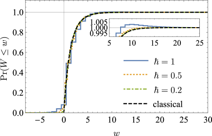
Figure 1: Accumulated distribution of work $\mathrm{Pr}(W\leq w)$. The black dashed curve corresponds to classical work distribution. The discrete distributions with blue solid, orange dotted, and green dot-dashed lines correspond to MH quasiprobability of quantum work with $\hbar=1,0.5,0.2$. The initial squeezed state is prepared with $\gamma_{11}=1$, $\gamma_{22}=1.1$, and $\gamma_{12}=0.9$. The parameters of the harmonic oscillator are chosen as $m=1$, $\omega_{0}=1$ and $\omega_{\tau}=2$, and the operation time is $\tau=1$. The inset shows the negative quasiprobability at relatively large $w$.

In Fig. 1, we show the accumulated distribution of work $\mathrm{Pr}(W\leq w)=\int_{-\infty}^{w}P(w^{\prime})\mathrm{d}w^{\prime}$ with the initial squeezed state in Eq. (25). The parameters are given in the caption of the figure. With the decrease of $\hbar$, the discrete distributions of quantum work (blue solid, orange dotted, and green dot-dashed lines) converge to the classical work distribution (black dashed curve). The convergence shows the quantum-classical correspondence principle of MH quasiprobability of quantum work for initial states with quantum coherence [53].

We remark that a generalized Jarzynski equality has been found for arbitrary initial state [44, 58]. In Refs. [44, 53], the generalized Jarzynski equality is obtained for initial states with quantum coherence as

$$\left\langle\mathrm{e}^{-\beta W}\right\rangle=e^{-\beta\Delta F}\operatorname{Re}\Tr\left[\hat{\rho}\hat{U}^{-1}\hat{\rho}_{\mathrm{eq}}(\tau)U\hat{\rho}_{\mathrm{eq}}(0)^{-1}\right],$$ (39)

where $\hat{\rho}_{\mathrm{eq}}(0)=\mathrm{e}^{-\beta\hat{H}_{S}(0)}/\mathrm{Tr}[\mathrm{e}^{-\beta\hat{H}_{S}(0)}]$ and $\hat{\rho}_{\mathrm{eq}}(\tau)=\mathrm{e}^{-\beta\hat{H}_{S}(\tau)}/\mathrm{Tr}[\mathrm{e}^{-\beta\hat{H}_{S}(\tau)}]$ are equilibrium states with the inverse temperature $\beta$ at the initial and the final time, and $\hat{U}$ is the evolution operator. The conventional Jarzynski equality is recovered for an initial equilibrium state $\hat{\rho}=\hat{\rho}_{\mathrm{eq}}(0)$. With the work distribution obtained in Fig. 1, we can verify the generalized Jarzynski equality (39) by evaluating the two sides separately.

In experiments, the MH quasiprobability can be obtained by the Ramsey scheme [59, 21, 60]. Thus, it is possible to verify the generalized Jarzynski equality for initial states with quantum coherence in future experiments.

VII conclusion and outlook

In this paper, we list several requirements for an appropriate definition of work distribution. Building on the physical implication of the TPM scheme, the support condition is introduced, which reveals that the quantum work corresponds to the transition between the initial and final energy levels, and it plays a crucial role in our proof. Other requirements include the convexity with respect to the initial density operator, the first law of thermodynamics, linear relation on the Hamiltonian, the positivity of second-order moment, and the time-reversal symmetry.

We prove that the MH quasiprobability of quantum work is the only definition that satisfies all the requirements. We also compare some common definitions of quantum work and examine their properties from the perspective of requirements. The FC quasiprobability as well as the $q$-class quasiprobability fails to fulfill the time-reversal symmetry and the support condition due to the asymmetry between the initial and the final Hamiltonians. The KD quasiprobability is also an acceptable definition, which satisfies most of the requirements. Nevertheless, the physical meaning of its imaginary part is unexplored, and the appearance of the imaginary part violates the positivity requirement of the second-order moment. Under all the requirements in this paper, MH quasiprobability of quantum work shows its advantages over other definitions of quantum work.

We explicitly evaluate the MH quasiprobability of quantum work distribution in the example of a breathing harmonic oscillator. The distribution exhibits slightly negative values at the tail. The Jarzynski equality for initial states with quantum coherence [44, 53] is verified in this example.

In addition to the quantum work, other thermodynamic quantities, such as heat and particle number exchange, can also be characterized by quasiprobability if the corresponding operators and the initial density operator do not commute with each other [61, 62, 63]. The requirements in this paper can also help us justify the validity of the MH quasiprobability in such cases. In the study of quantum thermodynamics, one often restricts to the process without initial coherence, in contrast to classical stochastic thermodynamics, where no restriction is put on the process. With the help of the MH quasiprobability, it is promising to handle processes with initial quantum coherence. We will be able to calculate the full counting statistics and characterize the fluctuation for thermodynamic quantities through a standard way in a generic quantum nonequilibrium process. This will provide a solid foundation for related issues such as quantum heat engines and work extractions. In future studies, we hope that the quasiprobability approach can broaden the scope of quantum stochastic thermodynamics.

Appendix A CONVEXITY ON INITIAL STATE AND ITS COROLLARY

In this appendix, we are going to prove that the convexity property (W1) of distribution implies the distribution function $P(w)$ can be expressed as

$$P(w;\rho)=\Tr\left[M(w)\rho\right],$$ (40)

where $M(w)$ is a bounded operator irrelevant to $\rho$.

Before proceeding, we remark that although in the case with $P\geq 0$, this result has been proved [33], there is no strict proof if $P$ is a quasiprobability distribution with real or complex value. Here, we give proof that applies to Hilbert space of any (maybe infinite) dimension.

We now briefly illustrate the outline of the proof. For a specific distribution, we do a linear expansion of $P(w;\rho)$ to $\tilde{P}(w;\tilde{\rho})$, allowing $\tilde{\rho}$ to be any operator that has a definite trace, called trace-class operator. In the trace class, operators are no longer Hermitian or positive. The expanded distribution $\tilde{P}$ becomes a linear function in the trace-class space. Discussions about trace-class space can be found in textbook [64]. The general form of a linear function of the trace-class operator $\tilde{\rho}$ is given by $\Tr[M\tilde{\rho}]$ with $M$ a bounded operator. Therefore, $\tilde{P}$ is represented in this general form, and so is $P$ when restricting to the density operators. In the following, we elaborate on how it works, and the feasibility of the linear expansion will be justified.

We start with a lemma. This lemma is used in the later construction of the linear expansion.
Lemma 1: If a linear combination of several density operators $\rho_{i}$ with real coefficients $\lambda_{i}\in\mathbb{R}$ is zero, that is,

$$\lambda_{1}\rho_{1}+\cdots+\lambda_{N}\rho_{N}=0,$$

then $\lambda_{1}P(w;\rho_{1})+\cdots+\lambda_{N}P(w;\rho_{N})=0$.
Proof: $\rho_{i}$ are all density operators with trace 1, so $0=\lambda_{1}+\cdots+\lambda_{N}$. The case that all the $\lambda_{i}$ equal $0$ is trivial, so we suppose at least one element in $\{\lambda_{i}\}$ is greater than zero. We mark the non-negative terms as $\lambda_{i_{k}},1\leq k\leq M$ and the negative terms as $\lambda_{j_{k}},1\leq k\leq N-M$. We move the term with negative $\lambda_{j_{k}}$ to the right-hand side and rescaling the equation,

$$\frac{1}{\Lambda}\left(\absolutevalue{\lambda_{i_{1}}}\rho_{i_{1}}+\cdots+\absolutevalue{\lambda_{i_{M}}}\rho_{i_{M}}\right)=\frac{1}{\Lambda}\left(\absolutevalue{\lambda_{j_{1}}}\rho_{j_{1}}+\cdots+\absolutevalue{\lambda_{j_{N-M}}}\rho_{j_{N-M}}\right),$$ (41)

where $\Lambda=\absolutevalue{\lambda_{j_{1}}}+\cdots+\absolutevalue{\lambda_{j_{N-M}}}=\absolutevalue{\lambda_{i_{1}}}+\cdots+\absolutevalue{\lambda_{i_{1}}}$. The expression in the above equation is a density operator, which we will denote as $\rho^{\prime}$. Then we split the first term on the left-hand side from the other terms and write it as

$$\rho^{\prime}=\frac{\absolutevalue{\lambda_{i_{1}}}}{\Lambda}\rho_{i_{1}}+\frac{\Lambda-\absolutevalue{\lambda_{i_{1}}}}{\Lambda}\times\frac{1}{\Lambda-\absolutevalue{\lambda_{i_{1}}}}\left(\absolutevalue{\lambda_{i_{2}}}\rho_{i_{2}}+\cdots+\absolutevalue{\lambda_{i_{M}}}\rho_{i_{M}}\right),$$

where $\rho_{i_{1}}$ and $\frac{1}{\Lambda-\absolutevalue{\lambda_{i_{1}}}}\left(\absolutevalue{\lambda_{i_{2}}}\rho_{i_{2}}+\cdots+\absolutevalue{\lambda_{i_{M}}}\rho_{i_{M}}\right)$ are both density operators. From the convexity relation, we get

$$P(w;\rho^{\prime})=\frac{\absolutevalue{\lambda_{i_{1}}}}{\Lambda}P(w;\rho_{i_{1}})+\frac{\Lambda-\absolutevalue{\lambda_{i_{1}}}}{\Lambda}P(w;\frac{\absolutevalue{\lambda_{i_{2}}}\rho_{i_{2}}+\cdots+\absolutevalue{\lambda_{i_{M}}}\rho_{i_{M}}}{\Lambda-\absolutevalue{\lambda_{i_{1}}}}).$$

Next, for density operator $\frac{\absolutevalue{\lambda_{i_{2}}}\rho_{i_{2}}+\cdots+\absolutevalue{\lambda_{i_{M}}}\rho_{i_{M}}}{\Lambda-\absolutevalue{\lambda_{i_{1}}}}$, we continue to split out the first term. After a similar rescaling and applying the convexity relation, we have

$$P(w;\frac{\absolutevalue{\lambda_{i_{2}}}\rho_{i_{2}}+\cdots+\absolutevalue{\lambda_{i_{M}}}\rho_{i_{M}}}{\Lambda-\absolutevalue{\lambda_{i_{1}}}})$$

$$=\frac{\absolutevalue{\lambda_{i_{2}}}}{\Lambda-\absolutevalue{\lambda_{i_{1}}}}P(w;\rho_{i_{2}})+\frac{\Lambda-\absolutevalue{\lambda_{i_{1}}}-\absolutevalue{\lambda_{i_{2}}}}{\Lambda-\absolutevalue{\lambda_{i_{1}}}}P(w;\frac{\absolutevalue{\lambda_{i_{3}}}\rho_{i_{3}}+\cdots+\absolutevalue{\lambda_{i_{M}}}\rho_{i_{M}}}{\Lambda-\absolutevalue{\lambda_{i_{1}}}-\absolutevalue{\lambda_{i_{2}}}}).$$

Repeating the steps to the remaining part, we finally split all the terms apart. The final result is simply

$$\Lambda P(w;\rho^{\prime})=\absolutevalue{\lambda_{i_{1}}}P(w;\rho_{i_{1}})+\cdots+\absolutevalue{\lambda_{i_{M}}}P(w;\rho_{i_{M}}).$$

Similar procedure applies to the right-hand side of Eq. (41),

$$\Lambda P(w;\rho^{\prime})=\absolutevalue{\lambda_{j_{1}}}P(w;\rho_{j_{1}})+\cdots+\absolutevalue{\lambda_{j_{N-M}}}P(w;\lambda_{j_{N-M}}).$$

Combining the two sides and moving the right-hand side back to the left, we complete the proof of the lemma. $\square$

Next, we are going to see that the density operators span the trace class [64], a subspace of the bounded operator space. The trace class is defined by: An operator $A$ belongs to the trace class if and only if $\Tr\absolutevalue{A}<\infty$, where $\absolutevalue{A}=(A^{\dagger}A)^{\frac{1}{2}}$. If $A$ belongs to the trace class, $A$ is called a trace-class operator, which has definite trace $\Tr A$. Obviously, any linear combination of finite number of density operators is a trace-class operator.

On the other hand, let us assume $A$ is a trace-class operator. Every bounded operator can be decomposed into a Hermitian operator plus an anti-Hermitian operator, so we have

$$A=B+\mathrm{i}C,$$

where $B=\frac{1}{2}(A+A^{\dagger}),C=\frac{1}{2\mathrm{i}}(A-A^{\dagger})$ are Hermitian operators. Likewise, both $B$ and $C$ are trace-class operators. Furthermore, bounded Hermitian operators can be decomposed into a subtraction of two positive operators [65]. This applies to $B$ and $C$:

$$B=B_{1}-B_{2},C=C_{1}-C_{2}.$$

By the way, if $B_{1}B_{2}=B_{2}B_{1}=0$ (or $C_{1}C_{2}=C_{2}C_{1}=0$), the decomposition is unique. Meanwhile, positive operators $B_{1},B_{2},C_{1},C_{2}$ are all trace-class operators with finite trace. After a rescaling, operator $A$ is expressed as a linear combination of four density operators.

$$A=\lambda_{1}\rho_{1}-\lambda_{2}\rho_{2}+\mathrm{i}\lambda_{3}\rho_{3}-\mathrm{i}\lambda_{4}\rho_{4},$$ (42)

where $\rho_{1}=B_{1}/\Tr B_{1},\rho_{2}=B_{2}/\Tr B_{2},\rho_{3}=C_{1}/\Tr C_{1},\rho_{4}=C_{2}/\Tr C_{2}$, and all the $\lambda_{i}$ are non-negative number. Therefore, any trace-class operator can be decomposed as the linear combination of 4 density operators (this decomposition is not unique generally), and all the density operators span the trace class.

For a specific distribution function $P(w;\rho)$, we define an expanded distribution $\tilde{P}$ with respect to any trace-class operator $A$ in the following way:

$$\tilde{P}(w;A)=\lambda_{1}P(w;\rho_{1})-\lambda_{2}P(w;\rho_{2})+\mathrm{i}\lambda_{3}P(w;\rho_{3})-\mathrm{i}\lambda_{4}P(w;\rho_{4}),$$ (43)

provided the decomposition in Eq. (42). To serve as a good definition, it should be independent of the choice of decomposition. If there is another different decomposition $A=\lambda_{1}^{\prime}\rho_{1}^{\prime}-\lambda_{2}^{\prime}\rho_{2}^{\prime}+\mathrm{i}\lambda_{3}\rho^{\prime}_{3}-\mathrm{i}\lambda_{4}^{\prime}\rho_{4}^{\prime}$, the expanded distribution under this decomposition is

$$\tilde{P}^{\prime}(w;A)=\lambda_{1}^{\prime}P(w;\rho_{1}^{\prime})-\lambda_{2}^{\prime}P(w;\rho_{2}^{\prime})+\mathrm{i}\lambda_{3}^{\prime}P(w;\rho_{3}^{\prime})-\mathrm{i}\lambda_{4}^{\prime}P(w;\rho_{4}^{\prime}).$$ (44)

In the two different decompositions, the Hermitian part and anti-Hermitian part equal each other respectively, that is, $\lambda_{1}\rho_{1}-\lambda_{2}\rho_{2}=\lambda_{1}^{\prime}\rho_{1}^{\prime}-\lambda_{2}^{\prime}\rho_{2}^{\prime}$ and $\lambda_{3}\rho_{3}-\lambda_{4}\rho_{4}=\lambda_{3}^{\prime}\rho_{3}^{\prime}-\lambda_{4}^{\prime}\rho_{4}^{\prime}$. According to lemma 1, $\lambda_{1}P(\rho_{1})-\lambda_{2}P(\rho_{2})=\lambda_{1}^{\prime}P(\rho_{1}^{\prime})-\lambda_{2}^{\prime}P(\rho_{2}^{\prime})$, $\lambda_{3}P(\rho_{3})-\lambda_{4}P(\rho_{4})=\lambda_{3}^{\prime}P(\rho_{3}^{\prime})-\lambda_{4}^{\prime}P(\rho_{4}^{\prime})$, so the above $P^{\prime}$ coincides with $P$ in Eq. (43). This manifests that the linear expansion is independent of the decomposition. Besides, it is straightforward to verify that the expanded distribution exhibits the standard linear relation that for any complex number $\mu_{1},\mu_{2}$ and trace-class operator $A_{1},A_{2}$,

$$\tilde{P}(w;\mu_{1}A_{1}+\mu_{2}A_{2})=\mu_{1}\tilde{P}(w;A_{1})+\mu_{2}\tilde{P}(w;A_{2}).$$ (45)

Therefore, $\tilde{P}$ is a linear function on the trace class, and we have finished our treatment for the linear expansion.

The dual space (the space of bounded linear function) of the trace class is isomorphic to the bounded operator space [64]. As a linear function of $A$, the expanded distribution $\tilde{P}$ is represented as

$$\tilde{P}(w;A)=\Tr\left[M(w)A\right].$$ (46)

Here $M(w)$ is a bounded operator, which has a one-on-one correspondence with the distribution $\tilde{P}(w)$. If we restrict $A$ to the density matrix $\rho$, $\tilde{P}$ reduces to the work distribution $P$. In this case, we get the final result,

$$P(w;\rho)=\Tr\left[M(w)\rho\right].$$ (47)

Appendix B THE FIRST LAW DETERMINES THE EXPANSION COEFFICIENTS

We are going to specify how to determine the expansion coefficients in Eq. (12) under the condition of the first law of thermodynamics so that the form of $N_{ji}(\Pi_{j}^{1},\Pi_{i}^{0})$ is fixed to Eq. (15). In addition, we will verify the time-reversal symmetry for the $N_{ji}$ in Eq. (15).

We have obtained the condition for $N_{ij}$ from the first law in Eq. (14), which is also listed below:

$$\sum_{ij}(\epsilon_{j}^{1}-\epsilon_{i}^{0})N_{ji}=H_{1}-H_{0}=\sum_{j}\epsilon_{j}^{1}\Pi_{j}^{1}-\sum_{i}\epsilon_{i}^{0}\Pi_{i}^{0}.$$ (48)

Since the first law is valid in arbitrary protocols, we have the liberty to assign the values of $\epsilon_{j}^{1},\Pi_{j}^{1},\epsilon_{i}^{0},\Pi_{i}^{0}$. Due to the arbitrariness of $\epsilon_{j}^{1},\epsilon_{i}^{0}$, the above equation is equivalent to

$$\sum_{i}N_{ji}=\Pi_{j}^{1},\;\sum_{j}N_{ji}=\Pi_{i}^{0}.$$

Noticing in the MH work quasiprobability, $N_{ij}^{\textit{MH}}=\frac{1}{2}(\Pi_{j}^{1}\Pi_{i}^{0}+\Pi_{i}^{0}\Pi_{j}^{1})$ obviously satisfies the above equation, we adopt a trick here. We consider $\tilde{N}_{ij}=N_{ij}-N_{ij}^{\textit{MH}}$ instead, and a tilde is used for $\tilde{N}_{ij}$ in the same expansion as Eq. (12). That is,

$$\tilde{N}_{ji}(\Pi_{j}^{1},\Pi_{i}^{0})=\tilde{e}_{0}I+\sum_{n=1}^{\infty}[\tilde{a}_{n}(\Pi_{j}^{1}\Pi_{i}^{0})^{n}+\tilde{b}_{n}(\Pi_{i}^{0}\Pi_{j}^{1})^{n}]+\sum_{n=0}^{\infty}[\tilde{c}_{n}\Pi_{i}^{0}(\Pi_{j}^{1}\Pi_{i}^{0})^{n}+\tilde{d}_{n}(\Pi_{j}^{1}\Pi_{i}^{0})^{n}\Pi_{j}^{1}].$$ (49)

The condition for $\tilde{N}_{ij}$ now changes to

$$\sum_{i}\tilde{N}_{ji}=0,\sum_{j}\tilde{N}_{ji}=0.$$ (50)

It is enough to find a specific set of $\Pi_{j}^{1},\Pi_{i}^{0}$, under which all the $\tilde{a}_{n},\tilde{c}_{n}$ are fixed to be our desired values. We will show how this works in the separable Hilbert space with dimension $2<d\leq\infty$.

For the sake of clarity, in this section, we denote the initial eigenstates as $\ket{\psi_{m}},1\leq m\leq d$, and the final eigenstates as $\ket{\phi_{m}}$, instead of $\ket{\psi^{0}_{m}},\ket{\psi^{1}_{m}}$. The projective operators corresponding to these eigenstates are

$$\Pi_{i}^{0}=\outerproduct{\psi_{i}}{\psi_{i}},\Pi_{j}^{1}=\outerproduct{\phi_{j}}{\phi_{j}}.$$

Direct calculation of each term in the expansion yields

$$(\Pi^{1}_{j}\Pi^{0}_{i})^{n}=\innerproduct{\phi_{j}}{\psi_{i}}^{n}\innerproduct{\psi_{i}}{\phi_{j}}^{n-1}\outerproduct{\phi_{j}}{\psi_{i}},$$

$$(\Pi^{0}_{i}\Pi^{1}_{j})^{n}=\innerproduct{\phi_{j}}{\psi_{i}}^{n-1}\innerproduct{\psi_{i}}{\phi_{j}}^{n}\outerproduct{\psi_{i}}{\phi_{j}},$$

$$\Pi^{0}_{i}(\Pi^{1}_{j}\Pi^{0}_{i})^{n}=\innerproduct{\phi_{j}}{\psi_{i}}^{n}\innerproduct{\psi_{i}}{\phi_{j}}^{n}\outerproduct{\psi_{i}}{\psi_{i}},$$

$$(\Pi^{1}_{j}\Pi^{0}_{i})^{n}\Pi^{1}_{j}=\innerproduct{\phi_{j}}{\psi_{i}}^{n}\innerproduct{\psi_{i}}{\phi_{j}}^{n}\outerproduct{\phi_{j}}{\phi_{j}}.$$

For $2<d\leq\infty$, our specific set of eigenstates are chosen as follows. The initial energy eigenstates are selected to be the standard basis, that is, only the $m$-th component is nonzero,

$$\ket{\psi_{m}}=(0,\dots,0,\overset{m}{1},0,\dots).$$ (51)

As for final energy eigenstates, the first three states are some real vectors:

$$\ket{\phi_{1}}=( \sin\theta\cos\phi, \sin\theta\sin\phi, \cos\theta, 0,\dots ),$$ (52)

$$\ket{\phi_{2}}=( \cos\theta\cos\phi, \cos\theta\sin\phi, -\sin\theta, 0,\dots ),$$

$$\ket{\phi_{3}}=( -\sin\phi, \cos\phi, 0, 0,\dots ).$$

Other final energy eigenstates are the same as the initial ones,

$$\ket{\phi_{m}}=\ket{\psi_{m}},\quad\text{for }m>3.$$ (53)

Also, the whole final energy eigenstates form a set of orthogonal basis in the Hilbert space.

Let us consider the following matrix element of the Eq. (50),

$$\sum_{j=1}^{d}\expectationvalue{\tilde{N}_{j1}}{\psi_{2}}=0.$$ (54)

Substituting Eqs. (49), (52) in the above equation, we find only one kind of terms in the expansion survives besides the identity, and the explicit expression reads

$$d\tilde{e}_{0}+\sum_{n=0}^{\infty}\tilde{d}_{n}[(\sin\theta\cos\phi)^{2n}(\sin\theta\sin\phi)^{2}+(\cos\theta\cos\phi)^{2n}(\cos\theta\sin\phi)^{2}+(-\sin\phi)^{2n}(\cos\phi)^{2}]=0.$$ (55)

To make it clear, we introduce $x=\cos^{2}\theta$, $1-x=\sin^{2}\theta$, $y=\cos^{2}\phi$, $1-y=\sin^{2}\phi$ and obtain

$$d\tilde{e}_{0}+\sum_{n=0}^{\infty}\tilde{d}_{n}F_{n}(x,y)=0,$$ (56)

where $F_{n}(x,y)=[(1-x)^{n+1}y^{n}(1-y)+x^{n+1}y^{n}(1-y)+y(1-y)^{n}]$, and the above equation holds for any $0<x,y<1$. For a specific value $x=\frac{1}{2}$, we have

$$F_{n}(\frac{1}{2},y)=\frac{1}{2^{n}}y^{n}(1-y)+y(1-y)^{n}.$$ (57)

For $n>0$, $F_{n}(1/2,y)$ is a polynomial of $y$ with degree $n+1$, while for $n=0$, $F_{0}=1$. Therefore, $F_{n}$ with different $n$ are linearly independent. According to Eq. (56), we find $\tilde{d}_{n}=0$ for $n>0$, and $\tilde{d}_{0}=-d\tilde{e}_{0}$. Here, $d$ is the dimension of the Hilbert space. If considering $\sum_{j=1}^{d}\expectationvalue{\tilde{N}_{1j}}{\phi_{2}}=0$, the similar derivation leads to $\tilde{c}_{n}=0,n>0$ and $\tilde{c}_{0}=-d\tilde{e}_{0}$.

Next, we investigate the following matrix element to find the relation of $\tilde{a}_{n}$,

$$\sum_{j=1}^{d}\matrixelement{\psi_{2}}{\tilde{N}_{j1}}{\psi_{1}}=0.$$ (58)

In explicit form, we have

$$\sum_{n=1}^{\infty}\tilde{a}_{n}[(\sin\theta\cos\phi)^{2n-1}\sin\theta\sin\phi+(\cos\theta\cos\phi)^{2n-1}\cos\theta\sin\phi+(-\sin\phi)^{2n-1}\cos\phi]=0.$$ (59)

As long as $0<\phi<\pi/2$, we can eliminate the common factor $\sin\phi\cos\phi$ in the above equation and obtain

$$\sum_{n=1}^{\infty}\tilde{a}_{n}G_{n}(x,y)=0,$$ (60)

where $G_{n}(x,y)=[x^{n}y^{n-1}+(1-x)^{n}y^{n-1}-(1-y)^{n-1}]$, and $x=\cos^{2}\theta,y=\cos^{2}\phi$ again. The above equation is valid for any $0<x,y<1$. We find that $G_{1}=0$ for any value of $x,y$. Assigning a specific value $x=\frac{1}{2}$, $G_{n}$ reduces to

$$G_{n}(\frac{1}{2},y)=\frac{1}{2^{n-1}}y^{n-1}-(1-y)^{n-1}.$$ (61)

For $n>1$, $G_{n}(1/2,y)$ is a polynomial of $y$ with degree $n-1$. $\{G_{n}\},(n>1)$ are linearly independent, so $\tilde{a}_{n}=0$ for $n>1$ according to Eq. (60). Since $G_{1}=0$, this equation puts no constraint on $\tilde{a}_{1}$. Likewise, if we consider $\sum_{j=1}^{d}\matrixelement{\psi_{1}}{\tilde{N}_{j1}}{\psi_{2}}=0$ instead, we can deduce that $\tilde{b}_{n}=0$ for $n>1$ while $\tilde{b}_{1}$ is free.

The remaining unknown coefficients are $\tilde{a}_{1},\tilde{b}_{1}$. Let us consider

$$\sum_{j=1}^{d}\expectationvalue{\tilde{N}_{j1}}{\psi_{1}}=0.$$ (62)

After some simple calculations, we find the relation between $\tilde{a}_{1},\tilde{b}_{1}$:

$$\tilde{a}_{1}+\tilde{b}_{1}=d^{2}\tilde{e}_{0}.$$ (63)

Up to now, the expansion for $\tilde{N}_{ji}$ is fixed to

$$\tilde{N}_{ji}(\Pi^{1}_{j},\Pi^{0}_{i})=\tilde{e}_{0}I-d\tilde{e}_{0}[\Pi^{0}_{i}+\Pi^{1}_{j}]+\tilde{a}_{1}\Pi^{1}_{j}\Pi^{0}_{i}+(-\tilde{a}_{1}+d^{2}\tilde{e}_{0})\Pi^{0}_{i}\Pi^{1}_{j},$$ (64)

with free coefficients $\tilde{e}_{0},\tilde{a}_{1}$. On the other hand, it can be checked that the above expression satisfies the condition for $\tilde{N}_{ji}$ in Eq. (50), so it may be regarded as the general form of $\tilde{N}_{ji}$. However, we hope the definition of work is universal and irrespective of the dimension of Hilbert space $d$. Especially, the above expression should work well in infinite-dimensional space. Therefore, we are forced to choose $\tilde{e}_{0}=0$. By the way, we find that 2-dimensional Hilbert space is an exception because we have less freedom to choose the projective operators. Nevertheless, since the definition should be universal irrespective of the dimension, this exception in 2d space does not matter.

In conclusion, under the condition from the first law, the general form for $N_{ji}$ is simply

$$N_{ji}(\Pi^{1}_{j},\Pi^{0}_{i})=\frac{1+\eta}{2}\Pi^{1}_{j}\Pi^{0}_{i}+\frac{1-\eta}{2}\Pi^{0}_{i}\Pi^{1}_{j},$$ (65)

where $\eta=2\tilde{a}_{1}$ can be arbitrary complex number. The corresponding distribution function reads

$$P(w)=\sum_{ji}\delta(w-(\epsilon^{1}_{j}-\epsilon^{0}_{i}))\Tr\left[\left(\frac{1+\eta}{2}\Pi^{1}_{j}\Pi^{0}_{i}+\frac{1-\eta}{2}\Pi^{0}_{i}\Pi^{1}_{j}\right)\rho\right].$$ (66)

This form contains the MH quasiprobability for work ($\eta=0$) and the KD quasiprobability for work ($\eta=1$).

At the end of this appendix, we will show that the above distribution satisfies time-reversal symmetry (E2). In the time-reversed process described in requirement (E2), we have the following relations in the Heisenberg picture: $\bar{H}_{1}=\Theta UH_{0}U^{-1}\Theta^{-1},\bar{H}_{0}=\Theta UH_{1}U^{-1}\Theta^{-1}$, $\bar{\rho}=\Theta U\rho U^{-1}\Theta^{-1}$. The eigenvalues and corresponding projective operators are: $\bar{\epsilon}^{0}_{i}=\epsilon^{1}_{i},\bar{\epsilon}^{1}_{j}=\epsilon^{0}_{j}$, $\bar{\Pi}^{0}_{i}=\Theta U\Pi^{1}_{i}U^{-1}\Theta^{-1},\bar{\Pi}^{1}_{j}=\Theta U\Pi^{0}_{j}U^{-1}\Theta^{-1}$. Operator $N_{ji}$ now changes to

$$N_{ji}(\bar{\Pi}^{1}_{j},\bar{\Pi}^{0}_{i})=\Theta UN_{ji}^{*}(\Pi^{0}_{j},\Pi^{1}_{i})U^{-1}\Theta^{-1},$$

where superscript $*$ on $N_{ji}$ denotes the complex conjugate over all the coefficients in the expansion of $N_{ji}$. After some derivation, we get the distribution function in the time-reversed process:

$$\bar{P}(w) =\sum_{ji}\delta(w-(\bar{\epsilon}^{1}_{j}-\bar{\epsilon}^{0}_{i}))\Tr[N_{ji}(\bar{\Pi}^{1}_{j},\bar{\Pi}^{0}_{i})\bar{\rho}]$$ (67)

$$=\sum_{ji}\delta(w-(\epsilon^{0}_{j}-\epsilon^{1}_{i}))\Tr[N_{ji}^{*}(\Pi^{0}_{j},\Pi^{1}_{i})\rho]^{*}$$

$$=\sum_{ji}\delta(w+(\epsilon^{1}_{j}-\epsilon^{0}_{i}))\Tr[N_{ij}^{*\dagger}(\Pi^{0}_{i},\Pi^{1}_{j})\rho].$$

In the second equality, please notice that when canceling the anti-unitary operator $\Theta$ in the trace, there will be an extra complex conjugate. In the third equality, we exchange the summation index $i,j$. Imposing $\bar{P}(w)=P(-w)$, we find that the time-reversal condition on $N_{ji}$ is

$$N_{ij}^{*\dagger}(\Pi^{0}_{i},\Pi^{1}_{j})=N_{ji}(\Pi^{1}_{j},\Pi^{0}_{i}).$$ (68)

In terms of expansion coefficients in Eq. (12), we find that $c_{n}=d_{n}$ while there are no constraints on $a_{n},b_{n}$. $N_{ji}$ in Eq. (66) satisfies this condition. Particularly, both the MH quasiprobability of work and the KD quasiprobability of work encode the time-reversal symmetry. Thus, the time-reversal symmetry property (E2) can be regarded as a consequence of other requirements.

References

- Seifert [2012] U. Seifert, Stochastic thermodynamics, fluctuation theorems and molecular machines, Rep. Prog. Phys. 75, 126001 (2012).
- Peliti and Pigolotti [2021] L. Peliti and S. Pigolotti, Stochastic Thermodynamics: An Introduction (Princeton University Press, 2021).
- Sekimoto [2010] K. Sekimoto, Stochastic energetics, Vol. 799 (Springer, 2010).
- Jarzynski [2011] C. Jarzynski, Equalities and inequalities: Irreversibility and the second law of thermodynamics at the nanoscale, Annu. Rev. Conden. Matt. Phys. 2, 329 (2011).
- Vinjanampathy and Anders [2016] S. Vinjanampathy and J. Anders, Quantum thermodynamics, Contemp. Phys. 57, 545 (2016), https://doi.org/10.1080/00107514.2016.1201896 .
- Pekola [2015] J. P. Pekola, Towards quantum thermodynamics in electronic circuits, Nat. Phys. 11, 118 (2015).
- Strasberg [2022] P. Strasberg, Quantum Stochastic Thermodynamics: Foundations and Selected Applications (Oxford University Press, 2022) https://academic.oup.com/book/43799/book-pdf/50145705/9780192648143_web.pdf .
- Goold et al. [2016] J. Goold, M. Huber, A. Riera, L. del Rio, and P. Skrzypczyk, The role of quantum information in thermodynamics—a topical review, J. Phys. A: Math. Theor. 49, 143001 (2016).
- Åberg [2018] J. Åberg, Fully quantum fluctuation theorems, Phys. Rev. X 8, 011019 (2018).
- Campisi et al. [2015] M. Campisi, J. Pekola, and R. Fazio, Nonequilibrium fluctuations in quantum heat engines: theory, example, and possible solid state experiments, New J. Phys. 17, 035012 (2015).
- Millen and Xuereb [2016] J. Millen and A. Xuereb, Perspective on quantum thermodynamics, New J. Phys. 18, 011002 (2016).
- Manzano et al. [2018] G. Manzano, J. M. Horowitz, and J. M. R. Parrondo, Quantum fluctuation theorems for arbitrary environments: Adiabatic and nonadiabatic entropy production, Phys. Rev. X 8, 031037 (2018).
- Talkner and Hänggi [2016] P. Talkner and P. Hänggi, Aspects of quantum work, Phys. Rev. E 93, 022131 (2016).
- Bochkov and Kuzovlev [1977] G. Bochkov and Y. Kuzovlev, General theory of thermal fluctuations in nonlinear systems, Zh. Eksp. Teor. Fiz 72, 238 (1977).
- Allahverdyan and Nieuwenhuizen [2005] A. E. Allahverdyan and T. M. Nieuwenhuizen, Fluctuations of work from quantum subensembles: The case against quantum work-fluctuation theorems, Phys. Rev. E 71, 066102 (2005).
- Kurchan [2001] J. Kurchan, A quantum fluctuation theorem (2001), arXiv:cond-mat/0007360 [cond-mat.stat-mech] .
- Tasaki [2000] H. Tasaki, Jarzynski relations for quantum systems and some applications (2000), arXiv:cond-mat/0009244 [cond-mat.stat-mech] .
- Talkner et al. [2009] P. Talkner, M. Campisi, and P. Hänggi, Fluctuation theorems in driven open quantum systems, J. Stat. Mech: Theory Exp. 2009, P02025 (2009).
- Esposito et al. [2009] M. Esposito, U. Harbola, and S. Mukamel, Nonequilibrium fluctuations, fluctuation theorems, and counting statistics in quantum systems, Rev. Mod. Phys. 81, 1665 (2009).
- Campisi et al. [2011] M. Campisi, P. Hänggi, and P. Talkner, Colloquium: Quantum fluctuation relations: Foundations and applications, Rev. Mod. Phys. 83, 771 (2011).
- Batalhão et al. [2014] T. B. Batalhão, A. M. Souza, L. Mazzola, R. Auccaise, R. S. Sarthour, I. S. Oliveira, J. Goold, G. De Chiara, M. Paternostro, and R. M. Serra, Experimental reconstruction of work distribution and study of fluctuation relations in a closed quantum system, Phys. Rev. Lett. 113, 140601 (2014).
- An et al. [2015] S. An, J.-N. Zhang, M. Um, D. Lv, Y. Lu, J. Zhang, Z.-Q. Yin, H. T. Quan, and K. Kim, Experimental test of the quantum jarzynski equality with a trapped-ion system, Nat. Phys. 11, 193 (2015).
- Roßnagel et al. [2014] J. Roßnagel, O. Abah, F. Schmidt-Kaler, K. Singer, and E. Lutz, Nanoscale heat engine beyond the carnot limit, Phys. Rev. Lett. 112, 030602 (2014).
- Brandner et al. [2017] K. Brandner, M. Bauer, and U. Seifert, Universal coherence-induced power losses of quantum heat engines in linear response, Phys. Rev. Lett. 119, 170602 (2017).
- Klatzow et al. [2019] J. Klatzow, J. N. Becker, P. M. Ledingham, C. Weinzetl, K. T. Kaczmarek, D. J. Saunders, J. Nunn, I. A. Walmsley, R. Uzdin, and E. Poem, Experimental demonstration of quantum effects in the operation of microscopic heat engines, Phys. Rev. Lett. 122, 110601 (2019).
- Uzdin et al. [2015] R. Uzdin, A. Levy, and R. Kosloff, Equivalence of quantum heat machines, and quantum-thermodynamic signatures, Phys. Rev. X 5, 031044 (2015).
- Watanabe et al. [2017] G. Watanabe, B. P. Venkatesh, P. Talkner, and A. del Campo, Quantum performance of thermal machines over many cycles, Phys. Rev. Lett. 118, 050601 (2017).
- Ma et al. [2021] Y.-H. Ma, C. L. Liu, and C. P. Sun, Works with quantum resource of coherence (2021), arXiv:2110.04550 [quant-ph] .
- Chen et al. [2019a] J.-F. Chen, C.-P. Sun, and H. Dong, Boosting the performance of quantum otto heat engines, Phys. Rev. E 100, 032144 (2019a).
- Chen et al. [2019b] J.-F. Chen, C.-P. Sun, and H. Dong, Achieve higher efficiency at maximum power with finite-time quantum otto cycle, Phys. Rev. E 100, 062140 (2019b).
- Perarnau-Llobet et al. [2015] M. Perarnau-Llobet, K. V. Hovhannisyan, M. Huber, P. Skrzypczyk, N. Brunner, and A. Acín, Extractable work from correlations, Phys. Rev. X 5, 041011 (2015).
- Korzekwa et al. [2016] K. Korzekwa, M. Lostaglio, J. Oppenheim, and D. Jennings, The extraction of work from quantum coherence, New J. Phys. 18, 023045 (2016).
- Perarnau-Llobet et al. [2017] M. Perarnau-Llobet, E. Bäumer, K. V. Hovhannisyan, M. Huber, and A. Acin, No-go theorem for the characterization of work fluctuations in coherent quantum systems, Phys. Rev. Lett. 118, 070601 (2017).
- Lostaglio [2018] M. Lostaglio, Quantum fluctuation theorems, contextuality, and work quasiprobabilities, Phys. Rev. Lett. 120, 040602 (2018).
- Wigner [1932] E. Wigner, On the quantum correction for thermodynamic equilibrium, Phys. Rev. 40, 749 (1932).
- Kirkwood [1933] J. G. Kirkwood, Quantum statistics of almost classical assemblies, Phys. Rev. 44, 31 (1933).
- Dirac [1945] P. A. M. Dirac, On the analogy between classical and quantum mechanics, Rev. Mod. Phys. 17, 195 (1945).
- Margenau and Hill [1961] H. Margenau and R. N. Hill, Correlation between measurements in quantum theory, Prog. Theor. Phys. 26, 722 (1961), https://academic.oup.com/ptp/article-pdf/26/5/722/5454875/26-5-722.pdf .
- Francica and Dell’Anna [2023] G. Francica and L. Dell’Anna, Quasiprobability distribution of work in the ising model (2023), arXiv:2302.11255 [quant-ph] .
- Santini et al. [2023] A. Santini, A. Solfanelli, S. Gherardini, and M. Collura, Work statistics, quantum signatures and enhanced work extraction in quadratic fermionic models (2023), arXiv:2302.13759 [quant-ph] .
- Lostaglio et al. [2022] M. Lostaglio, A. Belenchia, A. Levy, S. Hernández-Gómez, N. Fabbri, and S. Gherardini, Kirkwood-dirac quasiprobability approach to quantum fluctuations: Theoretical and experimental perspectives (2022), arXiv:2206.11783 [quant-ph] .
- Ortega et al. [2019] A. Ortega, E. McKay, A. M. Alhambra, and E. Martín-Martínez, Work distributions on quantum fields, Phys. Rev. Lett. 122, 240604 (2019).
- Teixidó-Bonfill et al. [2020] A. Teixidó-Bonfill, A. Ortega, and E. Martín-Martínez, First law of quantum field thermodynamics, Phys. Rev. A 102, 052219 (2020).
- Allahverdyan [2014] A. E. Allahverdyan, Nonequilibrium quantum fluctuations of work, Phys. Rev. E 90, 032137 (2014).
- Solinas and Gasparinetti [2015] P. Solinas and S. Gasparinetti, Full distribution of work done on a quantum system for arbitrary initial states, Phys. Rev. E 92, 042150 (2015).
- Nazarov and Kindermann [2003] Y. V. Nazarov and M. Kindermann, Full counting statistics of a general quantum mechanical variable, The European Physical Journal B - Condensed Matter and Complex Systems 35, 413 (2003).
- Francica [2022a] G. Francica, Class of quasiprobability distributions of work with initial quantum coherence, Phys. Rev. E 105, 014101 (2022a).
- Francica [2022b] G. Francica, Most general class of quasiprobability distributions of work, Phys. Rev. E 106, 054129 (2022b).
- Miller and Anders [2017] H. J. D. Miller and J. Anders, Time-reversal symmetric work distributions for closed quantum dynamics in the histories framework, New J. Phys. 19, 062001 (2017).
- Sampaio et al. [2018] R. Sampaio, S. Suomela, T. Ala-Nissila, J. Anders, and T. G. Philbin, Quantum work in the bohmian framework, Phys. Rev. A 97, 012131 (2018).
- Sagawa [2013] T. Sagawa, Second law-like inequalities with quantum relative entropy: An introduction, in Lectures on quantum computing, thermodynamics and statistical physics (World Scientific, 2013) pp. 125–190.
- Bäumer et al. [2018] E. Bäumer, M. Lostaglio, M. Perarnau-Llobet, and R. Sampaio, Fluctuating work in coherent quantum systems: Proposals and limitations, in Thermodynamics in the Quantum Regime: Fundamental Aspects and New Directions, edited by F. Binder, L. A. Correa, C. Gogolin, J. Anders, and G. Adesso (Springer International Publishing, Cham, 2018) pp. 275–300.
- Pan et al. [2019] R. Pan, Z. Fei, T. Qiu, J.-N. Zhang, and H. T. Quan, Quantum-classical correspondence of work distributions for initial states with quantum coherence (2019), arXiv:1904.05378 [quant-ph] .
- Beau et al. [2016] M. Beau, J. Jaramillo, and A. Del Campo, Scaling-up quantum heat engines efficiently via shortcuts to adiabaticity, Entropy 18, 10.3390/e18050168 (2016).
- Lee et al. [2021] S. Lee, M. Ha, and H. Jeong, Quantumness and thermodynamic uncertainty relation of the finite-time otto cycle, Phys. Rev. E 103, 022136 (2021).
- Fei et al. [2022] Z. Fei, J.-F. Chen, and Y.-H. Ma, Efficiency statistics of a quantum otto cycle, Phys. Rev. A 105, 022609 (2022).
- Fei and Quan [2019] Z. Fei and H. T. Quan, Group-theoretical approach to the calculation of quantum work distribution, Phys. Rev. Res. 1, 033175 (2019).
- Gong and Quan [2015] Z. Gong and H. T. Quan, Jarzynski equality, crooks fluctuation theorem, and the fluctuation theorems of heat for arbitrary initial states, Phys. Rev. E 92, 012131 (2015).
- Dorner et al. [2013] R. Dorner, S. R. Clark, L. Heaney, R. Fazio, J. Goold, and V. Vedral, Extracting quantum work statistics and fluctuation theorems by single-qubit interferometry, Phys. Rev. Lett. 110, 230601 (2013).
- Mazzola et al. [2013] L. Mazzola, G. De Chiara, and M. Paternostro, Measuring the characteristic function of the work distribution, Phys. Rev. Lett. 110, 230602 (2013).
- Manzano et al. [2022] G. Manzano, J. M. Parrondo, and G. T. Landi, Non-abelian quantum transport and thermosqueezing effects, PRX Quantum 3, 010304 (2022).
- Yunger Halpern et al. [2016] N. Yunger Halpern, P. Faist, J. Oppenheim, and A. Winter, Microcanonical and resource-theoretic derivations of the thermal state of a quantum system with noncommuting charges, Nature Communications 7, 12051 (2016).
- Majidy et al. [2023] S. Majidy, W. F. Braasch, A. Lasek, T. Upadhyaya, A. Kalev, and N. Y. Halpern, Noncommuting conserved charges in quantum thermodynamics and beyond (2023), arXiv:2306.00054 [quant-ph] .
- Conway [2007a] J. B. Conway, Normal operators on hilbert space, in A Course in Functional Analysis (Springer New York, New York, NY, 2007) pp. 255–302.
- Conway [2007b] J. B. Conway, Operators on hilbert space, in A Course in Functional Analysis (Springer New York, New York, NY, 2007) pp. 26–62.