Finite-Temperature Screw Dislocation Core Structures and Dynamics in $\alpha$-Titanium

Abstract

A multiscale approach based on molecular dynamics (MD) and kinetic Monte Carlo (kMC) methods is developed to simulate the dynamics of an $\langle\mathbf{a}\rangle$ screw dislocation in $\alpha$-Ti. The free energy barriers for the core dissociation transitions and Peierls barriers for dislocation glide as a function of temperature are extracted from the MD simulations (based on Machine Learning interatomic potentials and optimization); these form the input to kMC simulations. Random walk dislocation trajectories from kMC agree well with those predicted by MD. On some planes, dislocations move via a locking-unlocking mechanism. Surprisingly, some dislocations glide in directions that are not parallel with the core dissociation direction. The MD/kMC multiscale method proposed is applicable to dislocation motion in simple and complex materials (not only screw dislocations in Ti) as a function of temperature and stress state.

I Introduction

The major plastic deformation mechanism in crystalline metals is dislocation glide. The motion of dislocations is (largely) controlled by elastic stresses and intrinsic dislocation properties. While these stresses are easily analyzed in terms of continuum elasticity, dislocation motion often occurs preferentially on planes other than those with the largest resolved shear stress. This is associated with differences in glide resistance/lattice friction between different slip planes. This depends on the relative ease with which the dislocation core moves. The ease of glide, in turn, is sensitive to the dislocation core structure [1, 2, 3, 4, 5, 6]. The dislocation core structure is, in many cases, temperature-dependent. While knowledge of the core structure is essential, a quantitative link between core structure and dislocation dynamics is often elusive. Here, we develop a multiscale approach to predict screw dislocation dynamics in $\alpha$-Ti.

Atomistic simulations are commonly employed to determine dislocation core structure, in part because the direct experimental determination of the structure is demanding [7]. Since the atomic structure of the material is highly distorted with respect to that in a perfect crystal, quantum mechanical accuracy is often required to predict core structures; often achieved using density functional theory (DFT) calculations [8, 9, 10, 11]. Transition state theory-based methods (such as the nudged elastic band NEB method) are often employed to discern the minimum energy path of a dislocation core as it traverses the slip plane [12, 10, 11, 13]. While DFT methods are usually limited to ground-state (0 K) structures, finite-temperature ab initio molecular dynamics are possible but too computationally costly for widespread use. Therefore, most finite-temperature dislocation core structure determination is based upon semi-empirical interatomic potential methods; e.g., Poschmann et al. [14] studied the core structure of an $\langle\mathbf{a}\rangle=a\langle 10\overline{1}0\rangle$ screw dislocation in $\alpha$-Ti at finite temperature using a modified embedded atom method (MEAM) potential [15]. Unfortunately, this MEAM potential fails to accurately reproduce all of the relevant 0 K core structures and energies predicted by DFT [16]. Bond order potentials (BOPs) [17, 18] were proposed to retain the quantum nature of atomic interactions in transition metals in a more cost-effective manner than DFT. However, BOPs are both computationally costly and not easily implemented in molecular dynamics (MD) simulations [19]. The recently developed Deep Potentials (DPs) [20, 21] (a class of neural network potential) yield DFT accuracy with near empirical potential computational efficiency. Here, we employ the DP method to predict the structure of screw dislocation cores at finite-temperature in $\alpha$-Ti.

The link between dislocation core structure and dislocation dynamics is often related to the assumption that the dislocation glide direction is consistent with the dislocation core dissociation direction. While such an assumption may be valid in some simple cases, its validity is far from assured in the case of more complex (non-cubic) materials, such as hexagonal close packed (HCP) metals. Several models have been proposed to simulate dislocation dynamics at the mesoscale, such as discrete dislocation dynamics (DDD) [22, 23, 24] and kinetic Monte Carlo (kMC) [25, 26, 27, 28, 23] methods. Extant mesoscale models do not explicitly incorporate the effects associated with the dislocation core structure. Here, we develop a mesoscale dislocation dynamics model that incorporates an explicit description of the atomic-scale character of dislocation core structure.

While recent simulations (e.g., see [14]) focus on long dislocation lines, here we focus on the intrinsic dislocation properties associated with the dislocation core structure. The admittedly important roles played by dislocation kinks in the motion of long dislocations are omitted here in order to provide a thorough examination of core effects without the complicated features of kink dynamics (which vary dramatically with, e.g., local dislocation curvature, junctions and interactions with other dislocations). The effects of core structure of short $\langle\mathbf{a}\rangle$ screw dislocation segments in $\alpha$-Ti based on the DP for Ti as a function of temperature are investigated. Experimental observations [29] show that the edge dislocations are highly mobile and the yield strength of HCP Ti is governed by screw dislocation lattice friction. We report the results of MD simulations (based on machine learning potentials of quantum mechanical accuracy) of screw dislocation core structures, transitions between different core structures, statistical analysis of dislocation motion, and the determination of the kinetic parameters (i.e., free energy barriers associated with migration, core structure transitions, …) describing screw dislocation motion. We then perform kinetic Monte Carlo simulations of screw dislocation motion in Ti incorporating these quantum mechanically accurate MD simulation parameters. We examine the effect of both temperature and loading direction on dislocation core transitions and dislocation mobility. The results provide the basis for understanding non-Arrhenius screw dislocation mobility in metals with complex crystal structures.

II Atomistic dislocation structure and dynamics

II.1 Dislocation Core Structure

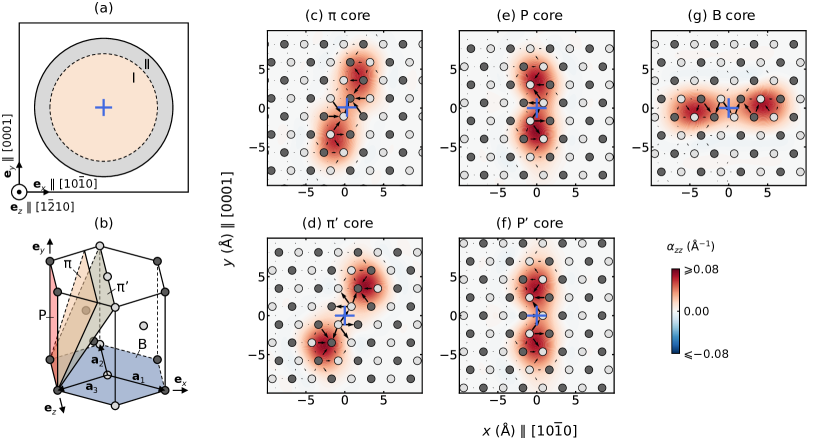
Figure 1: MD simulations of the $\langle\mathbf{a}\rangle$ dislocation core structure in $\alpha$-Ti. (a) The cylindrical model and Cartesian coordinate system employed in the MD simulations. The blue “$+$” symbol indicates where the screw dislocation was introduced. The atomic interaction in Region I and Region II are all modeled using DP, while atoms in Region II are treated via an Einstein model. (b) An HCP unit cell, where the P,   1 0 -.25 1$\pi$, $\mbox{\hskip 5.70027pt{1 0 -.25 1}\hbox to0.0pt{\hss\leavevmode\hbox{\set@color$\pi$}}}^{\prime}$ and B planes are identified. (c)-(g) The dislocation cores observed in the MD simulations (following 10-20 energy minimization steps – for improved visualization, see Method and Ref. [23]). The dark and light gray circles denote atoms on successive $(1\bar{2}10)$ planes (perpendicular to the $\mathbf{e}_{z}$-axis) in the perfect crystal. The arrows represent the differential displacement map while the color heat map shows the $\alpha_{zz}$ distribution. Blue “$+$” symbols indicate the core positions determined by the first moment of $\alpha_{zz}$.

We performed MD simulations to determine $\langle\mathbf{a}\rangle$ screw dislocation core structure in $\alpha$-Ti; the simulation geometry is shown in Fig. 1a (see Methods). By examining all the MD configurations from 300-900 K, we identified five distinct core structures for the $\langle\mathbf{a}\rangle$ screw dislocation in HCP Ti. Figure. 1c-g show these five core structures with a differential displacement map [30] (the black arrows) and the Nye tensor component $\alpha_{zz}$ [31, 32] (the contour). The $\alpha_{zz}$ map describes the screw component of the Burgers vector density. We find that the distribution of $\alpha_{zz}$ is highly delocalized in the form of a dipole, indicating that the core structure dissociates on a plane that includes $[1\bar{2}10]$. For convenience, we denote the pyramidal plane by “  1 0 -.25 1$\pi$”, the prismatic plane by “P” and the basal plane by “B”. We find that two of the dislocation cores dissociate along the   1 0 -.25 1$\pi$ plane; i.e., the “  1 0 -.25 1$\pi$ core” (Fig. 1c) and “$\mbox{\hskip 5.70027pt{1 0 -.25 1}\hbox to0.0pt{\hss\leavevmode\hbox{\set@color$\pi$}}}^{\prime}$ core” (Fig. 1d). The dissociation plane of   1 0 -.25 1$\pi$ core is close to $(\bar{3}031)$ while that of $\mbox{\hskip 5.70027pt{1 0 -.25 1}\hbox to0.0pt{\hss\leavevmode\hbox{\set@color$\pi$}}}^{\prime}$ core is close to $(\bar{1}011)$, as shown in Fig. 1b. Two cores are dissociated along the P plane; i.e., the “P core” (Fig. 1e) and “P^′ core” (Fig. 1f). The $\alpha_{zz}(x,y)$ map for the P core possesses inversion symmetry roughly about the point $(0,0)$ while that for the P^′ core possesses mirror symmetry roughly about the $y=0$ line. We also identify a dissociated core along the B plane; i.e., the “B core” (Fig. 1g). The   1 0 -.25 1$\pi$, $\mbox{\hskip 5.70027pt{1 0 -.25 1}\hbox to0.0pt{\hss\leavevmode\hbox{\set@color$\pi$}}}^{\prime}$, P and P^′ cores were found at all temperatures in our simulations. These three are consistent with the 0 K core structures predicted by DFT calculations [10]. The B core was observed only at high temperature, $T\gtrsim 400$ K.

Since the   1 0 -.25 1$\pi$, $\mbox{\hskip 5.70027pt{1 0 -.25 1}\hbox to0.0pt{\hss\leavevmode\hbox{\set@color$\pi$}}}^{\prime}$, P and P^′ cores are stable at 0 K, we can obtain their 0 K equilibrium structures by direct energy minimization based on different initial configurations (with the dislocation core centered at different positions). The   1 0 -.25 1$\pi$, $\mbox{\hskip 5.70027pt{1 0 -.25 1}\hbox to0.0pt{\hss\leavevmode\hbox{\set@color$\pi$}}}^{\prime}$, P and P^′ core energies are $E_{\mbox{\hskip 3.99019pt{1 0 -.25 1}\hbox to0.0pt{\hss\leavevmode\hbox{\set@color$\pi$}}}}=544.8\pm 0.43$ meV/Å, $E_{\mbox{\hskip 3.99019pt{1 0 -.25 1}\hbox to0.0pt{\hss\leavevmode\hbox{\set@color$\pi$}}}^{\prime}}=561.5\pm 0.52$ meV/Å and $E_{\text{P}}=E_{\text{P}^{\prime}}=547.4\pm 0.34$ meV/Å, respectively (see Supplementary Information, SI, for details). The energy differences are around $E_{\text{P}}-E_{\mbox{\hskip 3.99019pt{1 0 -.25 1}\hbox to0.0pt{\hss\leavevmode\hbox{\set@color$\pi$}}}}=2.6$ meV/Å and $E_{\mbox{\hskip 3.99019pt{1 0 -.25 1}\hbox to0.0pt{\hss\leavevmode\hbox{\set@color$\pi$}}}^{\prime}}-E_{\mbox{\hskip 3.99019pt{1 0 -.25 1}\hbox to0.0pt{\hss\leavevmode\hbox{\set@color$\pi$}}}}=16.7$ meV/Å; for comparison, the DFT results [10] are 5.7 meV/Å and 11 meV/Å, respectively. The dislocation core structures and energies at 0 K obtained from DP are reasonably consistent with DFT results. Since the $\mbox{\hskip 5.70027pt{1 0 -.25 1}\hbox to0.0pt{\hss\leavevmode\hbox{\set@color$\pi$}}}^{\prime}$ core energy is much higher than the energies of the other cores and a nudged-elastic-band calculation [10] shows that the $\mbox{\hskip 5.70027pt{1 0 -.25 1}\hbox to0.0pt{\hss\leavevmode\hbox{\set@color$\pi$}}}^{\prime}$ core energy is almost as high as the barrier for   1 0 -.25 1$\pi$ core glide, $\mbox{\hskip 5.70027pt{1 0 -.25 1}\hbox to0.0pt{\hss\leavevmode\hbox{\set@color$\pi$}}}^{\prime}$ core is not important for the thermodynamic and kinetic properties; hence, we ignore the $\mbox{\hskip 5.70027pt{1 0 -.25 1}\hbox to0.0pt{\hss\leavevmode\hbox{\set@color$\pi$}}}^{\prime}$ core below. Since the P and P^′ core energies are nearly equal, we do not distinguish the P and P^′ cores below.

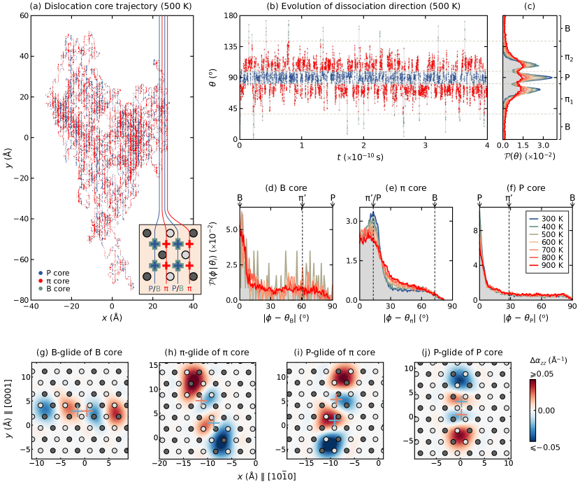
Figure 2: Dislocation core trajectory, dissociation direction and glide direction. (a) The example trajectory of a dislocation core obtained by the MD simulation at $500$ K for 2 ns. The blue, red and green points denote the positions where the core structures are P,   1 0 -.25 1$\pi$ and B, respectively. The inset shows that the P/B cores and the   1 0 -.25 1$\pi$ cores should be distributed on alternating P planes. (b) Temporal evolution of the core dissociation direction $\theta$ extracted from the same MD simulation. (c) Distribution of $\theta$ at the temperature ranging from 300 K to 900 K. The horizontal lines denote the boundaries we defined to distinguish the core structures at 500 K. (d)-(f) Distributions of the deviation of the glide direction $\phi$ away from the dissociation direction $\theta$ for the B,   1 0 -.25 1$\pi$ and P cores. (g)-(i) The differences of the $\alpha_{zz}$ maps at two moments, corresponding to the four dislocation core glide events observed in the simulation. The blue/red “+” symbol indicates the core position in the previous/next moment.

II.2 Dislocation Core Dynamics

We focus on two aspects of dislocation core dynamics: core motion and core structure transitions. The former is analyzed based on the trajectory of the core position (Fig. 2a), while the latter requires recognition of instantaneous core structure. We automated the determination of the core position and the core dissociation direction based on the $\alpha_{zz}$ map. For convenience, we denote the $\alpha_{zz}$-weighted average of any quantity $A$ as

$$\bar{A}=\frac{\iint A(x,y)\alpha_{zz}(x,y)\mathrm{d}x\mathrm{d}y}{\iint\alpha_{zz}(x,y)\mathrm{d}x\mathrm{d}y},$$ (1)

Then, the core position is $\mathbf{r}_{\text{core}}\equiv\left(\bar{x},\bar{y}\right)$; the core positions determined in this manner are indicated by the blue “+” in Figs. 1c-g. Figure 2a shows the core trajectory at $500$ K. From the trajectory, we see that the dislocation random walk is anisotropic. The pattern is elongated along the $y$-axis, suggesting that the dislocation glides on the P plane most frequently.

The glide direction as a function of time $\phi(t)$ is

$$\phi(t)=\arctan\left[\frac{\bar{y}(t+\Delta t)-\bar{y}(t)}{\bar{x}(t+\Delta t)-\bar{x}(t)}\right],$$ (2)

where $\Delta t$ is the time step. The second moment of $\alpha_{zz}$ is the tensor $[C_{ij}]$, where $C_{11}=\overline{x^{2}}$, $C_{22}=\overline{y^{2}}$ and $C_{12}=C_{21}=\overline{xy}$. Suppose that the (normalized) eigenvector of $[C_{ij}]$ corresponding to the maximum eigenvalue is $\mathbf{e}^{*}$. Thus, the core dissociation direction at $t$ is given by

$$\theta(t)=\arctan\left[{e_{y}^{*}(t)}\middle/{e_{x}^{*}(t)}\right].$$ (3)

Figure 2b shows the temporal evolution of the dissociation direction $\theta$ at 500 K and Fig. 2c shows the distribution of the core dissociation direction $\theta$ at different temperatures. The three sharp peaks at $\theta{\simeq}75^{\circ}$, $90^{\circ}$ and $105^{\circ}$ correspond to the $\mbox{\hskip 5.70027pt{1 0 -.25 1}\hbox to0.0pt{\hss\leavevmode\hbox{\set@color$\pi$}}}_{1}$, P and $\mbox{\hskip 5.70027pt{1 0 -.25 1}\hbox to0.0pt{\hss\leavevmode\hbox{\set@color$\pi$}}}_{2}$ cores ($\mbox{\hskip 5.70027pt{1 0 -.25 1}\hbox to0.0pt{\hss\leavevmode\hbox{\set@color$\pi$}}}_{1}$ and $\mbox{\hskip 5.70027pt{1 0 -.25 1}\hbox to0.0pt{\hss\leavevmode\hbox{\set@color$\pi$}}}_{2}$ are both   1 0 -.25 1$\pi$ cores). The peaks for the   1 0 -.25 1$\pi$ cores shift towards $\theta=90^{\circ}$ as temperature increases because the $c/a$ ratio increases with temperature [33]. The peak for the $\mbox{\hskip 5.70027pt{1 0 -.25 1}\hbox to0.0pt{\hss\leavevmode\hbox{\set@color$\pi$}}}^{\prime}$ core, if it existed, would be at $\sim 61^{\circ}$ and $\sim 110^{\circ}$; however, no peaks exist there, implying that the $\mbox{\hskip 5.70027pt{1 0 -.25 1}\hbox to0.0pt{\hss\leavevmode\hbox{\set@color$\pi$}}}^{\prime}$ core may be ignored. At a high temperature (e.g., $900$ K), there are shallow and broad humps at $\theta=0$ or $180^{\circ}$, indicating the existence of the B core at high temperature. The peaks, signaling different cores, broaden with increasing temperature. We set criteria to distinguish the core structures based on the distribution in Fig. 2c. We define the width of the orientation window for the P core as the minima between the P and   1 0 -.25 1$\pi$ cores; i.e., $\sim 90\pm 9^{\circ}$ (the exact position of the minima varies with temperature); see the two dashed lines near $\theta=90^{\circ}$ in Fig. 2b or c. The boundary between the   1 0 -.25 1$\pi$ and B cores is not well defined. Since the probability for $\theta<50^{\circ}$ or $>130^{\circ}$ is almost zero, any quantity evaluated based on the core distribution is insensitive to the choice of this boundary. In practice, we choose the boundary between the   1 0 -.25 1$\pi$ and B cores at the $\theta$ in the middle between $0$ and the $\theta$ for the   1 0 -.25 1$\pi$ core (i.e., the $\theta$ for the second highest peak); see the two dashed lines close to $\theta=90^{\circ}$ in Fig. 2b or c. Using this criterion, we can identify the core structure at any time during the MD simulation. We color each point on the trajectory (at $500$ K) shown in Fig. 2a according to the core structure at each time. We observe that B cores (green points) are rare. The   1 0 -.25 1$\pi$ core (red points) and the P core (blue points) are largely distributed on alternating P planes; this is consistent with the examination of the   1 0 -.25 1$\pi$ and P core positions in the Fig. 2a inset. The Fig. 2a inset shows that ideally the   1 0 -.25 1$\pi$ core is positioned between a dark gray P plane and a light gray P plane, while the P core and B core are between two light gray or two dark gray P planes. Hence, the   1 0 -.25 1$\pi$ and P cores should be distributed on different P planes. Such consistency validates the core structure recognition method.

It is usually assumed that the dislocation core dissociation direction is the same as the dislocation glide direction; this need not be true. To investigate the correlation between the core dissociation direction ($\theta$) and the glide direction ($\phi$), we examine the probability of different glide directions for particular core dissociations (characterized by the dissociation direction $\theta_{i}$ ($i\in\{\mbox{\hskip 5.70027pt{1 0 -.25 1}\hbox to0.0pt{\hss\leavevmode\hbox{\set@color$\pi$}}},\text{P},\text{B}\}$). Figure 2d shows the glide direction distribution for the B core. Most frequently, the B core glides on the B plane (B-glide), corresponding to the peak at $|\theta-\phi_{\text{B}}|=0$. The B-glide of the B core is also seen in the difference between the $\alpha_{zz}$ maps at a pair of times: $\Delta\alpha_{zz}\equiv\alpha_{zz}(t_{2})-\alpha_{zz}(t_{1})$. As shown in Fig. 2g, the alternatively distributed negative and positive $\Delta\alpha_{zz}$ clouds lying on the B plane is a feature of B-glide of B core. The glide direction distribution for the   1 0 -.25 1$\pi$ core is shown Fig. 2e. This distribution exhibits a peak at $|\theta-\phi_{\mbox{\hskip 3.99019pt{1 0 -.25 1}\hbox to0.0pt{\hss\leavevmode\hbox{\set@color$\pi$}}}}|\approx 15^{\circ}$ (at $T=300$ K), where $\theta_{\mbox{\hskip 3.99019pt{1 0 -.25 1}\hbox to0.0pt{\hss\leavevmode\hbox{\set@color$\pi$}}}}\approx 75^{\circ}$. The angle between the $\mbox{\hskip 5.70027pt{1 0 -.25 1}\hbox to0.0pt{\hss\leavevmode\hbox{\set@color$\pi$}}}^{\prime}$ plane (i.e., the $(\bar{1}011)$ plane) and the B plane at 300 K is $\phi=\arctan\left[(2/\sqrt{3})(c/a)\right]\approx 61^{\circ}$; so, if the   1 0 -.25 1$\pi$ core glides on the $\mbox{\hskip 5.70027pt{1 0 -.25 1}\hbox to0.0pt{\hss\leavevmode\hbox{\set@color$\pi$}}}^{\prime}$ plane (  1 0 -.25 1$\pi$-glide), $|\theta-\phi_{\mbox{\hskip 3.99019pt{1 0 -.25 1}\hbox to0.0pt{\hss\leavevmode\hbox{\set@color$\pi$}}}}|\approx 14^{\circ}$. If the   1 0 -.25 1$\pi$ core glides on the P plane (P-glide), $|\theta-\phi_{\mbox{\hskip 3.99019pt{1 0 -.25 1}\hbox to0.0pt{\hss\leavevmode\hbox{\set@color$\pi$}}}}|\approx 15^{\circ}$. This suggests the peak at ${\sim}15^{\circ}$ in Fig. 2e has contributions from both P-glide and   1 0 -.25 1$\pi$-glide. Careful examination, however, shows that P-glide is much more frequent than   1 0 -.25 1$\pi$-glide. The   1 0 -.25 1$\pi$-glide and P-glide of   1 0 -.25 1$\pi$ core can be directly verified by the $\Delta\alpha_{zz}$ maps in Fig. 2h and i. The alternating negative and positive $\Delta\alpha_{zz}$ clouds on the   1 0 -.25 1$\pi$ plane is a feature of   1 0 -.25 1$\pi$-glide of the   1 0 -.25 1$\pi$ core while the off-line distribution of the negative and positive clouds is a feature of P-glide of the   1 0 -.25 1$\pi$ core. The observation that a   1 0 -.25 1$\pi$ core can glide on the P plane contradicts the assumption that the core glide and the core dissociation directions must be the same. Figure 2f shows the glide direction distribution for the P core. Clearly, the P core only glides on P plane. Again, the P-glide of the P core can be verified through considerations of the $\Delta\alpha_{zz}$ clouds distributed along the P plane, as shown in Fig. 2j.

III Model and parameterization of dislocation core dynamics

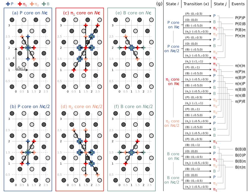
Figure 3: Kinetic events for $\langle\mathbf{a}\rangle$ screw dislocation core dynamics. (a)-(f) All possible events starting from a P core, a   1 0 -.25 1$\pi$ core or a B core. The dark gray and light gray circles denote atoms on successive $(1\bar{2}10)$ planes. The vertical gray solid lines denote a series of $(\bar{2}020)$ planes; the vertical gray dashed lines are offset with respect to the vertical solid lines by $\sqrt{3}a/4$. The horizontal gray solid lines denote a series of $(0001)$ planes ($Nc$ planes); the horizontal gray dashed lines are offset with respect to the horizontal solid lines by $c/2$ (i.e., $Nc/2$ planes). The “$+$” symbols denote dislocation core positions and their colors are consistent with those in the first column of (g). When two “$+$” symbols are located at the same site, we make one larger than the other for clarity. (g) The 1${}^{\text{st}}$ and 3${}^{\text{rd}}$ columns show the starting and ending core structure for one event. The 2${}^{\text{nd}}$nd column shows the core displacements corresponding to the transitions. Some events listed in the 1${}^{\text{st}}$, 2${}^{\text{nd}}$ and 3${}^{\text{rd}}$ columns are connected by the gray lines indicating that they are equivalent in the sense that they have the same energy landscapes. The 4${}^{\text{th}}$ column shows the irreducible events, where $i(\kappa)j$ denotes the transition from an $i$ to $j$ core by glide on plane $\kappa$.

III.1 Kinetic Events

The unit kinetic event during the motion of a dislocation core observed in the MD simulation can be abstracted as a transition. We label the states before and after a transition by $i$ and $j$, respectively, where $i,j\in\text{\{B, $\mbox{\hskip 5.70027pt{1 0 -.25 1}\hbox to0.0pt{\hss\leavevmode\hbox{\set@color$\pi$}}}_{1}$, $\mbox{\hskip 5.70027pt{1 0 -.25 1}\hbox to0.0pt{\hss\leavevmode\hbox{\set@color$\pi$}}}_{2}$, P\}}$. The $\mbox{\hskip 5.70027pt{1 0 -.25 1}\hbox to0.0pt{\hss\leavevmode\hbox{\set@color$\pi$}}}_{1}$ and $\mbox{\hskip 5.70027pt{1 0 -.25 1}\hbox to0.0pt{\hss\leavevmode\hbox{\set@color$\pi$}}}_{2}$ cores denote, respectively, the   1 0 -.25 1$\pi$ cores with the dissociation directions $\theta_{\mbox{\hskip 3.99019pt{1 0 -.25 1}\hbox to0.0pt{\hss\leavevmode\hbox{\set@color$\pi$}}}}\approx 75^{\circ}$ and $105^{\circ}$ (they are symmetry-related). We use $\kappa$ to label the slip plane, i.e., $\kappa\in\text{\{B, $\mathrm{\pi}_{1}$, $\mbox{\hskip 5.70027pt{1 0 -.25 1}\hbox to0.0pt{\hss\leavevmode\hbox{\set@color$\pi$}}}_{2}$, P, 0\}}$, where the $\mbox{\hskip 5.70027pt{1 0 -.25 1}\hbox to0.0pt{\hss\leavevmode\hbox{\set@color$\pi$}}}_{1}$ and $\mbox{\hskip 5.70027pt{1 0 -.25 1}\hbox to0.0pt{\hss\leavevmode\hbox{\set@color$\pi$}}}_{2}$ planes are, respectively, the $\mbox{\hskip 5.70027pt{1 0 -.25 1}\hbox to0.0pt{\hss\leavevmode\hbox{\set@color$\pi$}}}^{\prime}$ planes with the inclination angles $\phi\approx 61^{\circ}$ and $119^{\circ}$, and $\kappa=0$ denotes the transition which does not involve the change in core position. We denote the transition from an $i$ to $j$ core involving glide on the $\kappa$ plane as “$i(\kappa)j$”. An “$i\neq j$” event represents a transition of the core structure, while an “$i=j$” event represents glide of a core with no core structural transition. All possible kinetic events observed in the MD simulations (Fig. 2) are shown schematically in Figs. 3a-f. These events, denoted $i(\kappa)j$, are summarized in Fig. 3g. Some events listed in the 1st, 2nd and 3rd columns are equivalent. The 4th column shows the irreducible events. Note that $\bar{\mbox{\hskip 5.70027pt{1 0 -.25 1}\hbox to0.0pt{\hss\leavevmode\hbox{\set@color$\pi$}}}}$ denotes the core symmetrically related to   1 0 -.25 1$\pi$; e.g., if $\mbox{\hskip 5.70027pt{1 0 -.25 1}\hbox to0.0pt{\hss\leavevmode\hbox{\set@color$\pi$}}}=\mbox{\hskip 5.70027pt{1 0 -.25 1}\hbox to0.0pt{\hss\leavevmode\hbox{\set@color$\pi$}}}_{1}$, then $\bar{\mbox{\hskip 5.70027pt{1 0 -.25 1}\hbox to0.0pt{\hss\leavevmode\hbox{\set@color$\pi$}}}}=\mbox{\hskip 5.70027pt{1 0 -.25 1}\hbox to0.0pt{\hss\leavevmode\hbox{\set@color$\pi$}}}_{2}$.

III.2 Dislocation Core Free Energy

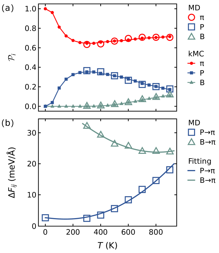
Figure 4: The equilibrium probabilities of core structures and the free energy differences. (a) The probabilities of the   1 0 -.25 1$\pi$ (red circles), P (blue squares) and B (green triangles) cores obtained by the MD simulation (open symbols) and the kMC simulation (solid symbols). (b) The core energy differences, $\Delta F_{\text{P}\mbox{\hskip 3.99019pt{1 0 -.25 1}\hbox to0.0pt{\hss\leavevmode\hbox{\set@color$\pi$}}}}$ (blue squares) and $\Delta F_{\text{B}\mbox{\hskip 3.99019pt{1 0 -.25 1}\hbox to0.0pt{\hss\leavevmode\hbox{\set@color$\pi$}}}}$ (green triangles), obtained from the MD data in (a). The solid lines are the fitting results based on the formula Eq. (5).

From the MD results shown in Fig. 2c, we can extract the equilibrium probabilities $\{\mathcal{P}_{i}\}$ that a core is of type $i$ as a function of temperature. The open symbols in Fig. 4a represent the MD data $\{\mathcal{P}_{i}\}$.   1 0 -.25 1$\pi$ is the most probable core structure at all temperatures,$\mathcal{P}_{\mbox{\hskip 3.99019pt{1 0 -.25 1}\hbox to0.0pt{\hss\leavevmode\hbox{\set@color$\pi$}}}}(T)>0.6$. At $T<300$ K, the B core is not observed in the MD and at $T>300$ K, the B core occurs with very low probability.

In thermal equilibrium at temperature $T$, the probability of finding the $i$ core is well-described by a Boltzmann distribution: $\mathcal{P}_{i}\propto\exp\left(-F_{i}\ell\middle/k_{\text{B}}T\right)$, where $F_{i}$ is the free energy of the $i$ core (energy per length), $\ell$ is the length of the dislocation line, and $k_{\text{B}}$ is the Boltzmann constant. The free energy difference between the $i$ and $j$ cores is related to their probability ratio:

$$\Delta F_{ij}\equiv F_{j}-F_{i}=\frac{k_{\text{B}}T}{\ell}\ln\left(\frac{\mathcal{P}_{i}}{\mathcal{P}_{j}}\right)\text{ with {\hbox{i\neq j}}}.$$ (4)

Since the elastic energy is the same for all core structures, $\Delta F_{ij}$ represents the core energy difference. The core energy difference $\Delta F_{ij}$ at each temperature can be obtained from the MD data $\{\mathcal{P}_{i}\}$ (reported in Fig. 4a) and Eq. (4). Note that although the 10-20 step partial relaxations reduce the potential energy of the system, these energies are not of interest. Rather the partial relaxation simply aids the identification of the inherent core structures. The important energy differences $\Delta F_{ij}$ are determined based on the relative probabilities of different dislocation core structures – which are unaffected by the partial relaxations. The core energy differences, $\Delta F_{\text{P}\mbox{\hskip 3.99019pt{1 0 -.25 1}\hbox to0.0pt{\hss\leavevmode\hbox{\set@color$\pi$}}}}$ and $\Delta F_{\text{B}\mbox{\hskip 3.99019pt{1 0 -.25 1}\hbox to0.0pt{\hss\leavevmode\hbox{\set@color$\pi$}}}}$, are shown as open symbols in Fig. 4b. We can fit the data $\Delta F_{ij}$ with an empirical relationship of the form:

$$\Delta F_{ij}(T)=A+BT\ln T+CT^{2},$$ (5)

where $A$, $B$ and $C$ are parameters. The rationale for the form of this fitting relation is discussed in the SI. For $\Delta F_{\text{P}\mbox{\hskip 3.99019pt{1 0 -.25 1}\hbox to0.0pt{\hss\leavevmode\hbox{\set@color$\pi$}}}}$, $A=E_{\text{P}}-E_{\mbox{\hskip 3.99019pt{1 0 -.25 1}\hbox to0.0pt{\hss\leavevmode\hbox{\set@color$\pi$}}}}=2.6$ meV/Å, where $E_{\text{P}}$ and $E_{\mbox{\hskip 3.99019pt{1 0 -.25 1}\hbox to0.0pt{\hss\leavevmode\hbox{\set@color$\pi$}}}}$ are the energies of the P and   1 0 -.25 1$\pi$ cores at 0 K. The fitted curves are shown as solid lines in Fig. 4b and the parameters are in Table 1.

Table 1: Fit parameters for the free energy difference between cores $i$ and $j$, $\Delta F_{ij}$, as per Eq. (5).

Parameters	$\Delta F_{\text{P}\mbox{\hskip 3.99019pt{1 0 -.25 1}\hbox to0.0pt{\hss\leavevmode\hbox{\set@color$\pi$}}}}$	$\Delta F_{\text{B}\mbox{\hskip 3.99019pt{1 0 -.25 1}\hbox to0.0pt{\hss\leavevmode\hbox{\set@color$\pi$}}}}$
$A$ (meV Å-1)	$2.6$	$41.7\pm 1.25$
$B$ ($10^{-3}$ meV Å-1 K-1)	$-1.65\pm 0.300$	$-7.65\pm 0.833$
$C$ ($10^{-5}$ meV Å-1 K-2)	$3.24\pm 0.266$	$3.59\pm 0.506$

III.3 Core Dynamics Parameterization

The basic kinetic parameters for dislocation core dynamics are the frequencies of all events as a function of temperature. Unfortunately, it is impractical to deduce these frequencies directly from the MD results. Atomic vibrations are inevitable in MD simulations at finite temperatures; removing these by thermal averaging or quenching in order to unambiguously recognize each core event (defined in Fig. 3) requires artificial criteria. Sampling frequency also makes this impractical: if the sampling frequency is too high, the thermal vibration issue will be severe; if it is too low, we will miss some kinetic events. Here, we sidestep the frequency issue, as explained in this section. In short, we fit the MD data using harmonic transition state theory (HTST) with temperature-independent parameters. The general parameterization steps are

• (Prediction) Guess a set of frequencies for all kinetic events $\{\nu_{i(\kappa)j}\}$ at each temperature (see Methods).

• (kMC) At each temperature, perform a kMC simulation (see Methods) with frequencies $\{\nu_{i(\kappa)j}\}$ to compute the core mean squared displacement (MSD), the mean squared angular displacement (MSAD) of the core dissociation direction, and the probability of occurrence of each core structure $\{\mathcal{P}_{i}\}$.

• (Optimization) Optimize $\{\nu_{i(\kappa)j}\}$ such that the MSD, MSAD and $\{\mathcal{P}_{i}\}$ obtained from the kMC are consistent with the MD results at all temperatures (see Methods).

• (Reduction) From $\{\nu_{i(\kappa)j}\}$, extract the fundamental kinetic parameters (attempt frequencies and intrinsic energy barriers) based on HTST.

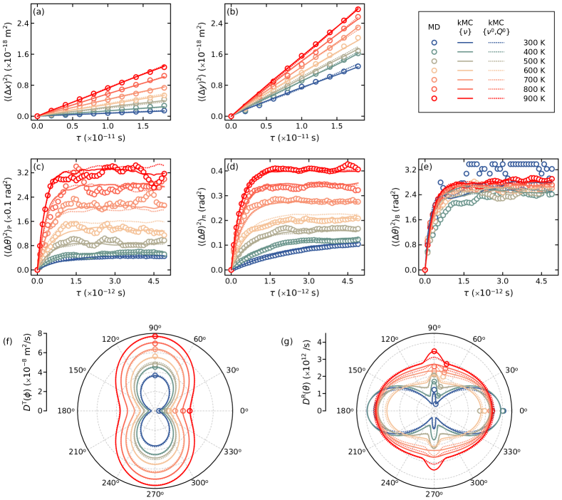
Figure 5: Mean squared displacement and diffusion coefficients. (a) and (b) show the mean squared displacements (MSDs) of a dislocation core in the $x$- and $y$-directions at different temperatures. (c), (d) and (e) show the mean squared angular displacements (MSADs) of a core dissociation direction starting from $\theta_{\text{P}}$, $\theta_{\mbox{\hskip 3.99019pt{1 0 -.25 1}\hbox to0.0pt{\hss\leavevmode\hbox{\set@color$\pi$}}}}$ and $\theta_{\text{B}}$. (f) Translational diffusion coefficient as a function of glide direction, $D^{\text{T}}(\phi)$ at different temperatures. (g) Rotational diffusion coefficient as a function of dissociation direction, $D^{\text{R}}(\theta)$ at different temperatures. In all figures, the circles denote the MD data, the solid lines denote the results of kMC simulations based on the optimized frequencies $\{\nu_{i(\kappa)j}\}$, and the dotted lines denote the results of kMC simulations based on the fitted parameters $\{\nu_{i(\kappa)j}^{0}\}$ and $\{Q_{i(\kappa)j}^{0}\}$.

The mean squared displacement MSD and mean squared angular displacement MSAD (S2 and S3) are defined as follows. At a particular temperature, the mean squared displacement MSD in the $\mathbf{e}_{x}$- and $\mathbf{e}_{y}$-directions are defined as

$$\langle(\Delta x)^{2}\rangle(\tau)=\left\langle[x(t+\tau)-x(t)]^{2}\right\rangle,$$

$$\langle(\Delta y)^{2}\rangle(\tau)=\left\langle[y(t+\tau)-y(t)]^{2}\right\rangle,$$ (6)

where $\langle\cdot\rangle$ denotes the average over $t$. The circles in Figs. 5a and b show the MSDs, $\langle(\Delta x)^{2}\rangle$ and $\langle(\Delta y)^{2}\rangle$, obtained from the MD simulations under different temperatures. We find that core glide along the $\mathbf{e}_{y}$-axis (P plane) is, in general, faster than glide along the $\mathbf{e}_{x}$-axis (B plane). At all temperatures, each MSD is approximately a linear function of $\tau$. The translational diffusion coefficients in the $\mathbf{e}_{x}$- and $\mathbf{e}_{y}$-directions are

$$D_{x}^{\text{T}}=\frac{1}{2}\frac{\mathrm{d}\langle(\Delta x)^{2}\rangle}{\mathrm{d}\tau}\quad\text{and}\quad D_{y}^{\text{T}}=\frac{1}{2}\frac{\mathrm{d}\langle(\Delta y)^{2}\rangle}{\mathrm{d}\tau}.$$ (7)

One goal of optimizing the frequencies $\{\nu_{i(\kappa)j}\}$ is to ensure that the values of $D_{x}^{\text{T}}$ and $D_{y}^{\text{T}}$ from kMC and MD simulations match. The mean squared angular displacement MSAD for core dissociation $i$ is

$$\langle(\Delta\theta)^{2}\rangle_{i}(\tau)=\left\langle[\theta(t+\tau)-\theta(t)]^{2}\right\rangle_{i},$$ (8)

where the subscript “$i$” denotes that in the average $\theta(t=0)=\theta_{i}$, i.e., the dissociation direction of core $i$. The circles in Figs. 5c, d and e show the MSADs, $\langle(\Delta\theta)^{2}\rangle_{\text{P}}$, $\langle(\Delta\theta)^{2}\rangle_{\mbox{\hskip 3.99019pt{1 0 -.25 1}\hbox to0.0pt{\hss\leavevmode\hbox{\set@color$\pi$}}}}$ and $\langle(\Delta\theta)^{2}\rangle_{\text{B}}$, obtained from the MD simulations at different temperatures. The MSAD, at each temperature, is well fitted by the function:

$$\langle(\Delta\theta)^{2}\rangle_{i}(\tau)=2\left(1-e^{-D^{\text{R}}_{i}\tau}\right),$$ (9)

where $D^{\text{R}}_{i}$ ($i=\text{P},\mbox{\hskip 5.70027pt{1 0 -.25 1}\hbox to0.0pt{\hss\leavevmode\hbox{\set@color$\pi$}}},\text{B}$) is the rotational diffusion coefficient about dissociation angle $\theta_{i}$ [34]. In S3, the frequencies $\{\nu_{i(\kappa)j}\}$ are trained for the best match between the core probabilities ($\{\mathcal{P}_{i}\}$), the translational diffusion coefficients ($D^{\text{T}}_{x}$ and $D^{\text{T}}_{y}$) and the rotational diffusion coefficients ($D^{\text{R}}_{\text{P}}$, $D^{\text{R}}_{\mbox{\hskip 3.99019pt{1 0 -.25 1}\hbox to0.0pt{\hss\leavevmode\hbox{\set@color$\pi$}}}}$ and $D^{\text{R}}_{\text{B}}$) obtained by kMC and the MD results. The solid lines in Figs. 5a-c show the MSDs and MSADs obtained from kMC simulations with optimized $\{\nu_{i(\kappa)j}\}$ for different temperatures. The kMC and MD results are in excellent agreement.

We now turn to the parameter space reduction in S4. The frequencies $\{\nu_{i(\kappa)j}\}$ are obtained via S1-3 for the MD simulation temperatures. In principle, dislocation core dynamics at other temperatures may also be obtained from MD simulation at such temperatures and repeating S1-3. The computational resources required for these MD simulations and the optimization process limit the applicability of this approach. We resolve this issue based upon a set of additional assumptions.

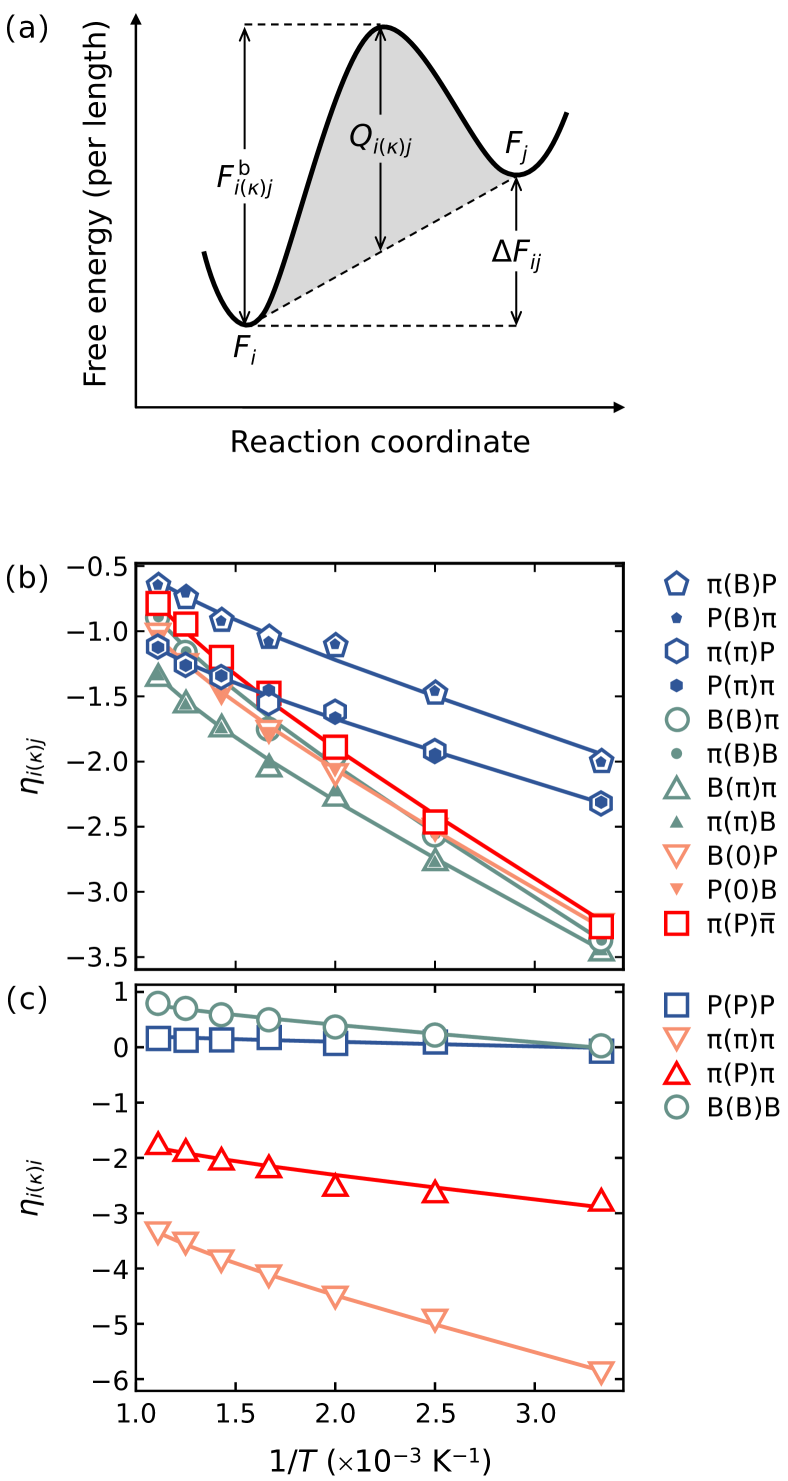
Figure 6: Kinetic model and coefficients. (a) Schematic of the energy landscape for the $i(\kappa)j$ event. $F_{i}$ and $F_{j}$ are the free energies of the $i$ and $j$ cores; $\Delta F_{ij}=F_{j}-F_{i}$ and $\Delta F_{ij}=0$. $F_{i(\kappa)j}^{\text{b}}$ is the total free energy barrier and $Q_{i(\kappa)j}$ is the intrinsic barrier for $i(\kappa)j$. (b) $\eta_{i(\kappa)j}$ (Eq. (III.3)) vs. inverse temperature. (c) $\eta_{i(\kappa)i}$ (Eq. (III.3) for glide events) vs. the inverse temperature. In (b) and (c), symbols and solid lines denote MD data and fitting results (Eqs. (III.3) and (13)).

Consider the schematic energy landscape for a kinetic event $i(\kappa)j$ in Fig. 6a. Two local minima correspond to the $i$ and $j$ core free energies, $F_{i}$ and $F_{j}$. The core energy difference is $\Delta F_{ij}$ (Eq. (4)); for a core glide event, $\Delta F_{ii}=0$. The total free energy barrier for $i(\kappa)j$ is denoted $F_{i(\kappa)j}^{\text{b}}$. The intrinsic free energy barrier for $i(\kappa)j$ is $Q_{i(\kappa)j}$ and, in principle, $Q_{i(\kappa)j}=Q_{j(\kappa)i}$. The total free energy barrier is commonly approximated as

$$F_{i(\kappa)j}^{\text{b}}=Q_{i(\kappa)j}+\Delta F_{ij}/2,$$ (10)

where the factor $1/2$ is valid when $\Delta F_{ij}\ll Q_{i(\kappa)j}$ [26]. While other reasonable proposals for $F_{i(\kappa)j}^{\text{b}}$ are possible, our fitting results, below, suggest that Eq. (10) reproduces the MD results.

The frequency of event $i(\kappa)j$ can be expressed as

$$\nu_{i(\kappa)j}=\nu_{i(\kappa)j}^{0}\exp\left(-\frac{F_{i(\kappa)j}^{\text{b}}\ell}{k_{\text{B}}T}\right)$$ (11)

based on HTST [35, 36], where $\nu_{i(\kappa)j}^{0}$ is an attempt frequency that includes the effect of barrier recrossing. Equation (11) can be rewritten as

$$\eta_{i(\kappa)j}(T^{-1}) \equiv\ln\left(\nu_{i(\kappa)j}\sqrt{\mathcal{P}_{i}/\mathcal{P}_{j}}\right)$$

$$=\ln\nu_{i(\kappa)j}^{0}-\frac{Q_{i(\kappa)j}\ell}{k_{\text{B}}T}.$$ (12)

This shows that $\eta_{i(\kappa)j}$ is a function of the inverse temperature $T^{-1}$. If $\{\nu_{i(\kappa)j}^{0}\}$ and $\{Q_{i(\kappa)j}\}$ are constant with respect to temperature, they can be obtained by linear fitting. However, we find that the fitting quality is improved by allowing the intrinsic free energy barrier to be temperature-dependent and of the form:

$$Q_{i(\kappa)j}=Q_{i(\kappa)j}^{0}\left[1-\left(\frac{T}{T_{0}}\right)^{q}\right],$$ (13)

where $Q_{i(\kappa)j}^{0}$ is the intrinsic barrier at 0 K, $T_{0}=1250$ K is the HCP-BCC transition temperature for this DP potential [33], and we assign $q=3$ to give best fit to all the data. Equation (13) is proposed based on the observations that (i) the free energy barrier decrease with increasing temperature and (ii) when the HCP phase becomes unstable/metastable, the transition between the core structures is barrierless. In this way, the kinetic parameters can be fitted to the MD data; i.e., $\{\nu_{i(\kappa)j}^{0}\}$ and $\{Q_{i(\kappa)j}^{0}\}$.

Figures 6b and c show the fitting results for Eqs. (III.3) and (13) (symbols/lines are the MD data/fits). As expected, the $i(\kappa)j$ and $j(\kappa)i$ data coincide. Among the transition events (Fig. 6b), the transitions between P and   1 0 -.25 1$\pi$ cores are the most frequent and associated with the lowest energy barriers. As expected, direct transitions between P and B cores are rare. Among the glide events (Fig. 6c), the glide on B plane is associated with the lowest barrier. But glide on B plane is rare since the probability of the B core is very low (Fig. 4a). Pyramidal glide (via $\mbox{\hskip 5.70027pt{1 0 -.25 1}\hbox to0.0pt{\hss\leavevmode\hbox{\set@color$\pi$}}}(\mbox{\hskip 5.70027pt{1 0 -.25 1}\hbox to0.0pt{\hss\leavevmode\hbox{\set@color$\pi$}}})\mbox{\hskip 5.70027pt{1 0 -.25 1}\hbox to0.0pt{\hss\leavevmode\hbox{\set@color$\pi$}}}$) is much less frequent and associated with a much higher barrier than prismatic glide (via P(P)P). This means that pyramidal glide is rarer than prismatic glide; in qualitative agreement with the DFT 0 K glide barriers [10] (DFT predicts the Peierls barrier for P(P)P glide and $\pi(\pi)\pi$ glide as 11.4 meV Å^-1 and 0.4 meV Å^-1, while the values from our simulations are 14.1 meV Å^-1 and 1.14 meV Å^-1).

Table 2: The kinetic parameters determined by fitting to the MD data for the core transition events and glide events. $\nu_{ik}^{0}$ is the attempt frequency in Eq. (III.3). $Q_{ik}^{0}$ is the intrinsic 0 K energy barrier in Eq. (13).

Events $i(\kappa)j$	$Q_{i(\kappa)j}^{0}$ (meV Å-1)	$\nu_{i(\kappa)j}^{0}$ (ps-1)
$i\neq j$: core transition
B(B)  1 0 -.25 1$\pi$	$13.9\pm 0.444$	$0.782\pm 0.0450$
B(0)P	$12.6\pm 0.172$	$0.636\pm 0.0141$
1 0 -.25 1$\pi$(B)P	$7.47\pm 0.447$	$0.769\pm 0.0445$
1 0 -.25 1$\pi$(P)$\bar{\mbox{\hskip 5.70027pt{1 0 -.25 1}\hbox to0.0pt{\hss\leavevmode\hbox{\set@color$\pi$}}}}$	$13.7\pm 0.209$	$0.871\pm 0.0236$
1 0 -.25 1$\pi$(  1 0 -.25 1$\pi$)P	$6.69\pm 0.125$	$0.442\pm 0.00718$
B(  1 0 -.25 1$\pi$)  1 0 -.25 1$\pi$	$11.8\pm 0.221$	$0.457\pm 0.0131$
$i=j$: core glide
B(B)B	$4.33\pm 0.237$	$2.61\pm 0.0800$
1 0 -.25 1$\pi$(  1 0 -.25 1$\pi$)  1 0 -.25 1$\pi$	$14.1\pm 0.315$	$0.0689\pm 0.00281$
1 0 -.25 1$\pi$(P)  1 0 -.25 1$\pi$	$6.06\pm 0.760$	$0.216\pm 0.0213$
P(P)P	$1.14\pm 0.295$	$1.18\pm 0.0488$

IV Kinetic Monte Carlo simulation results

The model and parameterization of the core dynamics described are the key for understanding and predicting dislocation dynamics. Here, we apply this model to $\langle\mathbf{a}\rangle$ screw dislocation dynamics in Ti via kinetic Monte Carlo (kMC) simulations (see Methods). The only modification is that the kinetic event frequencies $\{\nu_{i(\kappa)j}\}$ are determined through Eqs. (10), (11) and (13).

IV.1 Random Walk of a Dislocation Core

The equilibrium core structure probabilities $\{\mathcal{P}_{i}\}$ were computed via kMC and compared with those obtained from MD, as shown in Fig. 4a. At temperatures $\geq 300$ K, the kMC results show excellent agreement with MD. $\mathcal{P}_{\mbox{\hskip 3.99019pt{1 0 -.25 1}\hbox to0.0pt{\hss\leavevmode\hbox{\set@color$\pi$}}}}$ and $\mathcal{P}_{\mathrm{P}}$ exhibit a minimum and maximum near 300 K. Beyond this temperature both $\mathcal{P}_{\mbox{\hskip 3.99019pt{1 0 -.25 1}\hbox to0.0pt{\hss\leavevmode\hbox{\set@color$\pi$}}}}$ and $\mathcal{P}_{\mathrm{B}}$ increase, while $\mathcal{P}_{\mathrm{P}}$ decreases with temperature $T$. $\mathcal{P}_{\mathrm{P}}$ and $\mathcal{P}_{\mathrm{B}}$ are approximately equal near 0 and 900 K. No MD is available below 300 K where it is difficult to obtain valid statistics; here, we only show kMC data from Eq. (5). At 0 K, based on the fact that   1 0 -.25 1$\pi$ core is energetically favorable, $\mathcal{P}_{\mbox{\hskip 3.99019pt{1 0 -.25 1}\hbox to0.0pt{\hss\leavevmode\hbox{\set@color$\pi$}}}}$ should be 1 and $\mathcal{P}_{\mathrm{P}}$ and $\mathcal{P}_{\mathrm{B}}$ should be 0. $\mathcal{P}_{\mathrm{B}}\approx 0$ for $T\leq 300$ K, which is consistent with the MD observation that the B core is unstable.

The MSDs and MSADs computed via MD and kMC simulations are compared in Fig. 5a-e. In general, the kMC simulations reproduce the MD results well, except for the MSADs corresponding to core dissociation starting from $\theta_{\text{B}}$ at low temperatures (Fig. 5e) (this is associated with limited sampling of the B core in the MD simulations). Due to larger accessible timescale in kMC compared with MD, the kMC simulations provide smooth curves at low computational cost (compared with MD). The glide-direction dependent translational diffusion coefficient can be constructed as

$$D^{\mathrm{T}}(\phi)=D^{\mathrm{T}}_{x}\cos^{2}\phi+D^{\mathrm{T}}_{y}\sin^{2}\phi;$$ (14)

see Fig. 5f. $D^{\mathrm{T}}(\phi)$ is elongated in the $\mathbf{e}_{y}$-direction, indicating that a dislocation core moves fast along the P plane and slowly along the B plane; this is consistent with the MD trajectories in Fig. 2a. The dissociation-angle-dependent rotational diffusion coefficient can be constructed as

$$D^{\mathrm{R}}(\theta)=D^{\mathrm{R}}_{i}\cos^{2}\left(\frac{\pi}{2}\frac{\theta-\theta_{i}}{\theta_{j}-\theta_{i}}\right)+D^{\mathrm{R}}_{j}\sin^{2}\left(\frac{\pi}{2}\frac{\theta-\theta_{i}}{\theta_{j}-\theta_{i}}\right),$$ (15)

where $(i,j)=(\text{B},\mbox{\hskip 5.70027pt{1 0 -.25 1}\hbox to0.0pt{\hss\leavevmode\hbox{\set@color$\pi$}}})$ or $(\mbox{\hskip 5.70027pt{1 0 -.25 1}\hbox to0.0pt{\hss\leavevmode\hbox{\set@color$\pi$}}},\text{P})$; see Fig. 5g. $D^{\text{R}}(\theta)$ measures the rotation rate for cores initially oriented at angle $\theta$. Figure 5g shows that $D^{\text{R}}(\theta)$ is highly anisotropic at low temperatures and becomes more isotropic as temperature increases. At all temperatures (except for 900 K), $D^{\text{R}}$ is maximum at $\theta=0$ which corresponds to the B core. This is consistent with the fact that B core is not energetically favorable and tends to transform into other cores. $D^{\text{R}}$ is a minimum at ${\sim}\theta=75^{\circ}$; corresponding to the $\pi$ core. This indicates that the most stable core is $\pi$.

IV.2 Stress-Driven Dislocation Motion

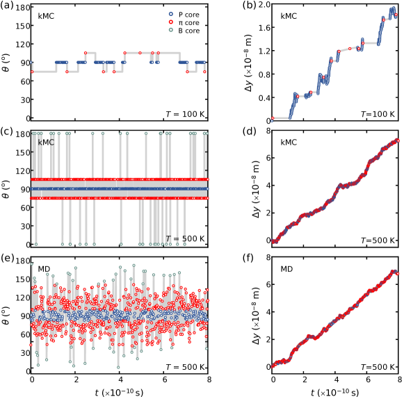
Figure 7: Temporal evolutions of the dislocation core dissociation angle ($\theta$) and the core displacement along P plane ($\Delta y$). (a) and (b) The core trajectories under $\sigma_{yz}=$10 MPa at 100 K predicted by kMC. (c) and (d) The core trajectories under $\sigma_{yz}=$60 MPa at 500 K predicted by kMC. (e) and (f) The core trajectories under $\sigma_{yz}=$60 MPa at 500 K obtained by MD. In all figures, blue, red and green circles label the P,   1 0 -.25 1$\pi$ and B cores, respectively.

The kMC model is sufficiently flexible to simulate dislocation dynamics under an externally applied stress. We apply the approach developed by Ivanov and Mishin [37].

The major assumption is that the applied stress influences the dislocation glide barrier through the resolved shear stress (RSS), but not the energy barrier for the core transition itself. Hence, this model does not fully capture the non-Schmid effect [38, 39, 40, 41] (see below).

We assume that the free energy landscape for $i$ core glide on the $\kappa$ plane has the form of $F_{i(\kappa)i}(r)=(Q_{i(\kappa)i}/2)[1-\cos(2\pi r/L_{i(\kappa)i})]$, where $r$ is a slip distance, $Q_{i(\kappa)i}$ is the glide barrier (Eq. (13)) and $L_{i(\kappa)i}$ is a lattice period in the slip direction on the $\kappa$ plane. Applying an external stress $\bm{\sigma}$ creates Gibbs free energy landscape $G_{i(\kappa)i}(r)=F_{i(\kappa)i}(r)-f_{\kappa}r$, where $f_{\kappa}$ is the Peach-Koehler (PK) force: $f_{\kappa}=(\bm{\sigma}\mathbf{b})\times\bm{\xi}\cdot\mathbf{s}_{\kappa}=\tau_{\kappa}b$. With our sample geometry, Fig. 1a, $\bm{\xi}=\mathbf{e}_{z}$ is the line direction, $\mathbf{b}=b\mathbf{e}_{z}$ is the Burgers vector, $\mathbf{s}_{\kappa}=\cos\phi_{\kappa}\mathbf{e}_{x}+\sin\phi_{\kappa}\mathbf{e}_{y}$ is the slip direction on the $\kappa$ plane with inclination angle $\phi_{\kappa}$, and $\tau_{\kappa}\equiv-\sigma_{xz}\sin\phi_{\kappa}+\sigma_{yz}\cos\phi_{\kappa}$ is the RSS on the $\kappa$ plane. Then, the Gibbs free energy barrier for the forward/backward glide is

$$G_{i(\kappa)i}^{\text{b}\pm} =Q_{i(\kappa)i}\Bigg{[}\sqrt{1-\left(\frac{\tau_{\kappa}}{\tau_{i(\kappa)i}^{0}}\right)^{2}}$$

$$\mp\frac{\pi\tau_{\kappa}}{2\tau_{i(\kappa)i}^{0}}\left(1\mp\frac{2}{\pi}\arcsin\frac{\tau_{\kappa}}{\tau_{i(\kappa)i}^{0}}\right)\Bigg{]},$$ (16)

where $\tau_{i(\kappa)i}^{0}\equiv\pi Q_{i(\kappa)i}/(L_{i(\kappa)i}b)$. The frequency of forward/backward glide event $i(\kappa)i$, $\nu_{i(\kappa)i}^{\pm}$, is obtained from Eq. (11) with $F_{i(\kappa)i}^{\text{b}}$ replaced by $G_{i(\kappa)i}^{\text{b}\pm}$; $\nu_{i(\kappa)i}=\nu_{i(\kappa)i}^{+}-\nu_{i(\kappa)i}^{-}$. The detailed explanation of Eq. (IV.2) can be found in Ref. [37]. With this frequency as input, we perform kMC simulations of dislocation motion under different stresses $\bm{\sigma}$ (see Methods).

The kMC simulations show a locking-unlocking type of dislocation motion at low temperatures. Figures 7a and b show the temporal evolution of the dislocation core dissociation angle, $\theta$, and the core displacement in the $\mathbf{e}_{y}$-direction (P plane), $\Delta y$, at $T=100$ K under shear stress $\sigma_{yz}=10$ MPa. When the dislocation core has a P core (blue circles), $\Delta y$ increases quickly; i.e., P-glide is fast. On transformation to a   1 0 -.25 1$\pi$ core (red circles), the dislocation pauses while “waiting” to transform back to a P core (Fig. 7a) upon which glide restarts on the P plane (Fig. 7b). Hence, the   1 0 -.25 1$\pi$ core is “locked” (does not glide) and the P core is “unlocked” (glides easily).

The “locking” period predicted by kMC ($\sim 10^{-10}$ s) is much smaller than that observed in in situ TEM straining experiments ($\sim 8$ s) [10]. There are two possible sources for this discrepancy. The TEM specimen is a thin foil, the free surfaces of which could provide strong drag on the dislocation. We have performed additional MD simulations, involving a dislocation line threaded at two free surfaces, to examine the drag effect (see SI for the simulation settings and results). The simulation results confirm that the free surfaces significantly reduce the dislocation mobility by imposing severe restrictions on core transitions. Second, our kMC simulations only study the motion of a short dislocation segment, rather than a long dislocation line. The differences in dislocation mobility between our work and TEM observations are attributed to the differences in dislocation line length. The motion of long dislocation lines involves collective motion of many dislocation segments, thus a higher free energy barrier should be overcome during the glide process. Moreover, long dislocations may migrate via kink pair nucleation and propagation, which necessitate inclusion of kink formation and migration energy barriers in estimation of dislocation mobility. Multiple core structures will likely be found on a long dislocation line. The interaction between these different core structures may also lower the dislocation mobility. This, coupled with the free surface restraint on core transitions (see SI) explains why short dislocation segments are more mobile than long dislocation lines in TEM observations.

To validate our kMC results, we simulated dislocation core motion at high temperature (500 K) at a high shear stress ($\sigma_{yz}=60$ MPa) by both kMC and DP-based MD (note that the MD time scale only allows the study of fast dynamics which can be achieved at high temperatures and high driving forces). Figures 7c and d show the evolution of $\theta$ and $\Delta y$ obtained through kMC simulations, while Fig. 7e and f show the same quantities under the same conditions from MD. The kMC and MD results are consistent. At this high temperature, the locking-unlocking mechanism is not easily seen, although it effectively lowers the core velocity along the P plane.

IV.3 Dislocation Mobility

A shear stress $\bm{\sigma}=\sigma_{xz}(\mathbf{e}_{x}\otimes\mathbf{e}_{z}+\mathbf{e}_{z}\otimes\mathbf{e}_{x})$ creates a PK force on the screw dislocation $\mathbf{f}=\sigma_{xz}b\mathbf{e}_{x}$; the dislocation moves, on average, in the $\mathbf{e}_{x}$-direction, i.e., on the B plane. We found that the dislocation velocity on the B plane, $v_{\text{B}}$, is a linear function of $\sigma_{xz}$ (see the kMC and MD data in SI). The dislocation mobility on the B plane is $M_{\text{B}}=v_{\text{B}}/(\sigma_{xz}b)$. Alternatively, we may drive the dislocation motion on the P plane via shear stress $\bm{\sigma}=\sigma_{yz}(\mathbf{e}_{y}\otimes\mathbf{e}_{z}+\mathbf{e}_{z}\otimes\mathbf{e}_{y})$ to obtain $M_{\text{P}}=v_{\text{P}}/(\sigma_{yz}b)$. If the energy barrier for a core transition or glide event is large, the intrinsic free energy barrier, $Q_{i(\kappa)j}$, is the Peierls barrier and the dislocation motion is thermally activated. On the other hand, if it is small, $Q_{i(\kappa)j}$ cannot be interpreted as Peierls barrier; it is simply a parameter in the model which reproduces the frequencies obtained from MD. Dislocation mobility in the case of small energy barrier is phonon damping-controlled such that the viscous drag coefficient is $M_{\text{B}}^{-1}$ or $M_{\text{P}}^{-1}$ [42]. Phonon damping is not explicitly modeled in kMC; rather it is captured through the parameterization of the frequency obtained from MD (similar to the method reported in Ref. [28]).

The temperature-dependencies of $M_{\mathrm{B}}$ and $M_{\mathrm{P}}$ are shown in Fig. 8. $M_{\text{B}}$ is much lower than $M_{\text{P}}$ at all temperatures, as suggested by Fig. 5f (where the dislocation core diffusion coefficient is a minimum/maximum at $\phi=0/90^{\circ}$. As shown in Fig. 8a and its inset, $M_{\text{B}}$ increases with temperature monotonically while $M_{\text{P}}$ exhibits a maximum at $T=300$ K (indicated by the dash-dotted line). The decrease of $M_{\text{P}}$ and increase of $M_{\text{B}}$ above 300 K is consistent with the MD results, i.e., the crosses in Fig. 8a inset. MD simulations from the literature [43, 44, 45, 46] always show that the dislocation mobility decreases (or equivalently, the viscous drag coefficient increases) with increasing temperature. However, we note that MD results at low temperatures do not exist, since MD timescales do not suffice. The decrease in mobility (increase in viscous drag coefficient) at high temperature is usually interpreted as a phonon drag/damping effect. However, our kMC results suggest that glide on the P plane is also effectively damped by dislocation core transitions to B core. With increasing temperature, the B core is increasingly stable (Fig. 4a) such that the transition rate from the   1 0 -.25 1$\pi$ core to the B core increases (Fig. 6b), leading to B-glide which contributes to zero motion on the P plane.

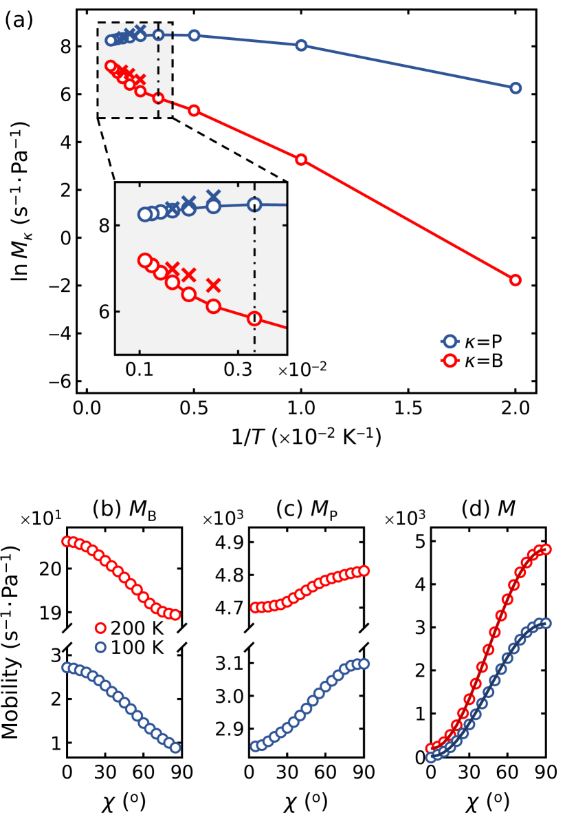
Figure 8: (a) Arrhenius plot of dislocation mobilities on the P plane for $\sigma_{yz}$ (blue) and B plane for $\sigma_{xz}$ (red). The circles and crosses are, respectively, the kMC and MD data. The dash-dotted line indicates $T=300$ K. (c) and (d) The mobilities on the B and P planes ($M_{\text{B}}$ and $M_{\text{P}}$) as a function of PK force direction $\chi$. (d) The scalar dislocation mobility as a function of $\chi$. The symbols are kMC data while the solid lines are fits to Eq. (IV.3). In (b)-(d) the blue and red circles correspond to 100 K and 200 K.

We also investigated the effect of shear stress orientation and dislocation mobility anisotropy. A PK force may be applied in different directions, by choice of the relative magnitudes of $\sigma_{xz}$ and $\sigma_{yz}$; i.e., $\mathbf{f}=\sigma_{xz}b\mathbf{e}_{x}+\sigma_{yz}b\mathbf{e}_{y}$. The orientation angle (maximum resolved shear stress plane, MRSSP) is $\chi=\arctan(f_{\text{P}}/f_{\text{B}})=\arctan(\sigma_{yz}/\sigma_{xz})$, where $f_{\mathrm{P}}$ and $f_{\mathrm{B}}$ are the PK forces resolved on to the P and B planes. We calculated $M_{\text{P}}$ and $M_{\text{B}}$ for various values of $\chi$ under 100 K and 200 K; the results are shown in Figs. 7g and h. There is no surprise that $M_{\mathrm{B}}$ decreases and $M_{\text{P}}$ increases as $\chi$ increases from 0 to 90^∘, and the high-temperature mobilities are higher than the low-temperature counterparts. The dislocation mobility can be generalized to a tensor, $\mathbf{M}$, defined by the relationship: $\mathbf{v}=\mathbf{M}\mathbf{f}$. The dislocation glide velocity component parallel to the PK force is $v=\hat{\mathbf{f}}\cdot\mathbf{v}=(\hat{\mathbf{f}}\cdot\mathbf{M}\hat{\mathbf{f}})f=Mf$, where $\hat{\mathbf{f}}=(\cos\chi,\sin\chi)^{T}$ is the direction of PK force and the scalar dislocation mobility is

$$M(\chi)\equiv\hat{\mathbf{f}}\cdot\mathbf{M}\hat{\mathbf{f}}$$

$$=M_{11}\cos^{2}\chi+M_{22}\sin^{2}\chi+2M_{12}\sin\chi\cos\chi,$$ (17)

where $M_{\text{P}}=M(0)=M_{11}$ and $M_{\text{B}}=M(90^{\circ})=M_{22}$. We measured the velocity component parallel to the PK force ($v$) and calculated the scalar mobility ($M=v/f$) as a function of $\chi$; see Fig. 8d. Next, we extracted $M_{ij}$ by fitting $M$ vs. $\chi$ to Eq. (IV.3); see the solid lines in Fig. 8d. We find that $M_{11}=M_{\text{B}}(\chi=0)$, $M_{22}=M_{\text{P}}(\chi=90^{\circ})$ and $M_{12}$ is negligibly small in comparison with $M_{11}$ and $M_{22}$. Since $M_{11}\neq M_{22}$, the dislocation velocity $\mathbf{v}$ is, in general, not in the same direction as the PK force $\mathbf{f}$. The off-diagonal component $M_{12}$ relates to how the PK force, resolved on B/P plane, influences dislocation glide on the P/B plane – this is a non-Schmid effect [38]. $M_{12}\approx 0$ indicates that dislocation glide is well-described by the Schmid law in our kMC model.

IV.4 Limitations

IV.4.1 Non-Schmid effects

The glide probabilities are deduced from dislocation random walk (i.e., with no driving force), from which we extracted the intrinsic glide barriers. Applied stress does not change the intrinsic glide barriers, but rather biases the glide barriers according to Eq. (IV.2). The Schmid effect is naturally included in this model, since the glide barrier will be lowered the most along the plane where the resolved shear stress is the maximum.

We do not investigate non-Schmid effects in this study as this is not an intrinsic property. To capture non-Schmid effects generally necessitates determination of how the entire 6-dimensional stress tensor alters the glide barrier. More specifically, it is possible to repeat our sampling and analysis presented in this work as a function of stress normal to the P-plane, $\pi$-plane or B-plane. This is beyond the scope of this study.

IV.4.2 Long dislocation lines

The present simulations focused mainly on understanding the effect of intrinsic dislocation core properties/behavior on dislocation motion. Hence, all simulations were performed to short dislocation segments. While this helps obtain fundamental, intrinsic core behavior, it does not account for all aspects of dislocation dynamics. Nevertheless, it is of practical interest to understand how a long, screw dislocation line moves in $\alpha$-Ti. The mechanism of the motion of a long dislocation line is associated with nucleation and propagation of kinks. Both kink nucleation and propagation necessarily involve the advance of local short dislocation segments. In this sense, the core properties extracted in this paper serve as essential input to such higher-level, long dislocation line models/simulations.

A serious treatment of long dislocations should be multiscale. Even the extant long ($32b$) dislocation MD simulations (e.g., see Ref. [14]) have not resolved the size effect issue. At a high temperature ($k_{\text{B}}T$ exceeds the kink energy), a dislocation line will likely undergo thermal roughening (i.e., the fluctuation amplitude of a dislocation line scales with the size of system) [47]. If so, the size effect cannot be overcome by any finite length scale MD simulation. A possible strategy is to incorporate the intrinsic dislocation core properties as inputs for a multiscale method, such as kMC, rather than to simulate a long dislocation directly by MD. To do this, additional information is required (e.g., double kink formation and migration barriers or migration velocities); these may be obtained either directly from MD simulations or by derivation. For example, Edagawa’s line tension model [48] provides a reasonable description of variations of the double-kink nucleation energy, which can also be directly obtained from atomistic simulation by modeling a kink structure [49]. The kink migration barrier may be obtained from atomistic simulation for determination of Peierls barrier [49]. If the kink migration barrier is much lower than the screw dislocation migration barrier, the kink velocity can be used in place of the migration barrier in kMC simulations [27]. All above allow for the effective parameterization of long dislocations for kMC simulations (e.g., those proposed by Cai and collaborators [27, 23]) of long dislocations in complex materials.

V Conclusion

We have studied the finite-temperature core structures of $\langle\mathbf{a}\rangle$ screw dislocations in HCP Ti, through a multi-scale framework. First, we characterize atomic interactions in Ti based upon machine learning, Deep Potentials (DP), which reproduce the stable/metastable dislocation core structures found via quantum mechanical, DFT calculations. DP was employed in molecular dynamics (MD) simulations of screw dislocation core structure at finite temperatures. MD provides the statistics of directional dislocation core dissociation (  1 0 -.25 1$\pi$, P and B cores) and directional core glide (  1 0 -.25 1$\pi$-, P- and B-glide). We found that the   1 0 -.25 1$\pi$ core is stable and the P core is metastable, consistent with 0 K DFT results, while the B core is metastable above 300 K. Contrary to common understanding, the glide direction need not align with the core dissociation direction; e.g.,   1 0 -.25 1$\pi$ core can glide on the P plane.

The MD observations allow us to identify all important unit kinetic events associated with dislocation core motion. The events were categorized as either core transition (change in the dissociation direction) or core glide events (unit displacement along a slip plane). These events were incorporated into a kinetic model and that was parameterized through the MD data. The machine learning-based fitting procedure ensures that the frequency of each core structure and the translational and rotational diffusion coefficients produced by a kinetic Monte Carlo (kMC) simulation implementation of the model are consistent with MD data. We found that P core glide on the P plane event has the lowest core glide barrier, the transition between P and   1 0 -.25 1$\pi$ cores has the lowest barrier among all core transition events, and the glide of the   1 0 -.25 1$\pi$ core (on any plane) is very difficult.

With the parameters (barriers and frequencies) obtained by fitting, the proposed kMC simulation procedure is applicable to dislocation core dynamics at any temperature and applied stress. The dislocation will undergo a random walk (diffusion) in the absence of an applied stress; long-time dislocation core trajectories provide anisotropic translational and rotational diffusion coefficients. The former indicates that dislocation motion on the P plane is fastest and motion on the B plane is slowest. This implies that the   1 0 -.25 1$\pi$ core is difficult to rotate and is stable while rotation away from the B core is fast. Under an applied stress, dislocation motion occurs through a locking-unlocking process at low temperatures, consistent with experimental observations. The locking behavior originates from the high energy barrier associated with   1 0 -.25 1$\pi$ core glide. Application of different stress states yields that the motion of $\langle\mathbf{a}\rangle$ screw core in Ti is anisotropic. The temperature dependence of this anisotropy is consistent with the (limited) MD predictions.

This work demonstrates that the intrinsic dynamic behavior of dislocations cannot be described based upon studies of 0 K dislocation core structures alone. Rather, statistical examination of the finite-temperature core structures is essential to determine, not only, the finite-temperature stability of different core structures, but also the kinetic properties of dislocation motion and core structure transitions. The kinetic model and parameters obtained in this work provide the necessary inputs for the higher-level approaches, such as kMC simulation of long dislocation line (for which kink nucleation and propagation are considered) and discrete dislocation dynamics. While the present study focuses on screw dislocation motion in Ti, the method described here is applicable to all dislocation types, at any temperature and stress state, in both simple (cubic) and complex (non-cubic) crystalline materials.

Methods

MD Simulations

The simulations employ a Deep Potential (DP) trained using DFT results for perfect crystals and defects in the $\alpha$, $\beta$ and $\omega$ phases of Ti [33]. This DP successfully reproduces the 0 K core structures of the $\langle\mathbf{a}\rangle$ screw dislocations in Ti as predicted by DFT [33].

The MD simulation cell geometry is shown in Fig. 1a. An HCP $\alpha$-Ti single crystal cylinder is constructed such that the $[1\bar{2}10]$ is parallel to the cylinder axis; the Cartesian coordinate system employed has $\mathbf{e}_{x}\parallel[10\bar{1}0]$, $\mathbf{e}_{y}\parallel[0001]$ and $\mathbf{e}_{z}\parallel[1\bar{2}10]$. The simulation cell is periodic along the $\mathbf{e}_{z}$-axis. An $\langle\mathbf{a}\rangle$ screw dislocation, with both Burgers vector and line direction parallel to $\mathbf{e}_{z}$, is introduced in the center of the cylinder by displacing the atoms according to the anisotropic elasticity solution (lattice parameters and elastic constants for this potential as a function of temperature). The configuration is equilibrated at different temperatures in an $NVT$ ensemble. The interactions between atoms in Region I (see Fig. 1a) are described by the DP for Ti. The atoms in Region II are described as an Einstein crystal, i.e., the atoms are tethered at the coordinates of the as-constructed (with anisotropic elastic displacements of atoms from their perfect crystal locations) configuration by harmonic springs, to avoid the free surface of Region II which will apply image force on the dislocation core. The interface between Region I and II has negligible effect on the simulation results. Details can be found in the SI. The spring constant is determined as $3k_{\text{B}}T/\langle(\Delta\mathbf{r}_{\text{atom}})^{2}\rangle$, where $k_{\text{B}}$ is the Boltzmann constant, $T$ is the absolute temperature and $\langle(\Delta\mathbf{r}_{\text{atom}})^{2}\rangle$ is the mean squared displacement of atoms at the temperature $T$. The radius of Region I is $\sim 160$ Å, the width of Region II is $\sim 18$ Å, and the dislocation line length is $\sim 6$ Å. The whole system contains $\sim 33,000$ atoms; i.e., large enough that Region II and the interface between Region I and II have little influence on the random walk of the dislocation core about the center of Region I; see SI for details. The cylindrical sample containing a dislocation was equilibrated for 2 ns at each temperature. All MD simulations were performed using lammps [50].

The dislocation configurations were thermally equilibrated at temperatures 300-900 K (well below the HCP-BCC transition temperature, 1250 K). The atomic configuration was recorded every 50 fs. Energy minimization for 10-20 steps (by conjugate gradient with line-search step size 0.01 Å) was conducted for each of these atomic configurations to remove thermal vibration in order to clearly visualize/analyze the atomic structure [23]. Such energy minimization has little effect on the dislocation core distribution (for details, see SI).

Nye tensor parameters

The Nye tensors are visualized with perfect crystals as references. Two key parameters govern the presentation of the Nye tensor plot are the cutoff distance for constructing a neighbor list and the maximum angle ($\Theta$) employed to identify matches between $\mathbf{p}$ and $\mathbf{q}$ vectors – here, $\mathbf{p}$ and $\mathbf{q}$ denote the radial distance vectors between each atom and its neighbors in the reference and current systems, respectively. In our investigation, we have chosen a cutoff distance that corresponds to $1.3$ times the equilibrium lattice constant at the temperature of interest. We set $\Theta$ to $10^{\circ}$.

Prediction of event frequencies associated with dislocation dynamics

In S1 of Sect. III.3, we need an initial guess of the frequencies of all events at all temperatures based on the MD results. We treat the core transition events ($i\neq j$) and the core glide events ($i=j$) differently.

The frequency for a core transition event $i(\kappa)j$ ($i\neq j$), $\nu_{i(\kappa)j}$, is obtained from the MD results by

$$\nu_{i(\kappa)j}=\frac{\mathcal{N}_{i(\kappa)j}}{\mathcal{N}_{i}\Delta t}=\frac{\mathcal{P}_{i(\kappa)j}}{\Delta t},$$ (18)

where $\Delta t$ is the time interval between recording atomic configurations, $\mathcal{N}_{i}$ is the number of configurations showing the $i$ core, $\mathcal{N}_{i(\kappa)j}$ is the number of the $i(\kappa)j$ events recorded, and $\mathcal{P}_{i(\kappa)j}$ is the conditional probability $\mathcal{P}(i\to j|i)=\mathcal{P}(i\to j)/\mathcal{P}(i)=\mathcal{N}_{i(\kappa)j}/\mathcal{N}_{i}$. The sampling interval $\Delta t$ is chosen small enough that few events are missed but not so small that thermal vibrations lead to incorrect event identification. We set $\Delta t=0.1$ ps (i.e., close to the inverse Debye frequency for Ti).

The frequency for a core glide event $i(\kappa)i$, $\nu_{i(\kappa)i}$, may also be extracted from the MD simulation atomic configurations, sampled with time interval $\Delta t$. Suppose that the number of the $i(\kappa)i$ events is $\mathcal{N}_{i(\kappa)i}$ and the displacement vector of the $m^{\text{th}}$ $i(\kappa)i$ event is $\mathbf{d}_{i(\kappa)i}(m)$. Then, the total time spent on the $i(\kappa)i$-glide is $\mathcal{N}_{i(\kappa)i}\Delta t$ and the glide distance of the $i(\kappa)i$ event is $\mathbf{s}_{\kappa}\cdot\mathbf{d}_{i(\kappa)i}(m)$, where $\mathbf{s}_{\kappa}=\mathbf{n}_{\kappa}\times\mathbf{b}/|\mathbf{b}|$ ($\mathbf{n}_{\kappa}$ is the normal to the $\kappa$ plane and $\mathbf{b}$ is the screw dislocation Burgers vector). The frequency for the $i(\kappa)i$-glide event is thus obtained from

$$\nu_{i(\kappa)i}=\frac{1}{\mathcal{N}_{i(\kappa)i}\Delta t}\cdot\frac{\mathbf{s}_{\kappa}}{2L_{i(\kappa)i}}\cdot\sum_{m=1}^{\mathcal{N}_{i(\kappa)i}}\mathbf{d}_{i(\kappa)i}(m),$$ (19)

where $L_{i(\kappa)i}$ is the shortest glide distance, i.e., one period of Peierls barrier along the direction $\mathbf{s}_{\kappa}$. $\mathbf{s}_{\text{B}}$, $\mathbf{s}_{\text{P}}$ and $\mathbf{s}_{\mbox{\hskip 3.99019pt{1 0 -.25 1}\hbox to0.0pt{\hss\leavevmode\hbox{\set@color$\pi$}}}}$ are the unit vectors in the $[10\bar{1}0]$, $[0001]$ and $[10\bar{1}2]$ directions, respectively. According to Figs. 3a-f, $L_{\text{B}(\text{B})\text{B}}=\sqrt{3}a/2$, $L_{\text{P}(\text{P})\text{P}}=c/2$, $L_{\mbox{\hskip 3.99019pt{1 0 -.25 1}\hbox to0.0pt{\hss\leavevmode\hbox{\set@color$\pi$}}}(\text{P})\mbox{\hskip 3.99019pt{1 0 -.25 1}\hbox to0.0pt{\hss\leavevmode\hbox{\set@color$\pi$}}}}=c$ and $L_{\mbox{\hskip 3.99019pt{1 0 -.25 1}\hbox to0.0pt{\hss\leavevmode\hbox{\set@color$\pi$}}}(\mbox{\hskip 3.99019pt{1 0 -.25 1}\hbox to0.0pt{\hss\leavevmode\hbox{\set@color$\pi$}}})\mbox{\hskip 3.99019pt{1 0 -.25 1}\hbox to0.0pt{\hss\leavevmode\hbox{\set@color$\pi$}}}}=\sqrt{3a^{2}/4+c^{2}}$.

Kinetic Monte Carlo simulations of dislocation dynamics

Here, we focus on simulating the motion of a short, straight $\langle\mathbf{a}\rangle$ screw dislocation line in Ti. The dislocation line in a periodic box is shorter than the correlation length along the dislocation; in this sense, we are considering dislocation core dynamics, rather than the dynamics of a long dislocation line.

We construct a 2D lattice in the $\mathbf{e}_{x}$-$\mathbf{e}_{y}$ plane. The period of the 2D lattice is $a_{x}=\sqrt{3}a/2$ and $a_{y}=c$ in the $\mathbf{e}_{x}$ and $\mathbf{e}_{y}$-directions (Fig. 1c). All admissible events are listed in Fig. 3. The core state at a particular time is described by the core structure“$i$” and location $(x,y)$. Some events involve glide in two opposite directions (i.e., corresponding to the “$\pm$” in the “Transition ($\kappa$)” column in Fig. 3g. When these events occur, “$+$”/“$-$” is chosen randomly. The kinetic Monte Carlo (kMC) algorithm is:

1. Assume a dislocation core initially dissociated as $i=$ P, $\mbox{\hskip 5.70027pt{1 0 -.25 1}\hbox to0.0pt{\hss\leavevmode\hbox{\set@color$\pi$}}}_{1}$, $\mbox{\hskip 5.70027pt{1 0 -.25 1}\hbox to0.0pt{\hss\leavevmode\hbox{\set@color$\pi$}}}_{2}$ or B, and $(x,y)=(0,0)$.

2. Generate a list of admissible events $i(\kappa)j$ according to Fig. 3g and the corresponding frequencies $\{\nu_{i(\kappa)j}\}$ (extracted from the MD results). Calculate the “activity”: $\Lambda=\sum_{\kappa,j}\nu_{i(\kappa)j}$.

3. Randomly choose an event with probability $\nu_{i(\kappa)j}/\Lambda$ (see [24] for details).

4. Advance the kMC clock by $\Delta t_{\text{kmc}}=\Lambda^{-1}\ln(R^{-1})$, where $R$ is a random number in the range $(0,1]$.

5. Update the state, including the core structure $i$ and $(x,y)$, by the chosen event. Return to a.

Optimization of event frequencies associated with dislocation dynamics

The frequencies $\{\nu_{i(\kappa)j}\}$ are adjusted such that the MSD, the MSAD and the core probabilities $\{\mathcal{P}_{i}\}$ obtained from the kMC simulation are consistent with the MD results. The loss function used in this optimization is

$$\mathcal{L}=\lVert\mathbf{X}_{\text{kmc}}(\{\nu_{i(\kappa)j}\})-\mathbf{X}_{\text{md}}\rVert^{2}\qquad\text{and}$$

$$\mathbf{X}\equiv(D_{x}^{\text{T}},D_{y}^{\text{T}},D^{\text{R}}_{\text{P}},D^{\text{R}}_{\mbox{\hskip 3.99019pt{1 0 -.25 1}\hbox to0.0pt{\hss\leavevmode\hbox{\set@color$\pi$}}}},D^{\text{R}}_{\text{B}},\mathcal{P}_{\text{P}},\mathcal{P}_{\mbox{\hskip 3.99019pt{1 0 -.25 1}\hbox to0.0pt{\hss\leavevmode\hbox{\set@color$\pi$}}}},\mathcal{P}_{\text{B}}),$$ (20)

where $\lVert\cdot\rVert$ denotes the $L^{2}$-norm, the subscripts “kmc”/“md” denote the quantities obtained from kMC/MD simulations and $\mathbf{X}_{\text{kmc}}$ is a function of $\{\nu_{i(\kappa)j}\}$. $\mathcal{L}$ is minimized with respect to $\{\nu_{i(\kappa)j}\}$.

Author contribution

AL, JH and TW performed the research and analyzed the data. JH and DJS conceived and directed the project. AL, JH and DJS wrote, discussed and commented on the manuscript.

Competing interests

The authors declare no competing interests.

Data availability

The data that support the findings of this study are available from the corresponding author upon reasonable request.

Code availability

The codes in this study are available from the authors upon reasonable request.

References

- Peierls [1940] R. Peierls, The size of a dislocation, Proceedings of the Physical Society 52, 34 (1940).
- Nabarro [1947] F. R. N. Nabarro, Dislocations in a simple cubic lattice, Proceedings of the Physical Society 59, 256 (1947).
- Vitek [1974] V. Vitek, Theory of the core structures of dislocations in body-centered-cubic metals, Crystal Lattice Defects 5, 1 (1974).
- Duesbery and Richardson [1991] M. Duesbery and G. Richardson, The dislocation core in crystalline materials, Critical Reviews in Solid State and Material Sciences 17, 1 (1991).
- Vitek [1992] V. Vitek, Structure of dislocation cores in metallic materials and its impact on their plastic behaviour, Progress in Materials Science 36, 1 (1992).
- Cai et al. [2004] W. Cai, V. V. Bulatov, J. Chang, J. Li, and S. Yip, Dislocation core effects on mobility, Dislocations in Solids 12 (2004).
- Yang et al. [2015] H. Yang, J. Lozano, T. Pennycook, L. Jones, P. Hirsch, and P. Nellist, Imaging screw dislocations at atomic resolution by aberration-corrected electron optical sectioning, Nature Communications 6, 1 (2015).
- Clouet et al. [2009] E. Clouet, L. Ventelon, and F. Willaime, Dislocation core energies and core fields from first principles, Physical Review Letters 102, 055502 (2009).
- Romaner et al. [2010] L. Romaner, C. Ambrosch-Draxl, and R. Pippan, Effect of rhenium on the dislocation core structure in tungsten, Physical Review Letters 104, 195503 (2010).
- Clouet et al. [2015] E. Clouet, D. Caillard, N. Chaari, F. Onimus, and D. Rodney, Dislocation locking versus easy glide in titanium and zirconium, Nature Materials 14, 931 (2015).
- Rodney et al. [2017] D. Rodney, L. Ventelon, E. Clouet, L. Pizzagalli, and F. Willaime, Ab initio modeling of dislocation core properties in metals and semiconductors, Acta Materialia 124, 633 (2017).
- Weinberger et al. [2013] C. R. Weinberger, G. J. Tucker, and S. M. Foiles, Peierls potential of screw dislocations in bcc transition metals: Predictions from density functional theory, Physical Review B 87, 054114 (2013).
- Kraych et al. [2019] A. Kraych, E. Clouet, L. Dezerald, L. Ventelon, F. Willaime, and D. Rodney, Non-glide effects and dislocation core fields in BCC metals, npj Computational Materials 5, 1 (2019).
- Poschmann et al. [2022] M. Poschmann, I. S. Winter, M. Asta, and D. Chrzan, Molecular dynamics studies of -type screw dislocation core structure polymorphism in titanium, Physical Review Materials 6, 013603 (2022).
- Hennig et al. [2008] R. Hennig, T. Lenosky, D. Trinkle, S. Rudin, and J. Wilkins, Classical potential describes martensitic phase transformations between the , , and titanium phases, Physical Review B 78, 054121 (2008).
- Ghazisaeidi and Trinkle [2012] M. Ghazisaeidi and D. Trinkle, Core structure of a screw dislocation in Ti from density functional theory and classical potentials, Acta Materialia 60, 1287 (2012).
- Aoki et al. [2007] M. Aoki, D. Nguyen-Manh, D. Pettifor, and V. Vitek, Atom-based bond-order potentials for modelling mechanical properties of metals, Progress in Materials Science 52, 154 (2007).
- Cawkwell et al. [2005] M. J. Cawkwell, D. Nguyen-Manh, C. Woodward, D. G. Pettifor, and V. Vitek, Origin of brittle cleavage in iridium, Science 309, 1059 (2005).
- Pettifor and Oleinik [2000] D. Pettifor and I. Oleinik, Bounded analytic bond-order potentials for and bonds, Physical Review Letters 84, 4124 (2000).
- Han et al. [2018] J. Han, L. Zhang, R. Car, et al., Deep potential: A general representation of a many-body potential energy surface, Communications in Computational Physics 23, 629 (2018).
- Wen et al. [2022] T. Wen, L. Zhang, H. Wang, E. Weinan, and D. J. Srolovitz, Deep potentials for materials science, Materials Futures 1, 022601 (2022).
- Po et al. [2014] G. Po, M. S. Mohamed, T. Crosby, C. Erel, A. El-Azab, and N. Ghoniem, Recent progress in discrete dislocation dynamics and its applications to micro plasticity, JOM 66, 2108 (2014).
- Bulatov and Cai [2006] V. Bulatov and W. Cai, Computer simulations of dislocations, Vol. 3 (OUP Oxford, 2006).
- Lesar [2013] R. Lesar, Computational Materials Science: Fundamentals to Applications (Cambridge University Press, 2013).
- Lin and Chrzan [1999] K. Lin and D. Chrzan, Kinetic monte carlo simulation of dislocation dynamics, Physical Review B 60, 3799 (1999).
- Cai et al. [1999] W. Cai, V. V. Bulatov, and S. Yip, Kinetic Monte Carlo method for dislocation glide in silicon, Journal of Computer-Aided Materials Design 6, 175 (1999).
- Cai et al. [2001] W. Cai, V. V. Bulatov, S. Yip, and A. S. Argon, Kinetic Monte Carlo modeling of dislocation motion in BCC metals, Materials Science and Engineering: A 309-310, 270 (2001), dislocations 2000: An International Conference on the Fundamentals of Plastic Deformation.
- Stukowski et al. [2015] A. Stukowski, D. Cereceda, T. D. Swinburne, and J. Marian, Thermally-activated non-Schmid glide of screw dislocations in W using atomistically-informed kinetic Monte Carlo simulations, International Journal of Plasticity 65, 108 (2015).
- Naka et al. [1988] S. Naka, A. Lasalmonie, P. Costa, and L. Kubin, The low-temperature plastic deformation of -titanium and the core structure of -type screw dislocations, Philosophical Magazine A 57, 717 (1988).
- Vitek et al. [1970] V. Vitek, R. Perrin, and D. Bowen, The core structure of (111) screw dislocations in bcc crystals, Philosophical Magazine 21, 1049 (1970).
- Hartley and Mishin [2005a] C. S. Hartley and Y. Mishin, Characterization and visualization of the lattice misfit associated with dislocation cores, Acta Materialia 53, 1313 (2005a).
- Hartley and Mishin [2005b] C. S. Hartley and Y. Mishin, Representation of dislocation cores using nye tensor distributions, Materials Science and Engineering: A 400, 18 (2005b).
- Wen et al. [2023] T. Wen, A. Liu, R. Wang, L. Zhang, J. Han, H. Wang, D. J. Srolovitz, and Z. Wu, Modelling of dislocations, twins and crack-tips in hcp and bcc ti, International Journal of Plasticity 166, 103644 (2023).
- Jain and Sebastian [2017] R. Jain and K. Sebastian, Diffusing diffusivity: Rotational diffusion in two and three dimensions, The Journal of Chemical Physics 146, 214102 (2017).
- Eyring [1935] H. Eyring, The activated complex in chemical reactions, The Journal of Chemical Physics 3, 107 (1935).
- Vineyard [1957] G. H. Vineyard, Frequency factors and isotope effects in solid state rate processes, Journal of Physics and Chemistry of Solids 3, 121 (1957).
- Ivanov and Mishin [2008] V. Ivanov and Y. Mishin, Dynamics of grain boundary motion coupled to shear deformation: An analytical model and its verification by molecular dynamics, Physical Review B 78, 064106 (2008).
- Christian [1983] J. Christian, Some surprising features of the plastic deformation of body-centered cubic metals and alloys, Metallurgical Transactions A 14, 1237 (1983).
- Šesták and Zárubová [1965] B. Šesták and N. Zárubová, Asymmetry of slip in Fe-Si alloy single crystals, Physica Status Solidi (b) 10, 239 (1965).
- Duesbery and Vitek [1998] M. Duesbery and V. Vitek, Plastic anisotropy in b.c.c. transition metals, Acta Materialia 46, 1481 (1998).
- Ito and Vitek [2001] K. Ito and V. Vitek, Atomistic study of non-Schmid effects in the plastic yielding of bcc metals, Philosophical Magazine A 81, 1387 (2001).
- Hirth and Lothe [1982] J. P. Hirth and J. Lothe, Theory of Dislocations (John Wiley & Sons, 1982).
- Chu et al. [2020] K. Chu, M. E. Foster, R. B. Sills, X. Zhou, T. Zhu, and D. L. McDowell, Temperature and composition dependent screw dislocation mobility in austenitic stainless steels from large-scale molecular dynamics, npj Computational Materials 6 (2020).
- Kuksin et al. [2008] A. Y. Kuksin, V. V. Stegaĭlov, and A. V. Yanilkin, Molecular-dynamics simulation of edge-dislocation dynamics in aluminum, Doklady Physics 53, 287 (2008).
- Queyreau et al. [2011] S. Queyreau, J. Marian, M. R. Gilbert, and B. D. Wirth, Edge dislocation mobilities in bcc Fe obtained by molecular dynamics, Physical Review B 84 (2011).
- Olmsted et al. [2005] D. L. Olmsted, L. G. Hector Jr., W. A. Curtin, and R. J. Clifton, Atomistic simulations of dislocation mobility in Al, Ni and Al/Mg alloys, Modelling and Simulation in Materials Science and Engineering 13, 371 (2005).
- Aleinikava et al. [2010] D. Aleinikava, E. Dedits, A. B. Kuklov, and D. Schmeltzer, Dislocation roughening in quantum crystals, Europhysics Letters 89, 46002 (2010).
- Edagawa [1997] K. Edagawa, Motion of a screw dislocation in a two-dimensional peierls potential, Physical Review B 55, 6180 (1997).
- Xu and Moriarty [1998] W. Xu and J. A. Moriarty, Accurate atomistic simulations of the peierls barrier and kink-pair formation energy for screw dislocations in bcc mo, Computational Materials Science 9, 348 (1998).
- Plimpton [1995] S. Plimpton, Fast parallel algorithms for short-range molecular dynamics, Journal of Computational Physics 117, 1 (1995).