Practical First-Order Bayesian Optimization Algorithms

Abstract

First Order Bayesian Optimization (FOBO) is a sample efficient sequential approach to find the global maxima of an expensive-to-evaluate black-box objective function by suitably querying for the function and its gradient evaluations. Such methods assume Gaussian process (GP) models for both, the function and its gradient, and use them to construct an acquisition function that identifies the next query point. In this paper, we propose a class of practical FOBO algorithms that efficiently utilizes the information from the gradient GP to identify potential query points with zero gradients. We construct a multi-level acquisition function where in the first step, we optimize a lower level acquisition function with multiple restarts to identify potential query points with zero gradient value. We then use the upper level acquisition function to rank these query points based on their function values to potentially identify the global maxima. As a final step, the potential point of maxima is chosen as the actual query point. We validate the performance of our proposed algorithms on several test functions and show that our algorithms outperform state-of-the-art FOBO algorithms. We also illustrate the application of our algorithms in finding optimal set of hyper-parameters in machine learning and in learning the optimal policy in reinforcement learning tasks.

1 Introduction

Zeroth Order Bayesian Optimization (ZOBO) or (BO) is a black-box optimization paradigm to determine the global maxima of an unknown function $f$, i.e., to determine

$$\max_{x\in\mathcal{R}\subset\mathbb{R}^{d}}f(\textbf{x})$$

where $\mathcal{R}$ denotes the domain where we want to search for the global maxima [20]. The objective function $f(\textbf{x})$ is “black-box” or is “latent” in the sense that we do not know the exact functional form of $f({\cdot})$ and can only observe the function values at query locations. Furthermore, these observed values are typically corrupted by noise. This is often the case when the function $f(\cdot)$ is “expensive to evaluate” i.e. each function evaluation can take a lot of time (for example in days) or is financially costly as in case of drug tests [31] and dynamic pricing [19]. Function evaluations can also require a lot of computational power which is the case in automatic hyper-parameter tuning for machine learning [4], [36], [13], [10], [16], [41], and in finding the optimal policy in reinforcement learning tasks [7], [41], [26]. In such scenarios, we are limited by the number of function queries that we can perform. This is where BO proves to be useful by providing a sample-efficient sequential strategy of querying the objective function to eventually determine the global optima.

ZOBO involves two key steps, the first one is that of Bayesian modelling of the unknown function using Gaussian Processes (GP) [44]. This model provides a probability distribution (a Gaussian distribution) over the set of all possible values that the objective function $f(\textbf{x})$ can take at x. Furthermore, using appropriate kernel functions, it also provides a joint probability distribution (multivariate Gaussian) on the function values across different locations. In the second step, one constructs a utility or acquisition function from this Gaussian distribution which acts as surrogate for the unknown function. Typical examples of acquisition functions used in the literature are the probability of improvement (PI) [21], expected improvement (EI) [18], [20], [29], [25], upper confidence bound (UCB) [37], predictive entropy search [15] and knowledge gradient (KG) [33]. The point at which the acquisition function is maximized correspond to points that either have high objective function values or have high uncertainty in the surrogate model. The objective function is then queried at this maxima point and the Bayesian model is updated based on the new function evaluations. This process is continued until the allowed budget on function evaluations is exhausted. See [44] and [7], [12], [34] for more details on GP and BO respectively.

ZOBO has been applied successfully in a variety of domains. In [9], the problem of optimizing black-box functions where the input space consists of all permutations of $d$ objects has been considered. In [28], an attempt to unify the framework of BO with multi-armed bandit problem is proposed to optimize functions in a hybrid input space of continuous and categorical inputs. In [42], random embeddings have been utilized to apply BO to high dimensional functions. [27],[14] provide alternative approaches to utilize BO for higher dimensional functions by assuming additive structures. More recently, [43] has utilized BO for the neural architecture search problem.

First Order Bayesian Optimization (FOBO) algorithms [45], [30] on the other hand make use of both the function and gradient evaluations at the query points in search for maxima. Note that the gradient information has been utilized extensively in popular optimization procedures such as gradient descent and can also prove to be valuable in BO. Recently, [24], [11] and [6] have used hyper-gradients for hyper-parameter optimization in machine learning algorithms and [32], [40] have constructed the gradient information using the policy gradient method to determine the optimal policy in reinforcement learning. The gradient information is therefore either readily available or can be easily constructed in most applications of our interest for little to no additional cost. In such scenarios, [45] and [30] have successfully illustrated that FOBO methods significantly outperform existing ZOBO methods. In fact, [45] have demonstrated the utility of FOBO methods for hyper-parameter optimization, while [30] have illustrated its use in reinforcement Learning (RL) tasks. In a more recent work, [35] quantify the improvement in regret using FOBO methods under suitable assumptions and propose a FOBO algorithm that achieves a superior regret of $O((\log n)^{2})$ compared to $\Omega(\sqrt{n})$ achieved by ZOBO.

Current FOBO methods, even though efficient in their search, have major shortcomings. A major computational challenge in [45] in utilizing the gradient information is in performing the posterior updates to the GP. This involves taking an inverse of an $n(d+1)$ dimensional kernel matrix, requiring $O((n(d+1))^{3})$ computations. In order to alleviate this problem [30] model each partial derivative using an independent Gaussian process which reduces the computational complexity to $O((d+1)n^{3})$. They use an acquisition function, which independently search in each dimension for points in the domain with zero partial derivative. While promising, this approach however need not necessarily recommend query points with zero gradient and hence the gradient information is not efficiently utilized. The proposed algorithm also does not utilize the uncertainties in the estimates of the objective function (which is easily available and valuable in such Bayesian modelling) and therefore fails to explore the search space efficiently.

In this paper, we propose FOBO algorithms where the impetus is to search for potential query points in the domain where the gradient vanishes. We assume independent GP models for each of the partial derivatives and construct a novel multi-level acquisition function. Using the notion of multiple restarts, we first optimize the lower level acquisition function to identify potential query points where the partial derivatives are zero across all dimensions simultaneously. Such points with zero gradient could potentially correspond to maxima, minima or saddle point and hence we need to rank them on the basis of their likelihood of being the global maxima. Towards this, we use an upper level acquisition (significance) function that makes use of the GP model of the objective function to rank these points. The point with the highest significance value is chosen as the next query point. In addition to this, to encourage exploration in search for maxima, we utilize uncertainties in the estimates of the function and the partial derivative values. Our algorithms are broadly categorized into two types, the first one is based on the EI algorithm while the second one is based on PI. We illustrate their performance on standard test functions and show its efficacy against the state of the art ZOBO and FOBO algorithms. We also consider their application in automatic hyper-parameter tuning for machine learning and finding optimal policy in reinforcement learning.

2 First Order Bayesian Optimization

Recall that FOBO methods utilize the partial gradient information along with the function values at the query points to search for global optima. As discussed earlier, let $f$ be the function to be optimized in the domain $\mathcal{R}$ where $\mathcal{R}\subset\mathbb{R}^{d}$. FOBO methods place a GP prior over $f:\mathcal{R}\rightarrow\mathbb{R}$ with mean function $\mu:\mathcal{R}\rightarrow\mathbb{R}$ and kernel function $K:\mathcal{R}\times\mathcal{R}\rightarrow\mathbb{R}$ similar to that in ZOBO. [45] leverage the fact that gradient of a GP is also a GP [44] and model the tuple $(f(\cdot),\nabla f(\cdot))\in\mathbb{R}^{d+1}$ as a multi-output Gaussian process with mean function $\tilde{\mu}$ and covariance function $\tilde{K}$ defined as follows:

$$\tilde{\mu} =(\mu(\textbf{x}),\nabla\mu(\textbf{x}))^{T}\in\mathbb{R}^{d+1},$$

$$\tilde{K}({\bf x},{\bf x}^{\prime}) =\begin{pmatrix}K({\bf x},{\bf x}^{\prime})&J({\bf x},{\bf x}^{\prime})\\ J({\bf x},{\bf x}^{\prime})^{T}&H({\bf x},{\bf x}^{\prime})\end{pmatrix},~{}~{}\tilde{K}\in\mathbb{R}^{d+1\times d+1}$$

where $J({\bf x},{\bf x}^{\prime})=\big{(}\frac{\partial K({\bf x},{\bf x}^{\prime})}{\partial{\bf x}^{\prime}(1)},\frac{\partial K({\bf x},{\bf x}^{\prime})}{\partial{\bf x}^{\prime}(2)},\cdots,\frac{\partial K({\bf x},{\bf x}^{\prime})}{\partial{\bf x}^{\prime}(d)}\big{)}$ and $H({\bf x},{\bf x}^{\prime})$ is the $d\times d$ dimensional Hessian of $K({\bf x},{\bf x}^{\prime})$. As a next step, an appropriate acquisition function is constructed that makes use of this multi-output GP. Due to the additional gradient information in FOBO, the query points suggested by this acquisition function has a higher likelihood of finding the maxima faster compared to ZOBO methods. As outlined earlier, the main disadvantage however, of modelling the function and its gradient as a joint GP is that the posterior updates require taking inverse of an $n(d+1)$ dimensional kernel matrix which requires $O((n(d+1))^{3})$ computations where $n$ is the number of function evaluations. On the other hand, ZOBO methods only require taking inverse of an $n$ dimensional matrix which is equivalent to performing $O(n^{3})$ computations. This high computational effort required for FOBO severely limits its applicability.

[30] overcome this computational limitation by modelling each partial derivative as an independent GP. This results in $d+1$ independent GPs (one for the function value and $d$ for each partial derivative), i.e.,

$$f(\cdot)\stackrel{{\scriptstyle}}{{\sim}}\mathcal{GP}(\mu(\cdot),K(\cdot,\cdot))$$

$$\frac{\partial f(\cdot)}{\partial{\bf x}(i)}\stackrel{{\scriptstyle}}{{\sim}}\mathcal{GP}(\mu_{i}(\cdot),K_{i}(\cdot,\cdot)),i\in\{1,...,d\}.$$

With this, the computational burden reduces from $O((n(d+1))^{3})$ to $O((d+1)n^{3})$. Furthermore, as the $d+1$ GPs are independent, their posterior update step can also be parallelized. They propose the following acquisition function for each of the partial derivative GPs:

$$I_{i}(\textbf{x})=\mathbb{E}_{n}\left(\left|\frac{\partial f(\cdot)}{\partial\textbf{x}(i)}\right|\right),i\in\{1,...,d\}$$

where $\mathbb{E}_{n}$ represents the conditional expectation from the posterior GP model given $n$ function values. The next query point suggested by the $i$th partial derivative GP is then given by,

$$\textbf{x}^{n+1}_{i}=\arg\min_{\textbf{x}\in D}I_{i}(\textbf{x}),i\in{1,...,d}.$$

As for the point suggested from the GP model of the objective function, denoted by $\textbf{x}_{0}^{n+1}$, any of the standard acquisition functions such as EI or KG could be used. This procedure leaves us with $d+1$ candidates for the next query point. Note that we still have to decide which of the candidate point should actually be queried. Towards this, [30] suggest the following two alternatives:

1. The information is aggregated by taking a weighted convex combination of all the candidates i.e.,

   $$\textbf{x}^{n+1}=\sum_{i=0}^{d}\frac{\exp(\mu^{(n)}(\textbf{x}^{n+1}_{i}))}{\sum_{i=0}^{d}\exp(\mu^{(n)}(\textbf{x}^{n+1}_{i}))}\textbf{x}^{n+1}_{i}.$$

2. The information is aggregated by taking the point that has the highest estimated mean i.e. $\textbf{x}^{n+1}=\textbf{x}^{n+1}_{i^{*}}$ where

   $$\begin{gathered}i^{*}=\arg\max_{i}\mu^{(n)}(\textbf{x}^{n+1}_{i}),i\in\{0,...,d\}..\end{gathered}$$

Note that since the acquisition functions are independently optimized, the candidate points only have their partial derivative values in some dimension close to zero. This in no way implies that the gradient value at this point is also zero. Furthermore, the acquisition function does not take into account the uncertainties in the estimates for the partial derivatives. Therefore, points having modulus of the partial derivative close to $0$ with high uncertainty can be suggested.

3 Proposed Algorithm

In this section, we propose two gradient based multi-level acquisition functions, namely, gradient based expected improvement (gEI) and the gradient based probability of improvement (gPI) that use features from existing acquisition functions such that GP-UCB, EI and PI efficiently with the hope of identifying query points with potentially zero gradient. The multi-level acquisition functions have the same functional form at the upper level while differing only in the lower level. When the context is clear, we will also refer to the lower level acquisition functions by gEI and gPI respectively. The lower level acquisition functions are based on the EI [18], [20], [29], [25], PI [21] and GP-UCB [37] but additionally incorporate the gradient information effectively when suggesting the next query point. Furthermore, each lower level acquisition function is optimized with $k$ different seed points (restarts) and hence, each run of the lower-level acquisition optimizer results in potentially multiple candidates (points with zero gradients) to query. This is where we design and use an upper level acquisition function that ranks the potential query points (using the function GP) according to their likelihood of being points with zero gradient.

3.1 Gaussian Process Regression

Let $\mathcal{D}^{(1:n)}=\{\textbf{x}^{(1:n)},(\hat{f}^{(1:n)},\widehat{\nabla f}^{(1:n)})\}$, be the function and gradient evaluations from $n$ iterations. Additionally, let us define $\mathcal{F}^{(1:n)}:=\{\textbf{x}^{(1:n)},\hat{f}^{(1:n)}\}$. We have a Bayesian model on the function and each of its partial derivatives and assume that the GP priors are independent. In what follows, we will first discuss the GP regression for the objective function GP. Since the GP models are independent, the regression for the partial derivative GPs follows along similar lines. To account for noise in the function evaluations, we assume the $\hat{f}({\bf x})$ is normally distributed, i.e.,

$$\hat{f}({\bf x})\big{|}{f}({\bf x})\sim\mathcal{N}\Big{(}{f}({\bf x}),\lambda^{2}\Big{)}$$

where $\lambda^{2}:\mathcal{R}\rightarrow\mathbb{R}$ specifies the noise variance. We also assume that the noise variance is constant across the domain $\mathcal{R}$. For specifying the prior, we use the constant mean function $\mu_{0}\in\mathbb{R}$ and the squared exponential function $k$

$$k({\bf x},{\bf x}^{\prime})=\sigma^{2}\exp\left(-\frac{({\bf x}-{\bf x}^{\prime})^{T}({\bf x}-{\bf x}^{\prime})}{2l^{2}}\right).$$

Let the kernel matrix K be defined as

$$\textbf{K}:=\begin{bmatrix}k(\textbf{x}^{1},\textbf{x}^{1})&\ldots&k(\textbf{x}^{1},\textbf{x}^{n})\\ \vdots&\ddots&\vdots\\ k(\textbf{x}^{n},\textbf{x}^{1})&\ldots&k(\textbf{x}^{n},\textbf{x}^{n})\end{bmatrix}$$

and additionally define $\textbf{K}_{y}:=\textbf{K}+\lambda^{2}I$. The posterior for the objective function $\hat{f}$ at any ${\bf x}$ [44] is then given by

$$P(\hat{f}|\mathcal{F}^{1:n},\textbf{x})=\mathcal{N}(\mu^{(n)}(\textbf{x}),\sigma^{(n)}(\textbf{x})+\lambda^{2})$$ (1)

where,

$$\mu^{(n)}(\textbf{x}) = \mu_{0}+\textbf{k}^{T}\textbf{K}_{y}^{-1}(\hat{f}^{1:n}-\mu({\bf x}^{1:n}))$$

$$\sigma^{(n)}(\textbf{x}) = k(\textbf{x},\textbf{x})-\textbf{k}^{T}\textbf{K}_{y}^{-1}\textbf{k}$$

k $$= \begin{bmatrix}k(\textbf{x},\textbf{x}^{1})&k(\textbf{x},\textbf{x}^{2})&\ldots&k(\textbf{x},\textbf{x}^{n})\end{bmatrix}.$$

Similar expressions can be obtained for the partial derivative GPs as well. Let $\mu^{(n)}_{i}({\bf x})$ and $\sigma^{(n)}_{i}({\bf x})+\lambda^{2}_{i}$ denote the mean and standard deviation of $\frac{\partial f(\cdot)}{\partial x(i)}$ after $n$ posterior updates. The variables $\eta=\{\sigma^{2},l,~{}\lambda^{2},\mu_{0}\}$ are referred to as the hyper-parameters of the GP model [44]. Note that for each choice of these hyper-parameters, we obtain a different prior distribution over the function and one must tune these hyper-parameters so that they are consistent with the observed data. The hyper-parameters can be estimated using either maximum likelihood estimation (MLE), maximum a posteriori (MAP) or a fully Bayesian approach [12], [36]. In our work, we utilize the MLE approach instead of the Bayesian methods as they require MCMC sampling methods [36] which are computationally very expensive. MLE involves determining the optimal set of hyper-parameters that maximizes the likelihood of the observed data, i.e.,

$$\eta^{*}=\arg\max P(\hat{f}^{1:n}|\eta)\mbox{~{}where~{}}$$

$$\log P(\hat{f}^{1:n}|\eta)=-\frac{1}{2}\hat{f}^{{(1:n)}^{T}}\textbf{K}_{y}^{-1}\hat{f}^{(1:n)}-\frac{1}{2}\log|\textbf{K}_{y}|+C$$

where $C=-\frac{n}{2}\log 2\pi$. This process of determining the best hyper-parameters by maximizing the log likelihood of the data is referred to as “GP fitting”. As a first step, we perform this GP fitting for the function as well the partial derivative GPs using the observed data $\mathcal{D}^{(1:n)}$. Using the optimal hyper-parameters, we then obtain the posterior GP models using (1).

3.2 Multi-level gEI Acquisition Function

In this subsection, we discuss the construction of our gEI acquisition function from the posterior GP models. A natural way to overcome the limitations of the FOBO algorithm [30] is to combine information from all partial derivatives effectively and search for points with zero gradient directly. Towards this, we define the utility function for each partial derivative model as follows.

$$I_{i}(\textbf{x})=\mathbb{E}_{n}\left(\left|\frac{\partial f(\cdot)}{\partial x(i)}\right|\right)+\sigma_{n}\left(\left|\frac{\partial f(\cdot)}{\partial x(i)}\right|\right),i\in\{1,...,d\}$$ (2)

where $\mathbb{E}_{n}$ and $\sigma_{n}$ represents the conditional expectation and standard deviation calculated using $i^{th}$ partial derivative GP model after $n$ posterior updates respectively. Since, $\frac{\partial f(\cdot)}{\partial x(i)}$ is a Gaussian random variable, the utility function expression can be calculated using the following Lemma.

Lemma 1

Let Z be a Gaussian random variable with mean $\mu$ and standard deviation $\sigma$. Then we have $\mathbb{E}(|Z|)=2\sigma\phi(-\frac{\mu}{\sigma})+\mu\left[\Phi(\frac{\mu}{\sigma})-\Phi(-\frac{\mu}{\sigma})\right]$ and $\sigma(|Z|)=\sqrt{\mu^{2}+\sigma^{2}-\mathbb{E}(|Z|)}$ where $\phi(\cdot)$ and $\Phi(\cdot)$ correspond to the standard normal probability density function and cumulative density function respectively. (Proof in the supplementary material).

In order to determine points where all partial derivatives are zero, we define our lower acquisition function as a sum of the utility functions of all the partial derivatives. Intuitively, this also gives us a good measure of the gradient value at that point. Our lower level acquisition function (also named as gEI) is given by

$$\textit{gEI}({\bf x})=\sum_{i=1}^{d}I_{i}(\textbf{x})$$ (3)

and the next potential candidate point is given by

$$\textbf{x}^{n+1}_{D}=\arg\min_{\textbf{x}\in\mathcal{R}}{\textit{gEI}({\bf x})}.$$

Note that $gEI({\bf x})$ could be a multi-modal function and therefore, can have multiple global minima, local minima, and/or saddle points. Of these, it is only the global minima corresponds to optima of the objective function (either maxima, minima or saddle point). It is therefore of pertinent interest to identify all such global minimas of $gEI({\bf x})$ and therefore as many optima (maxima, minima or saddle points) of the objective function as possible. To accomplish this goal, we propose to restart the optimization of $gEI({\bf x})$ with $k$ different seed points. By doing so, we construct a rich set of $k$ candidate points, where at most $k$ of them could now be the global minima of $gEI({\bf x})$. Let us denote these candidate next points by $\textbf{x}^{n+1}_{i},~{}~{}i\in\{1,...,k\}$, corresponding to the point obtained from each of the restarts. We now have at most $k$ potential optima points of the objective function and what remains is to segregate them into maxima, minima or saddle point. We utilize the significance of a point defined as follows

$$s({\bf x})=\mu^{(n)}({\bf x})+\alpha\sigma^{(n)}({\bf x})$$ (4)

to distinguish between potential points that could correspond to maxima, minima and saddle point w.r.t the objective function. High value for $\mu^{(n)}(\cdot)$ ensures exploitation whereas high value for $\sigma^{(n)}$ aids in exploration. Moreover, we would initially want our algorithm to explore the search space to gather information about different points and would later want the algorithm to exploit from the information thus obtained. To achieve this, one can vary $\alpha$ as a function of $n$ to strike-off a balance between exploration and exploitation. Note that the $d$ points suggested in the FOBO algorithm by [30] and $k$ points suggested by our algorithm are qualitatively very different. The points suggested in our algorithm correspond to having gradients close to zero whereas in the algorithm proposed by [30], the points may not have partial derivatives close to zero all at once along all dimensions. We also use EI for identifying the potential query point as suggested by the objective function GP. Let this point be represented by $\textbf{x}_{fGP}^{n+1}$. Now define the set of potential points as $Q:=\{\textbf{x}_{1}^{n+1},...,\textbf{x}_{k}^{n+1},{{\bf x}}_{fGP}^{n+1}\}$. Using the definition for significance of a point, we use one of the following methods to identify the next query point and this forms the upper-level of the proposed acquisition function.

1. Maximum Significance (MS) : The next query point suggested by our algorithm is

   $$\textbf{x}^{n+1}=\arg\max_{{\bf x}\in Q}s({\bf x})$$ (5)

2. Maximum Significance with Convex point (MSC) : We take convex combination of points in Q as follows:

   $$\textbf{x}^{n+1}_{convex}=\sum_{{\bf x}\in Q}\frac{\exp(s({\bf x}))}{\sum_{{\bf x}\in Q}\exp(s({\bf x}))}\textbf{x}$$

   Let $Q^{\prime}=Q\cup{\textbf{x}^{n+1}_{convex}}$. Then the next query point suggested by our algorithm is

   $$\textbf{x}^{n+1}=\arg\max_{{\bf x}\in Q^{\prime}}s({\bf x})$$ (6)

We will use gEI to refer to acquisition function as well as the algorithm interchangeably wherever the context is clear.

3.3 Multi-level gPI Acquisition Function

The gEI acquisition function discussed in the previous section identifies the next query point in two steps. First, we obtain potential points that have zero gradient and then filter it further (depending on whether they are maxima, minima or saddle point) to obtain the next query point. This two step process can be simplified if all the information can be combined at once. In what follows, we propose gPI, an acquisition function based on probability of improvement (PI) [21] where we incorporate the function values in the acquisition function. gPI can now directly search for the maxima rather than relying on (4) to distinguish between minima, maxima and saddle points. In gPI, since all GPs are independent, we search for points where the probability of having all the partial derivatives close to zero is high. We define the utility of $\frac{\partial f(\cdot)}{\partial x(i)}$ as the probability that the partial derivative at ${\bf x}$ lies in the range $[-\epsilon,\epsilon]$ i.e.,

$$P_{i}({\bf x})=P\left(\frac{\partial f(\cdot)}{\partial x(i)}\in(-\epsilon,\epsilon)\right),i\in\{1,...,d\}.$$

Since, $\frac{\partial f(\cdot)}{\partial x(i)}$ is Gaussian, the above expression reduces to

$$P_{i}({\bf x})=\Phi\left(\frac{\epsilon-\mu^{(n)}_{i}({\bf x})}{\sigma^{(n)}_{i}({\bf x})+\lambda^{2}_{i}}\right)-\Phi\left(\frac{-(\epsilon+\mu^{(n)}_{i}({\bf x}))}{\sigma^{(n)}_{i}({\bf x})+\lambda^{2}_{i}}\right).$$

In order to search for such points where the partial derivative is close to zero in all dimensions, we define the utility of the gradient as the product of $P_{i}({\bf x})$ over the $d$ dimensions. In order to incorporate the function value in the acquisition function, we utilize the standard PI acquisition function [21] with an exploration factor $\epsilon$. Since, $f({\bf x})$ is Gaussian with mean $\mu^{(n)}$ and standard deviation $\sigma^{(n)}$ after $n$ posterior updates, the PI acquisition is given by $P_{0}({\bf x})=P(f({\bf x})\geq f({\bf x}^{+})+\epsilon)$, where ${\bf x}^{+}$ denotes the best point seen so far. From this it is easy to see that,

$$P_{0}({\bf x})=\Phi\left(\frac{\mu^{(n)}({\bf x})-f({\bf x}^{+})-\epsilon}{\sigma^{(n)}({\bf x})+\lambda^{2}}\right)$$

The lower-level gPI acquisition function is now defined as

$$\textit{gPI}({\bf x}):=\prod_{i=0}^{d}P_{i}({\bf x})$$ (7)

and the next query point is given by

$$\textbf{x}^{n+1}_{D}=\arg\max_{\textbf{x}\in\mathcal{R}}{\textit{gPI}({\bf x})}$$

Similar to gEI we optimize the above acquisition function with $k$ different restarts to obtain several candidate points that are potential points of maxima. We then combine them similar to gEI acquisition either using Maximum Significance (MS) or Maximum Significance with Convex Point (MSC) which forms the upper-level procedure. Algorithm 1 gives a complete description our proposed FOBO algorithms that utilize gEI or gPI acquisition functions.

Algorithm 1 gEI / gPI algorithm

  Input: Budget $B$, initial function and gradient evaluations $(\hat{f}(\cdot),\widehat{\nabla f(\cdot)})$

  Algorithm:

  for $n=0,1,2...B-1$ do

     Find the new point ${\bf x}^{n+1}_{fGP}$ suggested by the function GP using EI acquisition function.

     Find $k$ points by minimizing (3) for gEI ((7) for gPI).

     Find the next query point ${\bf x}^{n+1}$ using the MS or MSC method (see (5) and (6)).

     Get $(\hat{f}({\bf x}^{n+1}),\widehat{\nabla f}({\bf x}^{n+1}))$ at ${\bf x}^{n+1}$

     Augment the data $\{(\hat{f}({\bf x}^{n+1}),\widehat{\nabla f}({\bf x}^{n+1}))\}$ into the set of function and gradient evaluations.

     Update all the GPs using the augmented data.

  end for

  return  ${\bf x}^{*}=\arg\max\hat{f}^{1:n}$

4 Performance Evaluation and Results

In this section, we compare the performance of gPI, gEI, ZOBO (specifically, EI) and the state-of-art FOBO algorithm of [30] on 6 synthetic test functions, 2 RL tasks and 1 hyper-parameter tuning task. We refer gPI algorithm with MS and gPI with MSC as gPI-MS and gPI-MSC respectively. Similar notations are used for gEI. Henceforth, we refer to the algorithm proposed by [30] as FOBO. We leverage the BoTorch framework [2] for performing our experiments and use their built-in optimizers for GP fitting and optimization of acquisition function. We average the results over multiple runs of the algorithms which we parallelize using Multi Processing Interface (MPI).

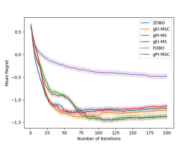
(a) Branin

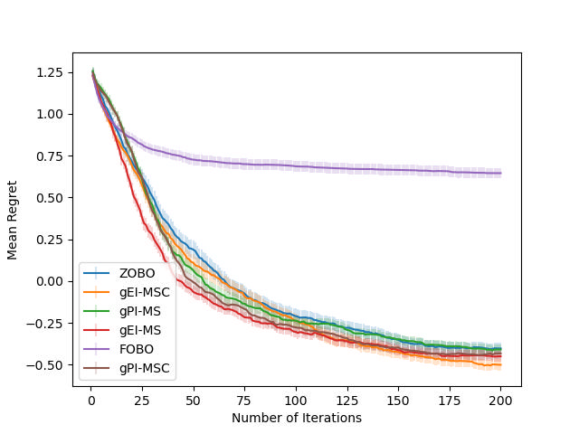
(b) Levy

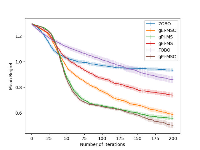
(c) Ackley

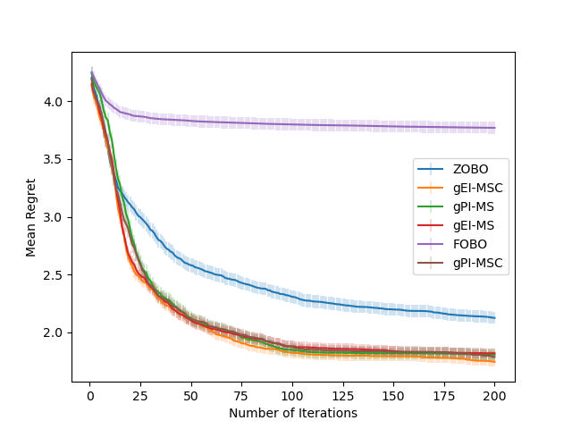
(d) DixonPrice

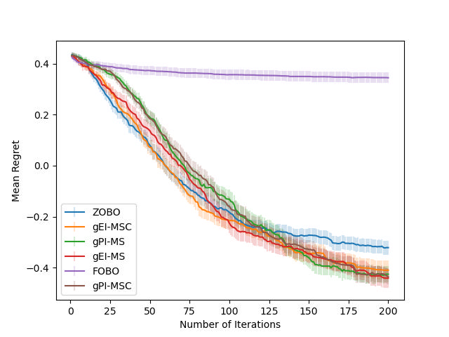
(e) Hartmann

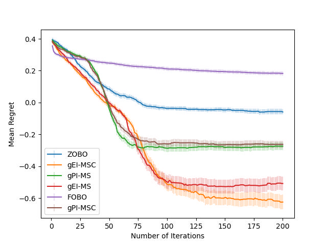
(f) Cosine8

Figure 1: Synthetic Test Functions

4.1 Synthetic test functions

The 6 synthetic test functions considered for performance evaluation are Branin (dimension of the domain d=2), Levy (d=4), Ackley (d=5), DixonPrice (d=5), Hartmann (d=6) and Cosine8 (d=8) from [39]. We minimize these functions which is equivalent to maximizing the negative of the functions. A Gaussian noise with 0 mean and a variance of 0.25 was added to the function and gradient evaluations to test the robustness of the algorithms. We plot the mean of the logarithm of the immediate regret as a function of number of iterations (function evaluations) to compare the performance of the algorithms. Note that the immediate regret is defined as the absolute value of the difference of the maximum of the solutions obtained by the BO method so far and the global maximum. We start with $5$ initial points to fit the GPs and run the algorithms for $200$ iterations. We average the logarithm of immediate regret over $200$ runs to obtain the mean regret. For the gPI and gEI algorithms, the value of $k$ chosen is 10 and this choice of $k$ is arbitrary. However, $k$ can be treated as a hyper-parameter itself and optimized which is left for future work.

From Figure 1, it is evident that gPI and gEI algorithms achieve significantly lower regrets for Ackley, DixonPrice, Hartmann and Cosine8 than ZOBO and FOBO. This shows that our algorithms are able to utilize gradient information in a much more effective way and at the same time distinguish between maxima, minima and saddle points. For Branin, the performance of ZOBO is better than gEI-MS algorithm. In contrast, gPI-MS and gPI-MSC achieve lower regret than ZOBO. However, notice that the logarithm of immediate regret is around $-1.5$ for all the algorithms i.e., the error between the true optimal value and that found by our algorithm is less than $0.1$. Therefore, all the algorithms have almost converged to the true optimal value. For Levy, the performance of all the algorithms is similar. For most of the functions, gPI class of algorithms perform better or similar to gEI. This is because gPI takes into account the function value into the acquisition function itself and therefore, is able to suggest better points. However, gEI performs much better than gPI for Cosine8. Further research is warranted in order to understand where gEI is more suitable than gPI and vice-versa.

4.2 Hyper-parameter Optimization

We perform two experiments on hyperparameter optimization and show that our algorithms work well for optimizing hyper-parameters for machine learning tasks. We obtain the hyper-gradients (gradients w.r.t. hyper-parameters) using the EvoGrad approach described in [6].

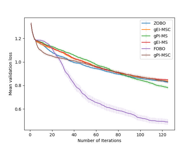
(a) 6D Regularization Problem

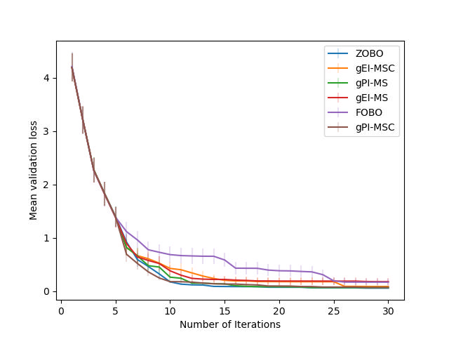
(b) Rotation transformation

Figure 2: Hyper-parameter Tasks

4.2.1 Rotation Transformation

In this experiment we consider MNIST images ([23]).
MNIST images consists of hand-written images of digits from 0-9 and the task is to train an image classifier which can classify images into appropriate digits. We modify the task slightly by rotating the validation and test images by 30°(this information is kept hidden) while the training images are not rotated. If we train a classifier on the un-rotated images, then it will perform poorly on the validation and test data set. Therefore, it becomes imperative to learn the hidden angle by which the validation and test images are rotated. We learn this hidden angle by minimizing the validation loss using BO. For the image classification task, we use LeNet [22] as our base architecture and train it for 5 epochs. We compare the average validation loss over 50 runs. We run each of the BO algorithm for 30 iterations i.e. we train our CNN 30 times with different hyper-parameters. gPI performs better than other algorithms (see Figure 2b). Also, note that all algorithms have converged to $0$ loss.

4.2.2 6D Regularization Problem

In this problem, we minimize a validation loss function $f_{v}(x)=\sum_{i=1}^{6}(x_{i}-i+0.5)^{2}$, where $x\in\mathbb{R}^{6}$. The training loss function used is $f_{T}(x)=\sum_{i=1}^{6}(x_{i}-10i)^{2}+||\lambda^{T}x||^{2}_{2}$, where $\lambda\in[0,100]^{6}$ is a regularization coefficient which we learn by minimizing the validation loss using Bayesian optimization. The validation loss achieves the minimum value of $0$ at $\lambda=[19.00,12.33,11.00,10.43,10.11,9.91]$. We compare the values of the validation loss function achieved by different BO algorithms. We run each BO algorithm for 200 iterations i.e. we query the objective function 200 times (excluding the $5$ initial queries for fitting the GP). We plot the average true validation loss over $200$ runs as a function of number of iterations. We observe from Figure 2a that gPI-MSC outperforms most of the algorithms except for the FOBO algorithm. Initially, FOBO’s performance is poor, however, surprisingly it eventually outperforms other algorithms. Further research is warranted to understand why FOBO performs better than its counterparts in this setting.

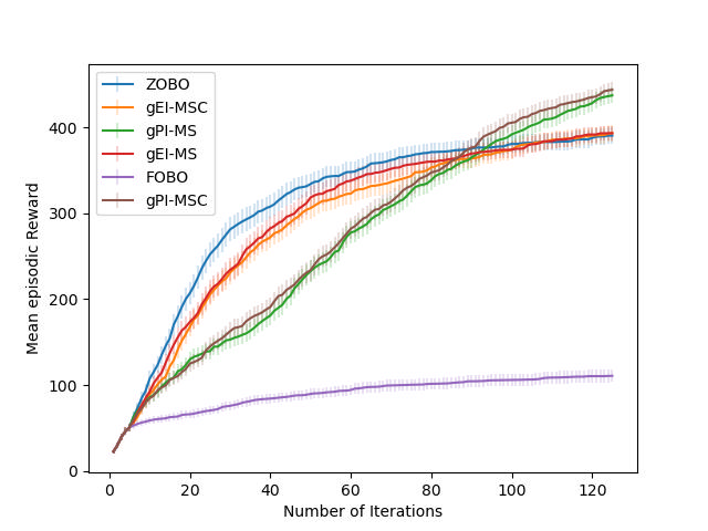
(a) CartPole$-$v1

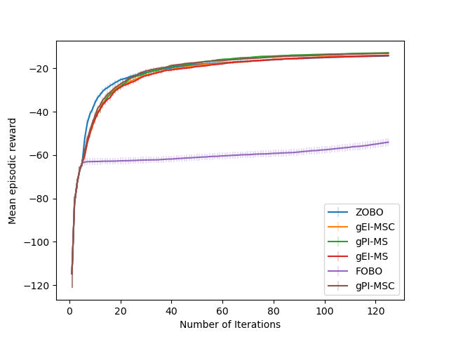
(b) GridWorld

Figure 3: RL Tasks

4.3 RL tasks

Readily available gradient information make RL an interesting domain to apply our gEI and gPI algorithms. We have primarily focused our attention towards integrating policy based methods with BO. Here, the y-axis correspond to mean episodic rewards. The estimates of gradient for policy based methods can be calculated (see supplementary material). We consider Cartpole from the OpenAI gym and a custom grid world task to compare the performance of different BO algorithms. [8].

4.3.1 Cartpole

This task involves balancing a pole by suitably choosing between two actions (left and right) till the episode terminates. We have used a neural network to parameterize the policy. The architecture considered was a simple one layer neural network with 5 hidden units and with no bias. See Figure 3a for performance comparison of all the algorithms. While gPI-MSC and gPI-MS lag behind initially, towards the end they are able to outperform all the algorithms. The performance at the beginning can be attributed to the poor GP fitting and the choice of $\epsilon$ in our gPI acquisition function.

4.3.2 Grid World

The objective of the agent is to find the most optimal path to exit the grid world using four actions (left, right, up, down). The reward in a given state is sampled from an array of rewards [-5,-1,-2,1,2,5,10]. The sampling distribution is Dirichlet distribution and is fixed for each state. Thus, different states have different single-stage rewards. As a result, the shortest path (geometrically) in this grid world need not correspond to the optimal solution. For this problem, we use a one layer neural network with 5 hidden units and with no bias for parameterizing the policy. From Figure 3b, we can see that our algorithms perform at par with ZOBO and outperform FOBO. The performance of our BO algorithms is not that significant over ZOBO and we suspect the choice of our kernel (RBF) do not suit here. Usually RL objective functions are not smooth and kernels as in [1] might prove to be more beneficial.

5 Conclusions & Future work

In this work, we have proposed EI and PI based FOBO algorithms that have a superior performance compared to the state-of-the-art ZOBO and FOBO algorithms. The novelty in our algorithm lies in the design of the acquisition functions that can extract better information from the posterior GP models as compared to the existing FOBO algorithms.

An important line of research would be to perform the regret analysis of the proposed algorithms on the lines of [38], [35]. Another interesting line of research would be to devise FOBO algorithms for time varying BO problems as in [5] and utilize FOBO algorithms in robust-optimization as in [3]. As our results suggests, no single acquisition function (based on EI or PI) can perform very well on all the black-box functions and in-fact we have a portfolio of acquisition functions, each of which can work well for suitable function choices. In such cases, it would be interesting to perform a portfolio allocation procedure to suitably select the appropriate acquisition function each time as in [17].

References

- [1] Aaron Wilson, A.F., Tadepalli, P.: Using trajectory data to improve bayesian optimization for reinforcement learning. Journal of Machine Learning Research (2014)
- [2] Balandat, M., Karrer, B., Jiang, D., Daulton, S., Letham, B., Wilson, A.G., Bakshy, E.: Botorch: a framework for efficient monte-carlo bayesian optimization. Advances in neural information processing systems 33, 21524–21538 (2020)
- [3] Beland, J.J., Nair, P.B.: Bayesian optimization under uncertainty. In: NIPS BayesOpt 2017 workshop (2017)
- [4] Bergstra, J., Yamins, D., Cox, D.: Making a science of model search: Hyperparameter optimization in hundreds of dimensions for vision architectures. In: International conference on machine learning. pp. 115–123. PMLR (2013)
- [5] Bogunovic, I., Scarlett, J., Cevher, V.: Time-varying gaussian process bandit optimization. In: Artificial Intelligence and Statistics. pp. 314–323. PMLR (2016)
- [6] Bohdal, O., Yang, Y., Hospedales, T.: Evograd: Efficient gradient-based meta-learning and hyperparameter optimization. Advances in Neural Information Processing Systems 34, 22234–22246 (2021)
- [7] Brochu, E., Cora, V.M., De Freitas, N.: A tutorial on bayesian optimization of expensive cost functions, with application to active user modeling and hierarchical reinforcement learning. arXiv preprint arXiv:1012.2599 (2010)
- [8] Brockman, G., Cheung, V., Pettersson, L., Schneider, J., Schulman, J., Tang, J., Zaremba, W.: Openai gym. arXiv preprint arXiv:1606.01540 (2016)
- [9] Deshwal, A., Belakaria, S., Doppa, J.R., Kim, D.H.: Bayesian optimization over permutation spaces. In: Proceedings of the AAAI Conference on Artificial Intelligence. vol. 36, pp. 6515–6523 (2022)
- [10] Falkner, S., Klein, A., Hutter, F.: Bohb: Robust and efficient hyperparameter optimization at scale. In: International Conference on Machine Learning. pp. 1437–1446. PMLR (2018)
- [11] Franceschi, L., Donini, M., Frasconi, P., Pontil, M.: Forward and reverse gradient-based hyperparameter optimization. In: International Conference on Machine Learning. pp. 1165–1173. PMLR (2017)
- [12] Frazier, P.I.: A tutorial on bayesian optimization. arXiv preprint arXiv:1807.02811 (2018)
- [13] Golovin, D., Solnik, B., Moitra, S., Kochanski, G., Karro, J., Sculley, D.: Google vizier: A service for black-box optimization. In: Proceedings of the 23rd ACM SIGKDD international conference on knowledge discovery and data mining. pp. 1487–1495 (2017)
- [14] Han, E., Arora, I., Scarlett, J.: High-dimensional bayesian optimization via tree-structured additive models. In: Proceedings of the AAAI Conference on Artificial Intelligence. vol. 35, pp. 7630–7638 (2021)
- [15] Hernández-Lobato, J.M., Hoffman, M.W., Ghahramani, Z.: Predictive entropy search for efficient global optimization of black-box functions. Advances in neural information processing systems 27 (2014)
- [16] Hoang, T.N., Hoang, Q.M., Ouyang, R., Low, K.H.: Decentralized high-dimensional bayesian optimization with factor graphs. In: Proceedings of the AAAI Conference on Artificial Intelligence. vol. 32 (2018)
- [17] Hoffman, M., Brochu, E., De Freitas, N., et al.: Portfolio allocation for bayesian optimization. In: UAI. pp. 327–336. Citeseer (2011)
- [18] Huang, D., Allen, T.T., Notz, W.I., Zeng, N.: Global optimization of stochastic black-box systems via sequential kriging meta-models. Journal of global optimization 34(3), 441–466 (2006)
- [19] Jain, K., K. J., P., Bodas, T.: Bayesian optimization for function compositions with applications to dynamic pricing. arXiv preprint arXiv:2303.11954 (2023)
- [20] Jones, D.R., Schonlau, M., Welch, W.J.: Efficient global optimization of expensive black-box functions. Journal of Global optimization 13(4), 455–492 (1998)
- [21] Kushner, H.J.: A new method of locating the maximum point of an arbitrary multipeak curve in the presence of noise (1964)
- [22] Le Cun, Y., Jackel, L.D., Boser, B., Denker, J.S., Graf, H.P., Guyon, I., Henderson, D., Howard, R.E., Hubbard, W.: Handwritten digit recognition: Applications of neural network chips and automatic learning. IEEE Communications Magazine 27(11), 41–46 (1989)
- [23] LeCun, Y., Cortes, C.: MNIST handwritten digit database (2010), http://yann.lecun.com/exdb/mnist/
- [24] Maclaurin, D., Duvenaud, D., Adams, R.: Gradient-based hyperparameter optimization through reversible learning. In: International conference on machine learning. pp. 2113–2122. PMLR (2015)
- [25] Mockus, J., Tiesis, V., Zilinskas, A.: Toward global optimization, volume 2, chapter bayesian methods for seeking the extremum (1978)
- [26] Müller, S., von Rohr, A., Trimpe, S.: Local policy search with bayesian optimization. Advances in Neural Information Processing Systems 34, 20708–20720 (2021)
- [27] Mutny, M., Krause, A.: Efficient high dimensional bayesian optimization with additivity and quadrature fourier features. Advances in Neural Information Processing Systems 31 (2018)
- [28] Nguyen, D., Gupta, S., Rana, S., Shilton, A., Venkatesh, S.: Bayesian optimization for categorical and category-specific continuous inputs. In: Proceedings of the AAAI Conference on Artificial Intelligence. vol. 34, pp. 5256–5263 (2020)
- [29] Picheny, V., Ginsbourger, D., Richet, Y., Caplin, G.: Quantile-based optimization of noisy computer experiments with tunable precision. Technometrics 55(1), 2–13 (2013)
- [30] Prabuchandran, K., Penubothula, S., Kamanchi, C., Bhatnagar, S.: Novel first order bayesian optimization with an application to reinforcement learning. Applied Intelligence 51(3), 1565–1579 (2021)
- [31] Pyzer-Knapp, E.O.: Bayesian optimization for accelerated drug discovery. IBM Journal of Research and Development 62(6), 2–1 (2018)
- [32] Schulman, J., Wolski, F., Dhariwal, P., Radford, A., Klimov, O.: Proximal policy optimization algorithms. arXiv preprint arXiv:1707.06347 (2017)
- [33] Scott, W., Frazier, P., Powell, W.: The correlated knowledge gradient for simulation optimization of continuous parameters using gaussian process regression. SIAM Journal on Optimization 21(3), 996–1026 (2011)
- [34] Shahriari, B., Swersky, K., Wang, Z., Adams, R.P., De Freitas, N.: Taking the human out of the loop: A review of bayesian optimization. Proceedings of the IEEE 104(1), 148–175 (2015)
- [35] Shekhar, S., Javidi, T.: Significance of gradient information in bayesian optimization. In: International Conference on Artificial Intelligence and Statistics. pp. 2836–2844. PMLR (2021)
- [36] Snoek, J., Larochelle, H., Adams, R.P.: Practical bayesian optimization of machine learning algorithms. Advances in neural information processing systems 25 (2012)
- [37] Srinivas, N.: Gaussian process optimization in the bandit setting: No regret and experimental design. In: Proceedings of the International Conference on Machine Learning, 2010 (2010)
- [38] Srinivas, N., Krause, A., Kakade, S.M., Seeger, M.: Gaussian process optimization in the bandit setting: No regret and experimental design. arXiv preprint arXiv:0912.3995 (2009)
- [39] Surjanovic, S., Bingham, D.: Virtual library of simulation experiments: Test functions and datasets. Retrieved August 15, 2022, from http://www.sfu.ca/~ssurjano (2022)
- [40] Sutton, R.S., McAllester, D.A., Singh, S.P., Mansour, Y.: Policy gradient methods for reinforcement learning with function approximation. In: Advances in neural information processing systems. pp. 1057–1063 (2000)
- [41] Vien, N.A., Zimmermann, H., Toussaint, M.: Bayesian functional optimization. In: Proceedings of the AAAI Conference on Artificial Intelligence. vol. 32 (2018)
- [42] Wang, Z., Zoghi, M., Hutter, F., Matheson, D., De Freitas, N., et al.: Bayesian optimization in high dimensions via random embeddings. In: IJCAI. pp. 1778–1784. Citeseer (2013)
- [43] White, C., Neiswanger, W., Savani, Y.: Bananas: Bayesian optimization with neural architectures for neural architecture search. In: Proceedings of the AAAI Conference on Artificial Intelligence. vol. 35, pp. 10293–10301 (2021)
- [44] Williams, C.K., Rasmussen, C.E.: Gaussian processes for machine learning, vol. 2. MIT press Cambridge, MA (2006)
- [45] Wu, J., Poloczek, M., Wilson, A.G., Frazier, P.: Bayesian optimization with gradients. Advances in neural information processing systems 30 (2017)