Multilevel Surrogate-based Control Variates
Abstract
Monte Carlo (MC) sampling is a popular method for estimating the statistics (e.g. expectation and variance) of a random variable. Its slow convergence has led to the emergence of advanced techniques to reduce the variance of the MC estimator for the outputs of computationally expensive solvers.
The control variates (CV) method corrects the MC estimator with a term derived from auxiliary random variables that are highly correlated with the original random variable. These auxiliary variables may come from surrogate models. Such a surrogate-based CV strategy is extended here to the multilevel Monte Carlo (MLMC) framework, which relies on a sequence of levels corresponding to numerical simulators with increasing accuracy and computational cost. MLMC combines output samples obtained across levels, into a telescopic sum of differences between MC estimators for successive fidelities.
In this paper, we introduce three multilevel variance reduction strategies that rely on surrogate-based CV and MLMC. MLCV is presented as an extension of CV where the correction terms devised from surrogate models for simulators of different levels add up. MLMC-CV improves the MLMC estimator by using a CV based on a surrogate of the correction term at each level. Further variance reduction is achieved by using the surrogate-based CVs of all the levels in the MLMC-MLCV strategy. Alternative solutions that reduce the subset of surrogates used for the multilevel estimation are also introduced.
The proposed methods are tested on a test case from the literature consisting of a spectral discretization of an uncertain 1D heat equation, where the statistic of interest is the expected value of the integrated temperature along the domain at a given time.
The results are assessed in terms of the accuracy and computational cost of the multilevel estimators, depending on whether the construction of the surrogates, and the associated computational cost, precede the evaluation of the estimator. It was shown that when the lower fidelity outputs are strongly correlated with the high-fidelity outputs, a significant variance reduction is obtained when using surrogate models for the coarser levels only. It was also shown that taking advantage of pre-existing surrogate models proves to be an even more efficient strategy.
Keywords: Multifidelity, multilevel Monte Carlo, control variates, surrogate models, polynomial chaos, variance reduction.
1 Introduction
In recent years, the propagation of uncertainties in numerical simulators has become an essential step in the study of physical phenomena. Therefore, uncertainty quantification (UQ) has emerged as an important element in scientific computing [50, 52]. For complex nonlinear systems, the task of quantifying the effect of uncertainties on the simulator behaviour can pose major challenges as closed-form solutions often do not exist. Sampling-based algorithms are considered the default approach when it comes to UQ for complex nonlinear simulators. The Monte Carlo (MC) sampling method is the most popular and flexible method in UQ. Here, statistical information is extracted from a -sample of simulator responses. Due to its non-intrusive nature, MC is straightforward to implement. On the one hand, the convergence of an MC statistic is independent of the dimension, but on the other hand, it is very slow, namely at a rate of . For computationally expensive simulators, the cost of MC is often considered impractically high. In some cases, slight improvements can be obtained through the use of importance sampling [27], latin hypercube sampling [35] or quasi-Monte Carlo (QMC) [13].
Another well-known approach in UQ consists in replacing the simulator by a surrogate model. Fast-to-evaluate surrogates can be used to approximate the high-fidelity model response and therefore reduce drastically the computational cost of estimating statistics. Polynomial chaos (PC) [34, 37], Gaussian process models [45], radial basis functions [41] and (deep) neural networks [54] are commonly used surrogate models. The downside of the surrogate-based approach is that it introduces approximation error, which causes biases in the statistics estimators. Besides, this approximation error tends to increase in high dimension.
One recent MC sampling framework based on control variates (CV) [29, 31, 30, 33] has been extensively developed and used. In a sampling-based CV strategy, one seeks to reduce the variance of the MC estimator of a random variable, arising from the high-fidelity model, by exploiting its correlation with an auxiliary random variable that arises from low-fidelity models approximating the same input-output relationship. In classic CV theory, the mean of the auxiliary random variable is assumed to be known. Unfortunately, in many cases such an assumption is not valid. This creates the need to use another estimator for the auxiliary random variable [24, 44, 43, 42, 39], which involves an additional computational cost. Recently, the adoption of surrogate models as such auxiliary random variables, in particular PC models, has been explored in [16, 56, 17, 25]. The benefits are twofold: (1) the prediction of the surrogate models may be highly correlated with the output high-fidelity model, leading to a reduced variance of the CV estimator as compared to the MC estimation; (2) certain surrogate models provide exact statistics that are needed by the CV approach. Another variance reduction technique, called the multilevel MC (MLMC) method [21, 10, 22], uses a hierarchy of models. Originally devised for the estimation of expected values, MLMC has since been extended to the estimation of other statistics, see, e.g., [4, 5] for the estimation of variance and higher order central moments and [36] for the computation of Sobol’ indices. Typically, multilevel methods are based on a sequence of levels which correspond to a hierarchy of simulators with increasing accuracy and cost. From a practical standpoint, the different levels often correspond to simulators with increasing mesh resolutions. This translates into a lower accuracy of the so-called coarse levels, whereas the finer levels correspond to accurate simulators. By construction, MLMC results in an unbiased estimator. It relies on a telescopic sum of terms based on the differences between the successive simulators. It debiases the MC estimator associated with the lowest-level simulator. Many other unbiased multilevel estimators have been devised in recent years. The multi-index MC estimator [26] is an extension of the MLMC estimator such that the telescoping sum idea is used in multiple directions. In [23], the authors developed a variant of MLMC which uses QMC samples instead of independent MC samples for each level. Multi-fidelity MC (MFMC) estimators [19, 18] are another extension that is based on the CV approach. Recently, the authors in [48, 47] took a different approach by formulating a multilevel estimator as the result of a linear regression problem.
In this work, we combine multilevel sampling with surrogate-based CV to define new estimators with the advantages of both. These novel multifidelity variance reduction strategies allow us to quantify efficiently the output uncertainties of simulators with limited computational budgets. A first strategy, named multilevel control variates (MLCV), uses CVs based on surrogate models of simulators corresponding to different levels. Although this strategy does not build on the MLMC approach specifically, it still exploits multilevel information through the surrogates constructed at different levels. The second strategy, named multilevel Monte Carlo with control variates (MLMC-MLCV), utilizes CV in an information fusion framework to exploit synergies between the flexible MLMC sampling and the correlation shared between the high- and low-fidelity components. The numerical results show that the unbiased MLMC-MLCV estimators can converge faster than the existing estimators.
The paper is organized as follows. We introduce notations and the necessary mathematical background in section 2. In section 3, we briefly discuss the MLMC estimator and then define our proposed MLMC-MLCV estimator that combines multilevel sampling and surrogate-based CV. In section 4, we conduct numerical experiments to support the theoretical results. Section 5 proposes concluding remarks.
2 Background
In this section, we summarize the important results of statistical estimation using control variates and we show how surrogate models can be leveraged in this setting.
2.1 Notation
We first introduce a few notations. Throughout the rest of this paper, the high-fidelity numerical model is abstractly represented by the deterministic mapping
| (1) |
where is a vector of uncertain input parameters evolving in a measurable space denoted by , with . Following a probabilistic approach, the inputs are assumed to be continuous random variables , defined on a probability space , with known probability density functions (PDFs) . They are assumed to be independent, so that the PDF of the random vector is . In this work, we seek an accurate estimator of some statistic of the output random variable , e.g., its expected value () or variance (), at a reasonable computational cost .
2.2 Crude Monte Carlo
In practice, the MC estimator of the statistic is based on observations defined as where is a -sample of , that is, a collection of independent and identically distributed random variables with the same distribution as . For instance, the sample mean and (unbiased) sample variance estimators,
| (2) |
are MC estimators of the expectation and variance of , respectively. It is well known that these estimators are unbiased, that is, , so that the mean square error (MSE) of reduces to the variance of the estimator:
| (3) |
The convergence of these MC estimators is known to be slow, so that variance reduction techniques are needed when dealing with computationally expensive simulators.
2.3 Control variates
In this section, we present a well-known variance reduction technique using auxiliary random variables as control variates. We denote by the statistics of the control variates that correspond to the statistic that we seek to estimate. These control statistics are assumed to be known exactly. Then, the CV estimator is defined as
| (4) |
where and are unbiased MC estimators of and , respectively, based on a common input -sample , and where is the control parameter. We note that the CV estimator is unbiased by construction, regardless of the value of the parameter , and that its variance reads
| (5) |
with and . To fully take advantage of the control variates, the parameter is selected so as to minimize the variance (5) of the CV estimator. Assuming that the covariance matrix is non-singular (and thus symmetric positive definite, SPD), the first- and second-order optimality conditions of the minimization problem imply that there exists a unique optimal solution,
| (6) |
The optimal CV estimator is thus , and its variance is given by
| (7) |
where is nonnegative, as is SPD. Denoting by the diagonal matrix consisting of the diagonal of , it can be shown further that , where is the vector of the Pearson correlation coefficients between and , and is the correlation matrix of . Thus, corresponds to the squared coefficient of multiple correlation between and the elements of [1, section 2.5.2]. Consequently, , and we refer to as the variance reduction factor of the CV estimator. This shows that the variance of the optimal CV estimator is always reduced (or, rigorously speaking, not increased) compared to the MC estimator . Furthermore, the higher , the greater the reduction in variance.
Remark 1.
The requirement that be non-singular is a reasonable one. Indeed, let us suppose that is singular. Then, because is positive semi-definite by construction, this implies that there exists a nonzero vector such that , indicating that any one element of can be expressed as an affine function of the others. As such, it does not bring any additional information to the CV estimator, so that at least one of the control variates can simply be discarded.
A desirable property of the CV estimator is that increasing the number of control variates improves the CV estimator. Specifically, under mild assumptions, proposition 1 states that the variance of the CV estimator is reduced (or, rigorously speaking, not increased) when adding a new control variate.
Proposition 1.
Let , , and define , and . We further assume that and are non-singular and that . Let , with , be the optimal CV estimator based on control variates, and let denote its variance reduction factor. Then .
Proof.
We have , where and , and where and . Note that and are both non-singular, because so are and . The augmented matrix may be inverted by block using the Schur complement of the (1,1)-block . It follows that . Now, because is SPD (it is positive semidefinite by construction and non-singular by assumption), for any choice of . The particular choice of implies that , which in turn implies that . ∎
Corollary 1.
Under the assumptions of proposition 1, the equality holds if and only if .
Proof.
Straightforward from with . ∎
For the CV estimation of specific statistics, the expressions of and may be further reduced to involve statistics on and directly. These expressions, as well as the consequences on eqs. 6 and 7, are given in appendix A for the CV estimators of and .
It should be noted at this point that, in practice, the optimal parameter needs to be approximated. Specifically, the statistics involved in and need to be estimated. This can be done either using the same sample as for the CV estimator itself, or using an independent, pilot sample . The former strategy introduces a bias in the resulting CV estimator, while the latter guarantees unbiasedness but requires additional high-fidelity simulator evaluations, so that the former strategy is generally preferred. Besides, statistical remedies such as jackknifing, splitting or bootstrapping have been proposed to reduce or eliminate the bias introduced by the former strategy [38]. In both strategies, however, neither the theoretical variance reduction given by eq. 7 nor proposition 1 hold anymore.
Remark 2.
In some instances, because it only involves the control variates, may be known exactly (see remark 3 for an example in a multilevel setting involving PC-based control variates) or estimated accurately using many independent samples at negligible cost. Unfortunately, this is not the case for , which involves the output of the high-fidelity simulator .
2.4 Surrogate-based control variates
The efficiency of the CV approach relies on the strong correlation between and the control variates . In a multifidelity framework, the control variates correspond to the output of low-fidelity versions of , typically in the form of simulators with simplified physics and/or coarser discretization. In many applications, the exact statistical measures of such control variates may not be available. One way to circumvent this limitation is to use additional samples to also estimate . This type of estimators led to an approximate CV class of methods [24, 39, 43], where different model management and sample allocation strategies may be used to find a suitable trade-off between the additional cost of sampling and the resulting variance reduction. Recently, an optimal strategy was proposed [48, 49, 47] leading to the so-called multilevel best linear unbiased estimator (MLBLUE), as well as a unifying framework for a large class of multilevel and multifidelity estimators.
In this paper, we focus on the case where the low-fidelity models correspond to surrogate models of the high-fidelity simulator . The main advantage is that the statistics may, in some instances, be directly available, or at least may be estimated arbitrarily accurately at negligible cost, so that the original CV approach described in section 2.3 can be used. Using surrogate models in a CV strategy has been explored previously in [16, 56], where the available computational budget is allocated both to the construction of the surrogates and to the actual CV estimations. In [56], the authors introduce an approach that optimally balances the computational effort needed to select the optimal degree of the polynomial chaos (PC) expansion used in a stochastic Galerkin CV approach. In our work, we focus on the situation in which the surrogate models are available, so that we do not consider any optimization strategy for the construction of the surrogates. Nevertheless, for the fairness of comparison, we still report the pre-processing cost of contructing the surrogate models.
We now briefly describe three different surrogate models commonly used in a UQ framework, and discuss the availability of statistics of their output.
2.4.1 Gaussian process modelling
We assume that the simulator is a realization of a Gaussian process (GP) indexed by and defined by its mean function and covariance kernel ,
| (8) | ||||
| (9) |
In practice, one can parametrize the forms of and . For example, in the widely used ordinary GP method, a stationary GP is assumed. In this case, is set as a constant . More importantly, it is assumed that , and is a constant. Popular forms of kernels include polynomial, exponential, Gaussian, and Matérn functions. For example, the Gaussian kernel can be written as , where the weighted norm is defined as where are correlation lengths. The hyperparameters and can be obtained by maximum likelihood. Then, given observations of at , the posterior of can be defined as
| (10) |
whose expectation and covariance are given by
| (11) | ||||
| (12) |
Thereafter, the high-fidelity model at will be approximated by the conditional expectation,
| (13) |
Thus, the expectation and variance of are defined as
| (14) | ||||
| (15) |
These two statistics can be approximated empirically by taking a large sample of , as the GP model is inexpensive. Analytical formulas exist for some pairs of distributions and covariance functions (see [8, Table 1] and [28, 15]).
2.4.2 Taylor polynomials
We assume that the numerical simulator is infinitely differentiable and that the moments of are finite. Under this assumption, it is possible to expand the original simulator around the input’s expected value as the infinite polynomial series according to Taylor’s theorem,
| (16) |
where , , , and . Thus, the function may be approximated by the first- and second-order Taylor polynomials,
| (17) | ||||
| (18) |
where and are the Jacobian and Hessian matrices of at , respectively. In practical computations, the derivatives may be approximated by numerical differentiation if they are not provided. The expectation and variance of and are then defined as
| (19) | ||||
| (20) | ||||
| (21) | ||||
| (22) |
where for any matrix , denotes the element-wise square of , is the trace of , is the element-wise variance of , and .
2.4.3 Polynomial chaos expansion
We consider the truncated polynomial chaos (PC) expansion of [55, 9, 20, 32],
| (23) |
where the coefficients are real scalars and are orthonormal multivariate polynomials:
| (24) |
where denotes the Kronecker delta. The coefficients may be approximated using non-intrusive techniques such as non-intrusive (pseudo)spectral projection [46, 12, 11], regression [3, 51, 6, 7], interpolation [2, 40], or from intrusive approaches such as the stochastic Galerkin method [20, 32]. Assuming , the expectation and variance of are then given by
| (25) |
3 Multilevel estimators
In this section, we present so-called multilevel statistical estimation techniques based on a sequence of simulators , with increasing accuracy and computational cost, where denotes the high-fidelity numerical simulator. The levels are ordered from the coarsest () to the finest (). We denote by the random variable and the statistic of increasingly close to .
3.1 Multilevel Monte Carlo
The statistic can be expressed as the telescoping sum
| (26) |
where , and, by convention, . The MLMC estimator of is then defined as [21, 22, 53]
| (27) |
where, at each level , is an unbiased MC estimator of , based on an input sample such that the members of and are mutually independent for . In many instances, is actually defined as , where denotes the unbiased MC estimator of based on the simulator using the -sample .
For example, the MLMC estimator of the expectation is given by
| (28) |
where , with . We stress that the correction terms at each level are computed from the same input sample , but using two successive simulators, and . Similarly, the MLMC estimator of the variance is defined as [4]
| (29) |
where is the single-level unbiased MC variance estimator. Owing to the independence of the estimators , the variance of the MLMC estimator is
| (30) |
In practice, the MLMC method relies on the allocation of the total (expected) computational cost of the MLMC estimator across the different levels, with
| (31) |
where is the (expected) cost of one evaluation of the simulator , with by convention. Thus, a key aspect is played by the choice of the number of samples allocated to each level . The goal is to find the sample sizes that minimize the variance of the estimator given a computational budget . Thus, the sample allocation problem reads
| (32) | ||||||
| subject to |
This minimization problem has a unique solution which can be computed analytically (see, e.g., [21, 10, 36]). In practice, is not known, and we instead rely on the assumption that , with independent of [53, 36]. This is a reasonable assumption that holds for the MLMC estimation of the expectation, variance and covariance [36, Table 1]. Note that, for the estimation of the expectation, we have , with and . The sample allocation problem eq. 32 is then replaced with
| (33) | ||||||
| subject to |
which is equivalent for the expectation, and an approximation for other statistics.
3.2 Multilevel surrogate-based control variate strategies
In this section, we introduce various surrogate-based control variate strategies in a multilevel framework where a hierarchy of simulators is available. These strategies rely on using the random variables as control variates, where is a surrogate model of the simulator .
3.2.1 Multilevel control variates (MLCV)
The first strategy, referred to as multilevel control variates and hereafter abbreviated MLCV, consists of using the surrogate models at all levels to build the control variates in eq. 4. Thus, corresponds to the statistical measure of the random variable , and to its unbiased MC estimator. For instance, the MLCV estimator of the expectation based on an -sample reads
| (34) |
where , , and . Note that this approach does not build on the MLMC methodology described in section 3.1, but still exploits multilevel information through the surrogates constructed at different levels.
3.2.2 Multilevel Monte Carlo with control variates (MLMC-CV)
The second strategy consists of improving the MLMC estimator eq. 27 using the surrogate-based control variates . Specifically, the MLMC-CV estimator improves the MC estimation of each of the correction terms of the MLMC estimator by using a surrogate model of the corresponding correction term as a control variate. Note that the MLMF approach proposed in [18, 19] is based on a similar strategy, using arbitrary low-fidelity models at level in an approximate CV setting. The MLMC-CV estimator reads
| (35) |
where is the CV estimator of the multilevel correction term (cf. eq. 26),
| (36) |
with an unbiased MC estimator of the control variate statistic , based on the same input sample as , again with members of and being independent for . Note that, in eq. 36, because a single control variate is used at each level, the definition of is used in the specific case where . The more general definition when and are not necessarily equal will be useful later in section 3.2.3, where we consider multiple control variates per level. In practice, may be defined as , where is an unbiased estimator of using the -sample .
The optimal value for is obtained individually for each as the optimal (single) CV parameter for ,
| (37) |
and the resulting variance of the control variate estimator of the correction is
| (38) |
The correction estimators being mutually independent, the variance of the optimal MLMC-CV estimator is
| (39) |
indicating that the variance of the MLMC-CV estimator is smaller (as long as ) than that of the MLMC estimator; see eq. 30. We remark that the variance reduction depends on the (squared) correlation between and , which, in turn, typically relates to some measure of similarity between high-fidelity corrections and the corresponding CV corrections (see appendix A for the expectation and variance estimators in a single-level setting).
In our surrogate-based approach, we may define control variates as , where is a surrogate of , so that and could be estimated using samples of and , respectively. It is then crucial to construct the surrogates such that their successive differences are good approximations of , to ensure a high similarity between and . However, constructing as a surrogate of does not give any guarantee on the quality of as a surrogate of . Instead, in addition to the surrogates models of , we construct surrogate models of the differences , and we define auxiliary surrogate models , for . On each level , we then use samples of and for the estimation of and , respectively. As a result, the variance reduction now depends on the similarity between and , where has been constructed to ensure such a similarity. Specifically, for the expectation, the MLMC-CV estimator reads
| (40) |
with optimal values of given by (see section A.1, with )
| (41) |
resulting in level-dependent reduction factors , where
| (42) |
is the squared correlation coefficient between and . It should be noted that, because of the linearity of the expectation operator and its MC estimator, the use of is superfluous. Indeed, we may directly define the MLMC-CV estimator of the expectation as
| (43) |
with . For the variance, the MLMC-CV estimator reads
| (44) |
with and . The resulting level-dependent reduction factors are then related to the correlation between and (see section A.2, with ). Further details on the construction of will be given in section 4.
3.2.3 Multilevel Monte Carlo with multilevel control variates (MLMC-MLCV)
We now propose to further improve the MLMC-CV estimator eq. 35 by combining MLMC with the MLCV approach described in section 3.2.1, resulting in the MLMC-MLCV method. The approach consists in using, at each level , the surrogate-based control variates of all the levels , rather than only using those of level , as was previously done with the MLMC-CV approach.
The MLMC-MLCV estimator then reads
| (45) |
where denotes the CV parameter at level , and is the MLCV estimator of ,
| (46) |
with
| (47) | ||||||
| (48) |
and with and defined as in section 3.2.2.
Because each term eq. 46 is an unbiased (multiple) CV estimator of , the resulting estimator eq. 45 is also unbiased, and the optimal (variance minimizing) value of is given individually for each as the optimal (multiple) CV parameter for ,
| (49) |
The resulting variance is given by
| (50) |
with
| (51) |
Again, owing to the fact that , the variance of the MLMC-MLCV estimator is always less than or equal to the variance of the MLMC estimator given by (see eq. 30).
In our surrogate-based approach, surrogate-based control variates can be used for the coarsest level , namely , so that . At correction levels , we can use control variates based on and , as described in section 3.2.2, so that , for .
The MLMC-MLCV estimator of the expectation is defined by eq. 45, with
| (52) | ||||
| (53) |
where
| (54) | ||||||
| (55) |
The optimal values of the CV parameters are given by
| (56) | ||||||||
| (57) |
resulting in , for . Note that is the same for all . The optimal MLMC-MLCV variance estimator is derived in appendix B.
Remark 3.
In practice, and may be estimated using either a pilot sample or the same sample as for the estimation of and . Alternatively, in the specific context of PC-based control variates, for the estimation of the expectation, a closed-form expression for can be obtained. Letting and , we have
| (58) | ||||
| (59) |
3.3 Practical details
A summary of the methods is presented in table 1. We remark that all the MLMC-like estimators (including the MLMC estimator), hereafter abbreviated MLMC-*, have variance , with
For all these methods, we will further assume that (see section 3.1), which implies that , with .
| Method | Form of the estimator | Eq. |
|---|---|---|
| Monte Carlo (MC). | ||
| Control Variates (CV) [29, 31, 30, 38, 33]. | . | 4 |
| Multilevel Monte Carlo (MLMC) [21, 22]. | . | 27 |
| Multilevel Control Variates (MLCV). CV method where the CVs are based on surrogate models of simulators of different levels of fidelity. | . | 4 |
| MLMC-CV. MLMC with one CV at each correction level based on surrogate models of the simulators on the corresponding level. Corresponds to a surrogate-based MLMF [18, 19] where the exact statistics of the CVs are known. | . | 35, 36 |
| MLMC-MLCV. MLMC-CV with the CVs based on the surrogate models on level 0 and on on levels . | . | 45, 46 |
| MLMC-CV[0]. MLMC-CV using only one CV based on the surrogate on level 0 and no CVs on levels | . | |
| MLMC-MLCV[0]. MLMC-MLCV using only CVs based on the surrogates and on level 0, and on levels . | . |
In the surrogate-based variants of MLMC, the cost of evaluating the surrogate models is assumed to be negligible compared to the costs of evaluating the simulators . Therefore, the total computational cost of the MLMC-* estimator reduces to the cost of the MLMC estimator, , given by eq. 31. Similarly to the case of the MLMC estimator (see, e.g., [36]), the optimal sample sizes such that is minimal under a constrained computational budget of are given by
| (60) |
so that . As a consequence,
| (61) |
with an equality between the left- and right-hand sides for the expectation estimators.
In practice, is not known and must be estimated for each level. In this work, we consider the sequential algorithm proposed in [36, Algorithm 2] for the MLMC. The algorithm starts from an initial, small number of samples on each level. Then, it selects the optimal level on which to increase the sample size by an inflation factor , i.e. the level on which the reduction in total variance relative to the additional computational effort achieved by inflating the sample size by is maximal.
4 Numerical experiments
We demonstrate the value of our MLMC-MLCV method on the uncertain heat equation problem proposed in [18] and summarized in section 4.1. The surrogate models used for the control variates are described in section 4.2, and the results from numerical experiments are presented and discussed in section 4.3.
4.1 Problem description
We consider the partial differential equation describing the time-evolution of the temperature in a 1D rod of unit length over the time interval , with uncertain (random) initial data and thermal diffusivity ,
| (62) |
where is a random vector modelling the uncertainty in the input parameters, and where almost surely. The solution of eq. 62 may be expressed as
| (63) |
with
| (64) |
The initial condition is chosen to have the same prescribed form as in [18]. Specifically, we consider with
| (65) | ||||
| (66) | ||||
| (67) | ||||
| (68) |
which allows to control the spectral content of the solution . Furthermore, as in [18], the diffusion coefficient is modelled by . The random output variable of interest is defined as the integral of the temperature along the rod at final time ,
| (69) | ||||
| (70) | ||||
| (71) |
where . In this experiment, we seek to estimate the expectation , for a given uncertain setting. Consistently with [18], we consider the random variables to be independent and distributed as
| (72) |
The expected value is then given by
| (73) |
where
| (74) |
Finally, we set , and , resulting in .
Numerically, is approximated by truncating the Fourier expansion in eq. 70 to modes and by approximating the integrals in eqs. 70 and 64 by a trapezoidal quadrature rule with equispaced nodes in . The multilevel hierarchy of simulators is then defined according to the number of quadrature nodes used for the approximation at level . Specifically, is approximated at level by
| (75) |
with
| (76) |
where are the pairs of quadrature nodes and associated weights on level . It is then natural to assume that the computational cost of an evaluation of is . The statistic of interest is thus , whose MC estimator will represent the baseline estimator for our experiments. Besides, the quality of all the presented estimators will be assessed in terms of their root mean square error (RMSE) w.r.t. the exact statistic given by eq. 73.
In the following experiments, we set the number of quadrature nodes and the number of levels to 4 (i.e. ). Furthermore, we set so that evaluating is twice as expensive as evaluating . Table 2 summarizes the number of quadrature nodes and the evaluation cost per level. Note that the costs are normalized so that .
| 0 | 1 | 2 | 3 | |
|---|---|---|---|---|
| 15 | 30 | 60 | 120 | |
| 0.125 | 0.25 | 0.5 | 1 | |
| 0.125 | 0.375 | 0.75 | 1.5 |
4.2 Surrogate models
We will mostly use PC models (see section 2.4.3) for the surrogate-based CV estimators. Constructing high-quality surrogates in 7 dimensions can be hard, especially in the presence of non-linearities and with a limited sample size. To avoid overfitting, we resort to the least angle regression (LARS) procedure [14], which is a model-selection regression method that promotes sparsity. More precisely, we employ the basis-adaptive hybrid LARS algorithm proposed by [7, Fig. 5] for the selection of sparse PC bases. For a given design of experiment (DoE) for the PC surrogate construction, this algorithm applies the LARS procedure on candidate PC bases of increasing total polynomial degree , resulting for each in the selection of a limited number of basis polynomial functions. For each , a PC surrogate is constructed by classical least-squares regression on the corresponding reduced (or active) PC basis , and its quality is estimated using a corrected leave-one-out cross-validation procedure [7]. The best surrogate according to this quality measure is eventually retained, and the associated reduced PC basis is denoted by .
In our experiments, we set and the construction budget to 400 times the evaluation cost of , i.e. . This budget is distributed equally among the different levels, so that the associated evaluation cost on each level corresponds to the cost of 100 evaluations, i.e. , as reported in tables 3 and 4. Once constructed, the quality of a surrogate of is assessed in terms of the measure,
| (77) |
estimated using a test sample of size , which is more robust than the corrected leave-one-out measure used for the model selection. The higher the value, the higher-quality the associated surrogate.
For the MLCV estimator, we learn a PC model of from a training DoE of size generated by latin hypercube sampling (LHS) improved by simulated annealing. The training DoE samples for the surrogate construction are different for each level and independent. Table 3 summarizes the properties of the different PC models. Except for , which is built with only 100 points, all the PC models have a good , greater than 0.8. We observe that the basis-adaptive LARS algorithm has selected a decreasing polynomial degree with level , while retaining only a limited number of polynomials in these reduced bases. Thus, although and have distinct degrees, the sizes of the associated reduced bases are similar.
| PC models | ||||
|---|---|---|---|---|
| 800 | 400 | 200 | 100 | |
| 10 | 8 | 6 | 4 | |
| 211 | 77 | 74 | 14 | |
| 0.98 | 0.94 | 0.86 | 0.59 |
For the MLMC-based estimators, we learn a PC model of for and a PC model of for . In practice, training points used for the construction of may be reused for the construction of using nested DoEs. However, it should be noted that the generation of nested LHS DoEs is not as straightforward as for purely random DoEs. While using nested random DoEs is a perfectly valid strategy, we opt for an alternative choice based on LHS. Specifically, we first generate a DoE of size using LHS improved by simulated annealing. Then, for , we sequentially extract a DoE of size . The subset is selected such that it has minimal centered discrepancy among a pool of 1 million random candidate subsets. Table 4 summarizes the properties of these different PC models. The PC models again have a quality measure higher than 0.8, except for and , which were constructed from only 100 evaluations. Note that the values of , and are of the same order of magnitude as those of the PC surrogate models reported in table 3.
| PC models | |||||||
|---|---|---|---|---|---|---|---|
| 800 | 400 | 200 | 100 | 400 | 200 | 100 | |
| 10 | 8 | 8 | 2 | 9 | 7 | 5 | |
| 211 | 83 | 57 | 6 | 112 | 71 | 30 | |
| 0.98 | 0.95 | 0.86 | 0.21 | 0.99 | 0.82 | 0.63 |
4.3 Results
First, in section 4.3.1, we illustrate the use of one or several control variates to reduce the variance of a single-level MC estimator. Then, we compare the MLCV and MLMC-MLCV approaches with the MC and MLMC estimators in section 4.3.2, and we discuss variants of the MLMC-CV and MLMC-MLCV approaches, considering only a limited subset of the surrogate models, in section 4.3.3. We conclude the analysis by reporting the estimation budget allocation across levels resulting from the various MLMC-based methods in section 4.3.4. In practice, all the MLMC-based estimators are built using algorithm 1. Unless stated otherwise, the parameters are set to and for . The quality of the various estimators will be assessed in terms of their RMSE w.r.t. , estimated from 500 repetitions of the experiment.
4.3.1 Single-level MC and control variates
In this first part, we consider only the finest simulator and try to reduce the variance of the MC estimator of by means of surrogate-based CVs. For that purpose, we consider a first-order Taylor polynomial expansion around (see sections 2.4.2 and C) and the PC model described in table 3.
| 1.00 | 0.80 | 0.57 | |
| 0.80 | 1.00 | 0.64 | |
| 0.57 | 0.64 | 1.00 |
Table 5 shows that is well correlated with , with a Pearson coefficient of 0.8, while is less so, with a coefficient of 0.57, which may be explained by the strong non-linearity of . According to eq. 7, these correlation coefficients lead to a theoretical variance reduction factor of 64% when using as a single CV, and of about 32% when using as a single CV. Using both CVs results in a reduction factor of 65%. This minor increase in can be explained by the modest correlation coefficient of 0.64 between and . Note that a reduction factor of in the variance corresponds to a reduction factor of in the standard deviation.
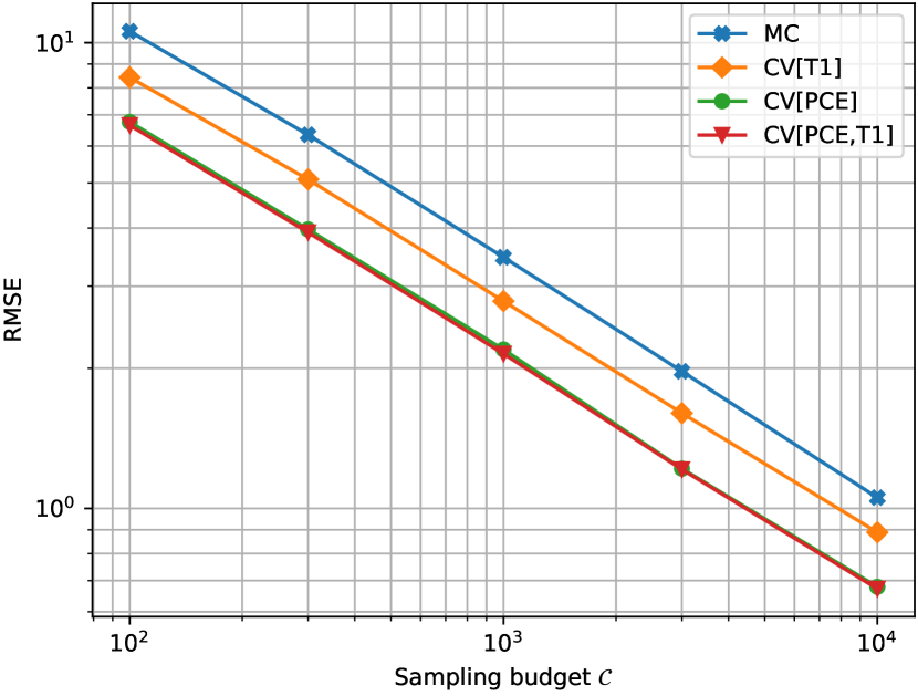
These theoretical expectations are reflected in fig. 1(a) with an RMSE reduction of about 20% when using and 40% when using alone or jointly with . This figure confirms that provides a better CV than , reducing the RMSE of the MC estimator twice as much, regardless of the computational budget. However, the construction cost of the surrogate is not the same. While constructing requires only one evaluation of and its Jacobian matrix, namely at , the construction of involved 100 evaluations. In the case where the surrogate is built specifically for the estimation of the statistic, the real estimation cost is higher as it includes this construction cost. Figure 1(b) illustrates this difference by including the surrogate construction cost in the total evaluation cost. As a result, a significant offset appears when using , since part of the computational budget (namely 100) is used for the surrogate construction and thus not for the estimation. Specifically, the RMSEs of the CV estimators using get below that of the CV estimator using only for a budget of 300 evaluations. For budgets under 200, using only is preferable, even without the analytical gradient available, which would then incur a construction cost of 8 evaluations to approximate the gradient using finite differences. This figure also illustrates proposition 1, that is, increasing the number of control variates improves (rigorously speaking, does not deteriorate) the variance of the CV estimator.
4.3.2 MLCV and MLMC-MLCV
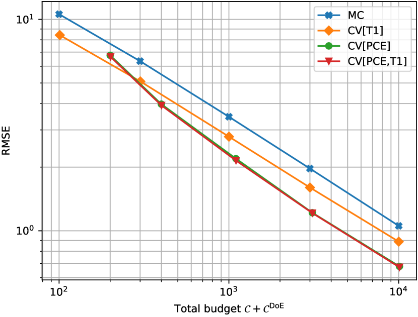
Figure 2 compares the MLCV and MLMC-MLCV estimators proposed in eqs. 34 and 45 with the classical MC and MLMC estimators. This comparison is repeated for different budgets , expressed in terms of the equivalent number of evaluations. Note that the MC and MLCV estimators only use evaluations of the finest simulator , so that , while MLMC-based estimators use all the simulators, so that is given in terms of the MLMC cost eq. 31, indeed corresponding to the equivalent number of evaluations, since the costs are normalized such that . From here on, only PC-based surrogates will be used, so that we omit the superscript “PC” in the notations of the surrogate models.
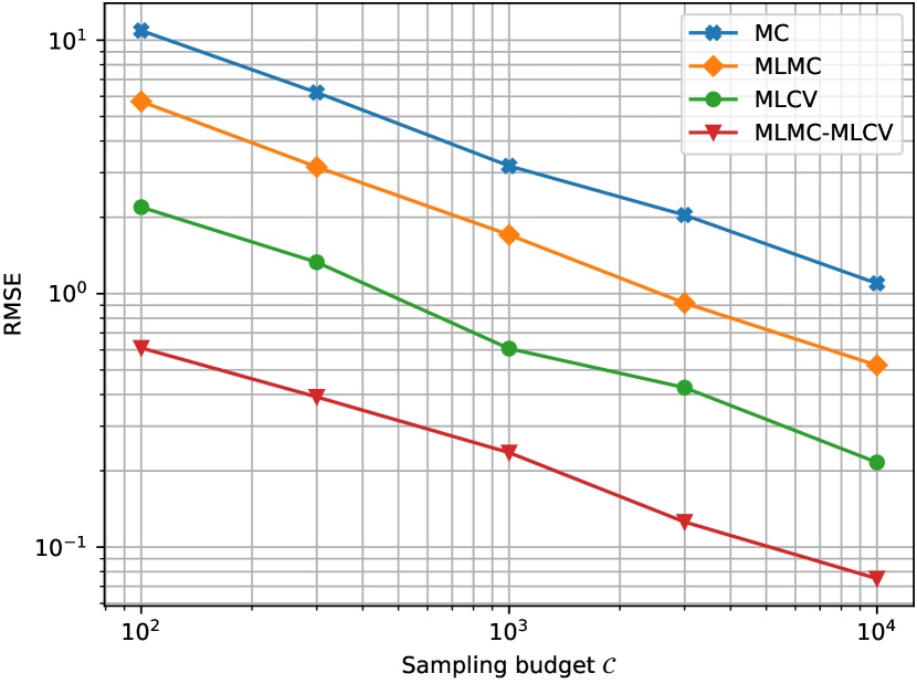
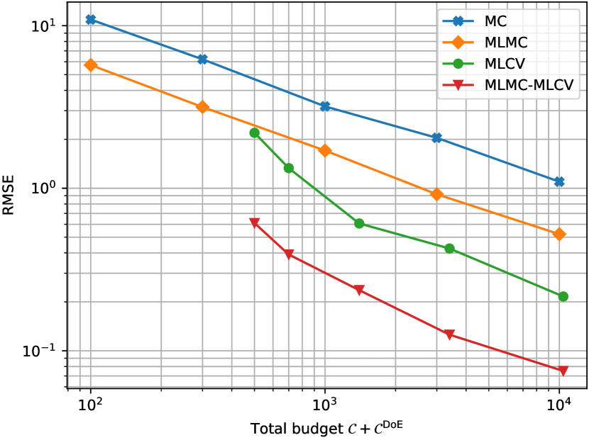
Figure 2(a) shows that, for a given sampling budget , the MC estimator is the least accurate. This can be explained by the fact that it only has access to the finest simulator, , whose cost only allows a limited number of evaluations. On the contrary, the MLMC estimator spreads this sampling budget over the four simulators. Ideally, the optimal sample allocation of MLMC eq. 60 results in many coarse, cheap evaluations and few fine, expensive evaluations. This is typically the case when the outputs of the simulators are highly correlated and the associated computational cost grows exponentially. Table 7 shows that the first assumption holds. The second assumption also holds since , being fixed, i.e., the evaluation cost grows linearly with the number of quadrature nodes. As a consequence, the MLMC estimator has a lower RMSE than the standard MC estimator.
| 1.00 | 0.96 | 0.97 | 0.93 | 0.80 | |
| 0.96 | 1.00 | 0.96 | 0.92 | 0.80 | |
| 0.97 | 0.96 | 1.00 | 0.95 | 0.81 | |
| 0.93 | 0.92 | 0.95 | 1.00 | 0.80 | |
| 0.80 | 0.96 | 0.81 | 0.80 | 1.00 |
For this experiment, the MLCV estimator is more accurate than the MLMC estimator. Based on one control variate per level , based on the PC model of from table 3, this estimator dedicates all the sampling budget to the finest simulator , and uses these control variates based on , , and to reduce the variance of the MC estimator at no extra cost, as the evaluation cost of a PC model is negligible compared to the evaluation cost of . This MLCV technique works particularly well in this case because the control variates are highly correlated to . Indeed, table 6 shows that their Pearson coefficients are at least 0.8, which guarantees a theoretical reduction of at least 94% in the variance of the MC estimator (i.e. a reduction of at least about 76% in standard deviation), corresponding to the variance reduction when using a single control variate based on . In fact, the variance reduction factor when using all the surrogates is only slightly higher, namely corresponding to a standard reduction factor of around 78%, which is reflected in fig. 2(a).
| 1.00 | 0.97 | 0.97 | 0.97 | -0.11 | -0.04 | -0.04 | 0.99 | 0.96 | 0.93 | 0.47 | -0.12 | -0.13 | -0.10 | |
| 0.97 | 1.00 | 1.00 | 1.00 | 0.13 | 0.19 | 0.19 | 0.97 | 0.97 | 0.93 | 0.48 | 0.12 | 0.09 | 0.09 | |
| 0.97 | 1.00 | 1.00 | 1.00 | 0.14 | 0.20 | 0.20 | 0.96 | 0.97 | 0.92 | 0.48 | 0.13 | 0.10 | 0.10 | |
| 0.97 | 1.00 | 1.00 | 1.00 | 0.14 | 0.20 | 0.20 | 0.96 | 0.97 | 0.92 | 0.48 | 0.13 | 0.10 | 0.10 | |
| -0.11 | 0.13 | 0.14 | 0.14 | 1.00 | 0.96 | 0.96 | -0.10 | 0.07 | 0.01 | 0.03 | 0.99 | 0.90 | 0.80 | |
| -0.04 | 0.19 | 0.20 | 0.20 | 0.96 | 1.00 | 1.00 | -0.03 | 0.12 | 0.06 | 0.06 | 0.94 | 0.90 | 0.81 | |
| -0.04 | 0.19 | 0.20 | 0.20 | 0.96 | 1.00 | 1.00 | -0.03 | 0.12 | 0.06 | 0.06 | 0.95 | 0.90 | 0.81 | |
| 0.99 | 0.97 | 0.96 | 0.96 | -0.10 | -0.03 | -0.03 | 1.00 | 0.96 | 0.93 | 0.48 | -0.11 | -0.12 | -0.09 | |
| 0.96 | 0.97 | 0.97 | 0.97 | 0.07 | 0.12 | 0.12 | 0.96 | 1.00 | 0.94 | 0.47 | 0.06 | 0.04 | 0.04 | |
| 0.93 | 0.93 | 0.92 | 0.92 | 0.01 | 0.06 | 0.06 | 0.93 | 0.94 | 1.00 | 0.47 | -0.00 | -0.03 | -0.02 | |
| 0.47 | 0.48 | 0.48 | 0.48 | 0.03 | 0.06 | 0.06 | 0.48 | 0.47 | 0.47 | 1.00 | 0.03 | 0.01 | 0.02 | |
| -0.12 | 0.12 | 0.13 | 0.13 | 0.99 | 0.94 | 0.95 | -0.11 | 0.06 | -0.00 | 0.03 | 1.00 | 0.91 | 0.80 | |
| -0.13 | 0.09 | 0.10 | 0.10 | 0.90 | 0.90 | 0.90 | -0.12 | 0.04 | -0.03 | 0.01 | 0.91 | 1.00 | 0.80 | |
| -0.10 | 0.09 | 0.10 | 0.10 | 0.80 | 0.81 | 0.81 | -0.09 | 0.04 | -0.02 | 0.02 | 0.80 | 0.80 | 1.00 |
Combining the MLMC and MLCV techniques allows the resulting MLMC-MLCV estimator to reduce the variance even more significantly. This can be explained by the very high correlation between , , and on the one hand, which ensures the good performance of the MLMC approach, and by the strong correlation between the control variates on the other hand, ensuring their good performance in combination with the MLMC technique. In particular, table 7 shows that , and are highly correlated with , with Pearson correlation coefficients greater than 0.9, while is poorly correlated with , with a correlation coefficient of 0.48. Besides, , and are well-correlated with , and , respectively, with correlation coefficients greater than 0.8.
Further insights regarding the expected variance reduction of the MLMC-MLCV estimator can be drawn from table 8, which reports the variance reduction factor w.r.t. pure MLMC on each level defined in eqs. 50 and 51, as well as the quantity defined in eq. 60. In particular, corresponds to the variance of the MLMC-MLCV estimator of the expectation with optimal sample allocation (see eq. 61), so that the ratio between the variance of MLMC-MLCV estimator and that of the MC estimator is (here with ). Furthermore, the variance of the different MLMC-based estimators per unit cost can be compared directly through . We observe that the variance of the MLMC-MLCV estimator is significantly reduced compared to that of the MLMC estimator, by about 98.6%, resulting in a reduction in standard deviation of about 88%. Again, this is well reflected in fig. 2(a).
| 0 | 1 | 2 | 3 | ||
| MLMC | 0 | 0 | 0 | 0 | |
| MLMC-CV | 0.9838 | 0.9916 | 0.8224 | 0.6469 | |
| MLMC-MLCV | 0.9840 | 0.9920 | 0.9173 | 0.9202 | |
| MLMC-CV[0] | 0.9838 | 0 | 0 | 0 | |
| MLMC-MLCV[0] | 0.9840 | 0.9916 | 0.8992 | 0.9027 | |
| MLMC | 69.63 % | 28.13 % | 1.68 % | 0.56 % | |
| MLMC-CV | 71.00 % | 20.66 % | 5.69 % | 2.66 % | |
| MLMC-MLCV | 73.66 % | 20.97 % | 4.05 % | 1.32 % | |
| MLMC-CV[0] | 22.59 % | 71.69 % | 4.29 % | 1.42 % | |
| MLMC-MLCV[0] | 72.84 % | 21.30 % | 4.42 % | 1.44 % | |
| MLMC | 1356.31 | 2673.54 | 2766.49 | 2797.65 | |
| MLMC-CV | 21.99 | 36.64 | 41.33 | 43.62 | |
| MLMC-MLCV | 21.72 | 35.85 | 38.99 | 40.04 | |
| MLMC-CV[0] | 21.99 | 382.87 | 418.54 | 430.71 | |
| MLMC-MLCV[0] | 21.76 | 36.35 | 39.84 | 41.01 | |
These first results from fig. 2(a) highlight the interest of multilevel control variates, be it with the MLMC-MLCV estimator or simply with the MLCV one. These results suppose that the PC models are not built specifically for the study, so that the budget does not include the number of -equivalent simulations required for their construction. Figure 2(b) illustrates the alternative case where the cost of the surrogate based CV estimators includes the cost of constructing the surrogates. As a result, an additional budget of (see section 4.2), is allocated to the construction of the PC models. As was the case for the single-level PC-based CV estimators, this results in an offset of 400 in the total cost of the MLCV and MLMC-MLCV estimators. The effect is especially noticeable when the construction budget larger than the estimation budget, i.e. for . For a sampling cost of 100, i.e. a total evaluation cost of 500, the MLCV estimator is still slightly more accurate than the MLMC estimator, while the MLMC-MLCV estimator still largely outperforms both.
4.3.3 Variants of MLMC-based CV estimators
The discussion about the surrogate construction budget prompts us to investigate variants of MLMC-MLCV using fewer surrogates, in order to reduce the total evaluation cost for limited budgets. The MLMC-CV estimator is described in section 3.2.2, while the variants MLMC-CV[0] and MLMC-MLCV[0] of MLMC-CV and MLMC-MLCV are introduced in table 1. The MLMC-CV[0] estimator only uses a control variate based on , so that the construction cost drops to , while the MLMC-MLCV[0] estimator uses control variates based on , and , so that the construction cost drops to . The MLMC-CV estimator uses control variates based on surrogates at all levels, so that the construction cost remains .
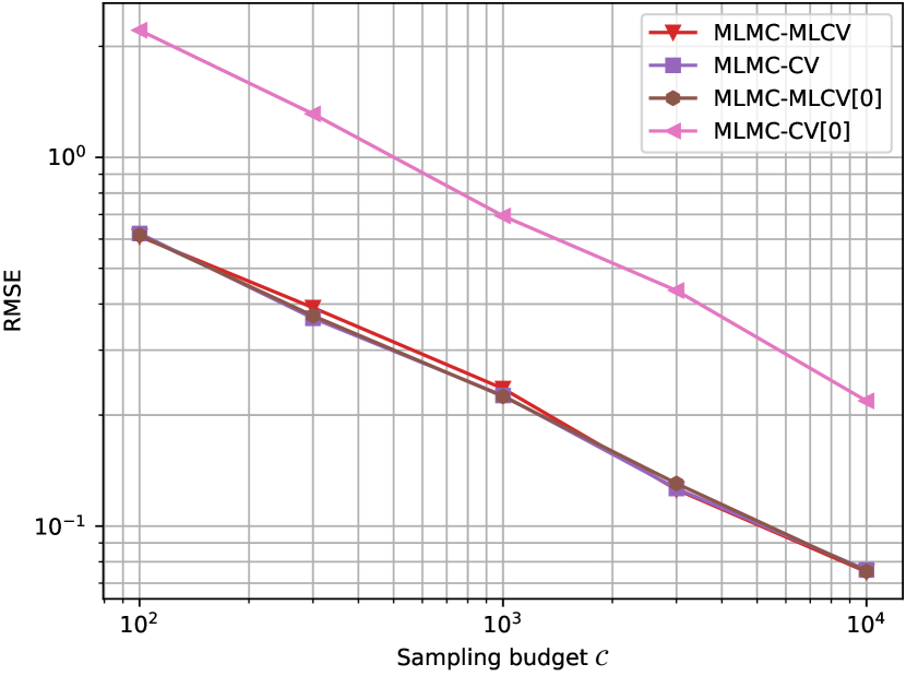
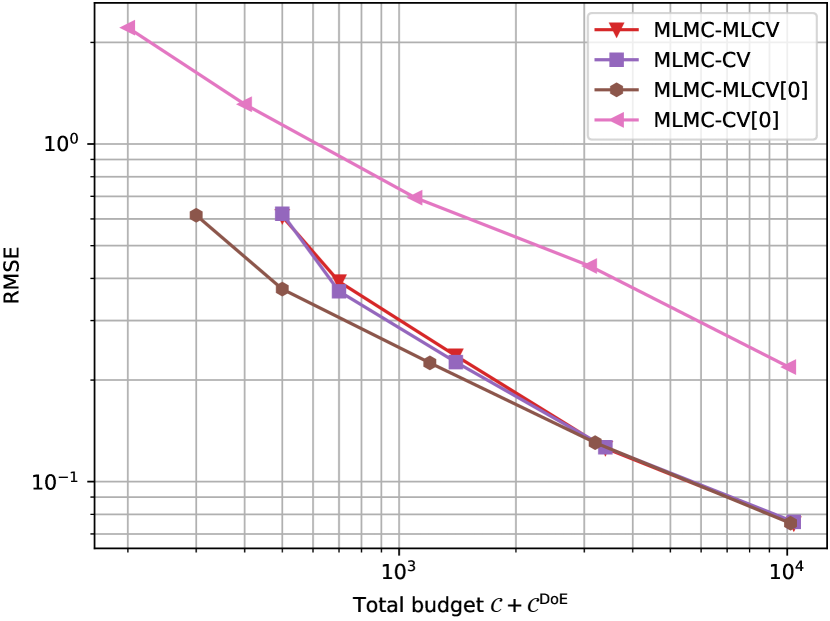
Figure 3(a) shows that MLMC-CV[0] has much higher RMSE than the other variants, resulting from the fact that it only reduces the variance associated with the coarsest level of the MLMC estimator. This behavior is consistent with the quantities of table 8. In particular, the value of is about 10 times higher than for the other variants, accounting for its RMSE being about 3 times higher than for the other variants. The remaining variants have similar performances regardless of the estimation budget, which is consistent with the values given in table 8. On the other hand, when considering the construction cost of the surrogates, fig. 3(b) shows that MLMC-MLCV[0] performs best, as it uses only surrogate models related to the two coarsest levels, namely , and , so that the construction cost is reduced. Furthermore, these surrogates have excellent , and they are such that is highly correlated with , is highly correlated with , and is highly correlated with , and . Namely, the associated Pearson correlation coefficients reported in table 7 are all at least 0.94. Therefore, should one have to build the surrogates specifically for the CV estimation of a statistic, it is more advantageous to adopt the MLMC-MLCV[0] variant over the others. In our case, the construction budget is divided by two compared to MLMC-MLCV and MLMC-CV, for a similar performance in terms of RMSE.
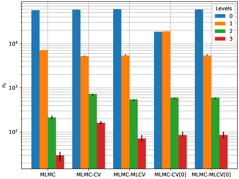
4.3.4 Budget allocation
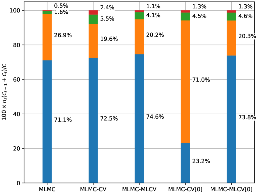
Lastly, fig. 4(a) shows the number of evaluations for each of the correction levels of the MLMC-* telescopic sum. Precisely, is the number of evaluations of , while is the number of evaluations of , for . We observe a typical sample allocation for MLMC-like estimators in ideal cases, that is, many coarse evaluations, and fewer and fewer fine evaluations. The MLMC-CV[0] estimator slightly deviates from this pattern, with , which can be explained by the fact that is of the same order of magnitude as . Figure 4(b) depicts the share of overall sampling cost associated with the different correction levels. Specifically, is the share of sampling budget dedicated to evaluating , and is the share dedicated to evaluating , for . We see that, except for MLMC-CV[0] for the reasons explained above, most of the sampling budget (around 70%) is allocated to the coarsest level, and most of the remaining budget is dedicated to correction level . We note that the CV-based MLMC estimators dedicate slightly more budget to levels 2 and 3 than for the standard MLMC estimator. The sampling budget shares of fig. 4(b) are consistent with the theoretical optimal shared reported in table 8, including those of the MLMC-CV[0] estimator. This suggests that the sample allocation resulting from algorithm 1 seems to converge to the theoretical optimal sample allocation eq. 60.
5 Conclusions
In this paper, we proposed multilevel variance reduction strategies relying on surrogate-based control variates. On the one hand, using specific surrogate models, such as polynomial chaos expansions or Taylor polynomial expansions, allows to directly access exact statistics (mean, variance) of the control variates. Even if these exactly statistics are not directly accessible (e.g., when using GPs), they can be estimated very accurately at negligible cost. This contrasts with typical control variates relying on lower-fidelity models based on models/simulators with degraded physics or coarser discretizations, for which approximate control variate strategies need to be devised, resulting in a lower variance reduction. On the other hand, when multiple levels of fidelities (e.g., based on the discretization) with a clear cost/accuracy hierarchy are available, the surrogate-based control variate approach can be efficiently combined with multilevel strategies. The first strategy, MLCV, simply consists in using multiple control variates based on surrogate models of the simulators corresponding to the different levels. The main advantage is that the surrogate models corresponding to coarse levels may be constructed using larger sample sizes than for the finest level, resulting in a more accurate surrogate model (i.e., with lower model error). This strategy thus leads to a greater variance reduction compared to only using one surrogate model based on the finest level. This is supported by the numerical experiments we conducted, as well as by the theoretical variance reduction provided by proposition 1. The second strategy, MLMC-MLCV, allows to further improve the variance reduction by combining the surrogate-based control variates with an MLMC strategy. The most appropriate way to construct and utilize the surrogate models is, however, not straightforward, and was discussed in detail in sections 3.2.2 and 3.2.3. The additional variance reduction as compared to plain MLMC is demonstrated in our numerical experiments and supported by the theoretical variance reduction factor eq. 51 derived in section 3.2.3.
The construction cost of the surrogate models was discussed from two perspectives. When the surrogate models are constructed for the sole purpose of serving for the control variate estimation, then the cost of their construction must be taken into account for fair comparison with other approaches. In such a case, it may not be optimal, in terms of cost/accuracy tradeoff, to construct surrogate models on all levels, especially when only a limited budget is available. In particular, using a subset of surrogate models based on the coarser levels may already lead to considerable variance reduction, provided that the outputs of the coarse surrogate models are sufficiently correlated with that of the high-fidelity simulator. Then, considering additional surrogate models on finer levels might only result in marginal improvement, at the expense of a significant computational cost. On the contrary, if the surrogate models have already been constructed for other purposes, and are, in some sense, available “for free,” then their construction cost need not be considered, and the entire set of surrogate models may then be used.
From the former perspective, that is when the cost of the surrogate construction is considered as part of the estimation cost, one may devise more involved strategies seeking to optimize the tradeoff between the construction cost and the model error, directly impacting the projected variance reduction. For instance, in the context of polynomial chaos surrogate models, the truncation strategy may be controlled to this end, as proposed in a stochastic Galerkin framework in [56], where the total polynomial degree is optimized alongside the sample size and the CV parameter to minimize the PC-based CV estimator’s variance under a cost constraint. Another avenue to improve the proposed approach would be to replace the MLMC part of the MLMC-MLCV strategy by a more efficient multilevel approach, such as the multilevel best linear unbiased estimator (MLBLUE) [48, 49, 47]. In particular, an MLBLUE-MLCV strategy should be more efficient when a collection of low-fidelity simulators (e.g., with degraded physics) with no clear cost/accuracy hierarchy is available. Finally, although the proposed approaches apply to the estimation of arbitrary statistics, they were only tested here on the estimation of expected values. The theoretical and algorithmic ingredients for the estimation of variances are, however, described in this paper and may be tested in follow-up investigations and numerical experiments. Specifically, the multifidelity estimation of variance-based sensitivity indices is of particular interest to our team.
6 Acknowledgment
We wish to acknowledge the PIA framework (CGI, ANR) and the industrial members of the IRT Saint Exupéry project R-Evol: Airbus, Liebherr, Altran Technologies, Capgemini DEMS France, CENAERO and Cerfacs for their support, financial funding and own knowledge.
Appendix A Optimal parameter for expectation and variance CV estimators
We derive here the expression of the optimal CV parameter for the CV estimators of the expectation and of the variance. We define , and . Then, given an input -sample , we define , and .
A.1 CV estimator of the expectation
For the expectation, we have and , i.e.
| (78) | ||||
| (79) |
so that , , and, eventually,
| (80) |
Furthermore, we have , so that
| (81) |
where
| (82) |
Thus, corresponds to the squared coefficient of multiple correlation between and the control variates .
A.2 CV estimator of the variance
Similarly, for the variance, we have and . We start by deriving useful identities. In what follows, for any random variable , we denote the corresponding centered variable by . First, we remark that , so that, for any two random variables and ,
| (83) |
Furthermore, it can be shown that
| (84) |
with (see proof below)
| (85) | ||||
| (86) | ||||
| (87) |
We thus have
| (88) | ||||
| (89) |
eventually leading to
| (90) | ||||
| (91) |
so that
| (92) | ||||
| (93) |
As , we see that
| (94) | ||||
| (95) |
where
| (96) |
with . Thus, corresponds to the squared coefficient of multiple correlation between and .
We now proceed to the proof of identities eqs. 85, 86, and 87. First, for eq. 85, by definition
| (97) |
We distinguish two (disjoint) cases:
-
1.
: . There are such terms in the sum.
-
2.
: . There are such terms in the sum.
Then eq. 85 follows. For eq. 86,
| (98) |
We distinguish five (disjoint) cases:
-
1.
: . There are such terms in the sum.
-
2.
: . There are such terms in the sum.
-
3.
: . There are such terms in the sum.
-
4.
: . There are such terms in the sum.
-
5.
All remaining cases (at least one of the indices is different from all the others): .
Then eq. 86 follows. Finally, for eq. 87,
| (99) |
We distinguish three (disjoint) cases:
-
1.
: . There are such terms in the sum.
-
2.
: . There are such terms in the sum.
-
3.
All remaining cases (at least one of the indices is different from all the others): .
Then eq. 87 follows.
Remark 4.
When the expected value of is known, as is the case when defining from the prediction of certain surrogate models, such as PC exansion and Taylor polynomials (and, in some instances, GPs, see section 2.4.1), it is possible to replace with . The derivation of the optimal CV parameter is somewhat easier and leads to similar results as in the unknown expectation case. Specifically,
| (100) | ||||
| (101) | ||||
| (102) |
i.e. . Regarding the vector of covariances ,
| (103) | ||||
| (104) | ||||
| (105) | ||||
| (106) |
i.e. , so that
| (107) | ||||
| (108) |
with the same definitions as in eq. 95.
Appendix B Optimal MLMC-MLCV variance estimator
The MLMC-MLCV variance estimator is given by eq. 45, with
| (109) | ||||
| (110) |
where
| (111) | ||||||
| (112) | ||||||
| (113) | ||||||
| (114) | ||||||
Furthermore, we assume that the expected values of the control variates are known, so that we use the following variance estimators:
| (115) |
The optimal values of the CV parameters are given by
| (116) | ||||||||
| (117) |
Note that is the same for all . For PC-based control variates, and , letting , we have
| (118) |
where for and for . Consequently,
| (119) | ||||||
| (120) |
Furthermore,
| (121) |
where are the entries of the fourth-order Galerkin product tensor, which is a well-known object in stochastic Galerkin methods [20, 32], and denotes the Kronecker delta. Besides, noticing that , with and the definitions in eq. 55, we have
| (122) |
where
| (123) | ||||
| (124) | ||||
| (125) | ||||
| (126) | ||||
| (127) | ||||
| (128) |
Appendix C Taylor surrogate for the numerical test case
In our example, is only differentiable in . Consequently, the Taylor polynomial surrogate cannot be used directly as defined in (17) and (18), because the Jacobian and Hessian matrices are not defined at . Instead, we define the first-order Taylor surrogate as
| (129) |
where, for , , and, for ,
| (130) |
where , which is now well-defined.
With our choice of distributions for given in (72), we have , and the first-order Taylor surrogate is defined by (129), with
| (131) | ||||
| (132) | ||||
| (133) | ||||
| (134) | ||||
| (135) | ||||
| (136) | ||||
| (137) |
Because of the piecewise definition of , the identity for a regular first-order Taylor surrogate no longer holds. Instead, we have
| (138) |
References
- [1] T. W. Anderson, An Introduction to Multivariate Statistical Analysis, Wiley Series in Probability and Statistics, Wiley-Interscience, Hoboken, N.J, 3rd ed ed., 2003.
- [2] I. Babuška, F. Nobile, and R. Tempone, A Stochastic Collocation Method for Elliptic Partial Differential Equations with Random Input Data, SIAM Journal on Numerical Analysis, 45 (2007), pp. 1005–1034.
- [3] M. Berveiller, B. Sudret, and M. Lemaire, Stochastic finite element: A non intrusive approach by regression, European Journal of Computational Mechanics, 15 (2006), pp. 81–92.
- [4] C. Bierig and A. Chernov, Convergence analysis of multilevel Monte Carlo variance estimators and application for random obstacle problems, Numerische Mathematik, 130 (2015), pp. 579–613.
- [5] , Estimation of arbitrary order central statistical moments by the multilevel Monte Carlo method, Stochastics and Partial Differential Equations Analysis and Computations, 4 (2016), pp. 3–40.
- [6] G. Blatman and B. Sudret, Efficient computation of global sensitivity indices using sparse polynomial chaos expansions, Reliability Engineering & System Safety, 95 (2010), pp. 1216–1229.
- [7] , Adaptive sparse polynomial chaos expansion based on least angle regression, Journal of Computational Physics, 230 (2011), pp. 2345–2367.
- [8] F.-X. Briol, C. J. Oates, M. Girolami, M. A. Osborne, and D. Sejdinovic, Probabilistic Integration: A Role in Statistical Computation?, Statistical Science, 34 (2019), pp. 1–22.
- [9] R. H. Cameron and W. T. Martin, The orthogonal development of non-linear functionals in series of Fourier-Hermite functionals, Annals of Mathematics, 48 (1947), pp. 385–392.
- [10] K. A. Cliffe, M. B. Giles, R. Scheichl, and A. L. Teckentrup, Multilevel Monte Carlo methods and applications to elliptic PDEs with random coefficients, Computing and Visualization in Science, 14 (2011), pp. 3–15.
- [11] P. R. Conrad and Y. M. Marzouk, Adaptive Smolyak Pseudospectral Approximations, SIAM Journal on Scientific Computing, 35 (2013), pp. A2643–A2670.
- [12] P. G. Constantine, M. S. Eldred, and E. T. Phipps, Sparse pseudospectral approximation method, Computer Methods in Applied Mechanics and Engineering, 229–232 (2012), pp. 1–12.
- [13] J. Dick, F. Y. Kuo, and I. H. Sloan, High-dimensional integration: The quasi-monte carlo way, Acta Numerica, 22 (2013), p. 133–288.
- [14] B. Efron, T. Hastie, I. Johnstone, and R. Tibshirani, Least Angle Regression, The Annals of Statistics, 32 (2004), pp. 407–451.
- [15] R. EL Amri, R. Le Riche, C. Helbert, C. Blanchet-Scalliet, and S. Da Veiga, A sampling criterion for constrained bayesian optimization with uncertainties, arXiv preprint arXiv:2103.05706, (2021).
- [16] J. Fox and G. Ökten, Polynomial chaos as a control variate method, SIAM Journal on Scientific Computing, 43 (2021), pp. A2268–A2294.
- [17] S. Garg, N. Sood, and C. D. Sarris, Uncertainty quantification of ray-tracing based wireless propagation models with a control variate-polynomial chaos expansion method, in 2015 IEEE International Symposium on Antennas and Propagation & USNC/URSI National Radio Science Meeting, 2015, pp. 1776–1777.
- [18] G. Geraci, M. Eldred, and G. Iaccarino, A multifidelity control variate approach for the multilevel Monte Carlo technique, tech. rep., Stanford University, 2015.
- [19] G. Geraci, M. S. Eldred, and G. Iaccarino, A multifidelity multilevel Monte Carlo method for uncertainty propagation in aerospace applications, in 19th AIAA Non-Deterministic Approaches Conference, Grapevine, Texas, 2017, American Institute of Aeronautics and Astronautics.
- [20] R. G. Ghanem and P. D. Spanos, Stochastic Finite Elements: A Spectral Approach, Courier Corporation, 2003.
- [21] M. B. Giles, Multilevel Monte Carlo Path Simulation, Operations Research, 56 (2008), pp. 607–617.
- [22] , Multilevel Monte Carlo methods, Acta Numerica, 24 (2015), pp. 259–328.
- [23] M. B. Giles and B. J. Waterhouse, Multilevel quasi-Monte Carlo path simulation, Advanced Financial Modelling, Radon Series on Computational and Applied Mathematics, 8 (2009), pp. 165–181.
- [24] A. A. Gorodetsky, G. Geraci, M. S. Eldred, and J. D. Jakeman, A generalized approximate control variate framework for multifidelity uncertainty quantification, Journal of Computational Physics, 408 (2020), p. 109257.
- [25] Z. Gu and C. D. Sarris, Multi-parametric uncertainty quantification with a hybrid monte-carlo / polynomial chaos expansion fdtd method, in 2015 IEEE MTT-S International Microwave Symposium, 2015, pp. 1–3.
- [26] A.-L. Haji-Ali, F. Nobile, and R. Tempone, Multi-index Monte Carlo: When sparsity meets sampling, Numerische Mathematik, 132 (2016), pp. 767–806.
- [27] T. Hesterberg, Weighted average importance sampling and defensive mixture distributions, Technometrics, 37 (1995), pp. 185–194.
- [28] J. Janusevskis and R. Le Riche, Simultaneous kriging-based estimation and optimization of mean response, Journal of Global Optimization, 55 (2013), pp. 313–336.
- [29] S. S. Lavenberg, T. L. Moeller, and P. D. Welch, The application of control variables to the simulation of closed queueing networks, in Proceedings of the 9th Conference on Winter Simulation - Volume 1, WSC ’77, Gaitherburg, Maryland, USA, 1977, Winter Simulation Conference, pp. 152–154.
- [30] S. S. Lavenberg, T. L. Moeller, and P. D. Welch, Statistical Results on Control Variables with Application to Queueing Network Simulation, Operations Research, 30 (1982), pp. 182–202.
- [31] S. S. Lavenberg and P. D. Welch, A Perspective on the Use of Control Variables to Increase the Efficiency of Monte Carlo Simulations, Management Science, 27 (1981), pp. 322–335.
- [32] O. P. Le Maître and O. M. Knio, Spectral Methods for Uncertainty Quantification, Scientific Computation, Springer Netherlands, Dordrecht, 2010.
- [33] C. Lemieux, Control Variates, in Wiley StatsRef: Statistics Reference Online, American Cancer Society, 2017, pp. 1–8.
- [34] N. Lüthen, S. Marelli, and B. Sudret, Sparse polynomial chaos expansions: Literature survey and benchmark, SIAM/ASA Journal on Uncertainty Quantification, 9 (2021), pp. 593–649.
- [35] M. McKay, R. Beckman, and W. Conover, Acomparisonof three methods for selecting values of input variables in the analysis of output from a computer code, Technometrics, 21 (1979), pp. 239–245.
- [36] P. Mycek and M. De Lozzo, Multilevel Monte Carlo Covariance Estimation for the Computation of Sobol’ Indices, SIAM/ASA Journal on Uncertainty Quantification, 7 (2019), pp. 1323–1348.
- [37] H. N. Najm, Uncertainty quantification and polynomial chaos techniques in computational fluid dynamics, Annual Review of Fluid Mechanics, 41 (2009), pp. 35–52.
- [38] B. L. Nelson, Control Variate Remedies, Operations Research, 38 (1990), pp. 974–992.
- [39] L. W. T. Ng and K. E. Willcox, Multifidelity approaches for optimization under uncertainty, International Journal for Numerical Methods in Engineering, 100 (2014), pp. 746–772.
- [40] F. Nobile, R. Tempone, and C. G. Webster, An Anisotropic Sparse Grid Stochastic Collocation Method for Partial Differential Equations with Random Input Data, SIAM Journal on Numerical Analysis, 46 (2008), pp. 2411–2442.
- [41] J. Park and I. W. Sandberg, Universal Approximation Using Radial-Basis-Function Networks, Neural Computation, 3 (1991), pp. 246–257.
- [42] R. Pasupathy, B. W. Schmeiser, M. R. Taaffe, and J. Wang, Control-variate estimation using estimated control means, IIE Transactions, 44 (2012), pp. 381–385.
- [43] B. Peherstorfer, K. Willcox, and M. Gunzburger, Optimal Model Management for Multifidelity Monte Carlo Estimation, SIAM Journal on Scientific Computing, 38 (2016), pp. A3163–A3194.
- [44] , Survey of Multifidelity Methods in Uncertainty Propagation, Inference, and Optimization, SIAM Review, 60 (2018), pp. 550–591.
- [45] C. E. Rasmussen, Gaussian Processes in Machine Learning, Springer Berlin Heidelberg, Berlin, Heidelberg, 2004, pp. 63–71.
- [46] M. T. Reagan, H. N. Najm, R. G. Ghanem, and O. M. Knio, Uncertainty quantification in reacting-flow simulations through non-intrusive spectral projection, Combustion and Flame, 132 (2003), pp. 545–555.
- [47] D. Schaden, Variance Reduction with Multilevel Estimators, PhD thesis, Technische Universität München, Munich, 2021.
- [48] D. Schaden and E. Ullmann, On Multilevel Best Linear Unbiased Estimators, SIAM/ASA Journal on Uncertainty Quantification, 8 (2020), pp. 601–635.
- [49] , Asymptotic Analysis of Multilevel Best Linear Unbiased Estimators, SIAM/ASA Journal on Uncertainty Quantification, 9 (2021), pp. 953–978.
- [50] R. C. Smith, Uncertainty Quantification: Theory, Implementation, and Applications, Society for Industrial and Applied Mathematics, USA, 2013.
- [51] B. Sudret, Global sensitivity analysis using polynomial chaos expansions, Reliability Engineering & System Safety, 93 (2008), pp. 964–979.
- [52] T. J. Sullivan, Introduction to Uncertainty Quantification, vol. 63, Springer Cham, 2015.
- [53] A. L. Teckentrup, Multilevel Monte Carlo Methods and Uncertainty Quantification, PhD thesis, University of Bath, 2013.
- [54] R. K. Tripathy and I. Bilionis, Deep uq: Learning deep neural network surrogate models for high dimensional uncertainty quantification, Journal of Computational Physics, 375 (2018), pp. 565–588.
- [55] N. Wiener, The Homogeneous Chaos, American Journal of Mathematics, 60 (1938), pp. 897–936.
- [56] H. Yang, Y. Fujii, K. W. Wang, and A. A. Gorodetsky, Control Variate Polynomial Chaos: Optimal Fusion of Sampling and Surrogates for Multifidelity Uncertainty Quantification, arXiv:2201.10745 [stat], (2022).