On the Number of components of random polynomial lemniscates

Abstract.

A lemniscate of a complex polynomial $Q_{n}$ of degree $n$ is a sublevel set of its modulus, i.e., of the form $\{z\in\mathbb{C}:|Q_{n}(z)|<t\}$ for some $t>0.$ In general, the number of connected components of this lemniscate can vary anywhere between 1 and $n$. In this paper, we study the expected number of connected components for two models of random lemniscates. First, we show that lemniscates whose defining polynomial has i.i.d. roots chosen uniformly from $\mathbb{D}$, has on average $\mathcal{O}(\sqrt{n})$ number of connected components. On the other hand if the i.i.d. roots are chosen uniformly from $\mathbb{S}^{1}$, we show that the expected number of connected components, divided by n, converges to $\frac{1}{2}$.

1. Introduction

Let $Q_{n}(z)$ be a monic polynomial of degree $n$ in the complex plane such that all its roots are contained within the closed unit disk $\overline{\mathbb{D}}$. That is,

$$Q_{n}(z):=\prod_{i=1}^{n}(z-z_{i}),$$ (1)

where $|z_{j}|\leq 1$, for $1\leq j\leq n$. We denote the unit lemniscate of $Q_{n}(z)$ by $\Lambda(Q_{n}):=\{z\in\mathbb{C}:|Q_{n}(z)|<1\}.$ The quantity of interest is the number of connected components of $\Lambda$. The maximum principle implies that each connected component of the lemniscate must contain a zero of the polynomial; therefore, there are at most $n$ components. In this paper, we investigate the number of components of a typical lemniscate. Numerical simulations for random polynomials with roots chosen from the uniform probability measure on the unit disk $\mathbb{D}$, and on the circle $\mathbb{S}^{1}$ show a giant component alongside some tiny components (see Figures 1, 2). In this paper, we quantify this numerical observation.

1.1. Motivation and Previous Results

The study of the metric and topological properties of polynomial lemniscates serves two main purposes. Firstly, it is the simplest curve with an algebraic boundary that is relevant to many problems in mathematical physics [19, 5, 2]. Secondly, polynomial lemniscates are used as a tool for approximating and analyzing complex geometric objects due to implications of Hilbert’s lemniscate Theorem and its generalizations [28, 24]. For a more detailed exposition, please refer to [20] and the corresponding references therein. Taking all these into account, in 1958, Erdős, Herzog, and Piranian in [9] studied the geometric and topological properties of polynomial lemniscates and posed a long list of open problems. One of the key motivations behind the work related to random polynomial lemniscates is to offer a probabilistic approach to the problems in [9]. Krishnapur, Lundberg, and Ramachandran recently showed that the inradius of a random lemniscate whose defining polynomial has roots chosen from a measure $\mu$ depends on the negative set of the logarithmic potential $U_{\mu}$. Lundberg, Epstein, and Hanin conducted a study on the lemniscate tree that encodes the nesting structure of the level sets of a random polynomial in [8]. Lundberg and Ramachandran in [22] conducted a study on the Kac ensemble and found that the expected number of connected components is asymptotically $n$. Lerario and Lundberg [21] proved that for random rational lemniscates, which are defined as the quotient of two spherical random polynomials, the average number of connected components is $\mathcal{O}(n)$. Later, Kabluchko and Wigman [18] discovered the exact asymptotics. Fyodorov, Lerario, and Lundberg studied the number of connected components of random algebraic hypersurfaces in [10]. In this article, we examine random polynomials with random roots, in contrast to random coefficients. Another stream of research on random polynomials includes studying the roots and critical points of random polynomials. In this work, we have made use of one such pairing result due to Kabluchko and Seidel [17], which states that for random polynomials whose roots are sampled from an appropriate probability measure $\nu$ supported within the unit disk, each root is associated with a critical point in close proximity. For more background, details and generalizations consult [13], [26], [16], [30], [27], [4], [23], [1], [14], [15], [25]. To find related research on meromorphic functions and Gaussian polynomials, please refer to [12], [11]. We emphasize the fact that such pairing phenomena are exclusive to random polynomials. The analogous result in the deterministic setting is Sendov’s conjecture [29], which was recently proven by Tao in [31] for all polynomials of sufficiently large degree.

1.2. Main Results

In all the theorems we have the following setting.

Setting and notations: Let $\{X_{i}\}_{i=1}^{\infty}$ be a sequence of i.i.d. random variables with law $\mu$, supported in the closed unit disk. Consider the sequence of random polynomials defined by

$$P_{n}(z):=\prod_{i=1}^{n}(z-X_{i})$$ (2)

and its lemniscate

$$\Lambda_{n}:=\Lambda(P_{n})=\{z\in\mathbb{C}:|P_{n}(z)|<1\}.$$

We denote by $C(\Lambda_{n})$ the number of connected components of the lemniscate $\Lambda_{n}$. Throughout the paper, we denote by C a positive numerical constant whose values may vary from line to line. For a set $S\subset\mathbb{C}$, we denote by $|S|$ the cardinality of the set $S$. The following are the main theorems of this paper.

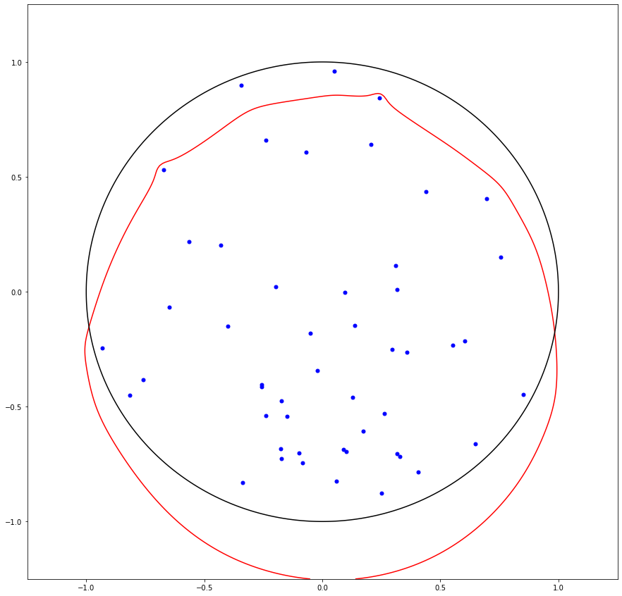
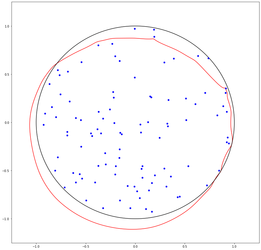
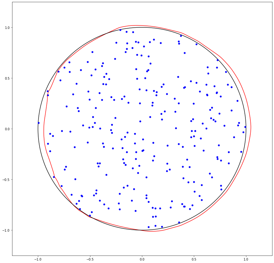
Figure 1. Lemniscates of degree n = 50, 100, 250 with zeros sampled uniformly from the open unit disk.

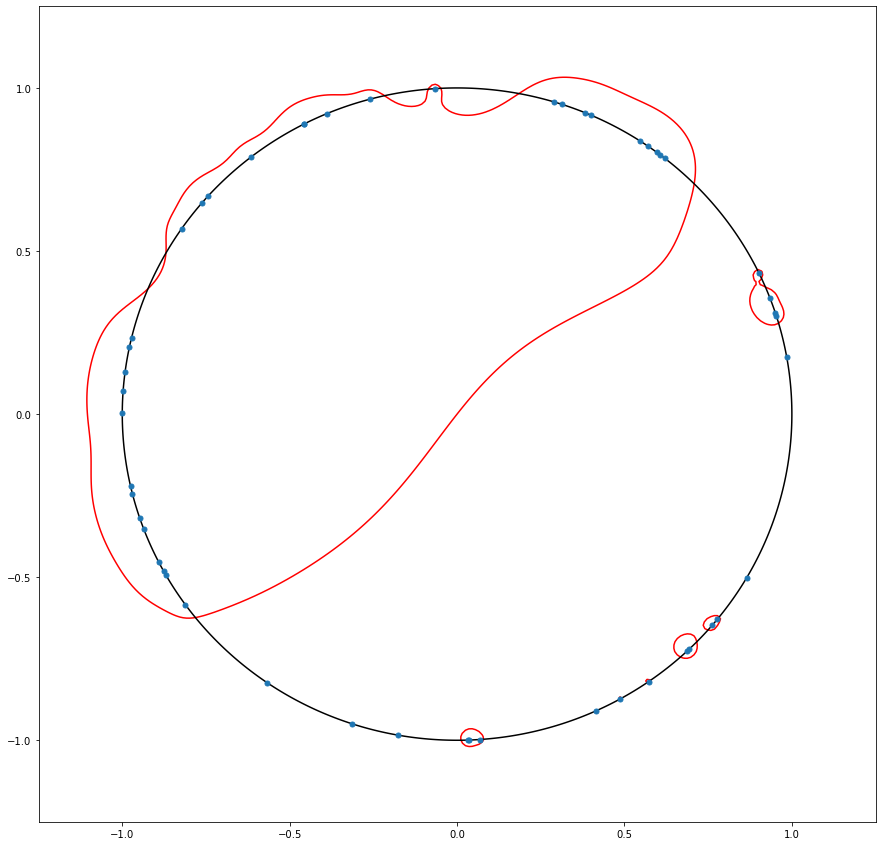
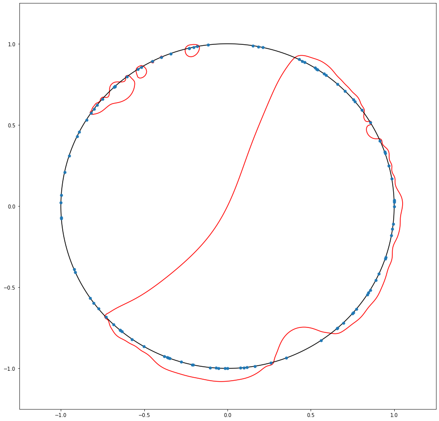
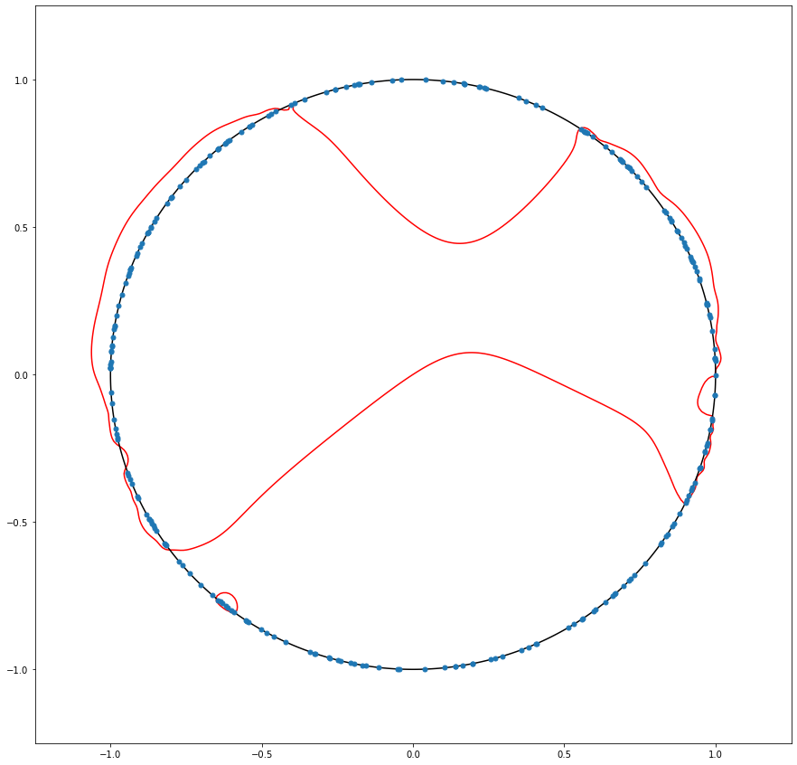
Figure 2. Lemniscates of degree n = 50, 100, 250 with zeros sampled uniformly from the unit circle. A unit circle is also plotted for reference in each case.

Theorem 1.1.

Let $\mu$ be the probability measure distributed uniformly in the unit disk $\mathbb{D}$. Then there exist absolute constants $C_{1},C_{2}>0$ such that for all large $n$ we have

$$C_{1}\sqrt{n}\leq{\mathbb{E}[C(\Lambda_{n})]}\leq C_{2}\sqrt{n}.$$

Theorem 1.2.

Let $\mu$ be the probability measure distributed uniformly in the unit circle $\mathbb{S}^{1}$. Then

$$\lim_{n\to\infty}\frac{\mathbb{E}[C(\Lambda_{n})]}{n}=\frac{1}{2}.$$

1.3. Remarks

What happens if we choose $\mu$ to be the uniform measure on $r\mathbb{D}$ or $r\mathbb{S}^{1}$? Let us consider the uniform probability measure on $r\mathbb{S}^{1}$ say $\mu_{r}$. Then it is easy to show that the logarithmic potential is

$$U_{\mu_{r}}(z)=\begin{cases}\log|z|&\mbox{ if }|z|\geq r,\\ \log r&\mbox{ if }|z|<r.\end{cases}$$ (3)

Case 1 $(r<1)$:

In this case, the potential (3) is negative in the whole unit disk. Therefore the set $r\mathbb{D}$ is enclosed within the lemniscate by Theorem 1.1 in [20], resulting in a single connected component with overwhelming probability.

Case 2 $(r>1)$:

In this case, the potential (3) is positive in the entire complex plane therefore we get with overwhelming probability, $n$ components for the lemniscate, by the implications of Theorem 1.3 of [20].

So in some sense, $r=1$ is the critical case in this model. A similar analysis for the uniform probability measure on $r\mathbb{D}$ is done in [20], example-1.7. See Figure 3, 4. The above results and the results in this paper are summarized schematically in Table 1.

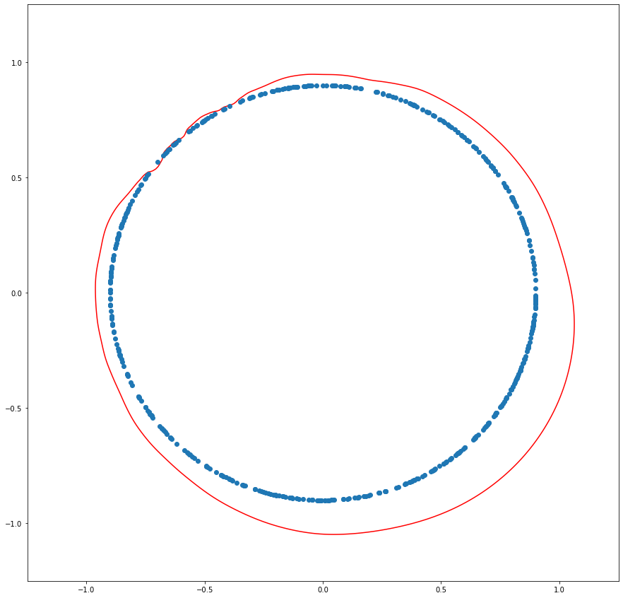
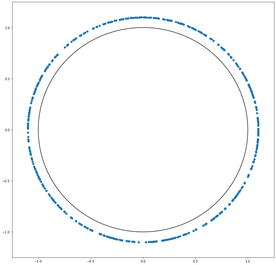
Figure 3. Lemniscates of degree n = 500 with zeros sampled uniformly from $r\mathbb{S}^{1}$, for $r=0.9$ and $1.1$ respectively.

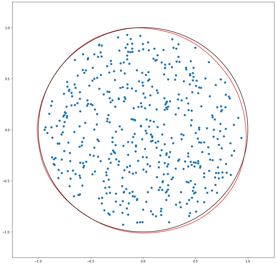
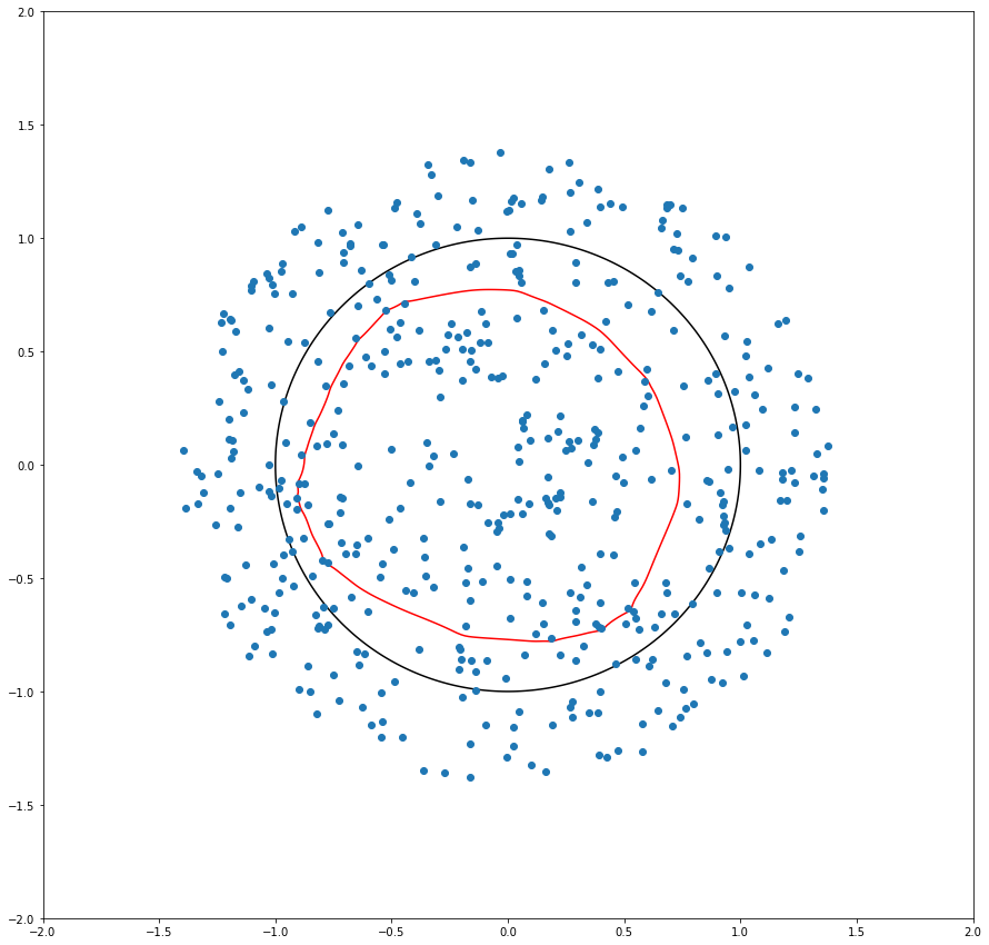
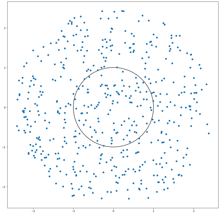
Figure 4. Lemniscates of degree n = 500 with zeros sampled uniformly from $r\mathbb{D}$ for $r=0.95,0.85\sqrt{e},$ and $1.5\sqrt{e}$ respectively.

	$\boldsymbol{\mu}$	$\mathbf{r<1}$	$\mathbf{r=1}$	$\mathbf{\sqrt{e}\geq r>1}$	$\mathbf{r>1}$
$\boldsymbol{\mathbb{E}[C(\Lambda_{n})]}$	Uniform probability measure in $r\mathbb{D}$	$1$	$\mathcal{O}(\sqrt{n})$	$C_{r}n$	$n$
$\boldsymbol{\mathbb{E}[C(\Lambda_{n})]}$	Uniform probability measure in $r\mathbb{S}^{1}$	$1$	$\frac{n}{2}$	$n$	$n$

Table 1. Asymptotics of Expected No. of Components for Different Values of $r$.

1.4. Heuristics and ideas of proof

We will now provide an overview of the underlying heuristics behind our results. In the first model, which involves random polynomials with uniformly chosen roots from $\mathbb{D}$, the potential $U_{\mu}(z)$ is negative throughout the unit disk. By writing $\log|P_{n}(z)|=\sum_{i=1}^{n}\log|z-X_{i}|$ as the sum of independent random variables with mean $U_{\mu}(z)$, we employ various concentration estimates to analyze the behavior of $|P_{n}(z)|$. Since the sum of i.i.d. random variables concentrate near its mean which is negative, most of the region within the disk, away from the boundary, lies inside the lemniscate. It is only near the boundary, where the potential approaches zero, isolated components are formed due to the fluctuations governed by the Central Limit Theorem, resulting in $\mathcal{O}(\sqrt{n})$ many components. In the other model, i.e., random polynomial with roots chosen uniformly on the circle, the potential is zero in the whole disk. The probability of any point on $\mathbb{S}^{1}$ being inside the lemniscate is close to $\frac{1}{2}$. Therefore, if we start with $P_{n}$ and introduce a new root $X_{n+1}$ to build $P_{n+1},$ $X_{n+1}$ will land outside $\Lambda_{n}$ with probability approximately $\frac{1}{2}$, forming an isolated component. Therefore, on average, we get approximately $\frac{n}{2}$ components. In both models, we establish the lower bound by estimating the number of isolated components. To determine the upper bound for the disk case, we utilize an analytical characterization for the number of components (see Lemma 2.8), which asserts that the number of components is one more than the number of critical points whose critical value is larger or equal to $1$. To determine the number of such critical points, we employ a pairing result from [17] to associate critical points with roots with some desired properties. The number of such roots yields the desired upper bound. However, in the other case, the pairing phenomena does not occur. There we establish the upper bound by showing that the number of components possessing fewer than $n^{\varepsilon}$ roots, when divided by $n$, tends towards $\frac{1}{2}$, for sufficiently small $\varepsilon$.

2. Preliminary Lemmas

Before delving into the proofs of the main theorems, we gather preliminary theorems and lemmas that are utilized repeatedly in both theorems.

Theorem 2.1.

(Berry-Esseen) Let $X_{1},X_{2},...$ be i.i.d. random variables with $\mathbb{E}X_{i}=0,\mathbb{E}X_{i}^{2}=\sigma^{2},$ and $\mathbb{E}|X_{i}|^{3}=\rho<\infty.$ If $F_{n}(x)$ is the distribution function of $\frac{(X_{1}+...+X_{n})}{\sigma\sqrt{n}}$ and $\Phi(x)$ is the standard normal distribution, then

$$|F_{n}(x)-\Phi(x)|\leq\frac{3\rho}{\sigma^{3}\sqrt{n}}.$$ (4)

The proof of Theorem 2.1 can be found in [7] Theorem 3.4.17.

Theorem 2.2.

[Bennett’s inequality] Let $Y_{1},Y_{2},...,Y_{n}$ be independent random variables with finite variance such that $\forall$ $i\leq n$, $Y_{i}\leq b$, for some $b>0$ almost surely. Let

$$S=\sum_{i=1}^{n}\left(Y_{i}-\mathbb{E}[Y_{i}]\right),$$

and $\nu=\sum_{i=1}^{n}\mathbb{E}[{Y_{i}}^{2}].$ Then for any $t>0,$ we have

$$\mathbb{P}(S>t)\leq\exp\left(-\frac{\nu}{b^{2}}h\Big{(}\frac{bt}{\nu}\Big{)}\right),$$

where $h(u)=(1+u)\log(1+u)-u\textit{, for }u>0.$

For the proof of this concentration inequality and other similar results see [3].

Lemma 2.3.

Let $X$ be a random variable taking values in $\overline{\mathbb{D}}$ with law $\mu$. Assume that for all $z\in\mathbb{D},r\leq 2$, there exist constants $\varepsilon,M_{1},M_{2}\in(0,\infty)$ such that $\mu$ satisfies

$$M_{1}r^{\varepsilon}\leq\mu(B(z,r))\leq M_{2}r^{\varepsilon}.$$ (5)

Fix p, and define the function $F_{p}(z):=\mathbb{E}\Big{[}\big{|}\log|z-X|\big{|}^{p}\Big{]}:\mathbb{D}\to\mathbb{R}$. Then, there exist constants $C_{1},C_{2}$ depending on $p,\varepsilon,M_{1},M_{2}$, such that

$$C_{1}\leq\inf_{z\in\mathbb{D}}F_{p}(z)\leq\sup_{z\in\mathbb{D}}F_{p}(z)\leq C_{2}.$$ (6)

Proof.

We will utilize the layer cake representation and write

$$\mathbb{E}\left[\big{|}\log{|z-X|}\big{|}^{p}\right] =p\int_{0}^{\infty}t^{p-1}\mathbb{P}\left(\big{|}\log{|z-X|}\big{|}>t\right)dt$$

$$=p\int_{0}^{2}t^{p-1}\mathbb{P}\left(\big{|}\log{|z-X|}\big{|}>t\right)dt+p\int_{2}^{\infty}t^{p-1}\mathbb{P}\left(\big{|}\log{|z-X|}\big{|}>t\right)dt.$$

In the second integral, notice that $(\log{|z-X|})^{+}<2$, therefore, probability is non zero when $\log{|z-X|}$ is negative. Taking this into account and using the upper bound in (5)

$$\mathbb{E}\left[\big{|}\log{|z-X|}\big{|}^{p}\right] \leq p\int_{0}^{2}t^{p-1}dt+pM_{2}\int_{2}^{\infty}t^{p-1}e^{-t\varepsilon}dt$$

$$\leq p2^{p+1}\left(1+C\left(\varepsilon\right)M_{2}\right).$$

The lower bound follows similarly using the left inequality in (5) along with the layer cake representation. ∎

Lemma 2.4.

Let $X$ be a uniform random variable on the open unit disk $\mathbb{D}$. For $p<2$, there exists a constant $C_{p}$ such that

$$\mathbb{E}\left[\frac{1}{|z-X|^{p}}\right]\leq C_{p}.$$ (7)

Proof.

This proof is again based on the layer cake representation.

$$\mathbb{E}\left[\frac{1}{|z-X|^{p}}\right] =\bigintsss_{0}^{\infty}\mathbb{P}\left(\frac{1}{|z-X|^{p}}>t\right)dt$$

$$=\bigintsss_{0}^{\infty}\mathbb{P}\left(|z-X|<\frac{1}{t^{1/p}}\right)dt$$

$$=\bigintsss_{0}^{2}\mathbb{P}\left({|z-X|}<\frac{1}{t^{1/p}}\right)dt+\bigintsss_{2}^{\infty}\mathbb{P}\left({|z-X|}<\frac{1}{t^{1/p}}\right)dt$$

$$=\int_{0}^{2}dt+\int_{2}^{\infty}t^{-2/p}dt$$

$$\leq\left(2+\frac{p}{2-p}2^{\frac{p-2}{p}}\right).\qed$$

Lemma 2.5.

(Distance between the roots) Let $\{X_{i}\}_{i=1}^{\infty}$ be a sequence of i.i.d. random variables with law $\mu$, supported in the closed unit disk. If there exists a real-valued function $f$ such that

$$\mathbb{P}\left(|z-X_{j}|>t\right)\geq 1-f(t),$$

for all $z\in\mathbb{D}$ and $t$ small, then for any set $B\subset\mathbb{D}$, we have

$$\mathbb{P}\left(\min_{2\leq j\leq n}|X_{1}-X_{j}|>t\Big{|}X_{1}\in B\right)\geq\left(1-f(t)\right)^{n}.$$ (8)

Proof of Lemma 2.5.

We use the independence of the random variables after conditioning on $X_{1}$ to write

$$\mathbb{P}\left(\min_{2\leq j\leq n}|X_{1}-X_{j}|>t\Big{|}X_{1}\in B\right)$$

$$=\frac{1}{\mathbb{P}(X_{1}\in B)}\bigintsss_{\mathbb{D}}\mathbb{P}\left(\min_{2\leq j\leq n}|X_{1}-X_{j}|>t,X_{1}\in B\Big{|}X_{1}=z\right)d\mu(z)$$

$$=\frac{1}{\mathbb{P}(X_{1}\in B)}\bigintsss_{B}\mathbb{P}\left(\min_{2\leq j\leq n}|z-X_{j}|>t\right)d\mu(z)$$

$$=\frac{1}{\mathbb{P}(X_{1}\in B)}\bigintsss_{B}\mathbb{P}\left(|z-X_{j}|>t\right)^{(n-1)}d\mu(z)$$

$$\geq\frac{1}{\mathbb{P}(X_{1}\in B)}\bigintsss_{B}\left(1-f(t)\right)^{(n-1)}d\mu(z)$$

$$\geq\left(1-f(t)\right)^{(n-1)}.\qed$$

Lemma 2.6.

(Lower bound on first derivative) Let $\{X_{i}\}_{i=1}^{\infty}$ be a sequence of i.i.d. random variables with law $\mu$, supported in the closed unit disk. Assume that for every $1\leq p\leq 3$, there exists some positive constant $C_{p}>0$, such that $E\left[\left|\log|z-X_{1}|\right|^{p}\right]<C_{p}.$ Let $B_{n}\subset\mathbb{D}$ be such that for some $M\geq 0$ and $\forall z\in B_{n}$, we have $E\left[|\log|z-X_{1}|\right]\geq-\frac{M}{\sqrt{n}}$. Then for $n$ large, there exists a constant $\hat{C}(M)>0$, depending on $M$ such that,

$$\mathbb{P}\left(\big{|}{P}^{{}^{\prime}}_{n}(X_{1})\big{|}\geq e^{\sqrt{n}}\Big{|}X_{1}\in B_{n}\right)\geq\hat{C}(M).$$ (9)

Proof of Lemma 2.6.

We start by taking the logarithm to write

$$\mathbb{P}\left(\big{|}{P}^{{}^{\prime}}_{n}(X_{1})\big{|}\geq e^{\sqrt{n}}\Big{|}X_{1}\in B_{n}\right) =\mathbb{P}\left(\prod_{j=2}^{n}|X_{1}-X_{j}|\geq e^{\sqrt{n}}\Big{|}X_{1}\in B_{n}\right)$$

$$=\mathbb{P}\left(\sum_{j=2}^{n}\log|X_{1}-X_{j}|\geq\sqrt{n}\Big{|}X_{1}\in B_{n}\right)$$

$$=\frac{\mathbb{P}\left(\sum_{j=2}^{n}\log|X_{1}-X_{j}|\geq\sqrt{n},{X_{1}\in B_{n}}\right)}{\mathbb{P}\left(X_{1}\in B_{n}\right)}$$

$$=\frac{1}{\mathbb{P}(X_{1}\in B_{n})}\bigintss_{B_{n}}\mathbb{P}\left(\sum_{j=2}^{n}\log|z-X_{j}|\geq\sqrt{n}\right)d\mu(z).$$ (10)

We estimate the probability inside the integral in (2) using Berry–Esseen theorem (2.1) to arrive at

$$\frac{1}{\mathbb{P}(X_{1}\in B_{n})}\bigintss_{B_{n}}\mathbb{P}\left(\sum_{j=2}^{n}\left(\log|z-X_{j}|-\mathbb{E}[\log|z-X_{j}|]\right)\geq\sqrt{n}-(n-1)\mathbb{E}[\log|z-X_{j}|]\right)d\mu(z)$$

$$\geq\frac{1}{\mathbb{P}(X_{1}\in B_{n})}\bigintss_{B_{n}}\mathbb{P}\left(\frac{1}{\sqrt{n}}\sum_{j=2}^{n}\left({\log|z-X_{j}|-\mathbb{E}[\log|z-X_{j}|]}\right)\geq(M+1)\right)d\mu(z)$$

$$\geq\frac{1}{\mathbb{P}(X_{1}\in B_{n})}\bigintss_{B_{n}}\left(\Phi\left(\frac{M+1}{\sigma(z)}\right)-\frac{C\rho(z)}{\sigma^{3}(z)\sqrt{n}}\right)d\mu(z),$$ (11)

where $\sigma^{2}(z)=\mathbb{E}\left[\left(\log|z-X_{j}|\right)^{2}\right]$, $\rho(z)=\mathbb{E}\left[\left|\log|z-X_{j}|\right|^{3}\right]$ and $\Phi$ is the distribution function of standard normal. From the hypothesis, we have uniform upper and lower bounds on $\sigma^{2}(z)$ and $\rho(z)$ using which we can bound the integrand in (2) as

$$\Phi\left(\frac{(M+1)}{\sigma(z)}\right)-\frac{C\rho(z)}{\sigma^{3}(z)\sqrt{n}}\geq\left({C}_{1}(M)-\frac{C_{2}}{\sqrt{n}}\right).$$ (12)

Putting the bound (12) in the estimate (2) we get the required probability (9) for some absolute constant $\hat{C}$.

$$\mathbb{P}\left(|{P}^{{}^{\prime}}_{n}(X_{1})|\geq e^{\sqrt{n}}|X_{1}\in B_{n}\right) =\frac{1}{\mathbb{P}(X_{1}\in B_{n})}\bigintsss_{B_{n}}\left({C}_{1}(M)-\frac{C_{2}}{\sqrt{n}}\right)d\mu(z)\geq\hat{C}(M).\qed$$

Lemma 2.7.

(Bound on higher derivatives) Let $\{X_{i}\}_{i=1}^{\infty}$ be a sequence of i.i.d. random variables with law $\mu$, supported on the closed unit disk. If there exists a constant $C>0$, such that $\mathbb{E}\left[\frac{1}{|z-X_{1}|}\right]<C$ for all $z\in\mathbb{D}$, then for any $\mathbb{B}\subset\mathbb{D}$

$$\mathbb{E}\left[\frac{1}{k!}\left|\frac{P^{(k)}_{n}(X_{1})}{{P}^{{}^{\prime}}_{n}(X_{1})}\right|\big{|}X_{1}\in\mathbb{B}\right]\leq\binom{n-1}{k-1}C^{k-1}.$$ (13)

Proof of Lemma 2.7.

We write ${P_{n}}(z)$ as ${P_{n}}(z)=(z-X_{1})Q_{n}(z)$, where $Q_{n}(z):=\prod_{2}^{n}(z-X_{j}),$ then differentiation yields,

$${P}^{(k)}_{n}(z)=k{Q}^{(k-1)}_{n}(z)+(z-X_{1})Q^{k}_{n}(z).$$

Putting $z=X_{1}$ in the above equation, we get $\frac{{P}^{k}_{n}(X_{1})}{{P}{{}^{\prime}}_{n}(X_{1})}=\frac{k{Q}^{(k-1)}_{n}(X_{1})}{Q_{n}(X_{1})}$. Since $X_{1}$ is not a root of $Q_{n}(z)$, $\frac{{Q}^{(k-1)}_{n}(X_{1})}{Q_{n}(X_{1})}$ will have $(n-1)(n-2)...\big{(}n-(k-1)\big{)}$ many summands of the form $\left[\frac{1}{(X_{1}-X_{2})...(X_{1}-X_{k})}\right]$. Here, we only care about the number of summands because after conditioning on $X_{1}$, all of them will have the same expected value.

$$\mathbb{E}\left[\frac{1}{k!}\left|\frac{P^{(k)}_{n}(X_{1})}{{P}^{{}^{\prime}}_{n}(X_{1})}\right|\big{|}X_{1}\in\mathbb{B}\right] \leq\bigintsss_{\mathbb{B}}\frac{1}{k!}\mathbb{E}\left(\left|\frac{P^{(k)}_{n}(X_{1})}{{P}^{{}^{\prime}}_{n}(X_{1})}\right|\Big{|}X_{1}=z\right)\frac{d\mu(z)}{\mu(\mathbb{B})}$$

$$\leq\bigintsss_{\mathbb{B}}\frac{k(n-1)(n-2)...(n-k+1)}{k!}\mathbb{E}\left(\left|\frac{1}{(z-X_{2})...(z-X_{k})}\right|\right)\frac{d\mu(z)}{\mu(\mathbb{B})}$$

$$\leq\binom{n-1}{k-1}\bigintsss_{\mathbb{B}}\left(\mathbb{E}\left|\frac{1}{(z-X_{2})}\right|\right)^{k-1}\frac{d\mu(z)}{\mu(\mathbb{B})}$$

$$\leq\binom{n-1}{k-1}C^{k-1},$$

where we got the last estimate using the hypothesis of the lemma. ∎

We will need one last lemma from complex analysis which relates the number of components of a polynomial lemniscate with the number of critical points with critical value bigger or equal to $1$.

Lemma 2.8.

Let $Q_{n}(z)$, $\Lambda(Q_{n})$ be as in (1), and $\{\beta_{j}\}_{j=1}^{n-1}$ be the set of critical points of $Q_{n}$. Then,

$$C(\Lambda)=1+\left|\left\{\beta_{j}:|P(\beta_{j})|\geq 1\right\}\right|.$$

Proof.

Let us assume that $C(\Lambda)=m$, i.e. there are $m$ many components of the lemniscate. Let $n_{1},...,n_{m}$ be the number of zeroes in each of the components. We know that for a simple closed level curve of $f(z),$ say $\mathcal{C}$ if $f(z)$ is analytic up to the boundary of $\mathcal{C}$ and has $n$ zeroes inside $\mathcal{C}$, then $f{{}^{\prime}}(z)$ has $(n-1)$ zeros inside it. The proof of this result can be found in [32], Proposition $3.55$. Then the component containing $n_{i}$ many zeroes will have $(n_{i}-1)$ many critical points inside the component. Since all these critical points are inside the lemniscate, all the critical values are strictly less than 1. Therefore, the following algebraic manipulations yield the required equality.

$$\left|\left\{\beta_{j}:|P(\beta_{j})|\geq 1\right\}\right| =(n-1)-\left|\left\{\beta_{j}:|P(\beta_{j})|<1\right\}\right|$$

$$=(n-1)-\sum_{i=1}^{m}(n_{i}-1)=(m-1)\qed$$

3. Proof of theorem 1.1

Proof of theorem 1.1.

(Lower bound) The proof of the lower bound in both the theorems is based on an estimate of the number of isolated components. We start by defining what we mean by an isolated component of a polynomial. Let $Q_{n}(z)$ be defined as in (1), then we say that a root $z_{j}$ forms an isolated component if there exists a ball $\mathcal{B}$ containing $z_{j}$ such that,

$$\begin{cases}&z_{k}\notin\mathcal{B},\hskip 41.19443pt\forall k\neq j\\[10.0pt] &|Q_{n}(z)|\geq 1,\hskip 18.06749pt\forall z\in\partial\mathcal{B}.\end{cases}$$ (14)

The key observation here is that bounds on the derivatives at the root provide a sufficient condition for an isolated component. Suppose for the root $z_{1}$ there exists some $r>0$ such that the following holds,

$$\begin{cases}&|{Q}^{{}^{\prime}}_{n}(z_{1})\frac{r}{2}|\geq 1\\[10.0pt] &\Big{|}\frac{Q^{(k)}_{n}(z_{1})\frac{r^{k}}{k!}}{{Q}^{{}^{\prime}}_{n}(z_{1})\frac{r}{1!}}\Big{|}<\frac{1}{2n^{2}},\hskip 18.06749pt\textit{for }k=2,...,n\\[10.0pt] &\underset{2\leq j\leq n}{\min}|z_{1}-z_{j}|>r.\end{cases}$$ (15)

Then using Taylor series expansion of $Q_{n}(z)$ for $z\in\partial B(z_{1},r)$ we get,

$$|Q_{n}(z)| \geq\left|Q^{{}^{\prime}}_{n}(z_{1}){r}\right|-\sum_{k=2}^{n}\left|Q^{(k)}_{n}(z_{1})\frac{r^{k}}{k!}\right|$$

$$\geq\Big{|}Q^{{}^{\prime}}_{n}(z_{1})r\Big{|}\left(1-\sum_{k=2}^{n}\frac{|Q^{(k)}_{n}(z_{1})\frac{r^{k}}{k!}|}{|Q^{{}^{\prime}}_{n}(z_{1})\frac{r}{1!}|}\right)$$

$$\geq\Big{|}Q^{{}^{\prime}}_{n}(z_{1})r\Big{|}\left(1-\sum_{k=2}^{n}\frac{1}{2n^{2}}\right)$$

$$\geq\left|Q^{{}^{\prime}}_{n}(z_{1})\frac{r}{2}\right|\geq 1.$$ (16)

This ensures that there is a connected component of the lemniscate inside the disk $B(z_{1},r)$. We now define for each $1\leq i\leq n,$ the event $L_{i}=\{X_{i}\hskip 3.61371pt\mbox{forms an isolated component}\}$. Then it immediately follows that

$$\mathbb{E}\left[C(\Lambda_{n})\right] \geq\mathbb{E}\left[\sum_{i=1}^{n}\mathbbm{1}_{L_{i}}\right]\geq n\mathbb{E}\left[\mathbbm{1}_{L_{i}}\right]\geq n\mathbb{P}\left(L_{1}\right).$$

Since the isolated roots are near the unit circle with high probability we only consider roots lying in $A_{n}:=\left\{z:1-\frac{1}{\sqrt{n}}<|z|<1\right\}$.

$$\mathbb{E}[C(\Lambda_{n})] \geq n\mathbb{P}\left(L_{1}|X_{1}\in A_{n}\right)\mathbb{P}(X_{1}\in A_{n})\geq\sqrt{n}\mathbb{P}\left(L_{1}|X_{1}\in A_{n}\right).$$ (17)

We now define the following events with $r_{n}=\frac{1}{n^{6}},$

$$\begin{cases}&G_{1}:=\left\{|{P}^{{}^{\prime}}_{n}(X_{1})|\geq e^{n^{1/2}}\right\}\\[10.00002pt] &G_{k}:=\left\{\left|\frac{P^{(k)}_{n}(X_{1})\frac{r_{n}^{k}}{k!}}{{P}^{{}^{\prime}}_{n}(X_{1})\frac{r_{n}}{1!}}\right|<\frac{1}{2n^{2}}\Big{|}\right\},\textit{ for }k=2,...,n.\\[15.00002pt] &G_{n+1}:=\left\{\underset{{2\leq j\leq n}}{\min}|X_{1}-X_{j}|>\frac{1}{n^{6}}\right\}.\end{cases}$$ (18)

In the setting of (15), occurrence of the events (18) implies that $X_{1}$ forms an isolated component. Hence,

$$\mathbb{P}\left(L_{1}|X_{1}\in A_{n}\right)\geq\mathbb{P}\left(\cap_{j=1}^{n+1}G_{j}\big{|}X_{1}\in A_{n}\right)$$ (19)

Now we will estimate the conditional probabilities of $G_{1},{G_{2}},...,{G_{n+1}}$ one by one. From Lemma 2.6 we have

$$\mathbb{P}\left(G_{1}|X_{1}\in A_{n}\right)\geq C_{1}.$$ (20)

Using the Lemma 2.7 with $\mathbb{B}=A_{n}$ and the uniform bound of moment from Lemma 2.4, we get for $k=2,...,n$

$$\mathbb{E}\left(\left|\frac{P^{(k)}_{n}(X_{1})\frac{r_{n}^{k}}{k!}}{{P}^{{}^{\prime}}_{n}(X_{1})\frac{r_{n}}{1!}}\right|\Big{|}X_{1}\in A_{n}\right) \leq\frac{C^{k-1}}{n^{4(k-1)}}.$$ (21)

Now conditional Markov inequality with (21) yields,

$$\mathbb{P}\left(G_{k}^{c}|X_{1}\in A_{n}\right)\geq\mathbb{P}\left(\left|\frac{P^{(k)}_{n}(X_{1})\frac{r_{n}^{k}}{k!}}{{P}^{{}^{\prime}}_{n}(X_{1})\frac{r_{n}}{1!}}\right|\geq\frac{1}{2n^{2}}\Big{|}X_{1}\in A_{n}\right)\leq\frac{1}{n^{2(k-1)}}$$ (22)

Lastly, the Lemma 2.5 with $t=\frac{1}{n^{6}},f(x)=x^{2}$, and $C=1$ gives,

$$\mathbb{P}\left(G_{n+1}|X_{1}\in A_{n}\right)\geq\left(1-\frac{1}{n^{12}}\right)^{n-1}\geq 1-\frac{1}{n^{10}}$$ (23)

Combining the estimates (20), (22), (23), we arrive at

$$\mathbb{P}\big{(}\cap_{j=1}^{n+1}G_{j}|X_{1}\in A_{n}\big{)} \geq\mathbb{P}(G_{1}|X_{1}\in A_{n})-\mathbb{P}\Big{(}G_{1}\cap\big{(}\cap_{k=2}^{n+1}{G_{k}}\big{)}^{c}|X_{1}\in A_{n}\Big{)}$$

$$\geq C_{1}-\mathbb{P}\Big{(}\cup_{k=2}^{n}\big{(}G_{1}\cap{G_{k}}^{c}|X_{1}\in A_{n}\big{)}\Big{)}$$

$$\geq C_{1}-\sum_{k=2}^{n}\mathbb{P}\Big{(}{G_{k}}^{c}|X_{1}\in A_{n}\Big{)}$$

$$\geq C_{1}-\frac{1}{n},$$ (24)

where we have used $\mathbb{P}(A\cap B)=\mathbb{P}(A)-\mathbb{(}A\cap B^{c})$ in the first step and the union bound in the third step. Finally, putting (3) in (17) the required bound is obtained.

$$\mathbb{E}[C(\Lambda_{n})]\geq\sqrt{n}\mathbb{P}\left(L_{1}|X_{1}\in A_{n}\right)\geq\sqrt{n}\mathbb{P}\big{(}\cap_{j=1}^{n+1}G_{j}|X_{1}\in A_{n}\big{)}\geq C_{1}\sqrt{n}.$$

(Upper bound) The proof of the upper bound uses Lemma 2.8 to relate the number of components to certain critical points. We will take an indirect route to estimate the number of such critical points via the roots. We say a root $z_{1}$ of the polynomial $Q_{n}(z)$ is good, if there exists $r>0$ such that,

$$\begin{cases}&B\left(z_{1},r\right)\subset\Lambda_{n},\\[5.0pt] &\underset{2\leq j\leq n}{\min}|z_{1}-z_{j}|>3r,\\[10.00002pt] &\exists\textit{ a unique critical point }\xi\in B\left(z_{1},r\right).\end{cases}$$ (25)

Resembling the proof of lower bound, we first give a sufficient condition for the ball of radius $r_{n}:=\frac{1}{n^{3/4}}$ around $z_{1}$ to be inside the lemniscate. Assume the following holds,

$$\begin{cases}&0<|{Q}^{{}^{\prime}}_{n}(z_{1})|<e^{-\sqrt{n}},\\[10.00002pt] &\left|\frac{Q^{(k)}_{n}(z_{1})\frac{r_{n}^{k}}{k!}}{{Q}^{{}^{\prime}}_{n}(z_{1})\frac{r_{n}}{1!}}\right|<n^{2}\binom{n-1}{k-1}\left(\frac{C}{n^{3/4}}\right)^{k-1},\quad 2\leq k\leq n.\end{cases}$$ (26)

Then for $z\in\partial B\left(z_{1},r_{n}\right)$ and $n$ large enough, using (26) we have,

$$|Q_{n}(z)| \leq\left|Q^{{}^{\prime}}_{n}(z_{1})\frac{r_{n}}{1!}\right|+\left|Q^{{}^{\prime\prime}}_{n}(z_{1})\frac{r_{n}^{2}}{2!}\right|+...+\left|Q^{(k)}_{n}(z_{1})\frac{r_{n}^{k}}{k!}\right|+...+\left|Q^{(n)}_{n}(z_{1})\frac{r_{n}^{n}}{n!}\right|$$

$$\leq\left|Q^{{}^{\prime}}_{n}(z_{1})r_{n}\right|\left(1+\sum_{k=2}^{n}\frac{|Q^{(k)}_{n}(z_{1})\frac{r_{n}^{k}}{k!}|}{|Q^{{}^{\prime}}_{n}(z_{1})\frac{r_{n}}{1!}|}\right)$$

$$\leq\left|Q^{{}^{\prime}}_{n}(z_{1})r_{n}\right|\left(1+\sum_{k=2}^{n}n^{2}\binom{n-1}{k-1}\left(\frac{C}{n^{3/4}}\right)^{k-1}\right)$$

$$\leq n^{2}e^{-\sqrt{n}}\left(1+\frac{C}{n^{3/4}}\right)^{n-1}$$

$$\leq n^{2}e^{-\sqrt{n}}e^{Cn^{1/4}}<1.$$

The maximum principle then ensures that the disk $B(z_{1},r)$ is inside the lemniscate. Let us now go back to the random setting and define the events $T_{i}:=\Big{\{}X_{i}\mbox{ is a \emph{good} root with r}=\frac{1}{n^{3/4}}\Big{\}}$. The conditions in (25) immediately imply that the number of good roots is less than or equal to the number of critical points with critical value less than $1$, therefore,

$$\mathbb{E}[C(\Lambda_{n})] =n-\mathbb{E}\left[\{\textit{Number of critical points with critical value less than }1\}\right]+1$$

$$\leq n-\mathbb{E}\left[\sum_{1}^{n}\mathbbm{1}_{T_{i}}\right]+1\leq n\left(1-\mathbb{P}(T_{1})\right)+1.$$

By concentration estimates, we expect that most of the good roots are within the annulus $\mathbb{D}_{n}:=\{z:\frac{3}{n^{1/4}}<|z|\leq 1-\frac{1}{\sqrt{n}}\}$. So we estimate

$$\mathbb{E}[C(\Lambda_{n})]\leq n\left(1-\mathbb{P}\left(T_{1}|X_{1}\in\mathbb{D}_{n}\right)\mathbb{P}(X_{1}\in\mathbb{D}_{n})\right)+1.$$ (27)

Now let us define the events $H_{1},...,H_{n+1}$ with $r_{n}:=\frac{1}{n^{3/4}}$.

$$\begin{cases}&H_{1}:=\left\{\left|{P}^{{}^{\prime}}_{n}(X_{1})\right|<e^{-\frac{\sqrt{n}}{2}}\right\}\\[13.00005pt] &H_{k}:=\left\{\left|\frac{P^{(k)}_{n}(X_{1})\frac{r_{n}^{k}}{k!}}{{P}^{{}^{\prime}}_{n}(X_{1})\frac{r_{n}}{1!}}\right|<n^{2}\binom{n-1}{k-1}\left(\frac{C}{n^{3/4}}\right)^{k-1}\right\},\textit{ for }k=2,...,n.\\[17.50002pt] &H_{n+1}:=\left\{\underset{2\leq j\leq n}{\min}|X_{1}-X_{j}|>3r_{n}\right\}\\[15.00002pt] &H_{n+2}:=\big{\{}\exists\textit{ a unique critical point }\xi\in B\left(X_{1},r_{n}\right)\big{\}}.\end{cases}$$ (28)

Notice that on the events (28), we have a good root. Therefore

$$\mathbb{P}\left(T_{1}|X_{1}\in\mathbb{D}_{n}\right)\geq\mathbb{P}\left(\cap_{j=1}^{n+2}H_{j}|X_{1}\in\mathbb{D}_{n}\right).$$ (29)

Next, we estimate the conditional probabilities of each of the events ${H_{1}},...,{H_{n+2}}$. To estimate the probability of the event ${H_{1}}$ we require the following lemma.

Lemma 3.1.

( Upper bound on the first derivative) Let $\{X_{i}\}_{i=1}^{\infty}$ be a sequence of i.i.d. uniform random variables in the open unit disk. Let $\mathbb{D}_{n}:=\left\{z:\frac{3}{n^{1/4}}<|z|\leq 1-\frac{1}{\sqrt{n}}\right\}$. Then there exists a constant $C>0$ such that,

$$\mathbb{P}\left(|{P}^{{}^{\prime}}_{n}(X_{1})|\leq e^{-\frac{\sqrt{n}}{2}}\big{|}X_{1}\in D_{n}\right)\geq 1-\frac{C}{\sqrt{n}}.$$ (30)

Proof of Lemma 3.1.

This proof adopts a methodology similar to Lemma 2.6, but with a slight variation. Instead of using a uniform bound for the integrand, we actually perform the integration to achieve the desired inequality. We have

$$\mathbb{P}\left(\big{|}{P}^{{}^{\prime}}_{n}(X_{1})\Big{|}\geq e^{-\frac{\sqrt{n}}{2}}\big{|}X_{1}\in\mathbb{D}_{n}\right) =\mathbb{P}\left(\prod_{j=2}^{n}|X_{1}-X_{j}|\geq e^{-\frac{\sqrt{n}}{2}}\Big{|}X_{1}\in\mathbb{D}_{n}\right)$$

$$=\mathbb{P}\left(\sum_{j=2}^{n}\log|X_{1}-X_{j}|\geq{-\frac{\sqrt{n}}{2}}\Big{|}X_{1}\in\mathbb{D}_{n}\right)$$

$$=\frac{1}{\mathbb{P}(X_{1}\in\mathbb{D}_{n})}\bigintsss_{\mathbb{D}_{n}}\mathbb{P}\left(\sum_{j=2}^{n}\log|z-X_{j}|\geq{-\frac{\sqrt{n}}{2}}\right)d\mu(z).$$ (31)

We use Bennett’s inequality (2.2) after subtracting the mean in (3), with the uniform upper and lower bounds of $\mathbb{E}\left[\log|z-X_{j}|^{2}\right]$ from Lemma 2.3 to obtain,

$$\frac{1}{\mathbb{P}(X_{1}\in\mathbb{D}_{n})}\bigintss_{\mathbb{D}_{n}}\mathbb{P}\left(\sum_{j=2}^{n}\left(\log|z-X_{j}|-\mathbb{E}\left[\log|z-X_{j}|\right]\right)\geq\frac{(n-1)(1-|z|^{2})}{2}{-\frac{\sqrt{n}}{2}}\right)d\mu(z)$$

$$\leq\frac{1}{\mathbb{P}(X_{1}\in\mathbb{D}_{n})}\bigintsss_{\mathbb{D}_{n}}\exp{\left(-C_{1}nh\left(\frac{(n-1)(1-|z|^{2})-\sqrt{n}}{2C_{2}(n-1)}\right)\right)}d\mu(z)$$

$$\leq\frac{1}{\pi\mathbb{P}(X_{1}\in\mathbb{D}_{n})}\bigintsss_{0}^{2\pi}\bigintsss_{\frac{3}{n^{1/4}}}^{1-\frac{1}{\sqrt{n}}}\exp{\left(-C_{1}nh\left(\frac{(n-1)(1-r^{2})-\frac{\sqrt{n}}{2}}{2C_{2}(n-1)}\right)\right)}rdrd\theta$$

$$\leq\frac{2}{\mathbb{P}(X_{1}\in\mathbb{D}_{n})}\bigintsss_{\frac{3}{n^{1/4}}}^{1-\frac{1}{\sqrt{n}}}\exp{\left(-C_{1}nh\left(\frac{(n-1)(1-r^{2})-\sqrt{n}}{2C_{2}(n-1)}\right)\right)}rdr$$ (32)

To estimate the integral we do a change of variables of $(1-r^{2})=s$ in (3) and use the fact that $C_{3}u^{2}\leq h(u)\leq C_{4}u^{2},$ for all $u\in[0,1]$, for some constants $C_{3},C_{4}>0$. Then (3) becomes

$$\frac{2}{\mathbb{P}(X_{1}\in\mathbb{D}_{n})}\bigintsss_{\frac{2}{\sqrt{n}}-\frac{1}{n}}^{1-\frac{9}{\sqrt{n}}}\exp{\left(-C_{1}nh\left(\frac{(n-1)s-\sqrt{n}}{2C_{2}(n-1)}\right)\right)}ds$$

$$\leq\frac{2}{\mathbb{P}(X_{1}\in\mathbb{D}_{n})}\bigintsss_{0}^{1}\exp{\left(-C_{1}n\left({s}-\frac{1}{2\sqrt{n}}\right)^{2}\right)}ds$$

$$\leq\frac{2}{\mathbb{P}(X_{1}\in\mathbb{D}_{n})}\bigintsss_{0}^{\infty}\exp{\left(-x^{2}\right)}\frac{dx}{C_{1}\sqrt{n}}$$

$$\leq\frac{C}{\sqrt{n}}.$$

We finish the proof by taking the probability of the complementary event. ∎

Using Lemma 3.1 above we deduce that,

$$\mathbb{P}\left(H_{1}\big{|}X_{1}\in\mathbb{D}_{n}\right)=\mathbb{P}\left(\left|{P}^{{}^{\prime}}_{n}(X_{1})\right|<e^{-\frac{\sqrt{n}}{2}}\Big{|}X_{1}\in\mathbb{D}_{n}\right)\geq 1-\frac{C_{1}}{\sqrt{n}}.$$ (33)

Now we estimate $\mathbb{P}\left(H_{k}\big{|}X_{1}\in\mathbb{D}_{n}\right)$ for $2\leq k\leq n$. By taking $\mathbb{B}=\mathbb{D}_{n}$ in Lemma 2.7 and the uniform bound from Lemma 2.4, we arrive at

$$\mathbb{E}\left[\left|\frac{P^{(k)}_{n}(X_{1})\frac{r_{n}^{k}}{k!}}{{P}^{{}^{\prime}}_{n}(X_{1})\frac{r_{n}}{1!}}\right|\Bigg{|}X_{1}\in\mathbb{D}_{n}\right] \leq\binom{n-1}{k-1}\left(\frac{C}{n^{3/4}}\right)^{k-1}.$$ (34)

Now conditional Markov inequality along with (34) gives,

$$\mathbb{P}\left(H_{k}\big{|}X_{1}\in\mathbb{D}_{n}\right)=\mathbb{P}\left(\left|\frac{P^{(k)}_{n}(X_{1})\frac{r_{n}^{k}}{k!}}{{P}^{{}^{\prime}}_{n}(X_{1})\frac{r_{n}}{1!}}\right|\geq n^{2}\binom{n-1}{k-1}\left(\frac{C}{n^{3/4}}\right)^{k-1}\Big{|}X_{1}\in\mathbb{D}_{n}\right)\leq\frac{1}{n^{2}}.$$ (35)

Using Lemma 2.5 with $t=\frac{1}{n^{3/4}}$ and $f(x)=x^{2}$ we obtain,

$$\mathbb{P}\left(H_{n+1}\big{|}X_{1}\in\mathbb{D}_{n}\right) =\mathbb{P}\left(\underset{2\leq j\leq n}{\min}|X_{1}-X_{j}|>\frac{3}{n^{3/4}}\Big{|}X_{1}\in\mathbb{D}_{n}\right)$$

$$\geq\left(1-\frac{1}{n^{3/2}}\right)^{n-1}\geq 1-\frac{2}{\sqrt{n}}.$$ (36)

Lastly, the probability bound for the event $H_{n+2}$ follows from the following lemma.

Lemma 3.2.

( Distance between roots and critical points ) Let $\{X_{i}\}_{i=1}^{\infty}$ be a sequence of i.i.d. uniform random variables in the open unit disk. We define the random polynomial $P_{n}$ as in (2). Let $\mathbb{D}_{n}:=\{z:\frac{3}{n^{1/4}}<|z|<1-\frac{1}{n^{1/2}}\}$, and $r_{n}=\frac{1}{n^{3/4}}.$ Then

$$\mathbb{P}\left(\big{\{}\exists\textit{ a unique critical point }\xi\in B\left(X_{1},r_{n}\right)\big{\}}\big{|}X_{1}\in\mathbb{D}_{n}\right)\geq 1-\frac{C}{\sqrt{n}}.$$ (37)

Proof of Lemma 3.2.

The proof can essentially be deduced from ideas in [17]. We first condition on the location of $X_{1}$ and rewrite the probability as

$$\mathbb{P}\left(\big{\{}\exists\textit{ a unique critical point }\xi\in B\left(X_{1},r_{n}\right)\big{\}}\big{|}X_{1}\in\mathbb{D}_{n}\right)\\ =\int_{\mathbb{D}_{n}}\mathbb{P}\left(\big{\{}\exists\textit{ a unique critical point }\xi\in B\left(X_{1},r_{n}\right)\big{\}}\big{|}X_{1}=u\right)d\mu(u).$$ (38)

Fixing $u\in\mathbb{D}_{n}$ we define the event

$$\mathcal{E}_{n}(u):=\left\{\sup_{z\in\partial B(u,r_{n})}\left|\frac{1}{n}\frac{P_{n}^{{}^{\prime}}(z)}{P_{n}(z)}-f(u)\right|<|f(u)|\right\},$$ (39)

where $r_{n}=\frac{1}{n^{3/4}}$ and $f(z):=\mathbb{E}\left[\frac{1}{z-X_{2}}\right]=\bar{z}$ is the Cauchy transform of the uniform probability measure on $\mathbb{D}$. On the event $\mathcal{E}_{n}(u)$, by Rouche’s theorem (c.f. [6], pp.125-126) the difference between the number of zeros and critical points of $\frac{P_{n}^{{}^{\prime}}(z)}{P_{n}(z)}$ on $B(u,r_{n})$ is same as the difference between the number of zeros and poles of the constant function $z\mapsto f(u)$, which is zero. Now we define another event $\mathcal{F}_{n}(u):=\{|X_{2}-u|>3r_{n},...,|X_{n}-u|>3r_{n}\}$ which guarantees that there is only one root of $P_{n}$ inside $B(u,r_{n})$, hence only one critical point inside $B(u,r_{n})$. Following the idea of proof of Lemma (2.5) one can show that $\mathbb{P}(\mathcal{F}_{n}(u))\geq 1-\frac{C}{\sqrt{n}}$, therefore,

$$\mathbb{P}\left(\big{\{}\exists\textit{ a unique critical point }\xi\in B\left(u,r_{n}\right)\big{\}}\right)\geq\mathbb{P}\left(\mathcal{E}_{n}(u)\cap\mathcal{F}_{n}(u)\right)\geq\mathbb{P}\left(\mathcal{E}_{n}(u)\right)-\frac{C}{\sqrt{n}}.$$ (40)

Next, writing $\frac{P_{n}^{{}^{\prime}}(z)}{P_{n}(z)}$ as sum of i.i.d random variables with mean $f(z)$ in (39) we get,

$$\mathbb{P}\left(\mathcal{E}_{n}(u)\right)=\left\{\sup_{z\in\partial B(u,r_{n})}\left|\frac{1}{n(z-u)}+\frac{1}{n}\sum_{2}^{n}\frac{1}{z-X_{j}}-f(u)\right|<|f(u)|\right\}.$$

Let $\tilde{z}_{n}$ be a sequence of complex numbers in $B(u,r_{n})$ converging to $u$. Now adding and subtracting $\frac{1}{n}\sum_{2}^{n}\frac{1}{\tilde{z}_{n}-X_{j}}$ and $f(\tilde{z}_{n})$ we bound the probability from below as

$$\mathbb{P}\left(\mathcal{E}_{n}(u)\right)\geq\mathbb{P}\left(\sup_{z\in\partial B(u,r_{n})}\left|\frac{1}{n(z-u)}\right|+\sup_{z,\tilde{z}_{n}\in B(u,r_{n})}\left|\frac{1}{n}\sum_{2}^{n}\left(\frac{1}{z-X_{j}}-\frac{1}{\tilde{z}_{n}-X_{j}}\right)\right|\right.\\ \left.+\left|\frac{1}{n}\sum_{2}^{n}\frac{1}{\tilde{z}_{n}-X_{j}}-f(\tilde{z}_{n})\right|+|\overline{\tilde{z}_{n}-u}|<|f(u)|\right).$$ (41)

Notice that, the maximum of the first and last term in (41) $\max\left\{\sup_{z\in\partial B(u,r_{n})}\left|\frac{1}{n(z-u)}\right|,|\overline{\tilde{z}_{n}-u}|\right\}\leq\frac{1}{n^{1/4}}$, whereas $|f(u)|\geq\frac{3}{n^{1/4}}$. Therefore by triangle inequality, we get

$$|f(u)|-\sup_{z\in\partial B(u,r_{n})}\left|\frac{1}{n(z-u)}\right|-|\overline{\tilde{z}_{n}-u}|\geq\frac{|f(u)|}{3}.$$ (42)

Plugging the estimate (42) in (41) we arrive at,

$$\mathbb{P}\left(\mathcal{E}_{n}(u)\right)\geq\\ \mathbb{P}\left(\sup_{z,\tilde{z}_{n}\in B(u,r_{n})}\left|\frac{1}{n}\sum_{2}^{n}\left(\frac{1}{z-X_{j}}-\frac{1}{\tilde{z}_{n}-X_{j}}\right)\right|+{\left|\frac{1}{n}\sum_{2}^{n}\frac{1}{\tilde{z}_{n}-X_{j}}-f(\tilde{z}_{n})\right|}<\frac{|f(u)|}{3}\right).$$ (43)

Now taking complimentary events and using the fact that $\mathbb{P}(a+b>2)\leq\mathbb{P}(a>1)+\mathbb{P}(b>1)$ we obtain,

$$\mathbb{P}\left(\mathcal{E}_{n}(u)\right)\geq 1-\mathbb{P}\underbrace{\left(\sup_{z,\tilde{z}_{n}\in B(u,r_{n})}\left|\frac{1}{n}\sum_{2}^{n}\left(\frac{1}{z-X_{j}}-\frac{1}{\tilde{z}_{n}-X_{j}}\right)\right|\geq\frac{|f(u)|}{6}\right)}_{(\mathrm{I})}\\ -\mathbb{P}\underbrace{\left({\left|\frac{1}{n}\sum_{2}^{n}\frac{1}{\tilde{z}_{n}-X_{j}}-f(\tilde{z}_{n})\right|}\geq\frac{|f(u)|}{6}\right)}_{(\mathrm{II})}.$$ (44)

To estimate ${(\mathrm{I})}$, we first simplify it using the following change of variables $z^{\prime}=z-u,z_{n}^{{}^{\prime\prime}}=\tilde{z}_{n}-u,X_{j}^{{}^{\prime}}=X_{j}-u$ to get

$$(\mathrm{I})=\mathbb{P}\left(\sup_{z^{\prime},z_{n}^{{}^{\prime\prime}}\in B(0,r_{n})}\left|\frac{1}{n}\sum_{2}^{n}\left(\frac{(z^{\prime}-z_{n}^{{}^{\prime\prime}})}{(z^{\prime}-X_{j}^{{}^{\prime}})(z_{n}^{{}^{\prime\prime}}-X_{j}^{{}^{\prime}})}\right)\right|\geq\frac{|f(u)|}{6}\right)\\ \leq\mathbb{P}\left(\sup_{z^{\prime},z_{n}^{{}^{\prime\prime}}\in B(0,r_{n})}\frac{2r_{n}}{n}\left|\sum_{2}^{n}\left(\frac{1}{(z^{\prime}-X_{j}^{{}^{\prime}})(z_{n}^{{}^{\prime\prime}}-X_{j}^{{}^{\prime}})}\right)\right|\geq\frac{|f(u)|}{6}\right).$$ (45)

Now using Markov inequality and Lemma 5.9 from [17] with $r_{n}=s_{n}=\frac{1}{n^{3/4}}$ and $a_{n}=\frac{2r_{n}}{n}$ in (45) we get,

$$(\mathrm{I})\leq\frac{6}{|f(u)|}\left[4na_{n}\left(-2\pi C\log(2s_{n})+\mathcal{O}(1)\right)+4n\pi s_{n}^{2}C\right]\leq\frac{C}{|f(u)|\sqrt{n}}.$$ (46)

We use the bound $(5.40)$ in Lemma 5.11 from [17] with $p=1.5,\varepsilon=\frac{|f(u)|}{6}$ and uniform bounds on the moments from Lemma (2.4) to estimate $(\mathrm{II})$.

$$(\mathrm{II})\leq\frac{C}{|f(u)|^{3/2}\sqrt{n}}\left(\mathbb{E}\left|\frac{1}{\tilde{z}_{n}-X_{1}}\right|^{1.5}+|f(\tilde{z}_{n})|^{1.5}\right)\leq\frac{C}{|f(u)|^{3/2}\sqrt{n}}.$$ (47)

Now inserting (46), and (47), in (40) we obtain,

$$\mathbb{P} \left(\big{\{}\exists\textit{ a unique critical point }\xi\in B\left(X_{1},r_{n}\right)\big{\}}\big{|}X_{1}\in\mathbb{D}_{n}\right)$$

$$\geq\int_{\mathbb{D}_{n}}\left(1-\frac{C}{|f(u)|^{3/2}\sqrt{n}}-\frac{C}{|f(u)|\sqrt{n}}-\frac{C}{\sqrt{n}}\right)d\mu(u)$$

$$\geq 1-\frac{C}{\sqrt{n}}-C_{1}\int_{\frac{1}{n^{3/4}}}^{1-\frac{1}{\sqrt{n}}}\left(\frac{C}{r^{3/2}\sqrt{n}}-\frac{C}{r\sqrt{n}}\right)rdr$$

$$\geq 1-\frac{C}{\sqrt{n}}.\qed$$

Applying the union bound along with the estimates (33), (35), (3), and (38) leads to

$$\mathbb{P}\left(T_{1}|X_{1}\in\mathbb{D}_{n}\right)\geq\mathbb{P}\left(\cap_{k=1}^{n+2}H_{k}\big{|}X_{1}\in\mathbb{D}_{n}\right)\geq 1-\sum_{k=1}^{n+2}\mathbb{P}\left({H_{k}}^{c}\big{|}X_{1}\in\mathbb{D}_{n}\right)\geq 1-\frac{C}{\sqrt{n}}.$$ (48)

Feeding (48) into (27) the required upper bound is obtained.

$$\mathbb{E}[C(\Lambda_{n})] \leq n\left(1-\mathbb{P}\left(T_{1}|X_{1}\in\mathbb{D}_{n}\right)\mathbb{P}(X_{1}\in\mathbb{D}_{n})\right)+1$$

$$\leq n\left(1-\left(1-\frac{C}{\sqrt{n}}\right)\left(1-\frac{2}{\sqrt{n}}\right)\right)+1$$

$$\leq C_{2}{\sqrt{n}}.\qed$$

4. Proof of Theorem 1.2

In a recent paper [20], Krishnapur, Lundberg, and Ramachandran have shown that the polynomial lemniscate for roots chosen uniformly from the unit circle is a truly random quantity that converges in distribution to a sub-level set of a certain Gaussian function. Here, we show that the expected number of components for such lemniscates is asymptotically $\frac{n}{2}$.

Proof of the theorem 1.2 (lower limit).

The proof of the lower bound in this case follows the same strategy as in the previous theorem. The definition of an isolated component remains unchanged, and our focus lies on determining the number of such components. However, we cannot follow the proof verbatim because in this case, $\mathbb{E}\left[\frac{1}{|z-X_{j}|}\right]=\infty$. Therefore we condition on the following event to bypass this problem. Let us define the event $A:=\left\{\underset{2\leq j\leq n}{\min}|X_{1}-X_{j}|>\frac{1}{n^{3}}\right\}$, then by Lemma 2.5 with $t=\frac{1}{n^{3}}$ and $f(x)=2x$ the probability of the event $A$ is

$$\mathbb{P}(A) =\mathbb{P}\left(\underset{2\leq j\leq n}{\min}|X_{1}-X_{j}|>\frac{1}{n^{3}}\right)\geq 1-\frac{2}{n^{2}}.$$ (49)

For $1\leq i\leq n,$ let us define the events $S_{i}:=\{X_{i}$ forms an isolated component$\}$. Then it immediately follows that

$$\mathbb{E}\left[C(\Lambda_{n})\right]\geq\mathbb{E}\left[\sum_{i=1}^{n}\mathbbm{1}_{S_{i}}\right]\geq n\mathbb{E}\left[\mathbbm{1}_{S_{i}}\right]\geq n\mathbb{P}\left(S_{1}\right)\geq n\mathbb{P}\left(S_{1}\cap A\right)\geq n\mathbb{P}\left(S_{1}|A\right)-\frac{2}{n}.$$

Next, we define events $F_{1},...F_{n+1}$ as follows.

$$\begin{cases}&F_{1}:=\left\{\big{|}{P}^{{}^{\prime}}_{n}(X_{1})\big{|}\geq e^{n^{1/2-\varepsilon}}\right\}\\[10.00002pt] &F_{k}:=\left\{\Big{|}\frac{P^{(k)}_{n}(X_{1})\frac{r_{n}^{k}}{k!}}{{P}^{{}^{\prime}}_{n}(X_{1})\frac{r_{n}}{1!}}\Big{|}<\frac{1}{2n^{2}}\right\}\textit{ , for }k=2,...,n.\\[15.00002pt] &F_{n+1}:=\left\{\underset{2\leq j\leq n}{\min}|X_{1}-X_{j}|>\frac{1}{n^{6}}\right\}\end{cases}$$ (50)

From the calculations of (15) and (3) it follows that on the events (50), we have an isolated component. Hence

$$\mathbb{P}\left(S_{1}|A\right)\geq\mathbb{P}\left(\cap_{j=1}^{n+1}F_{j}|A\right).$$ (51)

As before we will calculate the conditional probability of the events $F_{j}$. Taking logarithms and using Berry-Esseen theorem (2.1) as in Lemma 2.6, along with uniform bounds on the moments gives

$$\mathbb{P}\left(F_{1}|A\right)=\mathbb{P}\left(|{P}^{{}^{\prime}}_{n}(X_{1})|\geq e^{n^{1/2-\varepsilon}}\big{|}A\right) \geq\mathbb{P}\left(|{P}^{{}^{\prime}}_{n}(X_{1})|\geq e^{n^{1/2-\varepsilon}}\right)-\frac{1}{n^{2}}\geq\frac{1}{2}-\frac{\hat{C}}{n^{\varepsilon}},$$

where we used that $\mathbb{P}(A\cap B)=\mathbb{P}(A)-\mathbb{(}A\cap B^{c})$. Notice that, on the event $A$, we have for $2\leq k\leq n,$

$$\left|\frac{P^{(k)}_{n}(X_{1})\frac{r_{n}^{k}}{k!}}{{P}^{{}^{\prime}}_{n}(X_{1})\frac{r_{n}}{1!}}\right| \leq\frac{1}{n^{6(k-1)}k!}\sum_{i_{1},...,i_{k-1}}\frac{1}{|X_{1}-X_{i_{1}}|...|X_{1}-X_{k-1}|}$$

$$\leq\frac{1}{n^{6(k-1)}k!}\sum_{i_{1},...,i_{k-1}}n^{3(k-1)}$$

$$\leq\frac{k(n-1)(n-2)...(n-k+1)n^{3(k-1)}}{n^{6(k-1)}k!}$$

$$\leq\frac{1}{2n^{2}}.$$

Therefore, $\mathbb{P}(F_{k}\cap A)=\mathbb{P}(A)$ and as a result for $2\leq k\leq n$, we have $\mathbb{P}(F_{k}|A)=1$. Since $A\subset F_{n+1}$, we get the conditional probability $\mathbb{P}(F_{n+1}|A)=1$. Now using these bounds in (49) we obtain,

$$\mathbb{E}\left[C(\Lambda_{n})\right]\geq n\mathbb{P}\left(S_{1}|A\right)-\frac{2}{n}\geq\frac{n}{2}-{Cn^{1-\varepsilon}}$$

$$\implies\underset{{n\to\infty}}{\liminf}\hskip 7.22743pt\frac{\mathbb{E}\left[C(\Lambda_{n})\right]}{n}\geq\frac{1}{2}.$$

(Upper limit) The pairing of zeros and critical points does not occur in general if the law of the random variable does not have a density. Therefore when $\mu$ is the uniform probability measure on $\mathbb{S}^{1}$, we can not proceed by exploiting the pairing result. We prove the upper limit by showing the number of components having less than $n^{\varepsilon}$ roots is approximately $\frac{n}{2}$. Let $C_{k}(\Lambda_{n})$ denote the number of components containing exactly $k$ roots. Then it immediately follows that

$$\sum_{1}^{n}C_{k}(\Lambda_{n})=C(\Lambda_{n}),$$ (52)

$$\sum_{1}^{n}kC_{k}(\Lambda_{n})=n.$$ (53)

For $i=1,...,n$, fix an $\varepsilon>0$ small and define the events $D_{i}:=\big{\{}$There are at least $n^{\varepsilon/2}$ many roots inside the component containing the root $X_{i}\big{\}}.$ Now we claim that,

$$C(\Lambda_{n})\leq n-\sum_{1}^{n}\mathbbm{1}_{D_{i}}+\sum_{k\geq n^{\varepsilon/2}}C_{k}(\Lambda_{n}).$$ (54)

Substituting (52) and (53) in (54), we have to verify that

$$\sum_{1}^{n}\mathbbm{1}_{D_{i}}\leq\sum_{k<n^{\varepsilon/2}}(k-1)C_{k}(\Lambda_{n})+\sum_{k\geq n^{\varepsilon/2}}kC_{k}(\Lambda_{n})$$

Since all the quantities are non-negative it is enough to show that

$$\sum_{1}^{n}\mathbbm{1}_{D_{i}}\leq\sum_{k\geq n^{\varepsilon/2}}kC_{k}(\Lambda_{n}).$$ (55)

Let $X_{i_{1}}$ be a root that has more than $n^{\varepsilon/2}$ roots in the component containing it. Assume that $X_{i_{2}},...,X_{i_{m}}$ are the other roots in this component say $C$. Then clearly,

$$\sum_{k=1}^{m}\mathbbm{1}_{D_{i_{k}}}=m.$$ (56)

Now choose another root from $\{X_{1},...,X_{n}\}\backslash\{X_{i_{2}},...,X_{i_{m}}\}$ such that it has more than $n^{\varepsilon/2}$ roots in the component containing it. Continuing this process and adding equations like (56) we get (55). Since the total number of roots is $n$, we can obtain a bound on the rightmost term of (54) in the following way.

$$n =\sum_{k<n^{\varepsilon/2}}kC_{k}(\Lambda_{n})+\sum_{k\geq n^{\varepsilon/2}}kC_{k}(\Lambda_{n})\geq\sum_{k\geq n^{\varepsilon/2}}kC_{k}(\Lambda_{n})$$

$$\implies n^{1-\varepsilon/2} \geq\sum_{k\geq n^{\varepsilon/2}}C_{k}(\Lambda_{n}).$$ (57)

After putting the estimate (55) and taking expectation in both sides of (54) we arrive at,

$$\mathbb{E}[C(\Lambda_{n})]\leq n-n\mathbb{P}(D_{1})+n^{1-\varepsilon/2}.$$ (58)

To calculate the probability of the event $D_{1}$, let us first calculate the probability of having at least $n^{\varepsilon/2}$ roots in the ball $B(rX_{1},\tilde{r})$, where $r:=1-\frac{1}{n^{1-\varepsilon}}$, $\tilde{r}:=\frac{2}{n^{1-\varepsilon}}$. For $i=2,...,n$, define the events $\mathcal{T}_{i}:=\{X_{j}\in B(rX_{1},\tilde{r})\}$, then by the Paley-Zygmund inequality,

$$\mathbb{P}\left(\sum_{2}^{n}\mathbbm{1}_{\mathcal{T}_{i}}\geq n^{\varepsilon/2}\right)\geq\left(1-\frac{n^{\varepsilon/2}}{\mathbb{E}\left[\sum_{2}^{n}\mathbbm{1}_{\mathcal{T}_{i}}\right]}\right)^{2}\frac{\mathbb{E}\left[\sum_{2}^{n}\mathbbm{1}_{\mathcal{T}_{i}}\right]^{2}}{\mathbb{E}\left[|\sum_{2}^{n}\mathbbm{1}_{\mathcal{T}_{i}}|^{2}\right]}.$$ (59)

Using the rotation invariance of the measure we get,

$$\mathbb{P}\left(X_{j}\in B\left(rX_{1},\tilde{r}\right)\right)=\int_{0}^{2\pi}\mathbb{P}\left(X_{j}\in B(rX_{1},\tilde{r})\big{|}X_{1}=e^{i\phi}\right)\frac{d\phi}{2\pi}=\mathbb{P}\left(X_{j}\in B(re_{1},\tilde{r})\right),$$

where $e_{1}=(1,0).$ Let us assume that $B(re_{1},\tilde{r})$ intersects the unit circle at points $W_{1},W_{2}$ and the angle $\angle OW_{1}W_{2}=\theta$, where $O$ is the origin. Then it is easy to see that $\mathbb{P}(X_{j}\in B(rX_{1},\tilde{r}))=\theta$ and $\mathbb{P}(X_{j},X_{k}\in B(rX_{1},\tilde{r}))=\theta^{2}$, for all $j,k\neq 1$. Then

$$\mathbb{E}\left[\sum_{2}^{n}\mathbbm{1}_{\mathcal{T}_{i}}\right]=(n-1)\theta,$$ (60)

$${\mathbb{E}\left[\left(\sum_{2}^{n}\mathbbm{1}_{\mathcal{T}_{i}}\right)^{2}\right]}=(n-1)\theta+(n-2)(n-1)\theta^{2}.$$ (61)

Equation (60) and (61) along with Bernoulli’s inequality yields,

$$\frac{\mathbb{E}\left[\sum_{2}^{n}\mathbbm{1}_{\mathcal{T}_{i}}\right]^{2}}{\mathbb{E}\left[|\sum_{2}^{n}\mathbbm{1}_{\mathcal{T}_{i}}|^{2}\right]}=\frac{(n-1)^{2}\theta^{2}}{(n-1)\theta+(n-2)(n-1)\theta^{2}}\geq 1-\frac{1}{\theta(n-1)}\geq 1-\frac{C}{n^{\varepsilon}},$$ (62)

where we got the last inequality using elementary geometry in the following way. For n large, $\sin\left(\frac{\theta}{4}\right)\geq\frac{C}{n^{1-\varepsilon}}$, utilizing this, we bound $(n-1)\theta$ as

$$(n-1)\theta\geq 4(n-1)\sin\left(\frac{\theta}{4}\right)\geq{C}{n^{\varepsilon}}.$$

Plugging the bound (62) in (59) we have,

$$\mathbb{P}\left(\sum_{2}^{n}\mathbbm{1}_{\mathcal{T}_{i}}\geq n^{\varepsilon/2}\right)\geq\left(1-\frac{n^{\varepsilon/2}}{\mathbb{E}\left[\sum_{2}^{n}\mathbbm{1}_{\mathcal{T}_{i}}\right]}\right)^{2}\left(1-\frac{C}{n^{\varepsilon}}\right)\geq\left(1-\frac{C}{n^{\varepsilon/2}}\right).$$ (63)

If the ball $B(rX_{1},\tilde{r})$ is inside the lemniscate and there are at least $n^{\varepsilon/2}$ roots inside the ball $B(rX_{1},\tilde{r})$, then the connected component containing $X_{1}$ must have atleast $n^{\varepsilon/2}$ roots inside it. Now all we need is to estimate the probability that the ball $B(rX_{1},\tilde{r})$ is inside the lemniscate, which follows from the next lemma.

Lemma 4.1.

Let $\{X_{i}\}_{i=1}^{\infty}$ be a sequence of i.i.d. random variables which are uniformly distributed on the unit circle. Fix $\varepsilon\in(0,\frac{1}{4})$ and define $r:=1-\frac{1}{n^{1-\varepsilon}}$, $\tilde{r}:=\frac{2}{n^{1-\varepsilon}}$. Then there exists a constant $C>0$, such that,

$$\mathbb{P}\left(B(rX_{1},\tilde{r})\subset\Lambda_{n}\right)\geq\frac{1}{2}-\frac{C}{n^{\varepsilon}}$$ (64)

Proof of Lemma 4.1.

Define $\tilde{Q}_{n}(z):=\frac{Q_{n}(z)}{(z-z_{1})}$ and assume that for some $r_{1},\tilde{r_{1}}$ the following is satisfied.

$$\begin{cases}&4\tilde{r_{1}}<1,\\[10.00002pt] &|\tilde{Q}_{n}(r_{1}z_{1})|\leq\exp\left({-n^{\frac{1}{2}-\varepsilon}}\right),\\[10.00002pt] &\left|\frac{\tilde{Q}^{(k)}_{n}(r_{1}z_{1})\tilde{r_{1}}^{k}}{\tilde{Q}_{n}(r_{1}z_{1})}\right|\leq n\sqrt{(n-1)...(n-k)}\left(\frac{4}{n^{1-\varepsilon}}\right)^{k/2},\quad k\geq 1.\end{cases}$$ (65)

Then for $z\in\partial B(r_{1}z_{1},\tilde{r})$ and n large, we have,

$$|Q_{n}(z)| =|z-z_{1}||\tilde{Q}_{n}(z)|$$

$$\leq 2\tilde{r}\left(|\tilde{Q}_{n}(r_{1}z_{1})|+\left|\tilde{Q}^{{}^{\prime}}_{n}(r_{1}z_{1})\frac{\tilde{r_{1}}}{1!}\right|+...+\left|\tilde{Q}^{(k)}_{n}(r_{1}z_{1})\frac{\tilde{r_{1}}^{k}}{k!}\right|+...+\left|\tilde{Q}^{(n-1)}_{n}(r_{1}z_{1})\frac{\tilde{r_{1}}^{(n-1)}}{(n-1)!}\right|\right)$$

$$\leq|\tilde{Q}_{n}(r_{1}z_{1})|\left(1+\sum_{k=1}^{n-1}\left|\frac{\tilde{Q}^{k}_{n}(r_{1}z_{1})}{\tilde{Q}_{n}(r_{1}z_{1})}\frac{\tilde{r}^{k}}{k!}\right|\right)$$

$$\leq\exp\left({-n^{\frac{1}{2}-\varepsilon}}\right)\left(1+\sum_{k=1}^{n-1}\frac{n\sqrt{(n-1)...(n-k)}}{k!}\left(\frac{4}{n^{1-\varepsilon}}\right)^{k/2}\right),$$

where we got the last line using (65). Now taking $n$ commmon in the paranthesis above and using the Cauchy–Schwarz inequality one has,

$$\leq n\exp\left({-n^{\frac{1}{2}-\varepsilon}}\right)\left(1+\sum_{k=1}^{n-1}\frac{{(n-1)...(n-k)}}{k!}\left(\frac{1}{n^{1/2+\varepsilon/2}}\right)^{k}\right)^{1/2}\left(1+\sum_{k=1}^{n-1}\frac{1}{k!}\left(\frac{4}{n^{1/2-3/2\varepsilon}}\right)^{k}\right)^{1/2}$$

$$\leq n\exp\left({-n^{\frac{1}{2}-\varepsilon}}\right)\left(1+\sum_{k=1}^{n-1}\binom{n-1}{k}\left(\frac{1}{n^{1/2+\varepsilon/2}}\right)^{k}\right)^{1/2}\left(1+\sum_{k=1}^{\infty}\frac{1}{k!}\left(\frac{4}{n^{1/2-3/2\varepsilon}}\right)^{k}\right)^{1/2}$$

$$\leq n\exp\left({-n^{\frac{1}{2}-\varepsilon}}\right)\left(1+\left(\frac{1}{n^{1/2+\varepsilon/2}}\right)\right)^{\frac{(n-1)}{2}}\exp\left(2n^{-1/2+3/2\varepsilon}\right)$$

$$\leq n\exp\left({-n^{\frac{1}{2}-\varepsilon}}\right)\exp\left({n^{\frac{1}{2}-\varepsilon/2}}\right)\exp\left(2n^{-1/2+3/2\varepsilon}\right)<1.$$

This ensures that the disk $B(z_{1},r)$ is inside the lemniscate. Now with $r:=1-\frac{1}{n^{1-\varepsilon}}$, $\tilde{r}:=\frac{2}{n^{1-\varepsilon}}$ and defining $\tilde{P}_{n}$ similarly to $\tilde{Q}_{n}$, we define the following events,

$$\begin{cases}\mathcal{G}_{1}&:=|\tilde{P}_{n}(rX_{1})|\leq\exp\left({-n^{\frac{1}{2}-\varepsilon}}\right)\\[10.00002pt] \mathcal{G}_{k}&:=\left|\frac{\tilde{P}^{(k)}_{n}(rX_{1})\tilde{r}^{k}}{\tilde{P}_{n}(rX_{1})}\right|\leq n\sqrt{(n-1)...(n-k)}\left(\frac{4}{n^{1-\varepsilon}}\right)^{k/2},\hskip 18.06749pt\textit{for }k=2,...,n.\end{cases}$$ (66)

By the conditions in (65) it immediately follows that,

$$\mathbb{P}\left(B(rX_{1},\tilde{r})\subset\Lambda_{n}\right)\geq\mathbb{P}\left(\cap_{1}^{n}\mathcal{G}_{k}\right).$$ (67)

Let us calculate the probabilities of the events $\mathcal{G}_{1},...,\mathcal{G}_{n}$ individually. To estimate $\mathbb{P}\left(\mathcal{G}_{1}\right)$, we take logarithm, use the fact that the mean of this random variable is $0$, and apply the Berry-Esseen Theorem (2.1) as done in Lemma 2.6. Then it follows that for some constant $C_{1}$,

$$\mathbb{P}\left(\mathcal{G}_{1}\right)\geq\frac{1}{2}-\frac{C_{1}}{n^{\varepsilon}}.$$ (68)

For the events $\mathcal{G}_{k},$ we use Chebyshev’s inequality to obtain,

$$\mathbb{P}\left(\left|\frac{\tilde{P}^{(k)}_{n}(rX_{1})\tilde{r}^{k}}{\tilde{P}_{n}(rX_{1})}\right|\geq n\sqrt{(n-1)...(n-k)}\left(\frac{4}{n^{1-\varepsilon}}\right)^{k/2}\right)$$

$$\hskip 126.47249pt\leq\frac{1}{n^{2}{(n-1)...(n-k)}}\left(\frac{n^{1-\varepsilon}}{4}\right)^{k}\tilde{r}^{2k}\mathbb{E}\left[\left|\frac{\tilde{P}^{(k)}_{n}(rX_{1})}{\tilde{P}_{n}(rX_{1})}\right|^{2}\right].$$ (69)

We estimate $\mathbb{E}\left[\left|\frac{\tilde{P}^{(k)}_{n}(rX_{1})}{\tilde{P}_{n}(rX_{1})}\right|^{2}\right]$ using the following facts

$$\mathbb{E}\left[\frac{1}{z-X_{1}}\right]=0,\hskip 7.94974pt\forall z\in\mathbb{D},$$ (70)

$$\mathbb{E}\left[\frac{1}{|r-X_{1}|^{2}}\right]=\frac{1}{1-r^{2}}.$$ (71)

The identity (70) follows from the Cauchy integral formula, and (71) follows using standard integration techniques.

$$\mathbb{E}\left[\left|\frac{\tilde{P}^{(k)}_{n}(rX_{1})}{\tilde{P}_{n}(rX_{1})}\right|^{2}\right]=\mathbb{E}\left[\left|\sum_{2\leq i_{1}<i_{2}<...<i_{k}\leq n}\frac{1}{(rX_{1}-X_{i_{1}})...(rX_{1}-X_{i_{k}})}\right|^{2}\right]$$

$$= \mathbb{E}\left[\sum_{2\leq i_{1}<...<i_{k}\leq n}\frac{1}{(rX_{1}-X_{i_{1}})...(rX_{1}-X_{i_{k}})}\sum_{2\leq j_{1}<...<j_{k}\leq n}\frac{1}{\overline{(rX_{1}-X_{j_{1}})}...\overline{(rX_{1}-X_{j_{k}})}}\right]$$

$$= \frac{1}{2\pi}\bigintss_{0}^{2\pi}\mathbb{E}\left[\sum_{2\leq i_{1}<...<i_{k}\leq n}\frac{1}{(re^{i\theta}-X_{i_{1}})...(re^{i\theta}-X_{i_{k}})}\sum_{2\leq j_{1}<...<j_{k}\leq n}\frac{1}{\overline{(re^{i\theta}-X_{j_{1}})}...\overline{(re^{i\theta}-X_{j_{k}})}}\right]d\theta$$

$$= \mathbb{E}\left[\sum_{2\leq i_{1}<...<i_{k}\leq n}\frac{1}{(r-X_{i_{1}})...(r-X_{i_{k}})}\sum_{2\leq j_{1}<...<j_{k}\leq n}\frac{1}{\overline{(r-X_{j_{1}})}...\overline{(r-X_{j_{k}})}}\right]$$

Notice that by the independence of the random variables, and identity (70), the cross terms will vanish. We estimate the remaining terms using (71) in the following way.

$$\mathbb{E}\left[\left|\frac{\tilde{P}^{(k)}_{n}(rX_{1})}{\tilde{P}_{n}(rX_{1})}\right|^{2}\right]= \mathbb{E}\left[\sum_{2\leq i_{1}<...<i_{k}\leq n}\frac{1}{|r-X_{i_{1}}|^{2}...|r-X_{i_{k}}|^{2}}\right]=(n-1)...(n-k)\mathbb{E}\left[\frac{1}{|r-X_{1}|^{2}}\right]^{k}$$

$$\leq (n-1)...(n-k)(1-r^{2})^{-k}\leq 2^{k}(n-1)...(n-k)n^{k(1-\varepsilon)}.$$ (72)

Now plugging the bound (4) in (4) and taking the complementary events we get,

$$\mathbb{P}\left(\left|\frac{\tilde{P}^{(k)}_{n}(rX_{1})\tilde{r}^{k}}{\tilde{P}_{n}(rX_{1})}\right|\leq n\sqrt{(n-1)...(n-k)}\left(\frac{4}{n^{1-\varepsilon}}\right)^{k/2}\right)\geq 1-\frac{1}{n^{2}}.$$ (73)

Making use of (73) and (4) in (65) we arrive at the required probability.

$$\mathbb{P}\left(B(rX_{1},\tilde{r})\subset\Lambda_{n}\right) \geq\mathbb{P}\left(\mathcal{G}_{1}\right)-\mathbb{P}\left(\mathcal{G}_{1}\cap\left(\cap_{2}^{n}\mathcal{G}_{k}\right)^{c}\right)$$

$$\geq\frac{1}{2}-\frac{C_{1}}{n^{\varepsilon}}-\sum_{2}^{n}\frac{1}{n^{2}}$$

$$\geq\frac{1}{2}-\frac{C}{n^{\varepsilon}}.\qed$$

Then using the bound (64) in Lemma 4.1 and (63) we get the required probability.

$$\mathbb{P}(D_{1}) \geq\mathbb{P}\left(\left\{\sum_{2}^{n}\mathbbm{1}_{\mathcal{T}_{i}}\geq n^{\varepsilon/2}\right\}\bigcap\Big{\{}B(rX_{1},\tilde{r})\subset\Lambda_{n}\Big{\}}\right)$$

$$\geq\frac{1}{2}-\frac{C}{n^{\varepsilon}}-\frac{2C}{n^{\varepsilon/2}}\geq\frac{1}{2}-\frac{C}{n^{\varepsilon/2}}.$$ (74)

Now setting (4) in (58) and taking the limsup we get the asymptotic upper bound, i.e,

$$\underset{{n\to\infty}}{\limsup}\frac{\mathbb{E}[C(\Lambda_{n})]}{n}\leq\underset{{n\to\infty}}{\limsup}\hskip 5.05942pt\frac{1}{n}\left[n-n\left(\frac{1}{2}-\frac{2C}{n^{\varepsilon/2}}\right)+n^{1-\varepsilon/2}\right]\leq\frac{1}{2}.$$

∎

4.1. Acknowledgement

The author expresses gratitude to his thesis advisor Dr. Koushik Ramachandran for suggesting the problem and for feedback on the article. The author deeply appreciates the support, encouragement, and numerous simulating conversations he received from his advisor throughout this project.

References

- [1] J. Angst, D. Malicet, and G. Poly, Almost sure behavior of the critical points of random polynomials, 2023.
- [2] I. Bauer and F. Catanese, Generic lemniscates of algebraic functions, Math. Ann., 307 (1997), pp. 417–444.
- [3] S. Boucheron, G. Lugosi, and P. Massart, Concentration inequalities, Oxford University Press, Oxford, 2013. A nonasymptotic theory of independence, With a foreword by Michel Ledoux.
- [4] S.-S. Byun, J. Lee, and T. R. Reddy, Zeros of random polynomials and their higher derivatives, Trans. Amer. Math. Soc., 375 (2022), pp. 6311–6335.
- [5] F. Catanese and M. Paluszny, Polynomial-lemniscates, trees and braids, Topology, 30 (1991), pp. 623–640.
- [6] J. B. Conway, Functions of one complex variable. II, vol. 159 of Graduate Texts in Mathematics, Springer-Verlag, New York, 1995.
- [7] R. Durrett, Probability: Theory and Examples, Cambridge Series in Statistical and Probabilistic Mathematics, Cambridge University Press, 2019.
- [8] M. Epstein, B. Hanin, and E. Lundberg, The lemniscate tree of a random polynomial, Ann. Inst. Fourier (Grenoble), 70 (2020), pp. 1663–1687.
- [9] P. Erdős, F. Herzog, and G. Piranian, Metric properties of polynomials, J. Analyse Math., 6 (1958), pp. 125–148.
- [10] Y. V. Fyodorov, A. Lerario, and E. Lundberg, On the number of connected components of random algebraic hypersurfaces, J. Geom. Phys., 95 (2015), pp. 1–20.
- [11] B. Hanin, Correlations and pairing between zeros and critical points of Gaussian random polynomials, Int. Math. Res. Not. IMRN, (2015), pp. 381–421.
- [12] , Pairing of zeros and critical points for random meromorphic functions on Riemann surfaces, Math. Res. Lett., 22 (2015), pp. 111–140.
- [13] , Pairing of zeros and critical points for random polynomials, Ann. Inst. Henri Poincaré Probab. Stat., 53 (2017), pp. 1498–1511.
- [14] J. Hoskins and Z. Kabluchko, Dynamics of zeroes under repeated differentiation, 2021.
- [15] I.-S. Hu and C.-C. Chang, The common limit of the linear statistics of zeros of random polynomials and their derivatives, 2017.
- [16] Z. Kabluchko, Critical points of random polynomials with independent identically distributed roots, Proc. Amer. Math. Soc., 143 (2015), pp. 695–702.
- [17] Z. Kabluchko and H. Seidel, Distances between zeroes and critical points for random polynomials with i.i.d. zeroes, Electronic Journal of Probability, 24 (2019), pp. 1 – 25.
- [18] Z. Kabluchko and I. Wigman, Asymptotics for the expected number of nodal components for random lemniscates, Int. Math. Res. Not. IMRN, (2022), pp. 2337–2375.
- [19] V. Kharlamov, A. Korchagin, G. Polotovskiĭ, and O. Viro, eds., Topology of real algebraic varieties and related topics, vol. 173 of American Mathematical Society Translations, Series 2, American Mathematical Society, Providence, RI, 1996. Dedicated to the memory of Dmitriĭ Andreevich Gudkov, Advances in the Mathematical Sciences, 29.
- [20] M. Krishnapur, E. Lundberg, and K. Ramachandran, Inradius of random lemniscates, 2023.
- [21] A. Lerario and E. Lundberg, On the geometry of random lemniscates, Proc. Lond. Math. Soc. (3), 113 (2016), pp. 649–673.
- [22] E. Lundberg and K. Ramachandran, The arc length and topology of a random lemniscate, J. Lond. Math. Soc. (2), 96 (2017), pp. 621–641.
- [23] M. Michelen and X.-T. Vu, Zeros of a growing number of derivatives of random polynomials with independent roots, 2022.
- [24] B. Nagy and V. Totik, Sharpening of Hilbert’s lemniscate theorem, J. Anal. Math., 96 (2005), pp. 191–223.
- [25] S. O’Rourke, Critical points of random polynomials and characteristic polynomials of random matrices, Int. Math. Res. Not. IMRN, (2016), pp. 5616–5651.
- [26] S. O’Rourke and N. Williams, Pairing between zeros and critical points of random polynomials with independent roots, Trans. Amer. Math. Soc., 371 (2019), pp. 2343–2381.
- [27] R. Pemantle and I. Rivin, The distribution of zeros of the derivative of a random polynomial, in Advances in combinatorics, Springer, Heidelberg, 2013, pp. 259–273.
- [28] T. Ransford, Potential theory in the complex plane, vol. 28 of London Mathematical Society Student Texts, Cambridge University Press, Cambridge, 1995.
- [29] B. Sendov, On the Hausdorff geometry of polynomials, a generalized conjecture, in Discrete mathematics and applications (Bansko, 2001), vol. 6 of Res. Math. Comput. Sci., South-West Univ., Blagoevgrad, 2002, pp. 1–12.
- [30] S. D. Subramanian, On the distribution of critical points of a polynomial, Electron. Commun. Probab., 17 (2012), pp. no. 37, 9.
- [31] T. Tao, Sendov’s conjecture for sufficiently-high-degree polynomials, Acta Math., 229 (2022), pp. 347–392.
- [32] E. C. Titchmarsh, The theory of functions, Oxford University Press, Oxford, 1958. Reprint of the second (1939) edition.