The SN 2023ixf Progenitor in M101: I. Infrared Variability

Abstract

Observational evidence points to a red supergiant (RSG) progenitor for SN 2023ixf. The progenitor candidate has been detected in archival images at wavelengths ($\geq 0.6~{}\mu{\rm m}$) where RSGs typically emit profusely. This object is distinctly variable in the infrared (IR). We characterize the variability using pre-explosion mid-IR (3.6 and $4.5~{}\mu{\rm m}$) Spitzer and ground-based near-IR ($JHK_{s}$) archival data jointly covering 19 yr. The IR light curves exhibit significant variability with RMS amplitudes in the range of $0.2\mbox{--}0.4$ mag, increasing with decreasing wavelength. From a robust period analysis of the more densely sampled Spitzer data, we measure a period of $1091\pm 71$ d. We demonstrate using Gaussian Process modeling that this periodicity is also present in the near-IR light curves, thus indicating a common physical origin, which is likely pulsational instability. We use a period-luminosity relation for RSGs to derive a value of $M_{K}=-11.58\pm 0.31$ mag. Assuming a late M spectral type, this corresponds to $\log(L/L_{\odot})=5.27\pm 0.12$ at $T_{\rm eff}=3200$ K and to $\log(L/L_{\odot})=5.37\pm 0.12$ at $T_{\rm eff}=3500$ K. This gives an independent estimate of the progenitor’s luminosity, unaffected by uncertainties in extinction and distance. Assuming the progenitor candidate underwent enhanced dust-driven mass-loss during the time of these archival observations, and using an empirical period-luminosity-based mass-loss prescription, we obtain a mass-loss rate of around $(2\mbox{--}4)\times 10^{-4}~{}{\rm M}_{\odot}~{}{\rm yr}^{-1}$. Comparing the above luminosity with stellar evolution models, we infer an initial mass for the progenitor candidate of $20\pm 4~{}M_{\odot}$, making this one of the most massive progenitors for a Type II SN detected to-date.

1 Introduction

Supernova (SN) 2023ixf, which exploded in the nearby galaxy Messier 101 (M101; NGC 5457), was discovered by Itagaki (2023) on 2023 May 19 (UT). It led to a flurry of observations given its proximity. Based on the first spectrum obtained on the night of discovery, SN 2023ixf was classified as a Type II SN by Perley et al. (2023). During the early days of its evolution, it showed a strong blue continuum and notable flash-ionization features of the hydrogen Balmer-series, He ii, N iv, and C iv, which disappeared after a few days. These features may indicate the presence of He/N-rich circumstellar material (CSM) in the close vicinity of the explosion site (Yamanaka et al., 2023; Jacobson-Galan et al., 2023; Smith et al., 2023). The latter study also noted a lack of narrow blue-shifted absorption in the early spectra, which they argued to be a sign of strong asphericity of the CSM.

A further sign of ongoing CSM interaction in SN 2023ixf is the early detection of the object in hard X-rays (up to 20 keV) with NuSTAR (at +4 and +11 days, Grefenstette et al., 2023), with the Mikhail Pavlinsky ART-XC telescope onboard the SRG observatory (at +6 and +9 days, Mereminskiy et al., 2023), and with Chandra (at +13 days, Chandra et al., 2023). At the same time, no evidence has been found for statistically significant emission in either the sub-millimeter (Berger et al., 2023) or radio (at 10 GHz, Matthews et al., 2023a) wavelengths within a few days after explosion. However, as Grefenstette et al. (2023) noted, radio emission may be suppressed by the high optical depth of the CSM at these early times and, if the assumed density profile were to remain the same at larger radii, then the SN may be expected to become radio/mm-bright a few weeks/months after explosion. Indeed, its radio emission was detected on a second epoch of observation with the VLA around +29 days by Matthews et al. (2023b). This is consistent with the radio behavior of other SNe II (e.g., Weiler et al., 2010).

Being one of the closest core-collapse SNe in several decades and located in a well-studied galaxy, significant efforts have been made to identify and analyze the progenitor of SN 2023ixf. First we identified a clear point source in archival images of the Spitzer Space Telescope (hereafter Spitzer) at the absolute coordinates reported for the SN ($\alpha_{\rm J2000}$=14:03:38.56, $\delta_{\rm J2000}$=54:18:42.02; Perley & Irani, 2023) and carried out a preliminary analysis of the pre-explosion infrared (IR) variability (Szalai & Van Dyk 2023; see details below). Archival HST images covering various wavelengths have also been quickly analyzed by us (Soraisam et al., 2023) and by Pledger & Shara (2023). Both teams identified a clear source on the F814W image, but a counterpart was not detected in the bluer bands. This finding, together with the presence of a bright mid-IR source in pre-explosion Spitzer images, already indicated that the identified progenitor candidate must be a luminous, dusty object (probably a red supergiant, RSG).

In several further studies, sets of either pre- or post-explosion data have been used for more detailed analyses of the assumed progenitor. Neustadt et al. (2023) used the first reported Spitzer and HST data to estimate the luminosity of the source; moreover, they also analyzed a roughly $15$ year-long dataset obtained with the Large Binocular Telescope (LBT) and found no evidence for pre-explosion outbursts in the optical. Kilpatrick et al. (2023) and Jencson et al. (2023) have analyzed in detail the archival Spitzer, HST, and ground-based near-IR datasets of the object to obtain estimates of the luminosity, temperature, mass-loss rate, and initial mass of the assumed progenitor. We discuss their results in more detail later in this work. Additionally, Hosseinzadeh et al. (2023) analyzed the early-time ultraviolet (UV) and optical light curves of SN 2023ixf and determined a radius of around $410~{}R_{\odot}$ for the exploding star (consistent with an RSG).

Various studies have shown that RSGs exhibit semi-regular variations in their optical light, which are considered to be pulsations driven by the $\kappa$ mechanism in their hydrogen ionization zone coupled with convection (e.g., Stothers, 1969; Heger et al., 1997; Guo & Li, 2002). A period-luminosity relation has also been established for these objects (e.g., Kiss et al., 2006; Yang & Jiang, 2011; Soraisam et al., 2018; Chatys et al., 2019). In particular, Soraisam et al. (2018) found a positive correlation between the observed optical variability amplitudes of the RSGs in M31 and their luminosity. A similar trend in the mid-IR was also noted by Yang et al. (2018). If the progenitor candidate for SN 2023ixf has a high luminosity, then its variability amplitude in the optical will be large, which could, in turn, modulate the emission from its CSM in the mid-IR.

In this paper, we analyze archival Spitzer and ground-based near-IR data, jointly covering a duration of 19 yr prior to the SN explosion, in order to get a detailed picture of the IR variability (and, thus, of the true nature) of the assumed progenitor of SN 2023ixf. A companion paper will present the overall properties of this candidate (Van Dyk et al. in prep.; Paper II hereafter). We adopt the explosion epoch of MJD 60082.75 (from Hosseinzadeh et al., 2023). We describe the datasets used in Sect. 2 and present our analysis results in Sect. 3. We discuss these results in Sect. 4 and conclude in Sect. 5.

2 Available Archival Data

2.1 Spitzer IRAC

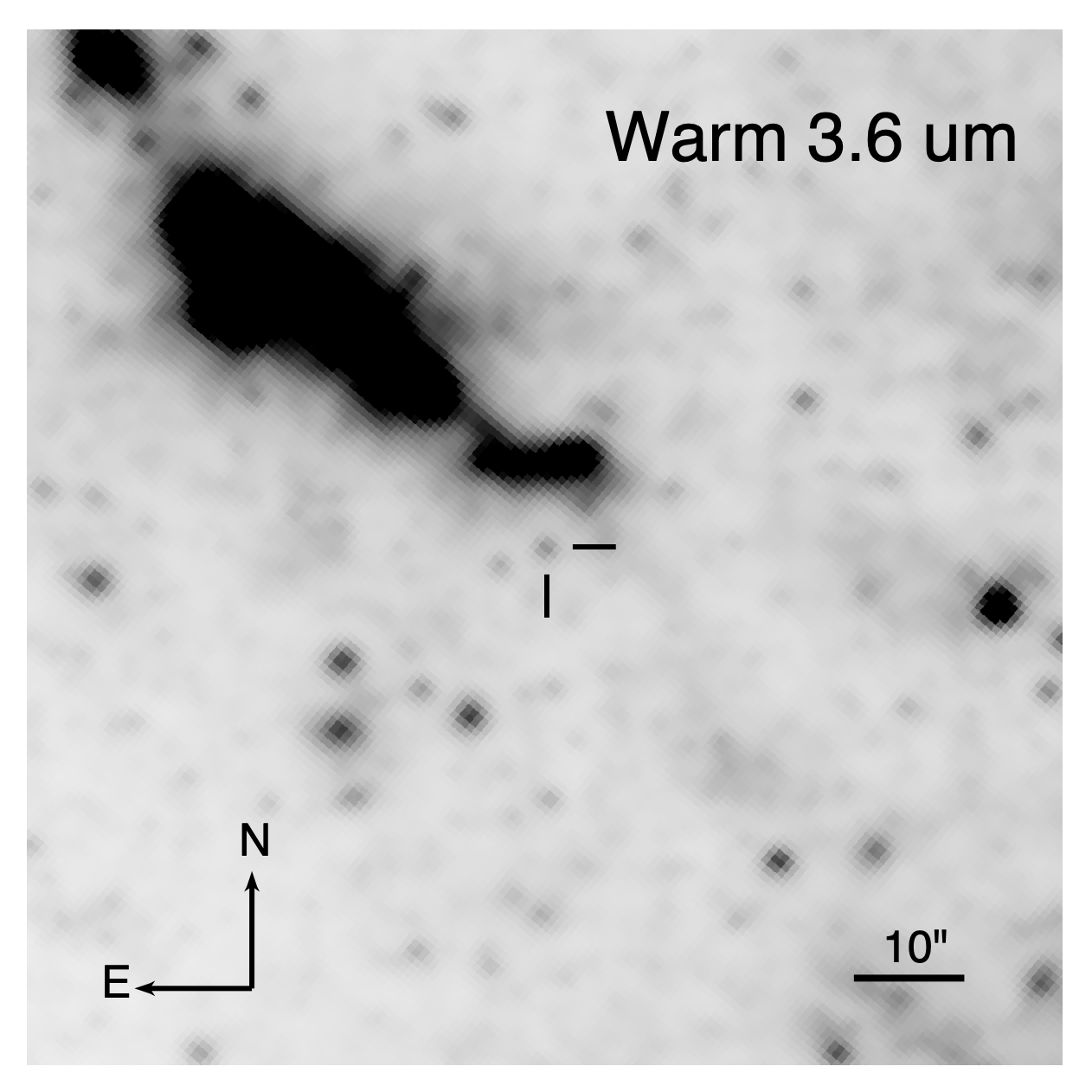
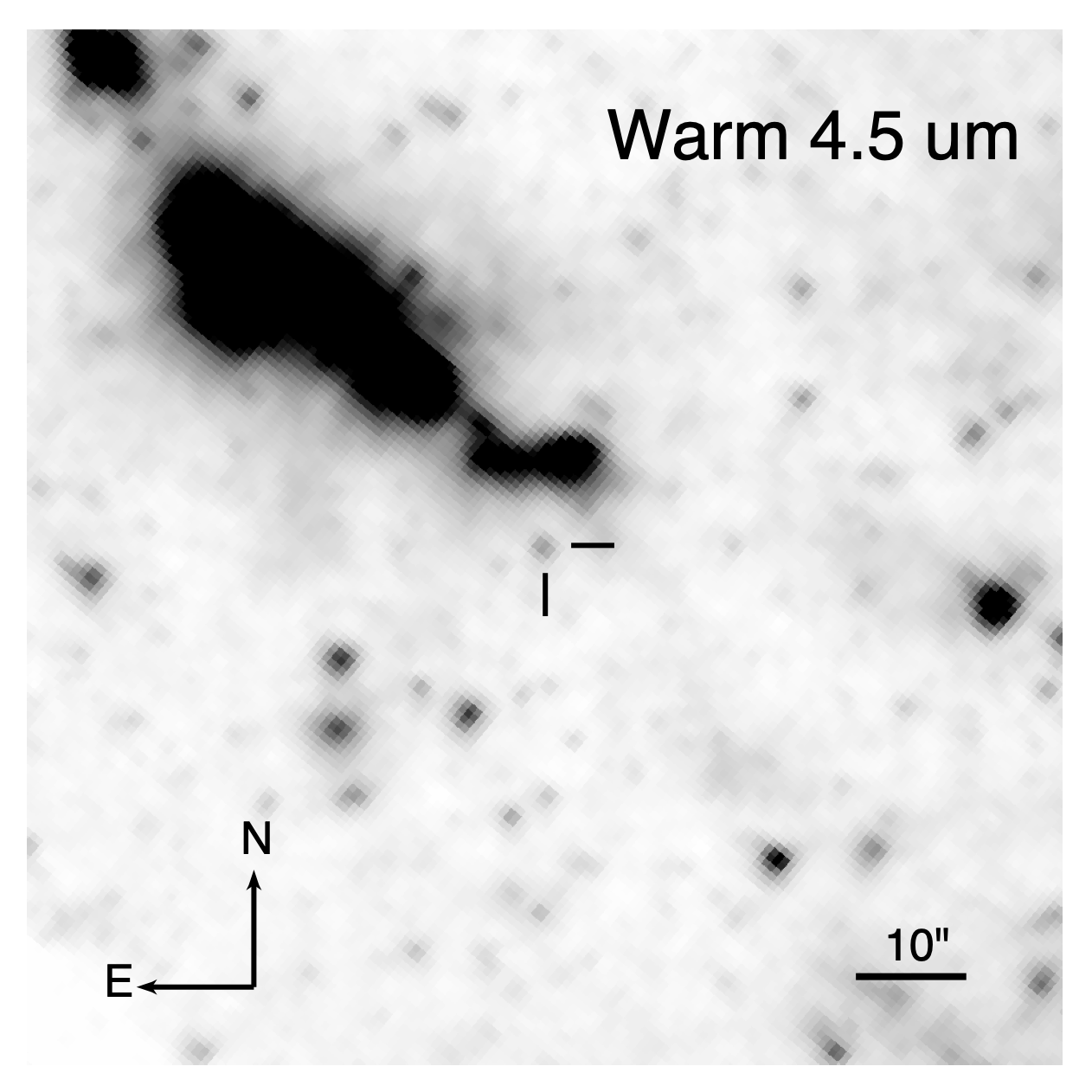
Figure 1: Pre-explosion Spitzer Warm Mission mosaics at Channels 1 and 2 (3.6 and 4.5 $\mu$m, respectively). A source can be clearly seen at the absolute position of SN 2023ixf in both channels, which we identify as its progenitor candidate in the mid-IR.

Since M101 was a target of several programs during the Spitzer mission, we checked the Spitzer Heritage Archive (SHA; at the NASA/IPAC Infrared Science Archive, or IRSA) for available data, in order to follow the photometric evolution of the progenitor on the archival mid-infrared (mid-IR) images. A single-epoch dataset exists during the Spitzer Cryogenic Mission (2004 March 08, PID 60 [GORDON-M101], PI: G. Rieke), while the field of the SN was imaged on many additional epochs between 2012 and 2019 (mostly during the SPIRITS program, Kasliwal et al. 2017; PIDs 10136, 11063, 13053, 14089; PI: M. Kasliwal). A point source is clearly detectable on 3.6 and 4.5 $\mu{\rm m}$ (Channels 1 and 2, respectively; see Fig. 1) Spitzer/IRAC images at the position of the SN at all epochs between 2004 and 2019, while there is no detection on 5.8 and 8.0 $\mu{\rm m}$ images obtained in 2004. We considered this source to be the progenitor candidate and reported on our preliminary analysis in Szalai & Van Dyk (2023), whereby we determined the mid-IR fluxes of the source by applying simple aperture photometry on the 3.6 and 4.5 $\mu$m Spitzer/IRAC post-basic calibrated (PBCD) images. The measurements showed some possible flux changes, though below the photometric uncertainties, in the preceding $19$ yr before the explosion. If this variability is real, it could be an indication of possible internal pulsational instabilities and pre-explosion mass-loss processes occurring in the star years prior to explosion. Hence, we carried out a more careful analysis of the archival Spitzer/IRAC data of the object, concurrent with that of Kilpatrick et al. (2023) and Jencson et al. (2023).

Rather than continuing with the PBCD mosaics, we obtained the artifact-corrected cBCD frames (along with the corresponding uncertainty and mask frames) for each epoch. The Cryogenic and Warm data were treated separately. We further selected for each epoch only the frames covering the location of the progenitor candidate. We then performed overlap correction and mosaicking of these frames with MOPEX (Makovoz & Khan, 2005). We invoked the task APEX User List Multiframe, with the absolute SN position as input, to extract the flux via fitting of the Point Response Function (PRF) for each epoch. A visual spot-check of the residual mosaics after the PRF fitting, generated with APEX QA, revealed a clean subtraction of the PRF model in each case. We list the Spitzer flux densities, along with their formal uncertainties (based on SNR), in Table 1. We note that the absolute photometric calibration of the entire Spitzer mission is better than 3% (Carey et al., 2012).

To validate our PRF photometry results and to provide more realistic estimates of the uncertainties, we injected an artificial star into the cBCD frame for each epoch, with a flux equal to that estimated for the progenitor candidate, at a distance of $8{\farcs}4$ east-southeast of the candidate, in an empty region with a qualitatively similar background as the candidate, using APEX QA. The overlap, mosaic, and PRF estimation steps were then repeated, with both the candidate and the artificial star extracted. We found for both bands that the flux of the artificial star was on average ca. $3\ \mu$Jy, or $11$%, brighter than the estimate for the candidate. A similar spot check of the residual mosaics, again, indicated clean and complete PRF fitting for both the candidate progenitor and the artificial star. We have therefore included this slight flux excess into the uncertainties for the measurements in each epoch.

To convert the flux densities into Vega magnitudes, we adopted the IRAC zeropoints, $272.2\pm 4.1$ Jy and $178.7\pm 2.6$ Jy at the nominal channel wavelengths of 3.544 and $4.487\ \mu$m, respectively. The light curves for these two channels are shown in the top panel of Fig. 2. Significant variability can be clearly seen. We measure a root-mean-square (RMS) amplitude of 0.23 and 0.26 mag for Channels 1 and 2, respectively, in good agreement with the average variation found by Reiter et al. (2015) for Galactic long-period variables (LPVs).

Kilpatrick et al. (2023) have also used this same Spitzer data set and noted the variability, which is similar to our value of 0.7 mag peak-to peak. Their measured fluxes are, however, $\sim 5\mbox{--}10~{}\mu{\rm Jy}$ lower than ours, which is likely due to differences in the photometry methods. They have performed sanity checks to ascertain that the variability is intrinsic to the star and not due to instrumental or spacecraft-related systematic effects. Hence, we proceed below considering the variability to be indeed intrinsic to the star. Additionally, in the archival HST ACS/WFC F814W pre-explosion image, there is possibly an indication of blending of the progenitor star candidate with another (fainter) source located $0{\farcs}1$ from it (e.g., Pledger & Shara, 2023; Kilpatrick et al., 2023). However, the observed mid-IR variability is likely dominated by a single source (see Sect. 3).

Jencson et al. (2023) also analyzed the archival Spitzer data of the assumed progenitor in detail. They identified the same source as we did, carried out PSF photometry on the Cryogenic Mission data and, following that, performed image subtraction and aperture photometry on the Warm Mission data using the Cryogenic mosaic images as templates. Results of their $4.5~{}\mu{\rm m}$ photometry agree well with ours; however, for the $3.6~{}\mu{\rm m}$ photometry, there is an offset similar to that of Kilpatrick et al. (2023). We note that the discrepancies likely arise from differences in the photometric techniques. The general light curve variability, however, is the same between this work and that of Jencson et al. (2023) and Kilpatrick et al. (2023). Thus, the offsets in the photometry noted above do not affect the main results of our paper, which are based on the variability in the light curves, in particular their period analysis (cf. Sect. 3). We find a similar period using the $3.6~{}\mu{\rm m}$ light curve from Jencson et al. (2023) as well as the one from Kilpatrick et al. (2023).

2.2 Gemini NIRI

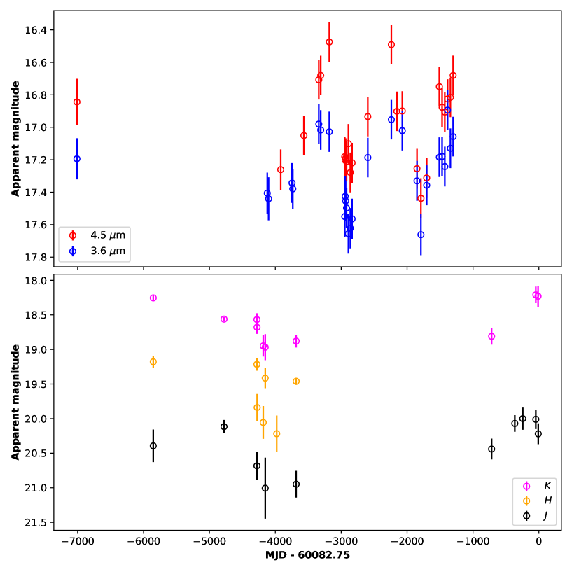
Figure 2: Light curves of the progenitor candidate in the mid-IR based on Spitzer data (upper panel) and the near-IR based on UKIRT/WFCAM and Gemini/NIRI data, along with MMT/MMIRS data reported by Jencson et al. (2023) (lower panel). The x-axis origin corresponds to the explosion epoch of SN 2023ixf (Hosseinzadeh et al., 2023).

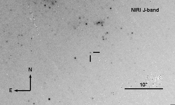
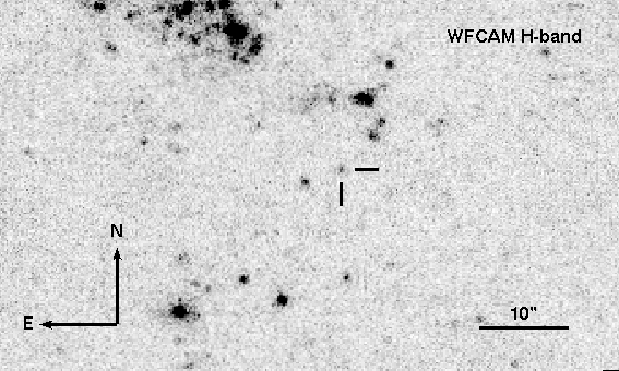
Figure 3: Cutouts around the progenitor candidate for SN 2023ixf from archival NIRI $K$-band (top left), $J$-band (top right), and UKIRT/WFCAM $H$-band (bottom) images.

We searched the Gemini Science Archive (Hirst & Cardenes, 2016) for any available pre-explosion data at the position of SN 2023ixf. There are observations taken with the Near-IR Imager (NIRI; Hodapp et al. 2003) on 2010 April 18 (UT) for the program GN-2010A-Q-27 (PI: G. Bosch) to study the HII region NGC 5461 located near to SN 2023ixf, thus providing serendipitous pre-explosion imaging for the latter. This program used two filters—$K$-continuum and narrow-band Br(gamma) with central wavelengths $2.0975~{}\mu{\rm m}$ and $2.1686~{}\mu{\rm m}$, respectively. There are 26 exposures of Br(gamma) and 51 exposures of $K$-continuum, each of 50 sec. In addition, there are two $J$-band acquisition images, each with an exposure time of 30 sec. In the following, we do not use the narrow-band data as the wavelength is already covered by the $K$-continuum band.

We reduce these data with Gemini’s DRAGONS software (Labrie et al., 2019) using its recipe for NIRI imaging data, which performs dark subtraction, masking of bad pixels, flat fielding, sky subtraction, image registration, and stacking. The image quality for one of the $J$-band acquisition images is rather poor, so we do not include that exposure. For this filter, we thus have only one image so no sky subtraction has been performed for it by the DRAGONS processing. This does not affect our result, since the background is subtracted during the downstream processing for photometry.

A point source at the position of SN 2023ixf is clearly detected in both the $K$-continuum and $J$-band images as shown in Fig. 3. We perform PSF photometry using the Photutils package of Python (Bradley et al., 2022) and apply the aperture correction resulting from a curve-of-growth analysis for each image. Since there are only two 2MASS stars in the NIRI image, we calibrate the final photometry using five isolated stars in the images by comparing their instrumental magnitudes to corresponding calibrated magnitudes measured from the UKIRT/WFCAM data discussed below (Sect. 2.3). We thus obtain $J=20.12\pm 0.10$ mag and $K=18.56\pm 0.03$ mag for the progenitor (cf. Table 2).

We note that Kilpatrick et al. 2023 have also used the $K$-continuum data from this Gemini program (but not the $J$-band data), and calibrated their result against the NOIRLab Extremely Wide Field Infrared Imager (NEWFIRM) $K$ data observed around the same time (2010 June–July). They measured a value of $K=20.72\pm 0.08$ AB mag from the NIRI data for the progenitor candidate, which is $18.87\pm 0.08$ converted to Vega mag; they obtained a similar value for the NEWFIRM $K$ data. Their result is about 0.3 mag fainter than ours. This could perhaps be due to differences in the data processing. Since the NEWFIRM data do not add any additional information to that already contained in the Gemini data, we do not consider it further in our analysis.

2.3 UKIRT/WFCAM

We also searched the archival data gathered by the near-infrared (near-IR) Wide Field Camera (WFCAM; Casali et al. 2007) on the 3.8 m United Kingdom Infrared Telescope (UKIRT). Science-quality reduction of the WFCAM data is performed by the automated WFCAM/VISTA pipeline at the Cambridge Astronomical Survey Unit (Irwin et al., 2004) and the data products are then ingested into the WFCAM Science Archive (WSA; Hambly et al. 2008). Astrometric and photometric calibrations, both tied to 2MASS (Skrutskie et al., 2006), are carried out as part of the pipeline processing. In particular, the pipeline derives a final photometric calibration in the WFCAM system (see Hodgkin et al. 2009 for details).

We find 41 images for each of $J$-, $H$-, and $K$-band between 2007 and 2013, with exposure times ranging from 1 to 20 sec. The project IDs for these observations are U/11B/K1, U/11B/K2, U/11B/K4, U/12A/KASI1, U/13A/K1, and U/SERV/1745. Since many of the images are shallow and taken close in time, we decide to stack all the images observed in the same month in a given year. The stacking is not expected to affect our analysis since the timescale of variability for RSGs is typically $100$ d or greater (e.g., Jurcevic et al., 2000; Kiss et al., 2006; Yang & Jiang, 2011, 2012; Wasatonic et al., 2015; Soraisam et al., 2018; Ren et al., 2019; Chatys et al., 2019). A source can be clearly seen at the position of SN 2023ixf in many of the images (e.g., the $H$-band image taken on 2007 May 10 (UT), shown in Fig. 3, bottom panel), which we consider as the progenitor candidate in the near-IR.

We perform (forced) PSF photometry on the WFCAM data at the SN position obtained from its first detection at $g=15.90\pm 0.03$ on 2023 May 19 (UT) by the ZTF survey (Bellm et al., 2019). It is to be noted that the astrometric accuracy for ZTF (tied to Gaia DR1) is better than a few tens of milliarcsec for bright sources (see Masci et al. 2019), while that for WFCAM is $0{\farcs}1$ (Hodgkin et al., 2009). For all three filters, the offset between the PSF-fitted position of the progenitor candidate and that of the SN is less than 1 pixel (i.e., $0{\farcs}2$) of the WFCAM image. Similar to that of NIRI data, we then determine the aperture correction for the PSF photometry from a curve-of-growth analysis. The total instrumental magnitude is then calibrated using the available zero-point of the image. The resulting near-IR measurements are given in Table 2 and the light curves are shown in Fig. 2.

We also plot the most recent $J$ and $K$ photometry of the progenitor candidate obtained by Jencson et al. (2023) using MMT/MMIRS. These are the data points within 1000 d of the explosion in Fig. 2, lower panel. From the sparse near-IR light curves, we obtain RMS amplitudes of 0.36, 0.38, and 0.28 mag, respectively, for the $J$-, $H$-, and $K$-band.

3 Analysis

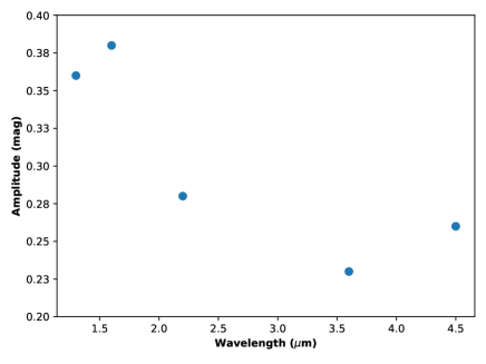
Figure 4: Variation of light curve RMS-amplitude of the progenitor candidate as a function of wavelength.

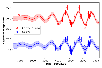
Figure 5: Left: Reconstructed power spectrum of the Spitzer $3.6~{}\mu{\rm m}$ light curve with its 99 percent confidence interval highlighted by the gray shaded region. The gray dotted line marks the location of the identified period. Right: Reconstructed light curves using the power spectrum on the left for the Spitzer 3.6 and $4.5~{}\mu{\rm m}$ data shown by the blue and red curves, respectively. The shaded color regions mark their $1\sigma$ confidence intervals.

In Fig. 4, we show the RMS amplitudes from the mid-IR and near-IR light curves as a function of wavelength. There is a clear indication of an increase in variability amplitude with decreasing wavelength, which is in line with expectations for RSGs and other LPVs. For example, Wasatonic et al. (2015) analyzed 17 yr of $V$-band and narrow- to intermediate-band near-IR high-cadence time-series photometry of the Galactic RSG TV Gem and found the peak-to-peak amplitude to increase from 0.3 mag in the near-IR to over $1$ mag in the $V$-band. Similarly, Wood et al. (1983) measured a $K$-band amplitude of $\lesssim 0.25$ mag for RSGs in the Large and Small Magellanic Clouds, while Yang et al. (2018) found an amplitude $\lesssim 0.3$ mag in the mid-IR (WISE1- and WISE2-band) for the sample of RSGs in the Large Magellanic Cloud that they studied. Also, Boyer et al. (2015) cross-identified variable sources from the DUSTiNGS survey with LPVs that have been observed in the optical and near-IR and found the variability amplitude to increase with decreasing wavelength.

We perform a period analysis using the Spitzer light curves. As described in previous work by various authors, e.g., Kiss et al. (2006), Soraisam et al. (2018), light curves of RSGs present complex morphologies, characterized by the superposition of a strong red-noise component and one or multiple distinct frequencies. For analysis of such semi-regular variables, conventional methods like Lomb-Scargle periodogram may be inadequate (VanderPlas, 2018). We therefore utilize the same Bayesian model used by Soraisam et al. (2018) for the period analysis of optical light curves of RSGs in M31. Specifically, we describe the $3.6~{}\mu{\rm m}$ light curve as a Gaussian Process using the NIFTy software package (Selig et al., 2013; Steininger et al., 2019; Arras et al., 2019). With the latter we simultaneously reconstruct the underlying signal and its unknown power spectrum from the observed light curve data and reported uncertainties (see Sect. 2.4 of Soraisam et al. 2018 for details), by sampling an approximate representation of the joint posterior distribution of light curve and power spectrum. The results are shown in Fig. 5.

We use the recovered power spectrum from the $3.6~{}\mu{\rm m}$ data to model the $4.5~{}\mu{\rm m}$ light curve, again as a Gaussian Process but this time with a fixed power spectrum, which is highlighted in the right panel of Fig. 5. As can be clearly seen, the reconstructed light curve fits the data well, which implies that the periodicity seen in both the Spitzer channels is the same, likely due to both of them having the same physical origin. We obtain similar results when executing this process in reverse, i.e., using the $4.5~{}\mu{\rm m}$ data for inferring the power spectrum and using it to model the $3.6~{}\mu{\rm m}$ light curve.

For each of the posterior power spectrum samples, we determine the frequency corresponding to the power maximum (peak frequency). We then use the median of these peak frequencies to define the period for the Spitzer $3.6~{}\mu{\rm m}$ light curve, obtaining $1091\pm 71$ d (marked by the dotted line in Fig. 5, left panel), where the uncertainty is derived from the width of the distribution of peak frequency values.

As mentioned in Sect. 2.1, there is possibly a fainter source located close to the progenitor candidate in the optical HST F814W pre-explosion image. This opens up the question of possible blending of sources (including those not visible in the optical) for the mid-IR data, given their poorer spatial resolution as compared to HST. We argue that it is unlikely that all the blended sources vary with exactly the same dominant frequency to give rise to the peak in the power spectrum in Fig. 5. The observed variability at the position of SN 2023ixf therefore most likely results from a single source, and we attribute that to the RSG progenitor candidate.

4 Discussion

4.1 Pulsational instabilities?

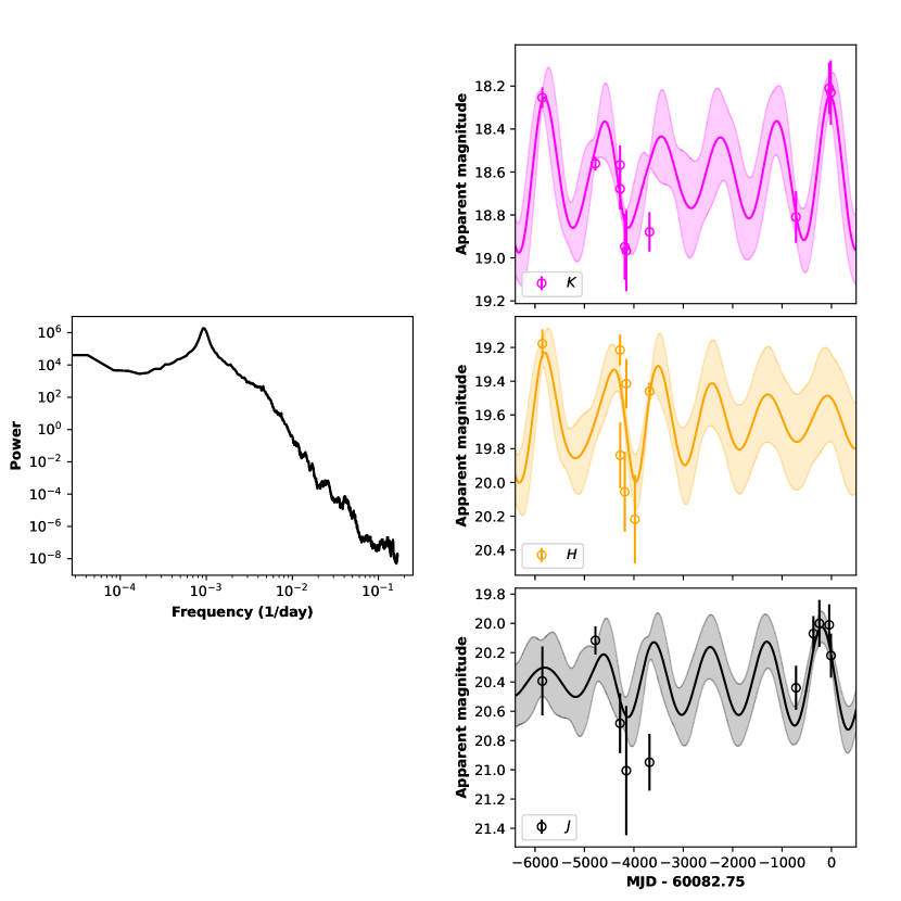
Figure 6: Near-IR light curve models for the progenitor candidate of SN 2023ixf constructed using the power spectrum on the left, which is recovered from the Spitzer data (Fig. 5 left) scaled by a factor 2.2 to account for the larger variability amplitude in the near-IR (Fig. 4). The shaded regions indicate the $1\sigma$ confidence intervals for the models. Despite the scarce data points, the light curves look reasonable as compared to those built using various modified versions of the power spectrum shown in Figs. 8, 9, 10.

The near-IR emission of RSGs is dominated by light from the stellar photosphere. To ascertain whether the same periodicity can also explain the near-IR light curves, we model the latter using the power spectrum of the Spitzer $3.6~{}\mu{\rm m}$ light curve obtained above. Given the slightly larger amplitude of the near-IR light curves as compared to the mid-IR (Fig. 4), we scale this power spectrum by a factor 2.2, which is the average of the ratios of the squares of the amplitudes in the near-IR to the mid-IR. The resulting models are shown in the right panel of Fig. 6. As is evident from the plots, the models agree well with the data, implying the presence of the same periodicity in the near-IR data and, in turn, indicating again a common driver for the variability observed in both the near-IR and mid-IR regimes. We further demonstrate in Appendix A that similar frequencies are needed to explain the near-IR data, by showing reconstructions performed with power spectra where the peak around a period of 1091 d is absent.

Indeed, near-IR variability in RSGs driven by pulsation has been established for decades (e.g., Wood et al., 1983). As discussed in Sect. 3, the near-IR amplitudes for the progenitor candidate are also in agreement with those of other known pulsating RSGs and therefore we conclude that pulsational instabilities in the progenitor star are likely responsible for its observed variability.

As shown by Davies et al. (2022, see their Fig. 3), mid-IR emission from the pre-SN outburst models stays almost constant, while the optical and near-IR bands may be significantly affected and thereby provide the best diagnostic for such outbursts. The MMT/MMIRS $J$ and $K$ band observations taken less than two weeks prior to the SN explosion appear to follow the general variability trend in the near-IR going back $16$ yr based on the WFCAM and NIRI data (Fig. 6), thus supporting the results obtained by other groups that there was likely no pre-SN outburst (Kilpatrick et al., 2023; Neustadt et al., 2023; Jencson et al., 2023; Dong et al., 2023). There are not enough deep optical observations of the progenitor prior to explosion to measure the variability that is typically present for RSGs in this wavelength regime. However, assuming its pulsational instability to be similar to that in common RSGs, it is likely to have a larger variability amplitude in the optical. For the RSG TV Gem, Wasatonic et al. (2015) measured the $V$-band amplitude to be a factor $4$ larger than that in the near-IR. Using the same scaling, we estimate the optical amplitude of the RSG progenitor candidate to be around 1.6 mag.

4.2 Estimates of the progenitor’s initial mass and mass-loss rate

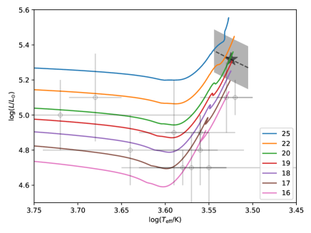
Figure 7: HR diagram based on the BPASS single star evolutionary tracks. Different colors indicate different initial masses of the models as indicated in the legend (in ${\rm M}_{\odot}$). The gray shaded parallelogram around the $\bigstar$-symbol shows the possible location of the progenitor candidate of SN 2023ixf, assuming a late M-type supergiant with $T_{\rm eff}$ ranging from $3200\mbox{--}3500$ K (see text). The vertical width of the region corresponds to the uncertainty in $\log(L/L_{\odot})$ at a given temperature. The faint gray crosses mark the locations of cool and luminous ($\log(L/L_{\odot})>4.7$), directly detected progenitors of previous SNe-IIP/II-L from Smartt (2015) and Van Dyk (2017).

We use the period of 1091 d derived above (Sect. 3) and the period-$M_{K}$ (PL) relation for RSGs from Soraisam et al. (2018) to compute the absolute magnitude of the progenitor candidate in $K$-band. This method, which is fundamentally different from the widely used SED fitting, provides an estimate of the luminosity of the star that does not rely on using extinction information or the distance to the host galaxy. We thus obtain a value of $M_{K}=-11.58\pm 0.31$ mag. Soraisam et al. (2018) noted a dispersion of 0.29 mag around their period-$M_{K}$ relation. We have included this as well as the uncertainty in our derived period in the calculation of the final uncertainty of our $M_{K}$ estimate here. We note that we obtain values of $M_{K}$ that agree with our estimate within the uncertainties when using other published PL relations for RSGs (e.g., Kiss et al., 2006; Yang & Jiang, 2012). This may be expected since the PL relation for RSGs appears to be universal (cf. Fig. 7 of Soraisam et al. 2018).

Jencson et al. (2023) report a foreground-extinction-corrected and phase-weighted mean absolute magnitude of $M_{K}=-10.7$ mag directly computed from the observed light curve. This value is not corrected for CSM extinction, which is likely to be significant for the progenitor candidate. In addition, it will be sensitive to uncertainties in distance and interstellar extinction estimates. Nevertheless, it can be considered as a lower limit for the actual $M_{K}$, and thus, our brighter $M_{K}$ value is consistent with their result.

Taking into account this high value of $K$-band absolute brightness, as well as its near- and mid-IR colors ($[3.6]-[4.5]\approx 0.3$ mag, $J-K\approx 1.8$ mag), the assumed progenitor of SN 2023ixf seems to be among the most luminous RSG stars (for comparison, see the results of large-scale AGB/RSG surveys in nearby galaxies by Boyer et al. 2015; O’Grady et al. 2020; Massey et al. 2023). In the SPIRITS sample analyzed by Bond et al. (2022), there are some objects (e.g., 15ahg, 15wt) with mid-IR light-curve periods and amplitudes, absolute magnitudes, and colors similar to that of the progenitor of SN 2023ixf; these objects are found to be mostly similar to dusty OH/IR stars by the authors. Such objects are known to undergo intensive mass-loss during the so-called superwind phase (Iben & Renzini, 1983). Jencson et al. (2023) have shown via comparison of the progenitor candidate’s SED with superwind-based models from Davies et al. (2022) that it likely underwent such a phase of enhanced mass-loss (rather than an outburst) over the final decades of its life.

In Paper II, we perform SED-fitting of the progenitor candidate using the Grid of Red supergiant and Asymptotic giant branch star ModelS (GRAMS; Sargent et al. 2011; Srinivasan et al. 2011). In addition to uncertainties in distance and interstellar extinction toward the star, SED fitting is also sensitive to limitations in the models used, for example, coarse sampling of $T_{\rm eff}$ and optical depth parameters in the available GRAMS grid. We circumvented the latter issue in Paper II by training an emulator (see Paper II for details). However, we find that the $T_{\rm eff}$ value is not well constrained—the fit allows a large range from around 2400 K to 3700 K. Such a large range is consistent with the inferred relatively high dust obscuration of the progenitor candidate, which makes it difficult to predict the stellar parameters, in particular given that the sparse data in the mid-IR (covering only $3.6~{}\mu{\rm m}$ and $4.5~{}\mu{\rm m}$) only poorly constrain the dust content.

As noted above, the mid-IR properties of the progenitor candidate appear to be consistent with those of dusty OH/IR stars. Such stars typically have a late M spectral type—for example, M7 for IRC -10414 (cf. Gvaramadze et al. 2014), M6 for NML Cyg, M4–M9.5 for VX Sgr, M3–M4 for S Per (Schuster et al., 2006), and M5 for WOH G64 (Levesque et al., 2009). Thus, to be completely independent of the SED-fitting results, we adopt the $T_{\rm eff}$ range of $3200\mbox{--}3500$ K spanned by M4 and later spectral type RSGs. We use the corresponding bolometric correction to the $K$-band ($BC_{K}$) determined by Levesque et al. (2005) based on the MARCS stellar atmosphere models for cool stars to convert the absolute $K$-band magnitude to bolometric luminosity. The values of $BC_{K}$ range from 3.16 to 2.92 mag, decreasing with increasing temperature.

We thus obtain an absolute bolometric magnitude $M_{\rm bol}=-8.42\pm 0.31$ mag and a corresponding $\log(L/L_{\odot})=5.27\pm 0.12$ at the lowest $T_{\rm eff}=3200$ K considered above, and $M_{\rm bol}=-8.66\pm 0.31$ mag and corresponding $\log(L/L_{\odot})=5.37\pm 0.12$ at $T_{\rm eff}=3500$ K. We note that the luminosity derived here from the PL relation is about $0.2\mbox{--}0.3$ dex higher than that obtained from SED fitting (Paper II, Jencson et al. 2023).

The typical mass-loss rate for RSGs is in the range $10^{-7}\mbox{--}10^{-4}~{}{\rm M}_{\odot}~{}{\rm yr}^{-1}$ (e.g., Mauron & Josselin, 2011), while that for OH/IR stars is in the range $10^{-5}\mbox{--}10^{-3}~{}{\rm M}_{\odot}~{}{\rm yr}^{-1}$ (e.g., Justtanont et al., 2013). Goldman et al. (2017) derived an empirical mass-loss prescription for AGBs/RSGs in the superwind phase. They found that the mass-loss rate mainly correlates with the pulsation period and luminosity. We use their relation $\dot{M}=4.2\times 10^{-11}L^{0.9}P^{0.75}r_{\rm gd}^{-0.03}$, where $\dot{M}$ is the mass-loss rate (in ${\rm M}_{\odot}~{}{\rm yr}^{-1}$), $L$, the luminosity (in $L_{\odot}$), $P$, the period (in days), and $r_{\rm gd}$, the gas-to-dust ratio, to estimate the progenitor candidate’s mass-loss rate assuming it to be in the superwind phase as described above. These authors showed that the prescription does not strongly depend on the gas-to-dust ratio, so we assume a typical value of 200. Then, using the period and luminosity of the progenitor candidate, we obtain its mass-loss rate to be $(2\mbox{--}4)\times 10^{-4}~{}{\rm M}_{\odot}~{}{\rm yr}^{-1}$, which is also within the range obtained from SED modeling by Jencson et al. (2023), but lower than the estimate in Paper II. The latter can be reconciled by adopting a higher value for the wind velocity (e.g., $\sim 50$ km/s) appropriate for the superwind phase in the GRAMS SED modeling. The higher velocity does not change the $T_{\rm eff}$ result in Paper II. Our mass-loss rate estimate here is also in agreement with that obtained by Grefenstette et al. (2023) based on early hard X-ray observations of SN 2023ixf.

We estimate the initial mass of the progenitor candidate using the Binary Population and Spectral Synthesis (BPASS; Stanway & Eldridge 2018) single-star evolutionary tracks. The metallicity of the host galaxy M101 at the site of the SN explosion is likely solar (see Paper II). We therefore use the BPASS stellar models for solar metallicity. Using the $T_{\rm eff}$ range and corresponding luminosity derived above for the RSG progenitor candidate, we plot the latter on the Hertzsprung-Russell (HR) diagram shown in Fig. 7.

We estimate the zero-age main sequence (ZAMS) mass of the progenitor candidate by comparing its luminosity to the terminal points of the tracks. We thus obtain its ZAMS mass of $20\pm 4~{}{\rm M}_{\odot}$. Within the uncertainty, this agrees with the higher end of the mass range obtained from SED fitting with the GRAMS dust models ($17\pm 4~{}{\rm M}_{\odot}$ by Jencson et al. 2023; see also Paper II). It, however, rules out the lower values $11\mbox{--}12~{}{\rm M}_{\odot}$ obtained by Kilpatrick et al. (2023) and Pledger & Shara (2023). Our ZAMS mass estimate, therefore, also constrains the different initial-mass results between Jencson et al. (2023), Paper II, and Kilpatrick et al. (2023), which are all based on SED fitting, by using an independent method (i.e., the PL relation).

Based on our result above, the progenitor candidate of SN 2023ixf appears to be among the most massive progenitors detected so far for core-collapse SNe. Its inferred ZAMS mass of $20\pm 4~{}{\rm M}_{\odot}$ puts into question the existence of the red supergiant problem (Smartt, 2015), i.e., the apparent high-mass cut-off at around $18~{}{\rm M}_{\odot}$ for RSG stars exploding as SNe despite their high-mass limit of $25\mbox{--}30~{}{\rm M}_{\odot}$ predicted by stellar evolution theory. To-date, a few dozen core-collape SN progenitors have been directly identified (see Van Dyk 2017 for a review). Among them, there already exist progenitors with masses close to this limit, for example, SN 2013 ej (Van Dyk, 2017). Furthermore, various other studies, e.g., Davies & Beasor (2018, 2020), have shown that the problem of missing high-mass progenitors of SNe II-P/L is not statistically significant and could be explained by the small sample size of the SN progenitors and a steep luminosity function for the RSGs. Our result thus supports this hypothesis.

4.3 Binary system?

Other possible origins of variability in luminous near- and mid-IR stellar sources, as described in detail by Karambelkar et al. (2019), are the presence of interacting dusty winds in massive (Wolf-Rayet) binary stars and/or orbital modulation of the binary systems. As presented in that work and references therein, such dusty binary systems could be heavily obscured in the optical, giving a possible explanation for the non-detection of the assumed progenitor system of SN 2023ixf with HST F435W and F555W filters (see, e.g., Soraisam et al. 2023; Kilpatrick et al. 2023, Paper II). Both the observed IR light-curve amplitudes and period could be explained with the orbital modulation of a massive dusty binary. However, based on the results presented above (IR colors, similarity to identified pulsators), a long-period RSG star seems to be the primary candidate for the progenitor of SN 2023ixf.

On the other hand, we note that Kilpatrick et al. (2023) also carried out a binary population synthesis analysis using the HST flux upper limits and found that a close binary as a progenitor system for SN 2023ixf cannot be ruled out. However, although the binary fraction of massive OB-type stars is regarded to be more than 70% (e.g., Sana et al., 2012), recent studies have found a fraction of $20\%$ or less for RSGs with OB-type companions (Neugent et al., 2020), making this model rather unlikely. As Kilpatrick et al. (2023) have also noted, the presence of a possible companion star could only be revealed with deep optical imaging after the SN fades.

5 Conclusions

The proximity of SN 2023ixf, along with its host galaxy M101 being a frequent target for various imaging campaigns in different wavelengths, have facilitated detection and detailed studies of its progenitor candidate. Here we used archival mid- ($3.6~{}\mu{\rm m}$ and $4.5~{}\mu{\rm m}$) and near-IR $JHK$ data from the Spitzer Space Telescope and ground-based facilities (Gemini North, UKIRT, MMT) to characterize the variability of the progenitor candidate, covering a combined duration of around 19 yr prior to the SN explosion. We find its RMS amplitudes in these wavelengths to be in the range of $0.2\mbox{--}0.4$ mag, increasing with decreasing wavelength. From a rigorous period analysis of the higher-cadence Spitzer $3.6~{}\mu{\rm m}$ and $4.5~{}\mu{\rm m}$ data, we determine a period of $1091\pm 71$ d. We demonstrate that the same periodicity is also present in the $JHK$ light curves, thus indicating a common physical origin for the observed variability in both mid- and near-IR. The variability characteristics taken together with the infrared colors are consistent with those of pulsating RSGs.

Using the period-luminosity relation for RSGs from Soraisam et al. (2018), we compute an absolute $K$-band magnitude of $-11.58\pm 0.31$ mag. We then use the range of $T_{\rm eff}$ covered by late M-type RSGs and their corresponding bolometric corrections to derive the luminosity, $\log(L/L_{\odot})$, for the progenitor candidate. We obtain a range of $5.27\pm 0.12$ dex at $T_{\rm eff}=3200$ K, the lowest value considered, to $5.37\pm 0.12$ dex at $T_{\rm eff}=3500$ K, the highest value considered. This thus gives an estimate of the luminosity independent of SED fitting for the RSG progenitor candidate. Assuming the latter to be in the superwind phase (with enhanced dust-driven mass-loss) over the final decades before the explosion (see, e.g., Jencson et al., 2023) and using its luminosity, pulsation period, and the mass-loss prescription of Goldman et al. (2017), we estimate its mass-loss rate. We find a value of $(2\mbox{--}4)\times 10^{-4}~{}{\rm M}_{\odot}~{}{\rm yr}^{-1}$, in agreement with the results from other authors (e.g., Grefenstette et al., 2023; Jencson et al., 2023). Finally, comparing the above luminosity with stellar models, we obtain a zero-age main sequence mass of $20\pm 4~{}M_{\odot}$ for the progenitor candidate of SN 2023ixf, which places it among the most massive progenitors detected so far for type II SNe.

Table 1: Spitzer IRAC Flux Densities

		3.6 $\mu$m		4.5 $\mu$m
AORKEY	MJD	Flux Density	Unc.	Flux Density	Unc.
		($\mu$Jy)	($\mu$Jy)	($\mu$Jy)	($\mu$Jy)
4370432	53072.09	36.08	4.16	32.70	4.25
44605952	55960.72	29.68	3.43	$\cdots$	$\cdots$
44605696	55980.99	28.75	3.48	$\cdots$	$\cdots$
45237760	56165.01	$\cdots$	$\cdots$	22.27	2.52
48186624	56337.07	31.45	3.51	$\cdots$	$\cdots$
45237504	56348.11	30.41	3.39	$\cdots$	$\cdots$
48187392	56516.35	$\cdots$	$\cdots$	27.03	3.00
50627840	56742.84	43.93	4.89	37.08	4.11
50627328	56771.83	42.49	4.71	38.01	4.21
50627072	56902.01	42.06	4.75	45.96	5.08
52776448	57136.69	26.00	2.94	23.97	2.68
52776704	57144.06	29.15	3.27	23.49	2.63
52776960	57150.17	28.40	3.20	23.75	2.66
52777216	57163.71	27.29	3.08	23.31	2.59
52777472	57191.82	23.58	2.64	25.80	2.85
52777728	57220.79	24.33	2.75	21.91	2.44
52777984	57247.82	25.65	2.90	23.14	2.60
52778240	57486.85	36.33	4.03	30.10	3.35
60830720	57843.93	45.05	5.00	45.28	5.01
60830976	57926.90	$\cdots$	$\cdots$	31.01	3.44
60831232	58009.67	42.32	4.70	31.07	3.44
60831488	58232.95	31.83	3.56	22.39	2.50
60831744	58292.87	23.45	2.69	18.92	2.14
60832000	58380.22	31.04	3.47	21.24	2.37
66022400	58572.08	36.41	4.04	35.67	3.96
66022656	58614.39	36.55	4.07	31.72	3.51
66022912	58655.68	34.52	3.85	30.88	3.43
66023168	58697.50	47.56	5.27	33.25	3.69
66023424	58740.01	38.29	4.26	33.56	3.73
66023680	58781.31	40.92	4.55	38.02	4.21

Table 2: NIR Photometry

	$J$		$H$		$K$
MJD	Mag	Mag_err	Mag	Mag_err	Mag	Mag_err	Instrument
54230.	20.39	0.24	19.18	0.09	18.25	0.05	WFCAM
55304.	20.12	0.10	$\cdots$	$\cdots$	18.56	0.03	NIRI
55803.	20.68	0.20	19.22	0.09	18.57	0.09	WFCAM
55805.	$\cdots$	$\cdots$	$\cdots$	$\cdots$	18.68	0.10	WFCAM
55807.	$\cdots$	$\cdots$	19.84	0.19	$\cdots$	$\cdots$	WFCAM
55899.	$\cdots$	$\cdots$	20.06	0.24	18.95	0.15	WFCAM
55929.	21.01	0.44	19.41	0.15	18.97	0.19	WFCAM
56104.	$\cdots$	$\cdots$	20.22	0.26	$\cdots$	$\cdots$	WFCAM
56399.	20.95	0.19	19.46	0.05	18.88	0.09	WFCAM

Appendix A Reconstructed near-IR light curves with modified power spectra

Here we model the near-IR data of the progenitor candidate using modified versions of the power spectrum recovered from the Spitzer $3.6~{}\mu{\rm m}$ data (Fig. 5, Sect. 3). The main purpose is to investigate whether we obtain a good reconstruction of the observed data for different shapes of the power spectrum, in particular without the prominent power peak seen in the original spectrum.

We consider three flavors – (i) the same spectrum from Fig. 6 but interpolating across the power peak to remove it (Fig. 8), (ii) a power law fit to the original spectrum (Fig. 9), and (iii) a power peak superposed on this power law fit at some higher frequency that is not a harmonic of the original peak frequency (Fig. 10). As can be seen, in all three cases we obtain a poorer reconstruction of the near-IR light curves than with the original power spectrum (Fig. 6), thus demonstrating that modeling the near-IR data indeed requires excess power at the same frequencies as inferred for the mid-IR.

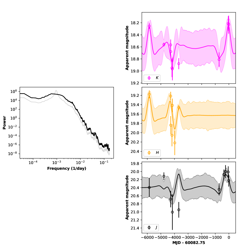
Figure 8: Modified form of the power spectrum recovered from the Spitzer data (left, cf. Sect. 3) and the near-IR light curve models for the progenitor candidate of SN 2023ixf constructed using it (right). The grey curve in the left panel shows the original power spectrum, while the shaded regions in the right panel indicate the $1\sigma$ confidence intervals for the light curve models. Here the modified power spectrum is obtained by interpolating across the power peak and scaling it to conserve the total power.

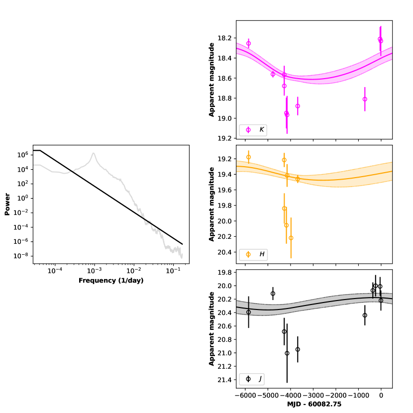
Figure 9: Similar to Fig. 8. Here the modified power spectrum is obtained by fitting a power law to the original spectrum from the Spitzer data and scaling it to conserve the total power. The flattening at the lowest frequency is due to extrapolation using the nearest neighbor value.

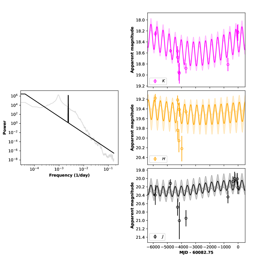
Figure 10: Similar to Fig. 8. Here the modified power spectrum is obtained by fitting a power law to the original spectrum from the Spitzer data, adding a peak at some higher frequency (which is not a harmonic of the original peak frequency) and scaling the resulting spectrum to conserve the total power. The flattening at the lowest frequency is due to extrapolation using the nearest neighbor value.

References

- Arras et al. (2019) Arras, P., Baltac, M., Ensslin, T. A., et al. 2019, NIFTy5: Numerical Information Field Theory v5, Astrophysics Source Code Library, record ascl:1903.008. http://ascl.net/1903.008
- Astropy Collaboration et al. (2013) Astropy Collaboration, Robitaille, T. P., Tollerud, E. J., et al. 2013, A&A, 558, A33, doi: 10.1051/0004-6361/201322068
- Bellm et al. (2019) Bellm, E. C., Kulkarni, S. R., Graham, M. J., et al. 2019, PASP, 131, 018002, doi: 10.1088/1538-3873/aaecbe
- Berger et al. (2023) Berger, E., Keating, G., Alexander, K., et al. 2023, Transient Name Server AstroNote, 131, 1
- Bond et al. (2022) Bond, H. E., Jencson, J. E., Whitelock, P. A., et al. 2022, ApJ, 928, 158, doi: 10.3847/1538-4357/ac5832
- Boyer et al. (2015) Boyer, M. L., McQuinn, K. B. W., Barmby, P., et al. 2015, ApJ, 800, 51, doi: 10.1088/0004-637X/800/1/51
- Bradley et al. (2022) Bradley, L., Sipőcz, B., Robitaille, T., et al. 2022, astropy/photutils: 1.5.0, 1.5.0, Zenodo, doi: 10.5281/zenodo.6825092
- Carey et al. (2012) Carey, S., Ingalls, J., Hora, J., et al. 2012, in Society of Photo-Optical Instrumentation Engineers (SPIE) Conference Series, Vol. 8442, Space Telescopes and Instrumentation 2012: Optical, Infrared, and Millimeter Wave, ed. M. C. Clampin, G. G. Fazio, H. A. MacEwen, & J. Oschmann, Jacobus M., 84421Z, doi: 10.1117/12.927183
- Casali et al. (2007) Casali, M., Adamson, A., Alves de Oliveira, C., et al. 2007, A&A, 467, 777, doi: 10.1051/0004-6361:20066514
- Chandra et al. (2023) Chandra, P., Maeda, K., Chevalier, R. A., Nayana, A. J., & Ray, A. 2023, The Astronomer’s Telegram, 16073, 1
- Chatys et al. (2019) Chatys, F. W., Bedding, T. R., Murphy, S. J., et al. 2019, MNRAS, 487, 4832, doi: 10.1093/mnras/stz1584
- Davies & Beasor (2018) Davies, B., & Beasor, E. R. 2018, MNRAS, 474, 2116, doi: 10.1093/mnras/stx2734
- Davies & Beasor (2020) —. 2020, MNRAS, 493, 468, doi: 10.1093/mnras/staa174
- Davies et al. (2022) Davies, B., Plez, B., & Petrault, M. 2022, MNRAS, 517, 1483, doi: 10.1093/mnras/stac2427
- Dong et al. (2023) Dong, Y., Sand, D. J., Valenti, S., et al. 2023, arXiv e-prints, arXiv:2307.02539, doi: 10.48550/arXiv.2307.02539
- Goldman et al. (2017) Goldman, S. R., van Loon, J. T., Zijlstra, A. A., et al. 2017, MNRAS, 465, 403, doi: 10.1093/mnras/stw2708
- Grefenstette et al. (2023) Grefenstette, B. W., Brightman, M., Earnshaw, H. P., Harrison, F. A., & Margutti, R. 2023, arXiv e-prints, arXiv:2306.04827, doi: 10.48550/arXiv.2306.04827
- Guo & Li (2002) Guo, J. H., & Li, Y. 2002, ApJ, 565, 559, doi: 10.1086/324295
- Gvaramadze et al. (2014) Gvaramadze, V. V., Menten, K. M., Kniazev, A. Y., et al. 2014, MNRAS, 437, 843, doi: 10.1093/mnras/stt1943
- Hambly et al. (2008) Hambly, N. C., Collins, R. S., Cross, N. J. G., et al. 2008, MNRAS, 384, 637, doi: 10.1111/j.1365-2966.2007.12700.x
- Harris et al. (2020) Harris, C. R., Millman, K. J., van der Walt, S. J., et al. 2020, Nature, 585, 357, doi: 10.1038/s41586-020-2649-2
- Heger et al. (1997) Heger, A., Jeannin, L., Langer, N., & Baraffe, I. 1997, A&A, 327, 224, doi: 10.48550/arXiv.astro-ph/9705097
- Hirst & Cardenes (2016) Hirst, P., & Cardenes, R. 2016, in Society of Photo-Optical Instrumentation Engineers (SPIE) Conference Series, Vol. 9913, Software and Cyberinfrastructure for Astronomy IV, ed. G. Chiozzi & J. C. Guzman, 99131E, doi: 10.1117/12.2231833
- Hodapp et al. (2003) Hodapp, K. W., Jensen, J. B., Irwin, E. M., et al. 2003, PASP, 115, 1388, doi: 10.1086/379669
- Hodgkin et al. (2009) Hodgkin, S. T., Irwin, M. J., Hewett, P. C., & Warren, S. J. 2009, MNRAS, 394, 675, doi: 10.1111/j.1365-2966.2008.14387.x
- Hosseinzadeh et al. (2023) Hosseinzadeh, G., Farah, J., Shrestha, M., et al. 2023, arXiv e-prints, arXiv:2306.06097, doi: 10.48550/arXiv.2306.06097
- Hunter (2007) Hunter, J. D. 2007, Computing In Science & Engineering, 9, 90, doi: 10.1109/MCSE.2007.55
- Iben & Renzini (1983) Iben, I., J., & Renzini, A. 1983, ARA&A, 21, 271, doi: 10.1146/annurev.aa.21.090183.001415
- Irwin et al. (2004) Irwin, M. J., Lewis, J., Hodgkin, S., et al. 2004, in Society of Photo-Optical Instrumentation Engineers (SPIE) Conference Series, Vol. 5493, Optimizing Scientific Return for Astronomy through Information Technologies, ed. P. J. Quinn & A. Bridger, 411–422, doi: 10.1117/12.551449
- Itagaki (2023) Itagaki, K. 2023, Transient Name Server Discovery Report, 2023-1158, 1
- Jacobson-Galan et al. (2023) Jacobson-Galan, W. V., Dessart, L., Margutti, R., et al. 2023, arXiv e-prints, arXiv:2306.04721, doi: 10.48550/arXiv.2306.04721
- Jencson et al. (2023) Jencson, J. E., Pearson, J., Beasor, E. R., et al. 2023, arXiv e-prints, arXiv:2306.08678. https://arxiv.org/abs/2306.08678
- Jurcevic et al. (2000) Jurcevic, J. S., Pierce, M. J., & Jacoby, G. H. 2000, MNRAS, 313, 868, doi: 10.1046/j.1365-8711.2000.03292.x
- Justtanont et al. (2013) Justtanont, K., Teyssier, D., Barlow, M. J., et al. 2013, A&A, 556, A101, doi: 10.1051/0004-6361/201321812
- Karambelkar et al. (2019) Karambelkar, V. R., Adams, S. M., Whitelock, P. A., et al. 2019, ApJ, 877, 110, doi: 10.3847/1538-4357/ab1a41
- Kasliwal et al. (2017) Kasliwal, M. M., Bally, J., Masci, F., et al. 2017, ApJ, 839, 88, doi: 10.3847/1538-4357/aa6978
- Kilpatrick et al. (2023) Kilpatrick, C. D., Foley, R. J., Jacobson-Galán, W. V., et al. 2023, arXiv e-prints, arXiv:2306.04722, doi: 10.48550/arXiv.2306.04722
- Kiss et al. (2006) Kiss, L. L., Szabó, G. M., & Bedding, T. R. 2006, MNRAS, 372, 1721, doi: 10.1111/j.1365-2966.2006.10973.x
- Labrie et al. (2019) Labrie, K., Anderson, K., Cárdenes, R., Simpson, C., & Turner, J. E. H. 2019, in Astronomical Society of the Pacific Conference Series, Vol. 523, Astronomical Data Analysis Software and Systems XXVII, ed. P. J. Teuben, M. W. Pound, B. A. Thomas, & E. M. Warner, 321
- Levesque et al. (2005) Levesque, E. M., Massey, P., Olsen, K. A. G., et al. 2005, ApJ, 628, 973, doi: 10.1086/430901
- Levesque et al. (2009) Levesque, E. M., Massey, P., Plez, B., & Olsen, K. A. G. 2009, AJ, 137, 4744, doi: 10.1088/0004-6256/137/6/4744
- Makovoz & Khan (2005) Makovoz, D., & Khan, I. 2005, in Astronomical Society of the Pacific Conference Series, Vol. 347, Astronomical Data Analysis Software and Systems XIV, ed. P. Shopbell, M. Britton, & R. Ebert, 81
- Masci et al. (2019) Masci, F. J., Laher, R. R., Rusholme, B., et al. 2019, PASP, 131, 018003, doi: 10.1088/1538-3873/aae8ac
- Massey et al. (2023) Massey, P., Neugent, K. F., Ekström, S., Georgy, C., & Meynet, G. 2023, ApJ, 942, 69, doi: 10.3847/1538-4357/aca665
- Matheson et al. (2021) Matheson, T., Stubens, C., Wolf, N., et al. 2021, AJ, 161, 107, doi: 10.3847/1538-3881/abd703
- Matthews et al. (2023a) Matthews, D., Margutti, R., Alexander, K. D., et al. 2023a, Transient Name Server AstroNote, 146, 1
- Matthews et al. (2023b) Matthews, D., Margutti, R., AJ, N., et al. 2023b, The Astronomer’s Telegram, 16091, 1
- Mauron & Josselin (2011) Mauron, N., & Josselin, E. 2011, A&A, 526, A156, doi: 10.1051/0004-6361/201013993
- Mereminskiy et al. (2023) Mereminskiy, I. A., Lutovinov, A. A., Sazonov, S. Y., et al. 2023, The Astronomer’s Telegram, 16065, 1
- Neugent et al. (2020) Neugent, K. F., Levesque, E. M., Massey, P., Morrell, N. I., & Drout, M. R. 2020, ApJ, 900, 118, doi: 10.3847/1538-4357/ababaa
- Neustadt et al. (2023) Neustadt, J. M. M., Kochanek, C. S., & Rizzo Smith, M. 2023, arXiv e-prints, arXiv:2306.06162, doi: 10.48550/arXiv.2306.06162
- O’Grady et al. (2020) O’Grady, A. J. G., Drout, M. R., Shappee, B. J., et al. 2020, ApJ, 901, 135, doi: 10.3847/1538-4357/abafad
- Perley et al. (2023) Perley, D. A., Gal-Yam, A., Irani, I., & Zimmerman, E. 2023, Transient Name Server AstroNote, 119, 1
- Perley & Irani (2023) Perley, D. A., & Irani, I. 2023, Transient Name Server AstroNote, 120, 1
- Pledger & Shara (2023) Pledger, J. L., & Shara, M. M. 2023, arXiv e-prints, arXiv:2305.14447, doi: 10.48550/arXiv.2305.14447
- Reiter et al. (2015) Reiter, M., Marengo, M., Hora, J. L., & Fazio, G. G. 2015, MNRAS, 447, 3909, doi: 10.1093/mnras/stu2725
- Ren et al. (2019) Ren, Y., Jiang, B.-W., Yang, M., & Gao, J. 2019, ApJS, 241, 35, doi: 10.3847/1538-4365/ab0825
- Sana et al. (2012) Sana, H., de Mink, S. E., de Koter, A., et al. 2012, Science, 337, 444, doi: 10.1126/science.1223344
- Sargent et al. (2011) Sargent, B. A., Srinivasan, S., & Meixner, M. 2011, ApJ, 728, 93, doi: 10.1088/0004-637X/728/2/93
- Schuster et al. (2006) Schuster, M. T., Humphreys, R. M., & Marengo, M. 2006, AJ, 131, 603, doi: 10.1086/498395
- Selig et al. (2013) Selig, M., Bell, M. R., Junklewitz, H., et al. 2013, A&A, 554, A26, doi: 10.1051/0004-6361/201321236
- Skrutskie et al. (2006) Skrutskie, M. F., Cutri, R. M., Stiening, R., et al. 2006, AJ, 131, 1163, doi: 10.1086/498708
- Smartt (2015) Smartt, S. J. 2015, PASA, 32, e016, doi: 10.1017/pasa.2015.17
- Smith et al. (2023) Smith, N., Pearson, J., Sand, D. J., et al. 2023, arXiv e-prints, arXiv:2306.07964, doi: 10.48550/arXiv.2306.07964
- Soraisam et al. (2023) Soraisam, M., Matheson, T., Andrews, J., et al. 2023, Transient Name Server AstroNote, 139, 1
- Soraisam et al. (2018) Soraisam, M. D., Bildsten, L., Drout, M. R., et al. 2018, ApJ, 859, 73, doi: 10.3847/1538-4357/aabc59
- Srinivasan et al. (2011) Srinivasan, S., Sargent, B. A., & Meixner, M. 2011, A&A, 532, A54, doi: 10.1051/0004-6361/201117033
- Stanway & Eldridge (2018) Stanway, E. R., & Eldridge, J. J. 2018, MNRAS, 479, 75, doi: 10.1093/mnras/sty1353
- Steininger et al. (2019) Steininger, T., Dixit, J., Frank, P., et al. 2019, Annalen der Physik, 531, 1800290, doi: 10.1002/andp.201800290
- Stothers (1969) Stothers, R. 1969, ApJ, 156, 541, doi: 10.1086/149987
- Szalai & Van Dyk (2023) Szalai, T., & Van Dyk, S. 2023, The Astronomer’s Telegram, 16042, 1
- Van Dyk (2017) Van Dyk, S. D. 2017, Philosophical Transactions of the Royal Society of London Series A, 375, 20160277, doi: 10.1098/rsta.2016.0277
- VanderPlas (2018) VanderPlas, J. T. 2018, ApJS, 236, 16, doi: 10.3847/1538-4365/aab766
- Virtanen et al. (2020) Virtanen, P., Gommers, R., Oliphant, T. E., et al. 2020, Nature Methods, 17, 261, doi: 10.1038/s41592-019-0686-2
- Wasatonic et al. (2015) Wasatonic, R. P., Guinan, E. F., & Durbin, A. J. 2015, PASP, 127, 1010, doi: 10.1086/683261
- Weiler et al. (2010) Weiler, K. W., Panagia, N., Sramek, R. A., et al. 2010, Mem. Soc. Astron. Italiana, 81, 374
- Wood et al. (1983) Wood, P. R., Bessell, M. S., & Fox, M. W. 1983, ApJ, 272, 99, doi: 10.1086/161265
- Yamanaka et al. (2023) Yamanaka, M., Fujii, M., & Nagayama, T. 2023, arXiv e-prints, arXiv:2306.00263. https://arxiv.org/abs/2306.00263
- Yang & Jiang (2011) Yang, M., & Jiang, B. W. 2011, ApJ, 727, 53, doi: 10.1088/0004-637X/727/1/53
- Yang & Jiang (2012) —. 2012, ApJ, 754, 35, doi: 10.1088/0004-637X/754/1/35
- Yang et al. (2018) Yang, M., Bonanos, A. Z., Jiang, B.-W., et al. 2018, A&A, 616, A175, doi: 10.1051/0004-6361/201832833