Curvature heterogeneities act as singular perturbations to smooth Laplacian fields: a fluid mechanics demonstration

Abstract

In this Letter, we use a model fluid mechanics experiment to elucidate the impact of curvature heterogeneities on two-dimensional fields deriving from harmonic potential functions. This result is directly relevant to explain the smooth stationary structures in physical systems as diverse as curved liquid crystal and magnetic films, heat and Ohmic transport in wrinkled two-dimensional materials and flows in confined channels. Combining microfluidic experiments and theory, we explain how curvature heterogeneities shape confined viscous flows. We show that isotropic bumps induce local distortions to Darcy’s flows whereas anisotropic curvature heterogeneities disturb them algebraically over system-spanning scales. Thanks to an electrostatic analogy, we gain insight into this singular geometric perturbation, and quantitatively explain it using both conformal mapping and numerical simulations. Altogether our findings establish the robustness of our experimental observations and their broad relevance to all Laplacian problems beyond the specifics of our fluid mechanics experiment.

Trying to elucidate the dynamics of astronomical objects, Pierre-Simon de Laplace introduced a cornerstone of theoretical physics which we now call Laplace’s equation Laplace (1784). Since then, far beyond the context of celestial mechanics, we now use the solutions of Laplace’s equation to model the stationary structures of quantities as diverse as the temperature distribution in materials Fourier (1888), the concentration of Brownian particles in a solution Fick (1855), the electric field away from electric charges de Lagrange (1773), the current distribution in Ohmic conductors Maxwell (1865), the wave function of quantum particles Schrödinger (1926), the spin-wave deformations of broken symmetry phases Kosterlitz and Thouless (1973), and the pressure field of confined fluid flows Hele-Shaw (1898). In particular when an incompressible viscous fluid is driven in the narrow gap separating two large parallel plates (a Hele-Shaw cell), the pressure field $p$ is given by

$$\Delta p=0,$$ (1)

and, at scales larger than the gap size, Darcy’s law relates the velocity field to $p$ via Guyon et al. (2015):

$$\mathbf{v}=-\kappa\bm{\nabla}p.$$ (2)

The permeability $\kappa$ is a parameter which embodies the properties of both the liquid and solid walls. In the language of Laplacian physics $p$ is called a harmonic potential function. These seemingly mundane relations have elevated the status of the simple Hele-Shaw setup to a powerful experimental tool to investigate Laplacian processes beyond the specifics of fluid mechanics. Prominent examples include dielectric breakdown Niemeyer et al. (1984), dendritic growth and transport in disordered media Bensimon et al. (1986); Kessler et al. (1988); Arnéodo et al. (1989); Barra et al. (2001).

However, aside from rare exceptions, Darcy’s flows and, more broadly, Laplacian phenomena have been mostly studied in flat space. Very little is known about a basic physics question : How do curvature heterogeneities alter potential flows and other Laplacian processes? Surprisingly, this fundamental question has been addressed in rather complex situations. From a non-linear physics perspective, the impact of curvature on Darcy’s flows has indeed been limited to interfacial instabilities in model geometries such as cylinders, cones and spheres Parisio et al. (2001); Okechi and Asghar (2020); Miranda and Moraes (2003); Brandão et al. (2014); Brandão and Miranda (2017); Lee et al. (2016). From a condensed matter perspective, most efforts have been devoted to understand how the singular solutions of Laplace’s equation, topological defects, couple to curvature in broken-symmetry phases such as superfluids, liquid crystal films and two-dimensional magnetic systems, see Refs. Turner et al. (2010); Bowick and Giomi (2009) and references therein. This situation is unsatisfactory not only from a theoretical perspective but also because smooth Laplacian phenomena in curved geometries are realized in numerous experimental situations ranging from Ohmic and heat transport in wrinkled two-dimensional materials Ku et al. (2020); Mohapatra et al. (2021), to breakdown in curved dielectric films Ji et al. (2016) and flows in porous media confined between curved fractured rocks Tsang and Neretnieks (1998).

In this Letter, we combine fluid mechanics experiments and theory to reveal and explain how localized curvature heterogeneities generically result in long-ranged perturbations to vector fields that derive from a harmonic potential. For the sake of clarity, we henceforth use the fluid mechanics terminology directly relevant to our experiments. We first demonstrate that uniform Darcy’s flows are merely altered over the footprint of axisymmetric bumps. In stark contrast, we demonstrate that curvature asymmetries result in algebraic perturbations to both the pressure and velocity fields. We explain our findings using an electrostatic analogy and conformal mapping arguments.

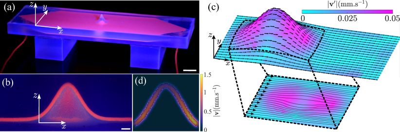
Figure 1: (a) Picture of a Hele-Shaw cell made of UV curable resin. It includes a localized curvature heterogeneity in the form of Gaussian bump located at the center of the channel. The device is filled with UV fabric paint for visualization purpose. ($h_{0}=3$ mm, $\sigma_{x}=\sigma_{y}=1.5$ mm). Scale bar: $8~{}\rm mm$. (b) 3D print of a half device. This side view of the channel shows that the gap between the two walls is constant even in the curved regions. Scale bar: $1~{}\rm mm$. (c) Top: Three-dimensional reconstruction of the velocity field perturbed by a Gaussian bump with $h_{0}=3$ mm, $\sigma_{x}=\sigma_{y}=1.5$ mm. The color indicates the magnitude of the flow perturbation $\mathbf{v^{\prime}}$ . Bottom: Corresponding streamlines projected in the $(x,y)$-plane. (d) Flow field measured across the channel gap. The black arrows show that the direction of the flow is tangent to the midsurface. The color indicates the magnitude of the velocity field. It has locally a Poiseuille shape. Note that the magnitude of the gap-averaged flow depends on the local geometry of the midsurface. This observation is consistent with the magnitude of $\mathbf{v}^{\prime}$ showed in panel (c).

We perform our experiments in three-dimensional (3D) printed microfluidic channels, see Fig. 1(a). We make our channels with a Formlab3 printer and use a transparent photocurable resin (Formlab clear), see also the Supplemental Material (SM) SM . In all our experiments the Hele-Shaw cells have a length $L=120~{}\rm mm$ and a width $W=38~{}\rm mm$. We however perturb the geometry by adding a Gaussian bump at the center of the device as exemplified in Fig. 1(a). We stress that the gap of the cells is constant across the whole device, $e=450~{}$µm, see Fig. 1(b). The geometry of the channels is fully captured by the shape of their midsurface. We define it by the height field $h(x,y)=h_{0}\exp[-x^{2}/(2\sigma_{x}^{2})-y^{2}/(2\sigma_{y}^{2})]$, where $\sigma_{x},\ \sigma_{y}$ are the widths of the bump in the $x$- and $y$-directions respectively.

We drive the flow with a piezoelectric pressure controller Elveflow OB1 MK4 and image it with a Hamamatsu ORCA-Quest qCMOS camera mounted on a Nikon AZ$100$ microscope with a $1.2$ zoom. We measure the velocity field averaged over the depth of field of our objective in the $(x,y)$ plane. To do so, we use a water-glycerol mixture ($20~{}\rm vol\%$) seeded with Fluorescent colloidal particles of diameter $4.8$ µm (Thermo Scientific G0500), and perform standard Particle Imaging Velocimetry Thielicke and Sonntag (2021). Knowing $h(x,y)$, we can then project the velocity back on the tangent plane and reconstruct the full 3D structure of the flow $\mathbf{v}(x,y)$ on the curved surface. In Fig. 1(c), we can see that the streamlines bend around the bump.

To better quantify these flow perturbations, we define $\mathbf{v}^{\prime}=\mathbf{v}-\mathbf{v}_{0}$, where, $\mathbf{v}_{0}=v_{0}\hat{\mathbf{x}}$ is the uniform flow measured at large distance from the bump. Fig. 2(a) shows that $\mathbf{v}^{\prime}$ has a clear dipolar symmetry, akin to the flow around a fixed obstacle in a flat channel Guyon et al. (2015). Given this symmetry, and the Laplacian nature of the hydrodynamic problem, one would expect $|\mathbf{v}^{\prime}|$ to decay algebraically with $\rho=\sqrt{x^{2}+y^{2}}$, the distance to the apex of the bump, ($|\mathbf{v}^{\prime}|\propto 1/\rho^{2}$, like the electric field induced by a charge dipole in two dimensions) Beatus et al. (2006); Cui et al. (2004), see also SM SM . This prediction is however at odds with our measurements. The flow perturbations are exponentially localized in space within the footprint of the bump. This atypically fast decay is better seen in Fig. 2(b), where we plot the $y$-component of $\mathbf{v}^{\prime}$ as a function of $x$.

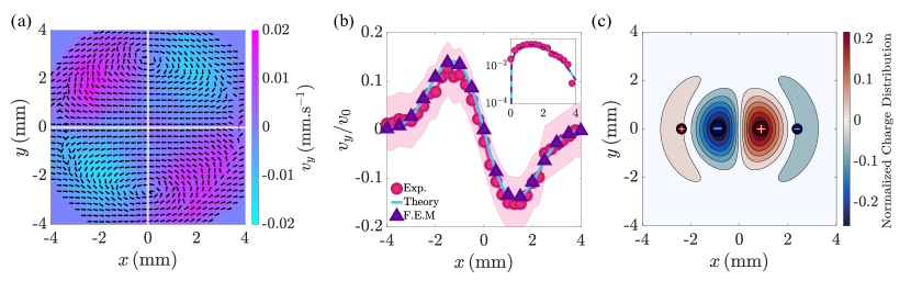
Figure 2: Isotropic bumps. (a) Experiments. Planar projection of $\mathbf{v}^{\prime}$ in the vicinity of an axisymmetric Gaussian bump with parameters $h_{0}=2.25~{}$mm and $\sigma_{x}=\sigma_{y}=1.5$ mm. Away from the bump the fluid flows at a velocity $v_{0}=120$ µ$\rm m.s^{-1}$ along the $x$-direction. The velocity field has the same angular symmetry as the electric field induced by a charge dipole antiparallel to the unperturbed flow. (b) Experiments, theory and simulations. $y$-component of the velocity perturbation $v_{y}^{\prime}$ for an axisymmetric Gaussian bump ($h_{0}=3~{}$mm, $\sigma=\sigma_{x}=\sigma_{y}=1.5$ mm). $v_{y}^{\prime}$ is plotted as a function of the coordinate $x$ in the direction of the unperturbed flow. The velocity is measured at $y/\sigma=0.78\pm 0.09$. The theoretical results derived from conformal theory in an infinite channel, and from FEM simulations in a finite channel are in excellent agreement with our measurements. Inset: log-lin plot of the same data. (c) Theory. Color map of the equivalent normalized charge distribution $\kappa\sigma^{3}\lambda/(v_{0}h_{0}^{2})$. It roughly corresponds to the superposition of two antiparallel dipoles that exactly cancel out.

This counter intuitive effect begs for a theoretical explanation. To address this question analytically and numerically, we first need to write the covariant generalizations of Darcy’s law and mass conservation on a curved surface. They take the compact form

$$v^{\alpha}=-\kappa g^{\alpha\beta}\partial_{\beta}p,$$ (3)

$$\frac{1}{\sqrt{g}}\partial_{\alpha}\left(\sqrt{g}v^{\alpha}\right)=0.$$ (4)

$v^{\alpha}$ ($\alpha=x,\ y$) is the $\alpha$-component of the velocity field in the local basis $(\mathbf{e_{x}},\ \mathbf{e_{y}})$ of the tangent plane to the midsurface, $\mathbf{e_{x}}=\mathbf{\hat{x}}+\mathbf{\hat{z}}\,\partial_{x}h$, $\mathbf{e_{y}}=\mathbf{\hat{y}}+\mathbf{\hat{z}}\,\partial_{y}h$, and $g_{\alpha\beta}=\delta_{\alpha\beta}+\partial_{\alpha}h\,\partial_{\beta}h$ is the associated metric. Combining these two equations we find that the pressure field $p$ obeys the Laplace-Beltrami equation: $(1/\sqrt{g})\partial_{\alpha}(\sqrt{g}g^{\alpha\beta}\partial_{\beta}p)=0$, see SM for a detailed derivation of the above equations SM . Equations (3) and (4) tell us that any local change in the metric should alter Darcy’s flows.

When the geometry of the channel is modified by an axisymmetric bump $h(\rho)$, we can compute the pressure and flow fields by taking advantage of the conformal invariance of the Laplace-Beltrami operator Bazant (2004). We consider a single bump on an infinite surface and a uniform flow away from the bump. We can then flatten the surface using a global conformal map described by the conformal factor $\Omega(\rho)$, solve Laplace’s equation in the plane, and finally apply the inverse transform to compute the pressure and velocity fields on the bumpy surface, see SM SM . Regardless of the specific shape of the bump, the conformal factor is given by Vitelli and Nelson (2004):

$$\Omega(\rho)=\exp\left[\int_{\rho}^{+\infty}\frac{\mathrm{d}\varrho}{\varrho}\left(\sqrt{1+h^{\prime}(\varrho)^{2}}-1\right)\right].$$ (5)

Fig. 2(b) shows that our analytical solution is in excellent agreement with our experimental findings. This agreement establishes that the measured deviation to a uniform flow field originates from curvature heterogeneities. We also note that conformal invariance readily informs us on the range of the flow perturbations. Isotropic bumps are conformally flat, in other words we can deform them into a planar surface by applying a global map that solely involves local dilations of the curved metric. Away from the bump, the local dilation factor becomes vanishingly small and therefore the solution of Eqs. (3) and (4) reduces to the uniform flow of a flat Hele-Shaw cell. The decay of $|\mathbf{v}^{\prime}|$ is therefore set by the decay of $\Omega(\rho)-1$: for Gaussian bumps $\mathbf{v}^{\prime}$ is exponentially localized in space.

To understand deeper the singular range of the flows around axisymmetric curvature heterogeneities, we now take advantage of an electrostatic analogy. In the limit of small aspect ratio $a=h_{0}/\sigma\ll 1$ ($\sigma=\sigma_{x}=\sigma_{y}$), we expand Eqs. (3) and (4) to second order in $a$ and find that the lowest-order correction to the pressure field satisfies Poisson’s equation:

$$\Delta p^{(2)}=-\kappa^{-1}(\mathbf{v}_{0}\cdot\bm{\nabla}h)\Delta h,$$ (6)

with $p^{(2)}(x,y)\to 0$ when $x,y\to\infty$ (see also SM SM for a detailed derivation). Computing the first correction to the pressure field is thus equivalent to finding the electric potential induced by a charge distribution $\lambda=\kappa^{-1}(\mathbf{v}_{0}\cdot\bm{\nabla}h)\Delta h$. To gain some intuition about the form of the pressure fluctuations, we plot the charge distribution $\lambda(x,y)$ in Fig. 2(c). In the far-field limit, the equivalent charge distribution can be seen as the sum of two dipoles pointing in opposite directions as the signs of the local slope $(\mathbf{v}_{0}\cdot\bm{\nabla}h)=v_{0}\partial_{x}h$, and mean curvature $\Delta h$, change once and twice respectively across the bump. The first dipole is formed by strong charges separated by a small distance, while the second dipole is formed by weaker charges separated by a larger distance, see Fig. 2(c).

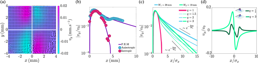
Figure 3: Anisotropic bumps. (a) Experiments. Planar projection of $\mathbf{v}^{\prime}$ in the vicinity of an anisotropic Gaussian bump with parameters $h_{0}=3.5$mm, $\sigma_{x}=1.5$ mm and $\sigma_{y}=4.5$ mm. The streamlines of the velocity field retain a dipolar symmetry. (b) Experiments and simulations. Log-lin plot of the perturbation to the mean flow for an isotropic Gaussian bump with parameters $h_{0}=3~{}$mm, $\sigma_{x}=\sigma_{y}=1.5$ mm and for an anisotropic bump with parameters $h_{0}=3.5$mm, $\sigma_{x}=1.5$ mm, $\sigma_{y}=4.5$ mm as a function of the coordinate $x$ in the direction of the unperturbed flow for $y/\sigma_{y}=0.78\pm 0.09$. We plot both the experimental and FEM results. (c) FEM simulations. Log-lin plot of the perturbation to the mean flow for four diffent anisotropic bumps in channels of two different widths $W$. The decay of $|\mathbf{v^{\prime}}|$ is set by the shape of the isotropic bump, by contrast $|\mathbf{v^{\prime}}|$ decays much slower for anisotropic bumps. In the far-field limit, the algebraic decay is exponentially screened over a distance set by the channel width. (d) FEM simulations. Lin-lin plot of the perturbation to the mean flow for two anisotropic bumps pointing in orthogonal directions, see sketches, opposite anisotropies obtained from FEM simulations. The sign of the far-field perturbation changes when the orientation of the main axis of the bump exceeds $45^{\circ}$.

For any axisymmetric bump, the two dipoles cancel out exactly. To see this, we can compute the net dipole associated with the charge distribution $\mathbf{P}=\iint\mathrm{d}x\,\mathrm{d}y\,\lambda(x,y)\left(x\,\mathbf{\hat{x}}+y\,\mathbf{\hat{y}}\right)$, and find

$$\mathbf{P}=\frac{\pi v_{0}h_{0}^{2}}{4\kappa}\left(\frac{\sigma_{x}}{\sigma_{y}}-\frac{\sigma_{y}}{\sigma_{x}}\right)\mathbf{\hat{x}}.$$ (7)

$\mathbf{P}$ vanishes when $\sigma_{x}=\sigma_{y}$, as well as all higher-order multipoles as shown in SM SM . Therefore, despite the existence of a non-trivial charge distribution, the far-field correction to the pressure around an isotropic bump cannot be captured by any multipolar expansion. The fluctuations of the flow field require some more attention. $\mathbf{v}^{\prime}(\mathbf{r})$ has indeed both a kinematic and a dynamic origin which are both impacted by curvature. At a perturbative level $\mathbf{v}^{\prime}=v_{0}g^{(2)}:\mathbf{e_{x}}-\kappa\left[\partial_{x}p^{(2)}\mathbf{e_{x}}+\partial_{y}p^{(2)}\mathbf{e_{y}}\right]$, where $g^{(2)}$ is the second-order correction to the inverse metric. The first term is a mere kinematic correction that stems from the projection of the unperturbed flow field on the tangent plane. The second term is specific to Darcy’s flows and may carry non-local perturbations to the velocity field. It is analogous to the electric field induced by the charge distribution $\lambda$. When $\sigma_{x}=\sigma_{y}$ both terms vanish in the far-field limit: all curvature-induced flows are screened past the footprint of the bump.

We note in passing that the agreement between our experimental observations and our theory justifies the relevance of our two-dimensional Laplacian theory despite the weak scale separation between the gap size and the spatial extent of the bump. With hindsight this agreement is however not surprising as typical Brickman’s corrections would result in corrections to the velocity field of the order of $[e/(\pi\sigma_{x})]^{2}\approx 10^{-2}$ Zeng et al. (2003).

We now move to our second central result, as clearly seen in Eq. (7), our results heavily rely on rotational symmetry. We therefore need to address the impact of curvature anisotropy, which would exist in any natural setting. At a perturbative level, the electrostatic analogy tells us that the flow perturbations should be long-ranged regardless of the specific functional form of $h$, $|\mathbf{v^{\prime}}|$ should decay as $1/\rho^{2}$, see Eq. (7). To assess whether this prediction holds beyond perturbation theory, it would be tempting to use the same theoretical tools as above. Namely to look for a global conformal transformation that would map anisotropic bumps onto planar domains Blanc and Fiala (1941). We indeed know that simple conformal maps transform anisotropic domains into isotropic ones, such as the celebrated Joukowski transform in the context of fluid mechanics. These maps should however cause long-range correlations in the $\mathbf{v}^{\prime}(x,y)$ field, as they typically involve inversions, which are non-local transformations. There is therefore no reason to expect any geometrical screening of the curvature-induced perturbations.

To further confirm our reasoning, we first conduct experiments in channels deformed by Gaussian bumps with $\sigma_{y}>\sigma_{x}$ and measure $\mathbf{v}^{\prime}$, see Fig. 3. We find that the angular symmetry of the perturbation remains mostly dipolar, see Fig. 3(a). But, Fig. 3(b) shows that the perturbation induced by anisotropic bumps extends as expected over much larger distances.

However, unlike our theoretical prediction, $|\mathbf{v}^{\prime}|$ still decays exponentially. The finite width of our channels explains this much simpler screening effect. Using again our electrostatic analogy, the two side walls of the channel acts as two conductors which screen the electric potential induced by a point dipole over a distance $W/(2\pi)$, see also SM SM . To quantitatively check our reasoning, we perform FEM simulations of Eqs. (3) and (4), see SM SM . Fig. 3(b) shows an excellent agreement with our measurements, and Fig. 3(c) confirms that the far-field decay of the flow is not set by the bump geometry but by the channel width only.

As a last comment, we note that our electrostatic analogy informs us on the sign of the far-field perturbation as well. As $\mathbf{P}\propto\mathbf{\hat{x}}$ when $\sigma_{x}>\sigma_{y}$, and $\mathbf{P}\propto-\mathbf{\hat{x}}$ otherwise, the far-field perturbation should be positive (resp. negative) when the long axis of the bump makes a smaller angle with the $y$-axis (resp. $x$-axis). Our FEM simulations again confirm that this last prediction holds even in the limit of high bumps, see Fig. 3(d).

To conclude, we have shown that unlike Stokes flows Davidovitch and Klein (2022), static curvature heterogeneities generically deform the streamlines of Darcy’s flows. Combining microfluidic experiments and theory we have revealed that curvature anisotropy acts as a singular perturbation to potential flows. Using a robust electrostatic analogy we have explained why the flow distortions induced by isotropic bumps are screened while vanishingly-small curvature asymmetries could bend the streamlines over system-spanning scales. We hope that our findings will stimulate a deeper investigation of the role of curvature heterogeneities on a broader class of Laplacian phenomena ranging from superfluid film flows to transport in fractured rocks and Ohmic transport in wrinkled two-dimensional conductors. We also expect our results to be relevant to non-Laplacian problems that can be solved using conformal mappings, such as advection-diffusion in potential flows, electrochemical transport Bazant (2004), and possibly stress propagation and adhesion pattern formation in elastic films Mitchell et al. (2017); Hure et al. (2011).