Bootstrap test procedure for variance components in nonlinear mixed effects models in the presence of nuisance parameters and singular Fisher Information Matrix

Abstract

We examine the problem of variance components testing in general mixed effects models using the likelihood ratio test. We account for the presence of nuisance parameters, i.e. the fact that some untested variances might also be equal to zero. Two main issues arise in this context leading to a non regular setting. First, under the null hypothesis the true parameter value lies on the boundary of the parameter space. Moreover, due to the presence of nuisance parameters the exact location of these boundary points is not known, which prevents from using classical asymptotic theory of maximum likelihood estimation. Then, in the specific context of nonlinear mixed-effects models, the Fisher information matrix is singular at the true parameter value. We address these two points by proposing a shrinked parametric bootstrap procedure, which is straightforward to apply even for nonlinear models. We show that the procedure is consistent, solving both the boundary and the singularity issues, and we provide a verifiable criterion for the applicability of our theoretical results. We show through a simulation study that, compared to the asymptotic approach, our procedure has a better small sample performance and is more robust to the presence of nuisance parameters. A real data application is also provided.

1 Introduction

Mixed effects models are a powerful statistical tool to model longitudinal studies with repeated measurements or data with an underlying unknown latent structure as hierarchical data. There are many fields of applications, e.g. pharmacokinetic-pharmacodynamic [8], medicine [9], agriculture [39], ecology [7], psychology [29] or educational and social sciences [20]. These models allow to take into account two types of variabilities, between different individuals in a population and between several measurements made on the same individual, also called inter and intra variabilities. These are modeled by two types of effects: on the one hand, random effects that vary from one individual to another, and on the other hand, fixed effects, common to all individuals in the population (see [32], [15]).

From a modeling point of view, being able to distinguish among all effects those that can be modeled as fixed effects would allow to reduce the number of model parameters. This would also help to better identify the processes that are at the origin of the variability observed in the population. Two main approaches have been developed to tackle this task. On the one hand, some authors suggested methods based on variable selection, using a Bayesian procedure as in [13] or a penalized likelihood approach as in [27] or [22]. Specific selection criteria for mixed-effects models were also developed by [36, 23] and [16]. On the other hand, other authors focused on hypothesis testing for the nullity of some variance components of the random effects. Such a test is equivalent to comparing two nested models, and standard tools to address this question include the likelihood ratio, the score and the Wald tests statistics [37]. However two issues arise when testing the nullity of variance components, that prevent from using the usual asymptotic results of [38]. The first issue results from the true value of the variance parameter lying on the boundary of the parameter space, while the second is due to the singularity of the Fisher information matrix.

As far as the boundary issue is concerned, several authors studied the asymptotic of the likelihood ratio test statistic in this context. [14], [12], [33] derived the asymptotic distribution of the likelihood ratio test statistic in specific cases. [2], [34] gave a more general way of dealing with hypothesis testing when the true parameter is not constrained to be an interior point of the ambient space. In the context of mixed effects models, [4] derived the asymptotic distribution of the likelihood ratio test statistic for testing that any subset of the variances of the random effects is null. However, most of these references assume that the untested parameters do not lie on the boundary of the parameter space. When this is the case, the asymptotic distribution of the likelihood ratio test statistic is intractable as it depends on the unknown location of these nuisance parameters on the boundary [33]. Therefore, procedures that do not involve the asymptotic distribution of the test statistic can be preferred. In particular, resampling methods such as bootstrap and permutations are powerful tools to address this issue. In addition, these methods are usually more robust in small samples context. [35] proposed a bootstrap-based score test in the context of generalized linear mixed models with one single random effect. [17] proposed a permutation-based test for any subset of the covariance matrix of the random effects in linear mixed models. The latter method is very easy to use in practice but is restricted to the context of linear models. The former requires the computation of the Fisher information matrix, which can be heavy in practice, especially in the context of nonlinear models. Moreover, the presence of nuisance parameters on the boundary of the parameter space is not considered in the aforementioned works, even though it can be a source of inconsistency for the proposed bootstrap procedures. Indeed, as discussed in [5], and highlighted in [3], the bootstrap is known to be inconsistent when the true parameter value is a boundary point. When estimating the expectation of a Gaussian distribution, restricted to be nonnegative, [3] proposed a parametric procedure that shrinks the parameter used to generate the bootstrap data near the boundary. Following this idea, [11] proposed a more general parametric bootstrap test procedure based on the Likelihood Ratio Test statistic with parameters lying on the boundary. Their method consists in shrinking the bootstrap parameter in order to accelerate its rate of convergence toward the boundary.

The second issue is the singularity of the Fisher information matrix that arises specifically in the context of mixed effect models, as discussed in [18]. Following the development of [25] to derive the new asymptotic distribution of the likelihood ratio test statistic, we show that this singularity issue is another source of inconsistency of the bootstrap procedure.

In this work we propose a shrinked parametric bootstrap test procedure for variance components in nonlinear mixed effects models that addresses the two issues mentioned above. We show that given an appropriate choice of the bootstrap parameter, the procedure is consistent as the number of individuals grows to infinity. Our contribution is twofold: first, our procedure can be applied to linear, generalized linear and nonlinear models, and second, it takes into account the presence of nuisance parameters at unknown locations. We also provide a verifiable criterion to check the required regularity conditions. Finally, we illustrate our results on simulated and real data, exhibiting the good finite sample properties of the procedure and its applicability in practice.

Section 2 presents the mixed effects model that is considered in this article and describes the proposed shrinked parametric bootstrap procedure. Section 3 is dedicated to the theoretical study of the proposed procedure, and shows its consistency first in the independent and identically distributed setting and then in the more general independent but not identically distributed setting. Section 4 presents a simulation study that illustrates the performance of the test in different models and with varying sample sizes. A real data application is also presented. All the proofs and additional developments can be found in the supplementary material.

2 Proposed methodology

2.1 Mixed effects models

Consider $N$ individuals each measured $J_{i}<J$ times, where $N$ and $J_{i}$ are nonnegative integers. We denote by $y_{ij}$ ($i=1,...,N;j=1,...,J_{i}$) the $j$th observation of the $i$th individual and we define $y_{i}=(y_{i1},\dots,y_{iJ_{i}})$ and $y_{1:N}=(y_{1}^{T},\dots,y_{N}^{T})$. In the sequel, $\mathcal{L}_{p}^{+}$ denotes the space of lower triangular matrices of size $p\times p$ with positive diagonal coefficients, $\mathbb{S}^{p}_{+}$ denotes the space of symmetric, positive semi-definite $p\times p$ matrices, $I_{p}$ is the identity matrix of size $p\times p$, $[A]_{ij}$ is the element on the $i$th line and $j$th column of matrix $A$, and $\mathcal{N}(\mu,V)$ denotes the multivariate Gaussian distribution with expectation $\mu\in\mathbb{R}^{p}$ and covariance matrix $V$ of size $p\times p$. We consider the following nonlinear mixed effects model

$$\left\{\begin{array}[]{ll}y_{ij}&=g(x_{ij},\beta,\Lambda\xi_{i})+\varepsilon_{ij}\quad\varepsilon_{ij}\sim\mathcal{N}(0,\sigma^{2})\\ \xi_{i}&\sim\mathcal{N}\left(0,I_{p}\right)\\ \end{array}\right.,$$ (1)

where $(\xi_{i})_{i=1,\dots,N}$ and $(\varepsilon_{ij})_{i=1,..,N,j=1,...,J_{i}}$ are mutually independent random variables, $g$ is a known nonlinear function, $x_{ij}$ gathers all the covariates of the $j$th observation of the $i$th individual, $\beta\in\mathbb{R}^{b}$ is the vector of fixed effects, $\Lambda\in\mathcal{L}_{p}^{+}$ is a scaling parameter for random effect $\xi_{i}$, and $\sigma^{2}$ is the positive noise variance.

Remark 1

The covariance matrix of the scaled random effect $b_{i}=\Lambda\xi_{i}$ is equal to $\Gamma=\Lambda\Lambda^{T}$ which is positive semi-definite. Therefore, a natural choice for $\Lambda$ is the lower triangular matrix in the Cholesky decomposition of the scaled random effects covariance matrix. Moreover, by constraining the diagonal coefficients of $\Lambda$ to be nonnegative, $\Lambda$ is uniquely defined. This decomposition is used for instance in [13]. _□

Remark 2

The definition of model (1) is slightly more general than the usual terminology of mixed effects models [32, p. 306] that defines $y_{ij}=g(v_{ij},\phi_{i})+\varepsilon_{ij}$, with $\phi_{i}=A_{ij}\beta+B_{ij}b_{i}$ the $i$th individual parameter, $\beta$ the vector of fixed effects associated with random effect $b_{i}\sim\mathcal{N}(0,\Gamma)$, and where $v_{ij}$, $A_{ij}$ and $B_{ij}$ are known covariates. Model (1) covers this definition by taking $x_{ij}=(v_{ij},B_{ij},A_{ij})$ and $b_{i}=\Lambda\xi_{i}$. A more detailed development of the differences between those two parameterizations is given in section (7.1) of the supplementary material. _□

Let us denote by $\theta=(\beta,\Lambda,\sigma^{2})$ the unknown vector of model parameters taking values in $\Theta$, by $f_{i}(\cdot;\theta)$ the density of the $i$th individual response $y_{i}$ given a parameter $\theta\in\Theta$, by $f_{i}(y_{i};\xi_{i},\theta)$ the conditional density of $y_{i}$ given the random effect $\xi_{i}$ and a parameter $\theta$, and by $\pi_{p}(\cdot)$ the density of the $p$-dimensional standard Gaussian density. With these notations we can define the log-likelihood of the model given the $N$-sample $y_{1:N}$ by

$$l(\theta;y_{1:N})=\log\{L_{\theta}(y_{1:N})\}=\log\{\prod_{i=1}^{N}f_{i}(y_{i};\theta)\}=\sum_{i=1}^{N}\log\{\int f_{i}(y_{i};\xi_{i},\theta)\pi(\xi_{i})d\xi_{i}\}$$ (2)

We consider the marginal likelihood defined as the complete likelihood integrated over the distribution of the random effects, since the random effects $\xi_{i}$ are unobserved.

With our notations, the distribution of the random effects $\xi_{i}$ does not depend on any parameter, contrary to the common case where the random effects are defined as the scaled version $b_{i}$. With the latter definition, the distribution of the latent variables depends on $\Lambda$, and is not defined on the entire parameter space since we only constrain $\Gamma=\Lambda\Lambda^{T}$ to be positive semi-definite. When dealing with linear models, since the variance of the random effects adds up with the noise variance, the fact that some diagonal components in $\Gamma$ are null is not an issue. However, the change of variable $b_{i}=\Lambda\xi_{i}$ is a $\mathcal{C}^{1}$ diffeomorphism if and only if the diagonal coefficients of $\Lambda$ are nonnegative. Without this assumption the two parametrizations are no longer equivalent as illustrated in the supplementary material (see section 7.1). Our parametrization is similar to the so-called reparametrization trick proposed by [28] to train variational autoencoders with back-propagation.

2.2 Variance components testing

Let $r\in\{1,\dots,p\}$ be the number of variances to be tested. Without loss of generality we assume that we test the nullity of the last $r$ variances in $\Gamma=\Lambda\Lambda^{T}$. Therefore let us consider the following block matrix notation

$$\Lambda=\left(\begin{array}[]{c|c}\Lambda_{1}&0_{(p-r)\times r}\\ \hline\cr\Lambda_{12}&\Lambda_{2}\end{array}\right),$$

where $\Lambda_{1}\in\mathcal{L}_{p-r}^{+}$, $\Lambda_{2}\in\mathcal{L}_{r}^{+}$ and $\Lambda_{12}\in\mathcal{M}_{r\times(p-r)}\left(\mathbb{R}\right)$. We write $\theta_{0}$ the true parameter on which we consider the following test :

$$H_{0}:\theta_{0}\in\Theta_{0}\hskip 8.5359pt\text{against}\hskip 8.5359ptH_{1}:\theta_{0}\in\Theta,$$ (3)

where

$$\Theta_{0} =\{\theta\in\mathbb{R}^{q}\mid\beta\in\mathbb{R}^{b},\Lambda_{1}\in\mathcal{L}_{p-r}^{+},\Lambda_{2}=0,\Lambda_{12}=0,\sigma^{2}\in\mathbb{R}_{*}^{+}\},$$

$$\Theta =\{\theta\in\mathbb{R}^{q}\mid\beta\in\mathbb{R}^{b},\Lambda\in\mathcal{L}_{p}^{+},\sigma^{2}\in\mathbb{R}_{*}^{+}\}.$$

Remark 3

We do not impose the diagonal of $\Lambda_{1}$ to be strictly non-negative, which enables the case where some untested variances of the scaled random effects are in fact equal to zero. This will be discussed in more details in section (3.1) with the definition of nuisance parameters. _□

The likelihood ratio test statistic is defined as

$$\textsc{lrt}(y_{1:N})=-2\left(\underset{\theta\in\Theta}{\sup}\quad l(\theta;y_{1:N})-\underset{\theta\in\Theta_{0}}{\sup}\quad l(\theta;y_{1:N})\right).$$

In order to test (3) with a nominal level $0<\alpha<1$, we define the rejection region as $R_{\alpha}=\{\textsc{lrt}(y_{1:N})\geq q_{\alpha}\}$ with $q_{\alpha}$ being the $(1-{\alpha})$th quantile of the distribution of $\textsc{lrt}(y_{1:N})$. Unfortunately, this distribution is often intractable.

In the following section, we detail the proposed shrinked parametric bootstrap procedure to test (3).

2.3 Testing procedure

We propose a parametric bootstrap procedure using a bootstrap parameter ${\theta_{N}^{*}}$ and $B\in\mathds{N}^{*}$ bootstrap replications to test (3) with a type I error $0<\alpha<1$. As introduced in remark 3 and then detailed in section (3.1), some untested variances, at unknown locations, can be null. Therefore using $\hat{\theta}_{N}=(\hat{\beta}_{N},\hat{\Lambda}_{N},\hat{\sigma}_{N}^{2})$ the maximum likelihood estimator as a bootstrap parameter over $\Theta$ would fail to asymptotically mimic the true distribution of the likelihood ratio test statistic. Indeed there are elements in $\Lambda_{0}$ which are supposed to be zero, but that are non null in $\hat{\Lambda}_{N}$. Since we require that ${\theta_{N}^{*}}\in\Theta_{0}$, we use a shrinking parameter $c_{N}$ to fix to zero the diagonal parameters of $\Lambda$ that are smaller than $c_{N}$. The proposed algorithm is described in algorithm 1, and the theoretical justification of this shrinking procedure is described in section 3.

Input: $c_{N}>0$, $B\in\mathds{N}^{*}$, $0<\alpha<1$

Set ${\beta_{N}^{*}}=\hat{\beta}_{N}$, ${\Lambda_{N}^{*}}=\hat{\Lambda}_{N}$, and ${\sigma_{N}^{*}}^{2}=\hat{\sigma}_{N}^{2}$

Set $\Lambda_{2,N}^{*}=\Lambda_{12,N}^{*}=0$

Set $[\Lambda_{1,N}^{*}]_{mn}=[\hat{\Lambda}_{1,N}]_{mn}\mathds{1}_{[\hat{\Lambda}_{1,N}]_{mn}>c_{N}}$

For $b=1,...,B$

For $i=1,...,N$, draw independently $\varepsilon_{i}^{*,b}\sim\mathcal{N}(0,{\sigma_{N}^{*}}^{2}I_{J_{i}})$ and $\xi_{i}^{*,b}\sim\mathcal{N}(0,I_{p})$

Build the $i$th value of the $b$th bootstrap sample $y_{i}^{*,b}=g(x_{i},{\beta_{N}^{*}},{\Lambda_{N}^{*}}\xi_{i}^{*,b})+\varepsilon_{i}^{*,b}$

Compute the likelihood ratio statistic $\textsc{lrt}(y^{*,b}_{1:N})$

Compute the bootstrap $p$-value as $p_{boot}=\frac{1}{B}\sum_{b=1}^{B}\mathds{1}_{\textsc{lrt}(y^{*,b}_{1:N})>\textsc{lrt}(y_{1:N})}$

Reject $H_{0}$ if $p_{boot}<\alpha$

Algorithm 1 Shrinked parametric bootstrap for variance components testing

The next section is dedicated to the asymptotic validity of this testing procedure.

3 Theoretical results

3.1 Notations and theoretical setting

In this section we are interested in the theoretical consistency of the bootstrap procedure presented in section 2.3. We consider the asymptotic as the number of individuals $N$ grows to infinity, while the number of measurements per individual remains fixed and bounded by some value $J$. We denote by $\theta_{0}\in\Theta_{0}$ the true value of the parameter, such that the density of the response $y_{1:N}$ is $L_{\theta_{0}}(y_{1:N})$. We denote by $E\{T(y_{1:N})\}$ the expectation of any measurable function $T$ of $y_{1:N}$ if there is no confusion about the distribution of $y_{1:N}$. Otherwise we specify $E_{\theta}\{T(y_{1:N})\}$ to emphasize that the expectation is with respect to the density $L_{\theta}(y_{1:N})$, for any $\theta\in\Theta$. As commonly used in the bootstrap literature, we denote by $X^{*}$ the bootstrap version of a random variable $X$. We write $E^{*}\{T(y_{1:N}^{*})\}=E_{{\theta_{N}^{*}}}\{T(y_{1:N}^{*})\mid y_{1:N}\}$. Similarly, for any measurable subset $A$ we write $\textnormal{pr}^{*}\{T(y_{1:N}^{*})\in A\}=E_{{\theta_{N}^{*}}}\{\mathds{1}_{T(y_{1:N}^{*})\in A}\mid y_{1:N}\}$.

We want to show that the proposed bootstrap procedure is asymptotically valid which means that $\textsc{lrt}(y^{*}_{1:N})$ converges weakly in probability to the same limiting distribution as the one of $\textsc{lrt}(y_{1:N})$. More precisely, we want to show that, under some conditions, if there exists a random variable $\textsc{lrt}_{\infty}$ such that $\textsc{lrt}(y_{1:N})$ converges weakly to $\textsc{lrt}_{\infty}$ then for every $t\in\mathbb{R}$, as $N\rightarrow+\infty$, it holds in probability that

$$\textnormal{pr}^{*}\{\textsc{lrt}(y^{*}_{1:N})\leq t\}\longrightarrow\textnormal{pr}(\textsc{lrt}_{\infty}\leq t).$$ (4)

We also use the notations $o_{p}(1)$ and $O_{p}(1)$ for random sequences that respectively converge toward zero and are bounded in probability. More generally, this notation is used to compare two random sequences, using the definition of [37]. We also use their bootstrap versions $o_{p^{*}}$ and $O_{p^{*}}$ defined as follows: for a random quantity $X_{N}^{*}$ computed on the bootstrap data, $X_{N}^{*}=o_{p^{*}}(1)$ means that for any $\varepsilon>0$, $\textnormal{pr}^{*}(X_{N}^{*}>\varepsilon)\rightarrow 0$ in probability as $N\rightarrow+\infty$. Similarly $X_{N}^{*}=O_{p^{*}}(1)$ means that for any $\varepsilon>0$ there exists a real $M>0$ and an integer $N_{0}$ such that for all $N>N_{0}$, the event $\{\textnormal{pr}^{*}(\|X_{N}^{*}\|>M)<\varepsilon\}$ is arbitrary close to one in probability.

We now formalize what we call nuisance parameters. We suppose that, in addition to the last $r$ tested variances, $m$ untested variances are null. Without loss of generality we suppose that the last $m+r$ variances of the individual parameters are null therefore $\Lambda_{0}$ is of the form

$$\Lambda_{0}=\left(\begin{array}[]{c|c|c}\Lambda_{1}^{nonuis}&0_{(p-r-m)\times m}&0_{(p-r-m)\times r}\\ \hline\cr\Lambda_{12}^{nuis}&\Lambda_{1}^{nuis}&0_{m\times r}\\ \hline\cr\Lambda_{12,1}&\Lambda_{12,2}&\Lambda_{2}\\ \end{array}\right)=\left(\begin{array}[]{c|c|c}\Lambda_{1}^{nonuis}&0_{(p-r-m)\times m}&0_{(p-r-m)\times r}\\ \hline\cr 0_{m\times(p-r-m)}&0_{m\times m}&0_{m\times r}\\ \hline\cr 0_{r\times(p-r-m)}&0_{r\times m}&0_{r\times r}\\ \end{array}\right).$$

It is important to notice that in real life applications the $m$ rows inducing nuisance parameters are located at unknown positions in matrix $\Lambda$, and that the remaining $p-m-r$ variances are strictly non-negative which is equivalent to the diagonal coefficients of $\Lambda_{1}^{nonuis}$ being strictly non-negative.

We now split the parameter as $\theta=(\psi,\delta,\lambda)$, where $\lambda$ stands for all the coefficients of $\Lambda_{2}$ and $\Lambda_{12,2}$, $\delta$ represents the coefficients in $\Lambda_{1}^{nuis}$ and $\psi$ gathers all the remaining parameters. The dimension of $\lambda$ is $d_{\lambda}=r(r+1)/2+r(p-r-m)$, the dimension of $\delta$ is $d_{\delta}=m(m+1)/2+r\times m$ and the dimension of $\psi$ is $d_{\psi}=d_{\theta}-d_{\lambda}-d_{\delta}$. Moreover, $\theta_{0}=(\psi_{0},\delta_{0},\lambda_{0})=(\psi_{0},0_{d_{\delta}},0_{d_{\lambda}})$. Before introducing our results we first state a set of general conditions on the model that will be required in this work.

Assumption 1

i) $\Theta$ is compact, ii) the support of $y\mapsto f_{i}(y;\theta)$ does not depend neither on $\theta$, nor on $i$, iii) the model is identifiable, iv) for all $i\in\mathds{N},y\in\mathds{R}^{J}_{i}$, $\xi\in\mathds{R}^{p}$ the conditional likelihood $\theta\mapsto f_{i}(y;\xi,\theta)$ is 4-times differentiable on the interior of $\Theta$, and directional derivatives exist on the boundary, v) each partial derivative of $\theta\mapsto f_{i}(y;\xi,\theta)$ is bounded by a positive function which does not depend on $\theta$ and is integrable with respect to the distribution of the random effects.

Remark 4

The compactness assumption is not verified for $\Theta$. However in practice it only requires that $\sigma^{2}\geq\rho$ for some non-negative number $\rho$ and that each component of $\theta$ is upper and lower bounded, which is reasonable in real data application. Assumptions ii) and iii) are usual in the context of maximum likelihood theory, iv) is needed to perform a Taylor expansion of the log likelihood and v) is needed to differentiate under the integral sign in (2). _□

The following proposition induces that if the Fisher Information Matrix exists, it will present blocks equal to zero, and will therefore be singular.

Proposition 1

Under assumption (1), for $k=0,1$, for all $i\in\mathds{N}$ and for all $y\in\mathbb{R}^{J_{i}}$, $\nabla^{2k+1}_{\delta}\log\{f_{i}(y;\theta_{0})\}=0_{d_{\delta}^{2k+1}}$ and $\nabla^{2k+1}_{\lambda}\log\{f_{i}(y;\theta_{0})\}=0_{d_{\lambda}^{2k+1}}$. In particular, $\textnormal{var}\{\nabla_{\delta}l(\theta;y_{1:N})\}=0_{d_{\delta}\times d_{\delta}}$ and $\textnormal{var}\{\nabla_{\lambda}l(\theta;y_{1:N})\}=0_{d_{\lambda}\times d_{\lambda}}$. _□

Remark 5

If $\theta\mapsto l(\theta;y_{1:N})$ admits higher order derivatives, the first part of Proposition 1 is true for every odds order derivatives. This comes from the null odds moments of the standard normal distribution of the random effects. _□

Remark 6

As shown in the proof of proposition 1, in section 7.2 of the appendix, by considering the $k$th column $[\Lambda]_{.k}=([\Lambda]_{1k},...,[\Lambda]_{pk})^{T}$ of $\Lambda$, for all $j=1,...,p$, $\partial l(\theta;y_{1:N})/\partial[\Lambda]_{jk}|_{[\Lambda]_{.k}=0_{p}}=0$. That explains why the coefficients of $\Lambda_{12,2}$ are part of the definition of $\lambda$. _□

3.2 Consistency of the bootstrap procedure in the identically distributed setting

We first deal with the simpler identically distributed case. In model (1) it corresponds to the case where $(x_{ij})_{j=1,...,J_{i}}$ are common to every individual $i$. The next section is devoted to extending the results to the non identically distributed setting presented before.

Before studying the consistency of the test procedure, we first need to ensure the consistency of the restricted (respectively unrestricted) maximum likelihood estimator, i.e. computed over $\Theta_{0}$ (respectively $\Theta$). We first state the regularity conditions required for the asymptotic theory that follows.

Assumption 2

$$i)\quad\underset{\theta^{\prime}\in\Theta}{\sup}\mathrm{E}_{\theta^{\prime}}\{\underset{\theta\in\Theta}{\sup} |\log f(y_{i};\theta)|^{2}\}<+\infty$$

$$ii)\quad\underset{\theta^{\prime}\in\Theta}{\sup}\mathrm{E}_{\theta^{\prime}}\{\underset{\theta\in\Theta}{\sup} \|\nabla_{\theta}\log f(y_{i};\theta)\|^{3}\}<+\infty$$

$$iii)\quad\underset{\theta^{\prime}\in\Theta}{\sup}\mathrm{E}_{\theta^{\prime}}\{\underset{\theta\in\Theta}{\sup} \|\nabla^{2}_{\theta}\log f(y_{i};\theta)\|^{3}\}<+\infty$$

$$iv)\quad\underset{\theta^{\prime}\in\Theta}{\sup}\mathrm{E}_{\theta^{\prime}}\{\underset{\theta\in\Theta}{\sup} \|\nabla^{3}_{\theta}\log f(y_{i};\theta)\|^{2}\}<+\infty$$

$$v)\quad\underset{\theta^{\prime}\in\Theta}{\sup}\mathrm{E}_{\theta^{\prime}}\{\underset{\theta\in\Theta}{\sup} \|\nabla^{4}_{\theta}\log f(y_{i};\theta)\|^{2}\}<+\infty$$

Assumption (2) $i)$ is needed to ensure the consistency of the maximum likelihood estimators. Indeed it enables to derive a uniform law of large numbers. Assumptions $ii)$ and $iii)$ are similar to assumption (N8’) in [26]. It is required to apply a central limit theorem to the score function, and the pseudo score function $\tilde{S}_{N}(\theta)$ that appears in the quadratic expansion (see equation (21) in the appendix). Assumptions $iv)$ and $v)$ are needed to control the rest of the quadratic approximation. All the suprema are needed to control the consistency of the bootstrap distributions.

We now derive the consistency of the maximum likelihood estimators, following the result of [30].

Proposition 2

Under assumptions (1)–(2) $i)$ :

$$\arg\underset{\theta\in\Theta}{\max}\quad l(\theta;y_{1:N}) =\theta_{0}+o_{p}(1)$$

$$\arg\underset{\theta\in\Theta_{0}}{\max}\quad l(\theta;y_{1:N}) =\theta_{0}+o_{p}(1)$$

_□

A natural choice for the bootstrap parameter ${\theta_{N}^{*}}$ is the maximum likelihood estimator. However the bootstrap fails in presence of the nuisance parameters summarized in vector $\delta$. This is why care must be taken when choosing ${\delta_{N}^{*}}$. To explain and solve this issue we first need to derive the speed of convergence of the maximum likelihood estimator.

Proposition 3

Let $\hat{\theta}_{N}=(\hat{\psi}_{N},\hat{\delta}_{N},\hat{\lambda}_{N})$ and $\tilde{\theta}_{N}=(\tilde{\psi}_{N},\tilde{\delta}_{N},0_{d_{\lambda}})$ be respectively the unrestricted and restricted maximum likelihood estimators of $\theta$. Under assumptions (1) and (2) $(\hat{\psi}_{N},\tilde{\psi}_{N})=O_{p}(N^{-1/2}),(\hat{\delta}_{N},\tilde{\delta}_{N},\hat{\lambda}_{N})=O_{p}(N^{-1/4})$. _□

The usual way to derive the asymptotic distribution of the likelihood ratio statistic is to consider a quadratic approximation of the log-likelihood around the true value of the parameter, based on a second-order Taylor expansion. However in our case, due to the vanishing score property stated in proposition 1, this quadratic expansion is degenerate with respect to parameters $\delta$ and $\lambda$. Using a reparametrization of parameter $\theta$ as in [25], we obtain a new quadratic approximation based on a higher-order expansion of the log-likelihood. We then apply results from [2] and [34] to obtain an explicit formula for $\textsc{lrt}_{\infty}$. This new quadratic approximation involves a new matrix $\tilde{I}(\theta_{0})$ which plays the role of the Fisher information matrix, and which is defined explicitly in equation (21) of the supplementary material. This new matrix is no longer systematically degenerate, we can therefore state the usual assumption which must be verified case by case in real life applications.

Assumption 3

$\tilde{I}(\theta_{0})\succ 0$

Before showing that the proposed test procedure is consistent, we first need to show that in the boostrap world, if the bootstrap parameter is consistent, the bootstrap maximum likelihood estimators are, conditionally to the data, consistent.

Proposition 4

Under assumptions (1)–(2) $i)$, if ${\theta_{N}^{*}}$ the parameter used to generate the data is consistent, then :

$$\arg\underset{\theta\in\Theta}{\max}\quad l(\theta;y_{1:N}^{*}) =\theta_{0}+o_{p^{*}}(1)$$

$$\arg\underset{\theta\in\Theta_{0}}{\max}\quad l(\theta;y_{1:N}^{*}) =\theta_{0}+o_{p^{*}}(1).$$

_□

We can now state the main result of this article that guarantees the consistency of the bootstrap procedure.

Theorem 1

Under assumptions (1)–(3), if ${\theta_{N}^{*}}$ is chosen such that ${\theta_{N}^{*}}\in\Theta_{0}$, ${\theta_{N}^{*}}=\theta_{0}+o_{p}(1)$ and $N^{1/4}{\delta_{N}^{*}}=o_{p}(1)$ then as $N\rightarrow+\infty$, it holds in probability that

$$\textnormal{pr}^{*}\{\textsc{lrt}(y^{*}_{1:N})\leq t\}\longrightarrow\textnormal{pr}(\textsc{lrt}_{\infty}\leq t).$$ (5)

_□

A way of choosing ${\theta_{N}^{*}}$ that fulfills the hypothesis of theorem 1 is to follow the idea of [11] and shrinks the parameter toward 0. However here the rate of convergence of the shrinking parameter $(c_{N})$ is not the same due to the singularity issue. The following lemma gives a procedure to choose ${\theta_{N}^{*}}$ and justify the way it is chosen in algorithm 1.

Proposition 5

Let $(c_{N})_{N\in\mathds{N}}$ be a sequence such that $\underset{N\rightarrow+\infty}{\lim}c_{N}=0$ and $\underset{N\rightarrow+\infty}{\lim}N^{\frac{1}{4}}c_{N}=+\infty$. Let $\hat{\theta}_{N}=(\hat{\psi}_{N},\hat{\delta}_{N},\hat{\lambda}_{N})$ be a maximum likelihood estimator (restricted or not) of $\theta_{0}=(\psi_{0},0_{d_{\delta}},0_{\delta_{\lambda}})$. Under assumptions (1)–(3), by choosing ${\theta_{N}^{*}}=({\psi_{N}^{*}},{\delta_{N}^{*}},{\lambda_{N}^{*}})$ such that: $\forall k=1,..,d_{\psi}$ $\psi^{*}_{N,k}=\hat{\psi}_{N,k}\ \mathds{1}(\hat{\psi}_{N,k}>c_{N})$, $\forall k=1,..,d_{\delta}$ $\delta^{*}_{N,k}=\hat{\delta}_{N,k}\ \mathds{1}(\hat{\delta}_{N,k}>c_{N})$ and ${\lambda_{N}^{*}}=0_{d_{\lambda}}$ then, ${\theta_{N}^{*}}$ verifies the hypothesis of theorem 1. _□

As we do not know which parameters are part of $\delta$, it is important to deal with every potential nuisance parameters. This is why we also consider a shrinkage bootstrap parameter for $\psi$. In the proof of this proposition we show that the shrinkage does not change the limit of the estimate, but only speeds up its convergence toward $0$.

In addition to the boundary issue, the singularity is another source of inconsistency for the bootstrap procedure. As highlighted in the proof of theorem (1), this inconsistency comes from the polluting random variables due to the asymptotic distribution of $N^{\frac{1}{4}}{\delta_{N}^{*}}$, that does not appear in the asymptotic distribution of $LRT_{\infty}$. The shrinkage enables to enforce that $N^{\frac{1}{4}}{\delta_{N}^{*}}=o_{p}(1)$ and no longer $O_{p}(1)$.

3.3 Extension to the non identically distributed setting

As in the previous section we first derive the consistency of the maximum likelihood estimator. To do so, we need the regularity required in assumption (2) to hold uniformly over the different distributions of the individuals.

Assumption 4

We suppose that assumptions (2) $i)$–$v)$ hold uniformly over the different individuals $i\in\mathds{N}$.

In addition to that, as discussed in [26] an additional assumption is required to ensure the unicity of the maximum of the asymptotic objective function.

Assumption 5

For every $\theta\neq\theta_{0}$ :

$$\underset{N\rightarrow+\infty}{\lim}\frac{1}{N}\sum_{i=1}^{N}\mathrm{E}\left[\log\left\{\frac{f_{i}(y_{i};\theta)}{f_{i}(y_{i};\theta_{0})}\right\}\right]<0$$

.

Proposition 6

Under assumptions (1), (4) and (5), propositions 2 and 4 still hold in the non identically distributed case. _□

Following the same lines as in the last section the result of theorem 1 still holds.

Theorem 2

Under assumptions (1)–(5), if ${\theta_{N}^{*}}$ is chosen such that ${\theta_{N}^{*}}\in\Theta_{0}$, ${\theta_{N}^{*}}=\theta_{0}+o_{p}(1)$, i.e. ${\lambda_{N}^{*}}=0$ and $N^{\frac{1}{4}}{\delta_{N}^{*}}=o_{p}(1)$ then as $N\rightarrow+\infty$, it holds in probability that

$$\textnormal{pr}^{*}\{\textsc{lrt}(y^{*}_{1:N})\leq t\}-\textnormal{pr}(LRT_{N}\leq t)=o_{p}(1).$$ (6)

_□

3.4 Sufficient verifiable conditions for regularity assumptions

In this work we assume very strong regularity conditions on the model. Due to the integrated form of the likelihood in (2), it is often difficult to manipulate the quantities involved. [31] proposed some verifiable conditions under which the maximum likelihood estimators in nonlinear mixed models is strongly consistent. However in his work he considered that the true parameter is an interior point of the parameter space, and that the Fisher information matrix is nonsingular. Furthermore in our context the conditions required are even more difficult to verify as we deal not only with maximum likelihood estimator consistency but also with likelihood ratio and bootstrap statistic consistency.

We propose an analytical sufficient criterion that only depends on the regularity of the known function $g$ in model (1).

First we state a regularity condition on the derivatives of $g$.

Assumption 6

For all $k_{1}=0,...,4$ and $k_{2}\in\mathbb{N}$

$$\underset{i\in\mathds{N},j=1,...,J_{i}}{\sup}\mathrm{E}\{\quad\underset{\theta\in\Theta}{\sup}\|\nabla^{k_{1}}_{\theta}g(x_{ij},\beta,\Lambda\xi)\|^{k_{2}}\}<+\infty,\quad\xi\sim\mathcal{N}(0,I_{p}).$$ (7)

Remark 7

This assumption seems very strong but in practice it only requires that the derivatives of $g$ are not exponential in $\|\xi\|^{2}$ which is verified for almost every commonly used models. _□

We now state the regularity condition on $g$, which is the proposed criterion to be verified case by case in real life applications.

Assumption 7

for every $\varepsilon>0$, there exists a compact set $K\subset\mathds{R}^{p}$ such that

$$\forall\xi\in\mathds{R}^{p}\backslash K\quad\underset{i\in\mathds{N},,j=1,...,J_{i}}{\sup}\underset{\theta\in\Theta}{\sup}\quad\frac{\|g(x_{ij},\beta,\Lambda\xi)\|}{\|\xi\|}\leq\varepsilon.$$ (8)

Proposition 7

Suppose that assumption (1) holds, and that the function $g$ verifies assumption (6)–(7), then assumption (4) is verified. _□

4 Experiments

4.1 Simulation study

We denote by $\theta_{0}=(\beta_{0},\Lambda_{0},\sigma^{2}_{0})^{T}$ the true parameter used to generate the data. We use the notation $\beta_{k}$ for the $k$th component of the fixed effects vector $\beta$, and we write diag$(x_{1},...,x_{p})$ for a diagonal $p\times p$ matrix, with a diagonal being equal to $(x_{1},...,x_{p})^{T}$. When it is not explicitly written we consider diagonal matrices $\Lambda=\textnormal{diag}(\lambda_{1},...\lambda_{p})^{T}$. The same way we write $\xi_{i}=(\xi_{i1},...,\xi_{ip})^{T}$ for the vector of random effects. We consider a linear and a nonlinear mixed effects models, with a varying number of random effects to account for the presence of nuisance parameters. Results were obtained using the lme4 and saemix packages in R. Codes are available upon request from the first author.

We first consider the linear case. We denote by $m_{1}$ the linear model with two independent random effects, i.e. with $g(x_{ij},\beta,\Lambda\xi_{i})=\beta_{1}+\lambda_{1}\xi_{i1}+(\beta_{2}+\lambda_{2}\xi_{i2})x_{ij}$. We set $\beta_{0}=(0,7)^{T}$, $\lambda_{01}^{2}=1.3,\lambda_{02}=0$. In this model, we consider the test $H_{0}:\lambda_{2}=0$ against $H_{1}:\lambda_{2}\geq 0$. We then denote by $m_{2}$ the linear model with three independent random effects, i.e. with $g(x_{ij},\beta,\Lambda\xi_{i})=\beta_{1}+\lambda_{1}\xi_{i1}+(\beta_{2}+\lambda_{2}\xi_{i2})x_{ij}+(\beta_{3}+\lambda_{3}\xi_{i3})x_{ij}^{2}$. We set $\beta_{0}=(0,7,3)^{T}$, $\lambda_{01}^{2}=1.3,\lambda_{02}=0$, $\lambda_{03}=0$. In this model, we consider the test $H_{0}:\lambda_{3}=0$ against $H_{1}:\lambda_{3}\geq 0$, so that in this simulation $\lambda_{2}$ is a nuisance parameter. For the choice of the shrinkage bootstrap parameter, we set $c_{N}=0.28\approx 0.5\times 20^{-0.2}$. This choice is motivated by its theoretical definition, this parameter shrinks to zero the variances of the individual parameters $\beta_{2}+\lambda_{2}\xi_{i2}$ with a relative standard deviation lower than $4\%$. In both settings, we set $x_{ij}=j$, $J=5$ and $\sigma_{0}=1.5$. Finally, we denote by $m_{3}$ the linear model with $p=8$ random effects and a varying number $s$ of nuisance parameters, i.e. with $g(x_{ij},\beta,\Lambda\xi_{i})=\sum_{k=1}^{p}x_{ijk}\lambda_{k}\xi_{ik}$. Here we set $N=40$, $J_{i}=9$, $\sigma^{2}=2$, and every untested variance to $1$. Finally we draw independently the covariates from a normal distribution with mean 2 and standard deviation 0.5. We want here to illustrate the effect of an increasing number of nuisance parameters on the performance of the test. We use three different values for the shrinkage parameter $c_{N}\in\{0;0.24;0.9\}$. We chose those values to consider three cases: first $c_{N}=0$ is equivalent to the parametric bootstrap procedure without shrinkage, then $c_{N}=0.5\times 40^{-0.2}\approx 0.24$ shrinks most of the nuisance parameters toward 0, and finally $c_{N}=0.9$ shrinks systematically the nuisance parameters (as if we were using the true model), but can also shrink some non-zero variances of the model. We consider the test $H_{0}:\lambda_{1}=0$ against $H_{1}:\lambda_{1}\geq 0$.

Next, we consider the nonlinear logistic model with three random effects denoted by $m_{4}$, where

$$g(x_{ij},\beta,\Lambda\xi_{i})=\frac{\beta_{1}+\lambda_{1}\xi_{i1}}{1+\exp\left(-\frac{x_{ij}-(\beta_{2}+\lambda_{2}\xi_{i2})}{\beta_{3}+\lambda_{3}\xi_{i3}}\right)}.$$ (9)

We set $\beta_{0}=(200,500,150)^{T}$, $\lambda_{01}=\lambda_{02}=10$, $\lambda_{03}=0$ and $\sigma_{0}^{2}=5^{2}$. We set $(x_{i1},...,x_{iJ})=(50,287.5,525,762,1000,1100,1200,1300,1400,1500)$ for all $i$. In this model, we consider the test $H_{0}:\lambda_{3}=0$ against $H_{1}:\lambda_{3}\geq 0$.

First, we study the finite sample size properties of our procedure using models $m_{1}$, $m_{2}$ and $m_{4}$. We compute the empirical levels by generating $K$ datasets under the null hypothesis as described in the previous paragraph, and by computing the proportion of these datasets for which we reject the null hypothesis, for a nominal level $\alpha$ in $\{0.01,0.05,0.10\}$ and a sample size $N$ in $\{10,20,30,40,100\}$ for $m_{1}$, $N$ in $\{20,30,40\}$ for $m_{2}$ and $N=40$ for $m_{4}$. Results are given in tables 1, 2 and 3. We compare the empirical level of the test associated with our bootstrap procedure with those obtained using the asymptotic distribution which is a $0.5-0.5$ mixture between a Dirac distribution at zero and a chi–squared distribution with one degree of freedom [4]. We observe that the empirical levels obtained with our bootstrap procedure are closer to the nominal ones than those obtained with the asymptotic procedure, and that good results are already obtained for small values of $N$ in the linear case. As expected, our procedure exhibits better small sample size properties than the asymptotic procedure, both in the linear and the nonlinear cases. It is noteworthy to mention that the existing non-asymptotic test procedures such as the one proposed by [17] can not be used in the latter case since they rely on explicit expressions for the parameter estimates, hence requiring the linearity assumption. We also observe that the presence of nuisance parameters also deteriorate the asymptotic results. It is not a surprise as it modifies the true asymptotic distribution. However we observe that the standard parametric bootstrap procedure is robust to the presence of a single nuisance parameter, and so the choice of $c_{N}$ does not have a significant effect on this example. This must be due to the low number of nuisance parameters and the few number of parameters of the model.

Level $\alpha$	$N=10$		$N=20$		$N=30$		$N=40$		$N=100$		max sd
	boot	asym	boot	asym	boot	asym	boot	asym	boot	asym
1%	1.14	0.68	0.98	0.68	1.20	0.94	0.74	0.70	0.86	0.72	0.15
5%	5.20	3.64	5.22	3.82	5.74	4.30	4.86	3.94	5.26	4.50	0.33
10%	10.72	7.16	10.80	7.98	10.30	8.40	10.80	8.44	10.34	8.86	0.44

Table 1: Empirical levels (expressed as percentages) of the test that one variance is null in a linear model with two independent random effects, for $K=5000$ simulated datasets and $B=500$ bootstrap replicates. The last column gives the maximal standard deviation value obtained in each row

boot., parametric bootstrap procedure; asym., asymptotic procedure; sd, standard deviation .

Level $\alpha$	$N=20$		$N=30$		$N=40$		max sd
	boot	asym	boot	asym	boot	asym
1%	0.82	0.66	0.72	0.58	0.90	0.62	0.13
5%	4.46	3.54	3.96	3.28	4.14	3.08	0.29
10%	8.88	6.78	7.52	6.34	8.40	6.98	0.40

Table 2: Empirical levels (expressed as percentages) of the test that one variance is null in a linear model with three random effects and one nuisance parameter. The last column gives the maximal standard deviation value obtained in each row

boot., parametric bootstrap procedure; asym., asymptotic procedure; sd, standard deviation.

We then study the empirical power of our procedure using models $m_{1}$ and $m_{2}$. To this end, we consider a non diagonal matrix $\Lambda$, introducing a correlation between the components of the scaled random effects $b_{i}$. We denote by $\rho_{kl}$ the correlation coefficient between the scaled random effects $b_{ik}$ and $b_{il}$. We then consider increasing values of $\lambda_{2}$ and $\rho_{12}$ in $m_{1}$, and increasing values of $\lambda_{3}$ and $\rho_{13}$ in $m_{2}$. Results are given in figure 1.

As expected, we observe that, for fixed values of the correlation coefficient, the empirical power increases when the true value of the tested variance increases, and that, for fixed values of the variance, the power increases when the correlation coefficient increases. In $m_{1}$, since $\beta_{2}=7$, we obtain an empirical power of at least 70% for a relative standard deviation of 4.5% (i.e. when $\lambda_{2}^{2}=0.1$). In $m_{2}$, since $\beta_{3}=3$, the empirical power is greater than 12.5% for a relative standard deviation of 4.7% (i.e. when $\lambda_{3}^{2}=0.02$), and above 90% for a relative standard deviation of 10% (i.e. when $\lambda_{3}^{2}=0.1$).

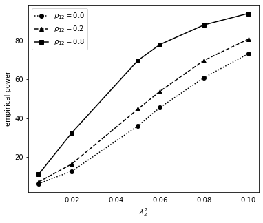
(a) Model $m_{1}$

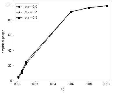
(b) Model $m_{2}$

Figure 1: Empirical power of the test that one variance is null in a linear model with (a) two random effects and (b) three random effects, for varying value of the tested variance and of the correlation coefficient.

We then study the effect of shrinkage on the type I error using model $m_{3}$. Results are presented in figure 2 for a theoretical level of 5%. We see that the procedure is sensitive to extreme values of $c_{N}$. The performances of the shrinked bootstrap procedure are stable as the number of nuisance parameters increases, provided that the shrinkage parameter $c_{N}$ is carefully chosen, whereas the performances of the regular bootstrap procedure with no shrinkage are downgraded in this context. Indeed choosing a value of $c_{N}\approx 0.24$, i.e. that shrinks most of the nuisance parameters, provides good results while choosing $c_{N}=0.9$, i.e. of the same order of magnitude as the non-zero variances of the model (here, $\lambda=1$) deteriorates the results. On the other hand, neglecting the nuisance parameters, which corresponds to the case $c_{N}=0$, also as an influence on the results and leads to an empirical level which is smaller than the theoretical one. These results suggest that in practice, users should be cautious when choosing the shrinkage parameter, and that smaller values of $c_{N}$ could be preferred over too large values since the impact on the type I error seems higher in the latter case.

Figure 2: Comparison of the parametric bootstrap procedure and the shrinked parametric bootstrap procedure in $m_{3}$, using $K=2500$ datasets of size $N=30$ and $B=300$ bootstrap replicates for varying numbers of nuisance parameters, and different shrinkage parameters $c_{N}$.

Level $\alpha$	boot	asym	max sd
1%	0.80	0.80	0.28
5%	5.10	3.60	0.70
10%	10.30	7.00	0.96

Table 3: Comparison of the bootsrap procedure and the asymptotic procedure in the test in $m_{4}$, using $K=1000$ datasets of size $N=40$ and $B=300$ bootstrap replicates.

boot., parametric bootstrap procedure; asym., asymptotic procedure; sd, standard deviation.

4.2 Real data application

We then apply our procedure to a study of white-browed coucal growth rates, available as a Dryad package [21]. We use the logistic growth model defined in (9) to describe the evolution of the body mass of the nestlings as a function of their age. More precisely, if we denote by $y_{ij}$ the body mass of nestling $i$ at age $t_{j}$ for $i=1,...,292$, $j=1,...,N_{i}$, we have that $\beta_{1}+\lambda_{1}\xi_{i1}$ is the asymptotic nestling body mass, $\beta_{2}+\lambda_{2}\xi_{i2}$ is the age (in days) at which nestling $i$ reaches half its asymptotic body mass and $\beta_{3}+\lambda_{3}\xi_{i3}$ is the growth rate of nestling $i$. When fitting the complete model the estimated scaling matrix is $\hat{\Lambda}=\textnormal{diag}(\sqrt{2}12.34,\sqrt{0}.89,\sqrt{0}.02)$, which motivates the test that $\lambda_{2}$ and $\lambda_{3}$ are null.

In order to test for the presence of randomness in the inflexion point and in the growth rate, we proceed sequentially. First, we test if the variances of both the inflexion point and the growth rate are null, i.e. we consider the test $T_{1}:H_{0}:\lambda_{2}=0,\lambda_{3}=0$ against $H_{1}:\lambda_{2}\geq 0,\lambda_{3}\geq 0$. If the null hypothesis in $T_{1}$ is rejected, we perform two univariate tests, one for each variance tested in $T_{1}$. More precisely, we consider the tests $T_{2}:H_{0}:\lambda_{3}=0$ against $H_{1}:\lambda_{3}\geq 0$ and $T_{3}:H_{0}:\lambda_{2}=0$ against $H_{1}:\lambda_{2}\geq 0$. If the null hypothesis is rejected in $T_{1}$, it means that at least one of the two tested variances is nonzero, thus we can then consider the univariate tests $T_{2}$ and $T_{3}$, where $\lambda_{2}$ and $\lambda_{3}$ might be nuisance parameters. For each test, we consider two procedures, one where the estimate of the potential nuisance parameter ($\lambda_{2}$ in $T_{2}$ and $\lambda_{3}$ in $T_{3}$) is shrinked toward zero, and another one without shrinkage. This choice enables to consider the two possible cases : $\lambda_{2}>c_{N}$ and $\lambda_{2}<c_{N}$ for $T_{2}$ and $\lambda_{3}>c_{N}$ and $\lambda_{3}<c_{N}$ for $T_{3}$. In practice the practitioner can choose the threshold according to his own level of significance of variability desired. For instance by saying that under X% of relative variability of a parameter, we consider it as a fixed effect. Table 4 compiles the results of the three tests.

Test	T1	T2		T3
lrt	$302.5$	1.6		278.2
procedure	no shrink	shrink	no shrink	shrink	no shrink
$p$–value	0	8.9	7.9	0	0

Table 4: Comparison of the $p$–value (in %) among the three tests $T1$, $T2$ and $T3$, using $B=1000$ bootstrap replicates..

shrink., shrinked parametric bootstrap procedure; no shrink., regular parametric bootstrap procedure without shrinkage

We can see that the procedures lead to different $p$-values, and can thus, in practice, lead to different conclusions with respect to the null hypothesis depending on the type I error considered.

5 Discussion

This work can lead to several future developments, both from a theoretical and a practical point of view. For example, the choice of the shrinking parameter $c_{N}$ is of interest for practitioners that would want to apply our procedure. This issue can be tackled from two perspectives. From an expert-based point of view, $c_{N}$ could be defined as a threshold, under which the variability of a random effect is not relevant in the task of interest. From a methodological point of view, it would be interesting to propose an automated procedure, following for example the idea of [6]. Our algorithm can be used indifferently for linear and nonlinear mixed effects models, however the computation time can be prohibitive in the latter case, especially for complex models. It would be interesting to find a criterion to optimize the choice of the bootstrap sample size. Another issue when dealing with complex models is the computation of the likelihood ratio test statistic. Indeed, it involves a ratio of likelihoods which are usually estimated separately using Monte Carlo approaches, leading to a biased estimate. This point is crucial since this quantity is calculated at each iteration of the bootstrap procedure.

6 Acknowledgment

This work was funded by the Stat4Plant project ANR-20-CE45-0012.

7 Supplementary material

We recall that we consider the following nonlinear mixed effects model, for any $i=1,...,N$ and any $j=1,..,J_{i}$:

$$\left\{\begin{array}[]{ll}y_{ij}&=g(x_{ij},\beta,\Lambda\xi_{i})+\varepsilon_{ij}\quad\varepsilon_{ij}\sim\mathcal{N}(0,\sigma^{2})\\ \xi_{i}&\sim\mathcal{N}\left(0,I_{p}\right)\\ \end{array}\right.$$ (10)

We also recall that the log–likelihood of the model given the data $y_{1:N}$ writes:

$$l(\theta;y_{1:N})=\log\{L_{\theta}(y_{1:N})\}=\log\{\prod_{i=1}^{N}f_{i}(y_{i};\theta)\}=\sum_{i=1}^{N}\log\{\int f_{i}(y_{i};\xi_{i},\theta)\pi(\xi_{i})d\xi_{i}\}.$$ (11)

Finally we write

$$\hat{\theta}_{N}=\arg\underset{\theta\in\Theta}{\sup}\quad l(\theta;y_{1:N}).$$ (12)

7.1 Different parametrizations for mixed effects models

The commonly used parametrization for nonlinear mixed effects models ([32] page 306) is for $i=1,...,N$, $j=1,...,J_{i}$ :

$$\left\{\begin{array}[]{ll}y_{ij}&=g(v_{ij},\phi_{i})+\varepsilon_{ij}\quad\varepsilon_{ij}\sim\mathcal{N}(0,\sigma^{2})\\ \phi_{i}&=A_{ij}\beta+B_{ij}b_{i}\quad b_{i}\sim\mathcal{N}\left(0,\Gamma\right)\\ \end{array}\right.$$ (13)

where $v_{ij}$, $A_{ij}$ and $B_{ij}$ are known covariates. With this definition, the log–likelihood is defined as follows :

$$l(\theta;y_{1:N})=\log\{L_{\theta}(y_{1:N})\}=\log\{\prod_{i=1}^{N}f_{i}(y_{i};\theta)\}=\sum_{i=1}^{N}\log\{\int f_{i}(y_{i};b_{i},\theta)\pi(b_{i};0,\Gamma)db_{i}\},$$ (14)

where $f_{i}(y_{i};b_{i},\theta)$ is the density of the conditional distribution of $y_{i}$ given $b_{i}$, and $\pi(b_{i};0,\Gamma)$ is the density of the $p$-dimensional centered Gaussian distribution with covariance $\Gamma$.

The change of variable $b_{i}=\Lambda\xi_{i}$ is a $\mathcal{C}^{1}$ diffeomorphism if and only if the diagonal coefficients of $\Lambda$ are strictly nonnegative. Therefore in our setting where this condition is not verified these two parametrizations are not equivalent.

In particular taking $\Lambda=0$ in (2) is equivalent to considering a fixed-effects nonlinear model, while in (14), taking $\Gamma\rightarrow 0$ makes $l(\theta;y_{1:N})\rightarrow-\infty$.

7.2 Proof of proposition 1

To prove the proposition we only have to prove that if the $m$th column of $\Lambda$ is $0$, then the odds orders of the partial derivatives of the log-likelihood with respect to the elements of this column are null regardless of the values of the $y_{1:N}$. We have, for all $n=1,..,p$:

$$\frac{\partial f_{i}(y_{i};\theta)}{\partial[\Lambda]_{nm}}|_{\theta=\theta_{0}}=\int_{\xi_{1}}\cdot\cdot\cdot\int_{\xi_{p}}\frac{\partial f_{i}(y_{i};\xi,\theta_{0})}{\partial[\Lambda]_{nm}}\pi(\xi_{1})d\xi_{1}...\pi(\xi_{p})d\xi_{p}$$

Given the definition of model 1 :

$$f_{i}(y_{i};\xi,\theta)=(2\pi\sigma^{2})^{-\frac{J_{i}}{2}}\\ exp\left[-\frac{\sum_{j=1}^{J_{i}}\left\{y_{ij}-g(x_{ij},\beta,\Lambda\xi)\right\}^{2}}{2\sigma^{2}}\right]$$

therefore,

$$\frac{\partial f_{i}(y_{i};\xi,\theta)}{\partial[\Lambda]_{nm}} \propto\frac{\partial\Lambda\xi}{\partial[\Lambda]_{mn}}\nabla_{\Lambda\xi}\exp\left[-\frac{\sum_{j=1}^{J_{i}}\left\{y_{ij}-g(x_{ij},\beta,\Lambda\xi)\right\}^{2}}{2\sigma^{2}}\right]$$

$$\propto\xi_{m}\nabla_{\Lambda\xi}\exp\left[-\frac{\sum_{j=1}^{J_{i}}\left\{y_{ij}-g(x_{ij},\beta,\Lambda\xi)\right\}^{2}}{2\sigma^{2}}\right]$$

Evaluated at $\theta=\theta_{0}$ the last term (the gradient) no longer depends on $\xi_{m}$ as the $m$th column of $\Lambda$ is null.

$$\frac{\partial f_{i}(y_{i};\theta)}{\partial[\Lambda]_{nm}}|_{\theta=\theta_{0}}\propto \int_{\xi_{m}}\xi_{m}\pi(\xi_{m})d\xi_{m}$$

$$\times\int\nabla_{\Lambda\xi}\exp\left[-\frac{\sum_{j=1}^{J_{i}}\left\{y_{ij}-g(x_{ij},\beta,\Lambda\xi)\right\}^{2}}{\sigma^{2}}\right]\mid_{\theta=\theta_{0}}\prod_{l\neq m}\pi(\xi_{l})d\xi_{l}$$

which is equal to $0$ as the first term of the right hand side equation is expectation of a standard gaussian distribution. We can apply the same reasoning to every odds order derivatives.

7.3 Proof of proposition 2

Due to assumption (1) we have that :

$$\underset{\theta\in\Theta}{\sup}\mathrm{E}\left\{l(\theta;y_{1})\right\}<\mathrm{E}\left\{l(\theta_{0};y_{1})\right\}$$ (15)

which comes from the identifiability of the model and the positivity of the Kullback-Leibler divergence. Assumption (2)$i)$ enables to apply the uniform law of large number to the log–likelihood. Then the result follows from arguments as in [1] lemma A.1.

7.4 Proof of proposition 4

To prove the consistency of the bootstrap maximum likelihood estimator, we will use the same reasoning, as in the proof of proposition 2. The sketch of the proof is similar to the one of [11].

We first want to show that :

$$\underset{\theta\in\Theta}{\sup}|\frac{1}{N}l(\theta;y^{*}_{1:N})-\mathrm{E}\left\{l(\theta;y_{1})\right\}|=o_{p^{*}}(1)$$

First of all we have that :

$$\underset{\theta\in\Theta}{\sup}|\frac{1}{N}l(\theta;y^{*}_{1:N})-\mathrm{E}\left\{l(\theta;y_{1})\right\}| \leq\underset{\theta\in\Theta}{\sup}A_{N}^{*}(\theta)+\underset{\theta\in\Theta}{\sup}A_{N}(\theta)$$

where :

$$A_{N}^{*}(\theta) =|\frac{1}{N}l(\theta;y^{*}_{1:N})-\mathrm{E}^{*}\left\{l(\theta;y_{1}^{*})\right\}|$$

$$A_{N}(\theta) =|\mathrm{E}^{*}\left\{l(\theta;y_{1}^{*})\right\}-\mathrm{E}\left\{l(\theta;y_{1})\right\}|$$

We now want to apply the uniform law of large numbers to $A_{N}(\theta)$, and it’s bootstrap version to $A_{N}^{*}(\theta)$. Therefore we shall show that both term converges toward $0$ and that they are lipshitz.
We first consider $A_{N}(\theta)$ for a given $\theta\in\Theta$.

$$\mathrm{E}^{*}\left\{l(\theta;y_{1}^{*})\right\} =\mathrm{E}\{l(\theta;y_{1}^{*})|y_{1:N}\}$$

$$=\int l(\theta;y_{1})f(y_{1};{\theta_{N}^{*}})dy_{1}$$

Using assumption (1), we can state that there exist $\theta^{+}$ between $\theta_{0}$ and ${\theta_{N}^{*}}$ such that,

$$|f(y_{1};{\theta_{N}^{*}})-f(y_{1};\theta_{0})| \leq\|\theta_{0}-{\theta_{N}^{*}}\|\|\nabla_{\theta}f(y_{1};\theta^{+})\|$$

$$\leq\|\theta_{0}-{\theta_{N}^{*}}\|\|\nabla_{\theta}\log\{f(y_{1};\theta^{+})\}\|f(y_{1};\theta^{+})$$

therefore,

$$A_{N}(\theta) \leq\int|l(\theta;y_{1})|||f(y_{1};{\theta_{N}^{*}})-f(y_{1};\theta_{0})|dy_{1}$$

$$\leq\int|l(\theta;y_{1})|\|\theta_{0}-{\theta_{N}^{*}}\|\|\nabla_{\theta}\log\{f(y_{1};\theta^{+})\}\|f(y_{1};\theta^{+})dy_{1}$$

$$\leq\|\theta_{0}-{\theta_{N}^{*}}\|\int|l(\theta;y_{1})|\|\nabla_{\theta}l(\theta^{+};y_{1})\}\|f(y_{1};\theta^{+})dy_{1}$$

Due to assumption (2)$i)$–$ii)$, $|l(\theta;y_{1})|\|\nabla_{\theta}l(\theta^{+};y_{1})\}\|$ is integrable with respect to the density $f(y_{1};\theta^{+})$. And finally using the elementary inequality ,

$$\frac{1}{2}(a^{2}+b^{2})\geq|ab|,\quad\forall a,b\in\mathbb{R}$$ (16)

we can state that

$$A_{N}(\theta) \leq\frac{1}{2}\|\theta_{0}-{\theta_{N}^{*}}\|\underset{\theta^{+}\in\Theta}{\sup}\int\underset{\Theta\in\Theta}{\sup}|l(\Theta;y_{1})|^{2}+\underset{\theta_{2}\in\Theta}{\sup}\|\nabla_{\theta}l(\theta_{2};y_{1})\}\|^{2}f(y_{1};\theta^{+})dy_{1}$$

Finally thanks to assumption (2), as $N\rightarrow+\infty$, it holds in probability that :

$$A_{N}(\theta)\rightarrow 0$$

We now consider :

$$A_{N}^{*}(\theta)=|\frac{1}{N}\sum_{i=1}^{N}l(\theta;y_{i}^{*})-\mathrm{E}^{*}\left\{l(\theta;y_{1}^{*})\right\}|$$

This quantity is a sum of conditionally independent and centered random variables. We can’t directly apply a law of large number as the parameter ${\theta_{N}^{*}}$ and the index of the sum depends both on $N$.

For every real nonnegative number $t$, it holds almost surely that :

$$\textnormal{pr}^{*}(A_{N}^{*}>t)\leq\textnormal{pr}^{*}\{\frac{1}{N}\sum_{i}|l(y_{i}^{*};\theta)-\mathrm{E}^{*}\left\{l(\theta;y_{1}^{*})\right\}|>t\}\leq\frac{\underset{\theta^{\prime}\in\Theta}{\sup}\mathrm{E}_{\theta^{\prime}}\{\underset{\theta\in\Theta}{\sup}|l(\theta;y_{1})|^{2}\}}{Nt^{2}}$$

by applying first triangular inequality and then Chebychev inequality, using assumption (2)$i)$. And finally $A_{N}^{*}(\theta)\rightarrow 0$ in probability, as $N\rightarrow+\infty$, which concludes the pointwise convergence. And we note that this result holds uniformly over $\Theta$ so:

$$\underset{\theta\in\Theta}{\sup}|\frac{1}{N}l(\theta;y^{*}_{1:N})-\mathrm{E}\left\{l(\theta;y_{1})\right\}|=o_{p^{*}}(1)$$

Let now use this result to show that the bootstrap maximum likelihood estimator is consistent.

Let $\varepsilon>0$, using equation (15), there exists $\delta>0$ such that:

$$\underset{\|\theta-\theta_{0}\|>\varepsilon}{\inf}\mathrm{E}\{l(\theta_{0};y_{1}))-\mathrm{E}(l(\theta;y_{1})\}\geq\delta$$

Let us introduce $\theta_{mle}^{B}=\arg\underset{\theta\in\Theta}{\max}\quad l(\theta;y_{1:N}^{*})$.

By writing $V_{\varepsilon}=\{\theta\in\Theta:\|\theta-\theta_{0}\|>\varepsilon\}$, we have that :

$$\textnormal{pr}^{*}(\theta_{mle}^{B}\in V_{\varepsilon}) \leq\textnormal{pr}^{*}\left[\mathrm{E}\{l(\theta_{0};y_{1})\}-\mathrm{E}\{l(\theta_{mle}^{B};y_{1}^{*})\}\geq\delta\right]$$

$$=\textnormal{pr}^{*}\left[\mathrm{E}\left\{l(\theta_{0};y_{1})\right\}-\frac{1}{N}l(\theta_{mle}^{B};y_{1:N}^{*})+\frac{1}{N}l(\theta_{mle}^{B};y_{1:N}^{*})-\mathrm{E}\left\{l(\theta_{mle}^{B};y_{1}^{*})\right\}\geq\delta\right]$$

$$\leq\textnormal{pr}^{*}\left[\mathrm{E}\{l(\theta_{0};y_{1})\}-\frac{1}{N}l(\theta_{0};y^{*}_{1:N})+\frac{1}{N}l(\theta_{mle}^{B};y_{1:N}^{*})-\mathrm{E}\{l(\theta_{mle}^{B};y_{1}^{*})\}\geq\delta\right]$$

$$\leq\textnormal{pr}^{*}\left\{2\underset{\theta\in\Theta}{\sup}|\frac{1}{N}l(\theta;y^{*}_{1:N})-\mathrm{E}\left\{l(\theta;y_{1})\right\}|\geq\delta\right\}$$

$$\leq o_{p}(1)$$

Which concludes the proof that $\theta_{mle}^{B}=\theta_{0}+o_{p^{*}}(1)$. The exact same proof still holds for the restricted bootstrap maximum likelihood estimator by replacing $\Theta$ by $\Theta_{0}$.

7.5 Quadratic approximation of the log–likelihood

To derive the asymptotic distribution of $LRT_{N}$, we expand the log-likelihood around $\theta_{0}$ (see [2] theorem 6). Under assumption (1), following the lines of [25], we can write:

$$l(\theta;y_{1:N})- l(\theta_{0};y_{1:N})=(\psi-\psi_{0})^{T}\nabla_{\psi}l(\theta_{0};y_{1:N})+\frac{1}{2}(\psi-\psi_{0})^{T}\nabla_{\psi}^{2}l(\theta_{0};y_{1:N})(\psi-\psi_{0})$$

$$+(1/2)\sum_{i,j=1,...,d_{\delta}}\delta_{i}\delta_{j}\frac{\partial^{2}l(\theta_{0};y_{1:N})}{\partial\delta_{i}\partial\delta_{j}}+(3/3!)(\psi-\psi_{0})^{T}\sum_{i,j=1,...,d_{\delta}}\delta_{i}\delta_{j}\frac{\partial^{3}l(\theta_{0};y_{1:N})}{\partial\delta_{i}\partial\delta_{j}\partial\psi}$$

$$+(1/2)\sum_{i,j=1,...,d_{\lambda}}\lambda_{i}\lambda_{j}\frac{\partial^{2}l(\theta_{0};y_{1:N})}{\partial\lambda_{i}\partial\lambda_{j}}+(3/3!)(\psi-\psi_{0})^{T}\sum_{i,j=1,...,d_{\lambda}}\lambda_{i}\lambda_{j}\frac{\partial^{3}l(\theta_{0};y_{1:N})}{\partial\lambda_{i}\partial\lambda_{j}\partial\psi}$$

$$+(6/4!)\sum_{i,j=1,...,d_{\delta}}\sum_{k,l=1,...,d_{\lambda}}\delta_{i}\delta_{j}\lambda_{k}\lambda_{l}\frac{\partial^{4}l(\theta_{0};y_{1:N})}{\partial\delta_{i}\partial\delta_{j}\partial\lambda_{k}\partial\lambda_{l}}$$

$$+(1/4!)\sum_{i,j,k,l=1,...,d_{\delta}}\delta_{i}\delta_{j}\delta_{k}\delta_{l}\frac{\partial^{4}l(\theta_{0};y_{1:N})}{\partial\delta_{i}\partial\delta_{j}\partial\delta_{k}\partial\delta_{l}}$$

$$+(1/4!)\sum_{i,j,k,l=1,...,d_{\lambda}}\lambda_{i}\lambda_{j}\lambda_{k}\lambda_{l}\frac{\partial^{4}l(\theta_{0};y_{1:N})}{\partial\lambda_{i}\partial\lambda_{j}\partial\lambda_{k}\partial\lambda_{l}}+R_{N}(\theta)$$

With $R_{N}(\theta)$ being the rest in the Taylor expansion . We define for all integers $i,j$ $c_{ij}=\frac{1}{2}$ if $i=j$ and $1$ otherwise. We also define $\mathcal{I}_{\lambda}=\{11,22,..,d_{\lambda}-1,d_{\lambda}\}$ and $\mathcal{I}_{\delta}=\{11,22,..,d_{\delta}-1,d_{\delta}\}$ that respectively index $v(\lambda)=(\lambda_{i}\lambda_{j})_{ij\in\mathcal{I}_{\lambda}}$ and $v(\delta)=(\delta_{i}\delta_{j})_{ij\in\mathcal{I}_{\delta}}$. For $ij\in\mathcal{I}_{\lambda}$ (respectively $\mathcal{I}_{\delta}$), we write $\frac{\partial^{2}l(\theta;y_{1:N})}{\partial v(\lambda)_{ij}}=\frac{\partial^{2}l(\theta;y_{1:N})}{\partial\lambda_{i}\lambda_{j}}$ (the same with $\delta$). With these notations we have that:

$$l(\theta;y_{1:N})-l(\theta_{0};y_{1:N})= (\psi-\psi_{0})^{T}\nabla_{\psi}l(\theta_{0};y_{1:N})+\frac{1}{2}(\psi-\psi_{0})^{T}\nabla_{\psi}^{2}l(\theta_{0};y_{1:N})(\psi-\psi_{0})$$

$$+\sum_{i\in\mathcal{I}_{\lambda}}v(\lambda)_{i}c_{i}\frac{\partial^{2}l(\theta;y_{1:N})}{\partial v(\lambda)_{i}}+(1/3)(\psi-\psi_{0})^{T}\sum_{i\in\mathcal{I}_{\lambda}}v(\lambda)_{i}c_{i}\frac{\partial^{3}l(\theta_{0};y_{1:N})}{\partial v(\lambda)_{i}\partial\psi}$$

$$+\sum_{i\in\mathcal{I}_{\delta}}v(\delta)_{i}c_{i}\frac{\partial^{2}l(\theta;y_{1:N})}{\partial v(\delta)_{i}}+(1/3)(\psi-\psi_{0})^{T}\sum_{i\in\mathcal{I}_{\delta}}v(\delta)_{i}c_{i}\frac{\partial^{3}l(\theta_{0};y_{1:N})}{\partial v(\delta)_{i}\partial\psi}$$

$$+4\times(6/4!)\sum_{i\in\mathcal{I}_{\lambda},j\in\mathcal{I}_{\delta}}c_{i}c_{j}v(\lambda)_{i}v(\delta)_{j}\frac{\partial^{4}l(\theta_{0};y_{1:N})}{\partial v(\lambda)_{i}\partial v(\delta)_{j}}$$

$$+(4/4!)\sum_{i\in\mathcal{I}_{\delta},j\in\mathcal{I}_{\delta}}c_{i}c_{j}v(\delta)_{i}v(\delta)_{j}\frac{\partial^{4}l(\theta_{0};y_{1:N})}{\partial v(\delta)_{i}\partial v(\delta)_{j}}$$

$$+(4/4!)\sum_{i\in\mathcal{I}_{\lambda},j\in\mathcal{I}_{\lambda}}c_{i}c_{j}v(\lambda)_{i}v(\lambda)_{j}\frac{\partial^{4}l(\theta_{0};y_{1:N})}{\partial v(\lambda)_{i}\partial v(\lambda)_{j}}+R_{N}(\theta)$$

We define the reparametrization of $\theta$ : $\phi(\theta)=(\psi,v(\delta),v(\lambda))$.

By writing $\tilde{\nabla}_{v(\lambda)}l(\theta;y_{1:N})=\left(c_{i}\frac{\partial^{2}l(\theta;y_{1:N})}{\partial v(\lambda)_{i}}\right)_{i\in\mathcal{I_{\lambda}}}$ (similarly for $\tilde{\nabla}_{v(\delta)}l(\theta;y_{1:N})$) and $\tilde{\nabla}^{2}_{v(\lambda)}l(\theta;y_{1:N})=(c_{i}c_{j}\frac{\partial^{4}l(\theta;y_{1:N})}{\partial v(\lambda)_{i}\partial v(\lambda)_{j}})_{i,j=1,...,d_{\lambda}}$ (similarly for $\tilde{\nabla}^{2}_{v(\delta)}l(\theta;y_{1:N})$ ), we also define :

$$\tilde{S}_{N}(\theta_{0})=\sqrt{N}^{-1}\left(\begin{tabular}[]{ll}$\nabla_{\psi}l(\theta_{0};y_{1:N})^{T}$, $\tilde{\nabla}_{v(\delta)}l(\theta_{0};y_{1:N})^{T}$, $\tilde{\nabla}_{v(\lambda)}l(\theta_{0};y_{1:N})^{T}$\end{tabular}\right)^{T}$$

$$\tilde{I}_{N}(\theta_{0})=\begin{pmatrix}I_{N,\psi}(\theta_{0})&I_{N,\psi,v(\delta)}(\theta_{0})&I_{N,\psi,v(\lambda)}(\theta_{0})\\ I_{N,\psi,v(\delta)}(\theta_{0})^{T}&I_{N,v(\delta)}(\theta_{0})&I_{N,v(\delta),v(\lambda)}(\theta_{0})\\ I_{N,\psi,v(\lambda)}(\theta_{0})^{T}&I_{N,v(\delta),v(\lambda)}(\theta_{0})^{T}&I_{N,v(\lambda)}(\theta_{0})\end{pmatrix}$$

Where $I_{N,\psi}(\theta_{0})=-\frac{1}{N}\nabla^{2}_{\psi}l(\theta_{0};y_{1:N})$, $I_{N,\psi,v(\lambda)}(\theta_{0})=\left(-\frac{c_{i}}{3N}\frac{\partial^{3}l(\theta_{0};y_{1:N})}{\partial\psi\partial v(\lambda)_{i}}\right)_{.,i\in\mathcal{I}_{\lambda}}$, $I_{N,\psi,v(\delta)}(\theta_{0})=\left(-\frac{c_{i}}{3N}\frac{\partial^{3}l(\theta_{0};y_{1:N})}{\partial\psi\partial v(\delta)_{i}}\right)_{.,i\in\mathcal{I}_{\delta}}$, $I_{N,v(\lambda)}(\theta_{0})=-\frac{1}{3N}\tilde{\nabla}^{2}_{v(\lambda)}l(\theta_{0};y_{1:N})$, $I_{N,v(\delta)}(\theta_{0})=-\frac{1}{3N}\tilde{\nabla}^{2}_{v(\delta)}l(\theta_{0};y_{1:N})$, $I_{N,v(\lambda),v(\delta)}(\theta_{0})=(-\frac{1}{N}c_{i}c_{j}\frac{\partial^{4}l(\theta_{0};y_{1:N})}{\partial v(\lambda)_{i}\partial v(\delta)_{j}})_{i\in\mathcal{I}_{\lambda},j\in\mathcal{I}_{\delta}}$.

Where the notation $(a_{i})_{.,i\in\mathcal{I}}$ stands for a $dim(a_{i})\times card(\mathcal{I})$ matrix whose columns are $a_{i}$ for $i\in\mathcal{I}$.

With these new notations we obtain the following quadratic approximation of the log–likelihood :

$$\begin{split}l(\theta;y_{1:N})-l(\theta_{0};y_{1:N})=\sqrt{N}(&\phi(\theta)-\phi(\theta_{0}))^{T}\tilde{S}_{N}(\theta_{0})\\ &-\frac{1}{2}\sqrt{N}(\phi(\theta)-\phi(\theta_{0}))^{T}\tilde{I}_{N}(\theta_{0})\sqrt{N}(\phi(\theta)-\phi(\theta_{0}))+R_{N}(\theta)\end{split}$$ (17)

7.6 Asymptotic distribution of the likelihood ratio test statistic

We start from the expansion of the log–likelihood (17) derived in the last section, that we rewrite:

$$\begin{split}l(\theta;y_{1:N})-l(\theta_{0};y_{1:N})=\frac{1}{2}&Z_{N}(\theta_{0})^{T}\tilde{I}_{N}(\theta_{0})Z_{N}(\theta_{0})\\ &-\frac{1}{2}\left(t_{N}(\theta)-Z_{N}(\theta_{0})\right)^{T}\tilde{I}_{N}(\theta_{0})\left(t_{N}(\theta)-Z_{N}(\theta_{0})\right)+R_{N}(\theta)\end{split}$$

where $t_{N}(\theta)=\sqrt{N}(\phi(\theta)-\phi(\theta_{0}))$ and $Z_{N}(\theta_{0})=\tilde{I}_{N}(\theta_{0})^{-1}\tilde{S}_{N}(\theta_{0})$

Remark 8

We consider the quantity $\tilde{I}_{N}(\theta_{0})^{-1}$ which implies that $\tilde{I}_{N}(\theta_{0})$ is non-singular which may not be always true. However under assumption (3), the probability that $\tilde{I}_{N}(\theta_{0})$ is non-singular tends to 1 as $N\rightarrow+\infty$. _□

The set a feasible values for $t_{N}(\theta)$ is:

$$t_{N}(\Theta)=\{\sqrt{N}\left(\Theta_{\psi}-\psi_{0}\right)\}\times\{\sqrt{N}\left(v(\Theta_{\lambda})-v(\lambda_{0})\right)\}\times\{\left(v(\Theta_{\delta})-v(\delta_{0})\right)\}$$ (18)

$t_{N}(\Theta)$ does not depend on $N$ ( it is a cartesian product whose terms are whether $\mathbb{R}$ or $[0,+\infty[$), and it is locally approximated by a cone (in fact it is a cone), we write it $\mathcal{C}(\Theta)$. Therefore if we prove that $R_{N}(\theta)$ is $o_{p}(1)$ when evaluated at the maximum likelihood estimator, we can apply the result from [2]. For more details see [2] and paragraph 4.3.

In order to apply the theory of Andrews, one shall prove that $\tilde{I}_{N}(\theta_{0})$ converges in probability toward a nonnegative matrix $\tilde{I}(\theta_{0})$, and that $\tilde{S}_{N}(\theta_{0})$ converges weakly to a random variable $U(\theta_{0})$.

1) Let $d_{\tilde{I}}\in\mathbb{N}$ such that $\tilde{I}_{N}(\theta_{0})\in\mathbb{R}^{d_{\tilde{I}}\times d_{\tilde{I}}}$, let $1\leq m,n\leq d_{\tilde{I}}$. We can write:

$$\left[\tilde{I}_{N}(\theta_{0})\right]_{m,n}=\frac{1}{N}\sum_{i=1}^{N}h_{m,n}^{(i)}(\theta_{0})$$

where $h_{m,n}^{(i)}(\theta_{0})$ is of the form:

$$h_{m,n}^{(i)}(\theta_{0})=c_{m,n}\frac{\partial^{k}\log f(y_{i};\theta)}{\partial\theta_{i_{1}}...\partial\theta_{i_{k}}}|_{\theta=\theta_{0}}$$

with $c_{m,n}\in\mathbb{R}$, $k\in\{2,4\}$, $1\leq i_{1},...,i_{k}\leq d_{\lambda}+d_{\psi}+d_{\delta}$.

With assumption (2) we can apply the law of large numbers to this empirical mean and therefore it holds in probability that:

$$\tilde{I}_{N}(\theta_{0})\underset{N\rightarrow+\infty}{\longrightarrow}\left[\mathrm{E}\{h_{m,n}^{(1)}(\theta_{0})\}\right]_{1\leq m,n\leq q_{I}}=\tilde{I}(\theta_{0})$$

2) We now consider $\tilde{S}_{N}(\theta_{0})$.

First the score is centered,

$$\mathrm{E}\left[\nabla_{\psi}\log f(x_{i};\theta_{0})\right]=0$$

then, due to proposition (1), $\forall m,n=1,...,q_{\lambda}$,

$$\mathrm{E}\left[\frac{\partial^{2}\log f(y_{i};\theta_{0})}{\partial\lambda_{m}\partial\lambda_{n}}\right]=-\mathrm{E}\left[\frac{\partial\log f(y_{i};\theta_{0})}{\partial\lambda_{m}}\frac{\partial\log f(y_{i};\theta_{0})}{\partial\lambda_{n}}\right]=0$$

We apply the central limit theorem to $\tilde{S}_{N}(\theta_{0})$ which is a sum of independent and identically distributed centered random variables with finite variances, and therefore $\tilde{S}_{N}(\theta_{0})$ converges weakly to a random variable $U(\theta_{0})$

By doing the exact same quadratic approximation and development but considering the parameter space $\Theta_{0}$, combining (18)–(20), we use [2] to obtain :

$$LRT_{\infty}=\underset{t\in\mathcal{C}(\Theta_{0})}{\inf}\|t-\tilde{I}(\theta_{0})^{-1}U(\theta_{0})\|_{\tilde{I}(\theta_{0})}-\underset{t\in\mathcal{C}(\Theta)}{\inf}\|t-\tilde{I}(\theta_{0})^{-1}U(\theta_{0}))\|_{\tilde{I}(\theta_{0})}$$ (19)

Which leads to the expression of $LRT_{\infty}$.

7.7 Proof of proposition 3

To obtain an explicit form for $R_{N}(\theta)$ we use the multivariate version of Taylor-Lagrange formula, which is for instance defined in [2] Theorem 6.

This way we have that $R_{N}(\theta)$ is a sum of higher order derivatives with respect to $\psi$ and the fourth crossed derivatives with respect to $\lambda$. Given assumption (2) all the derivatives of the log-likelihood are $\mathcal{O}_{p}(N)$, using Cauchy-Schwartz inequality and the fact that $\|t_{N}(\theta)\|^{2}=N\left(\|\psi-\psi_{0}\|^{2}+\|v(\delta)\|^{2}+\|v(\lambda)\|^{2}\right)=N\left(\|\psi-\psi_{0}\|^{2}+\|\lambda\|^{4}+\|\delta\|^{4}\right)\mathcal{O}(1)$ we have that:

$$|R_{N}(\theta)|\leq\mathcal{O}_{p}(N)(\|\psi-\psi_{0}\|^{3} +\|\psi-\psi_{0}\|^{4}+\|\psi-\psi_{0}\|^{2}\|\lambda\|^{2}+\|\psi-\psi_{0}\|^{2}\|\delta\|^{2})$$

$$+\|\delta\|^{4}\left|\sum_{m,n,o,p=1,...,d_{\delta}}\frac{\partial^{4}l(\theta^{+};y_{1:N})}{\partial\delta_{m}\partial\delta_{n}\partial\delta_{o}\partial\delta_{p}}-\frac{\partial^{4}l(\theta_{0};y_{1:N})}{\partial\delta_{m}\partial\delta_{n}\partial\delta_{o}\partial\delta_{p}}\right|$$

$$+\|\lambda\|^{4}\left|\sum_{m,n,o,p=1,...,d_{\lambda}}\frac{\partial^{4}l(\theta^{+};y_{1:N})}{\partial\lambda_{m}\partial\lambda_{n}\partial\lambda_{o}\partial\lambda_{p}}-\frac{\partial^{4}l(\theta_{0};y_{1:N})}{\partial\lambda_{m}\partial\lambda_{n}\partial\lambda_{o}\partial\lambda_{p}}\right|$$

and then:

$$|R_{N}(\theta)|\leq\mathcal{O}_{p}(1)\|t_{N}(\theta)\|^{2}(o_{p}(1) +\frac{1}{N}\left|\sum_{m,n,o,p=1,...,d_{\lambda}}\frac{\partial^{4}l(\theta^{+};y_{1:N})}{\partial\lambda_{m}\partial\lambda_{n}\partial\lambda_{o}\partial\lambda_{p}}-\frac{\partial^{4}l(\theta_{0};y_{1:N})}{\partial\lambda_{m}\partial\lambda_{n}\partial\lambda_{o}\partial\lambda_{p}}\right|$$

$$+\frac{1}{N}\left|\sum_{m,n,o,p=1,...,d_{\delta}}\frac{\partial^{4}l(\theta^{+};y_{1:N})}{\partial\delta_{m}\partial\delta_{n}\partial\delta_{o}\partial\delta_{p}}-\frac{\partial^{4}l(\theta_{0};y_{1:N})}{\partial\delta_{m}\partial\delta_{n}\partial\delta_{o}\partial\delta_{p}}\right|)$$

where $\theta^{+}=\theta_{0}+t(\theta-\theta_{0})$ for some $0<t<1$.

To show that the last two terms tend to zero we proceed as follows :

$$\frac{1}{N}|\sum_{m,n,o,p=1,...,d_{\lambda}}\frac{\partial^{4}l(\theta^{+};y_{1:N})}{\partial\lambda_{m}\partial\lambda_{n}\partial\lambda_{o}\partial\lambda_{p}} -\frac{\partial^{4}l(\theta_{0};y_{1:N})}{\partial\lambda_{m}\partial\lambda_{n}\partial\lambda_{o}\partial\lambda_{p}}|=$$

$$\frac{1}{N}|\sum_{m,n,o,p=1,...,d_{\lambda}}\frac{\partial^{4}l(\theta^{+};y_{1:N})}{\partial\lambda_{m}\partial\lambda_{n}\partial\lambda_{o}\partial\lambda_{p}}-\mathrm{E}\left[\sum_{m,n,o,p=1,...,d_{\lambda}}\frac{\partial^{4}l(\theta^{+};y_{1})}{\partial\lambda_{m}\partial\lambda_{n}\partial\lambda_{o}\partial\lambda_{p}}\right]$$

$$+\mathrm{E}\left[\sum_{m,n,o,p=1,...,d_{\lambda}}\frac{\partial^{4}l(\theta^{+};y_{1:N})}{\partial\lambda_{m}\partial\lambda_{1}\partial\lambda_{o}\partial\lambda_{p}}\right]-\mathrm{E}\left[\frac{\partial^{4}l(\theta_{0};y_{1})}{\partial\lambda_{m}\partial\lambda_{n}\partial\lambda_{o}\partial\lambda_{p}}\right]$$

$$+\mathrm{E}\left[\frac{\partial^{4}l(\theta_{0};y_{1})}{\partial\lambda_{m}\partial\lambda_{n}\partial\lambda_{o}\partial\lambda_{p}}\right]-\frac{\partial^{4}l(\theta_{0};y_{1:N})}{\partial\lambda_{m}\partial\lambda_{n}\partial\lambda_{o}\partial\lambda_{p}}|$$

We then apply triangular inequality to separate the 3 terms. The first and third terms are empirical means of centered random variables with bounded variances (assumption (2)$v)$). Therefore we can use each time Chebychev’s inequality to obtain a weak law of large number and obtain the consistency toward $0$. For the second term,

$$|\sum_{m,n,o,p=1,...,d_{\lambda}}\frac{\partial^{4}l(\theta^{+};y_{1})}{\partial\lambda_{m}\partial\lambda_{1}\partial\lambda_{o}\partial\lambda_{p}}-\sum_{m,n,o,p=1,...,d_{\lambda}}\frac{\partial^{4}l(\theta;y_{1})}{\partial\lambda_{m}\partial\lambda_{1}\partial\lambda_{o}\partial\lambda_{p}}|\leq 2C\underset{\theta\in\Theta}{\sup}\|\nabla^{4}_{\theta}l(\theta;y_{1})\|$$

where $C$ is the nonnegative constant that appears in the equivalence between the L1 and L2 norm. When we evaluate at $\theta=\hat{\theta}_{N}$, $\theta^{+}=\theta_{0}+t(\hat{\theta}_{N}-\theta_{0})\rightarrow\theta_{0}$ in probability, as $N\rightarrow+\infty$. And by continuity of $\nabla^{4}_{\theta}l(\cdot;y_{1})$, and dominated convergence, the second term also converges toward $0$. Finally we obtain :

$$|R_{N}(\hat{\theta}_{N})|\leq o_{p}(1)\|t_{N}(\hat{\theta}_{N})\|^{2}$$

And then: $0\leq l(\hat{\theta}_{N};y_{1:N})-l(\theta_{0};y_{1:N})$
$\leq\|\tilde{S}_{N}(\theta_{0})\|\|t_{N}(\hat{\theta}_{N})\|-\frac{1}{2}\|t_{N}(\hat{\theta}_{N})\|^{2}_{\tilde{I}_{N}(\theta_{0})}+o_{p}(\|t_{N}(\hat{\theta}_{N})\|^{2})$
$\leq\|\tilde{S}_{N}(\theta_{0})\|\|t_{N}(\hat{\theta}_{N})\|-\frac{1}{2}(o_{p}(1)+a)\|t_{N}(\hat{\theta}_{N})\|^{2}$
where

$$a=\underset{N>n_{0}}{\inf}\underset{x\neq 0}{\inf}\frac{\|x\|^{2}_{\tilde{I}_{N}(\theta_{0})}}{\|x\|^{2}}$$

where $\|x\|_{A}$ stands for $x^{T}Ax$, with $A$ being a positive definite symmetric matrix.

By taking $n_{0}$ large enough so that for every $N>n_{0}$, $\tilde{I}_{N}(\theta_{0})\succ 0$ (assumption (3)) we have that $0<a<+\infty$. The last inequality, shows that for $N$ large enough, this polynomial of degree 2 in $\|t_{N}(\hat{\theta}_{N})\|$ is upper bounded (dominant coefficient negative) and lower bounded by 0. Which shows that

$$t_{N}(\hat{\theta}_{N})=\mathcal{O}_{p}(1)$$

which concludes the proof, and :

$$R_{N}(\hat{\theta}_{N})=o_{p}(1)\mathcal{O}_{p}(1)=o_{p}(1)$$ (20)

which is fundamental for the proof of theorem (1)

7.8 Proof of theorem 1

Now that we derived the expression of $LRT_{\infty}$, it remains to show that the bootstrap statistic also converges weakly in probability to this random variable. To do so we first derive a bootstrap quadratic approximation as in (21), where the expansion is done around ${\theta_{N}^{*}}$, as it is the true parameter of the bootstrap data. We obtain that :

$$\begin{split}l(\theta;y^{*}_{1:N})-l({\theta_{N}^{*}};y_{1:N}^{*})=\frac{1}{2}&Z_{N}^{*}({\theta_{N}^{*}})^{T}\tilde{I}^{*}_{N}({\theta_{N}^{*}})Z_{N}^{*}({\theta_{N}^{*}})\\ &-\frac{1}{2}\left(t_{N}^{*}(\theta)-Z_{N}^{*}({\theta_{N}^{*}})\right)^{T}\tilde{I}^{*}_{N}({\theta_{N}^{*}})\left(t_{N}^{*}(\theta)-Z_{N}^{*}({\theta_{N}^{*}})\right)+R_{N}^{*}(\theta)\end{split}$$ (21)

where the exponent ^∗ stands for "evaluated on the bootstrap data". The following proof will follow three main steps.

First we show that the bootstrap version of $\tilde{I}_{N}(\theta_{0})$ and of $\tilde{S}_{N}(\theta_{0})$ have the correct conditional limiting distribution which means that :

$$\left\{\begin{tabular}[]{ll}$\tilde{I}_{N}^{*}({\theta_{N}^{*}})-\tilde{I}_{N}(\theta_{0})=o_{p^{*}}(1)$\\ $\forall t\in\mathds{R}^{d_{\tilde{I}}}\quad\textnormal{pr}^{*}\{\tilde{S}^{*}_{N}({\theta_{N}^{*}})<t\}-\textnormal{pr}\{\tilde{S}_{N}(\theta_{0})<t\}=o_{p}(1)$\end{tabular}\right.$$ (22)

Second, we show that the new terms in the quadratic approximation that are supposed to be null converge toward $0$ thanks to the shrinkage parameter.

Finally we show that the rest in the bootstrap quadratic approximation is a $o_{p^{*}}(1)$.

We first consider the case with no nuisance parameters i.e. $\theta=(\psi,\lambda)$ to lighten the notations and work in two steps.

We first consider $\tilde{I}_{N}({\theta_{N}^{*}})$. We write :

$$\left[\tilde{I}_{N}({\theta_{N}^{*}})\right]_{m,n}=\frac{1}{N}\sum_{i=1}^{N}h_{m,n}^{(i)*}({\theta_{N}^{*}})$$

where $h_{m,n}^{(i)}({\theta_{N}^{*}})$ is of the form:

$$h_{m,n}^{(i)*}({\theta_{N}^{*}})=c_{m,n}\frac{\partial^{k}\log f(y_{i};{\theta_{N}^{*}})}{\partial\theta_{i_{1}}...\partial\theta_{i_{k}}}$$

with $c_{m,n}\in\mathbb{R}$, $k\in\{2,4\}$, $1\leq i_{1},...,i_{k}\leq q_{\lambda}+q_{\psi}$.

We want to show that:

$$\frac{1}{N}\sum_{i=1}^{N}h_{m,n}^{(i)*}({\theta_{N}^{*}})-\mathrm{E}\{h_{m,n}^{(1)}(\theta_{0})\}=o_{p^{*}}(1)$$

To show that we decompose the difference:

$$\frac{1}{N}\sum_{i=1}^{N}h_{m,n}^{(i)*}({\theta_{N}^{*}})-\mathrm{E}\left[h_{m,n}^{(1)}(\theta_{0})\right]$$

as:

$$\overbrace{\frac{1}{N}\sum_{i=1}^{N}h_{m,n}^{(i)*}({\theta_{N}^{*}})-\mathrm{E}^{*}\left[h_{m,n}^{(1)*}({\theta_{N}^{*}})\right]}^{(T1)}+\overbrace{\mathrm{E}^{*}[h_{m,n}^{(1)*}({\theta_{N}^{*}})]-\mathrm{E}^{*}[h_{m,n}^{(1)*}(\theta_{0})]}^{(T2)}+\overbrace{\mathrm{E}^{*}[h_{m,n}^{(1)*}(\theta_{0})]-\mathrm{E}\left[h_{m,n}^{(1)}(\theta_{0})\right]}^{(T3)}$$

The term $(T1)$ is a sum of centered random variables, we can apply Chebychev’s inequality to have the convergence towards $0$ (using assumption (2) to have that the variance is $\mathcal{O}_{p}(1)$.

The term $(T2)$ is controlled as follows :

$$|\mathrm{E}^{*}[(h_{m,n}^{(1)*}({\theta_{N}^{*}})-h_{m,n}^{(1)*}(\theta_{0}))]| \leq\mathrm{E}^{*}\left[|(h_{m,n}^{(1)*}({\theta_{N}^{*}})-h_{m,n}^{(1)*}(\theta_{0}))|\right]$$

$$\leq\underset{\theta\in\Theta}{\sup}\mathrm{E}_{\theta}\left[|(h_{m,n}^{(1)*}({\theta_{N}^{*}})-h_{m,n}^{(1)*}(\theta_{0}))|\right]$$

as $|(h_{m,n}^{(1)*}({\theta_{N}^{*}})-h_{m,n}^{(1)*}(\theta_{0}))|\leq 2\underset{\theta\in\Theta}{\sup}|h_{m,n}^{(1)}(\theta)|$ almost surely, using assumption 2 and thanks to the consistency of ${\theta_{N}^{*}}$ we can use the dominated convergence theorem to prove the convergence in probability toward $0$.

Finally we deal with $(T3)$ as follows :

$$|\mathrm{E}^{*}[h_{m,n}^{(1)*}(\theta_{0})]-\mathrm{E}\left[h_{m,n}^{(1)}(\theta_{0})\right]| =|\int h_{m,n}^{(1)*}(\theta_{0})\{f(y;{\theta_{N}^{*}})-f(y;\theta_{0})\}dy|$$

$$\leq\int|h_{m,n}^{(1)*}(\theta_{0})||f(y;{\theta_{N}^{*}})-f(y;\theta_{0})|dy$$

To show that this term tends toward $0$ we use another time the equation (16), first we use a taylor expansion, there exist $\theta^{+}$ between $\theta_{0}$ and ${\theta_{N}^{*}}$ such that :

$$f(y;{\theta_{N}^{*}})-f(y;\theta_{0}) =({\theta_{N}^{*}}-\theta_{0})^{T}\nabla_{\theta}f(y;\theta^{+})$$

$$=({\theta_{N}^{*}}-\theta_{0})^{T}\nabla_{\theta}\log f(y;\theta^{+})f(y;\theta^{+})$$

therefore,

$$|f(y;{\theta_{N}^{*}})-f(y;\theta_{0})| \leq\|{\theta_{N}^{*}}-\theta_{0}\|\|\nabla_{\theta}\log f(y;\theta^{+})\|f(y;\theta^{+})$$

and,

$$|\mathrm{E}^{*}[h_{m,n}^{(1)*}(\theta_{0})]- \mathrm{E}\left[h_{m,n}^{(1)}(\theta_{0})\right]|\leq\|{\theta_{N}^{*}}-\theta_{0}\|\int|h_{m,n}^{(1)*}(\theta_{0})|\|\nabla_{\theta}\log f(y;\theta^{+})\|f(y;\theta^{+})dy$$

$$\leq\|{\theta_{N}^{*}}-\theta_{0}\|\int\frac{1}{2}\left\{|h_{m,n}^{(1)*}(\theta_{0})|^{2}+\|\nabla_{\theta}\log f(y;\theta^{+})\|^{2}\right\}f(y;\theta^{+})dy$$

Thanks to assumption (2), as ${\theta_{N}^{*}}-\theta_{0}=o_{p}(1)$ this last term is $o_{p}(1)$ as $N\rightarrow+\infty$.

We then consider $\tilde{S}_{N}^{*}({\theta_{N}^{*}})$, which is $\sqrt{N}$ times a sum of (conditionally) independent, centered, with finite variance random variables. Therefore, by proving that :

$$\mathrm{E}^{*}[\tilde{S}_{N}^{*}({\theta_{N}^{*}})\tilde{S}_{N}^{*}({\theta_{N}^{*}})^{T}]-\mathrm{E}\left[\tilde{S}_{1}(\theta_{0})^{T}\tilde{S}_{1}(\theta_{0})^{T}\right]=o_{p}(1)$$ (23)

and applying a multivariate version of the conditional central limit theorem of [10], it will conclude the second part of (13). Our third moment condition, and the consistency of the variance matrix of the score is much stronger then the Lindberg Feller conditions.

For each $m,n$, $\left[\tilde{S}_{N}^{*}({\theta_{N}^{*}})\tilde{S}_{N}^{*}({\theta_{N}^{*}})^{T}\right]_{m,n}$ can also be written as $\frac{1}{N}\sum_{i=1}^{N}h_{m,n}^{(i)*}({\theta_{N}^{*}})$, where $h_{m,n}^{(i)*}({\theta_{N}^{*}})=[\tilde{S}_{N}^{*}({\theta_{N}^{*}})]_{m}\times[\tilde{S}_{N}^{*}({\theta_{N}^{*}})]_{n}$ . Due to assumption (2)$ii)$–$iii)$, and the elementary equation (16), $\mathrm{E}\left[h_{m,n}^{(i)*}({\theta_{N}^{*}})^{3/2}\right]<+\infty$.

In order to prove (23), we once again split the sum :

$$\mathrm{E}^{*}[h_{m,n}^{(1)*}({\theta_{N}^{*}})]- \mathrm{E}\left[h_{m,n}^{(1)}(\theta_{0})\right]=$$

$$\overbrace{\mathrm{E}^{*}[h_{m,n}^{(1)*}({\theta_{N}^{*}})]-\mathrm{E}^{*}\left[h_{m,n}^{(1)*}(\theta_{0})\right]}^{(S1)} +\overbrace{\mathrm{E}^{*}[h_{m,n}^{(1)*}(\theta_{0})]-\mathrm{E}\left[h_{m,n}^{(1)}(\theta_{0})\right]}^{(S2)}$$

We first deal with $(S1)$ :

$$|\mathrm{E}^{*}[h_{m,n}^{(1)*}({\theta_{N}^{*}})]-\mathrm{E}^{*}\left[h_{m,n}^{(1)*}(\theta_{0})\right]| \leq\underset{\theta\in\Theta}{\sup}\quad|\mathrm{E}_{\theta}[h_{m,n}^{(1)*}({\theta_{N}^{*}})-h_{m,n}^{(1)*}(\theta_{0})]|$$

$$\leq\underset{\theta\in\Theta}{\sup}\quad\mathrm{E}_{\theta}[|h_{m,n}^{(1)*}({\theta_{N}^{*}})-h_{m,n}^{(1)*}(\theta_{0})|]$$

$$\leq 2\underset{\theta\in\Theta}{\sup}\quad\mathrm{E}_{\theta}[\underset{\theta^{\prime}\in\Theta}{\sup}|h_{m,n}^{(1)*}(\theta^{\prime})|]$$

$$<+\infty$$

Which enables, to apply dominated convergence to the first term, as $\hat{\theta}_{N}$ is consistent.

For $(S2)$ we proceed as follows :

$$|\mathrm{E}^{*}[h_{m,n}^{(1)*}(\theta_{0})]-\mathrm{E}\left[h_{m,n}^{(1)}(\theta_{0})\right]| =|\int h_{m,n}^{(1)*}(\theta_{0})\{f(y;{\theta_{N}^{*}})-f(y;\theta_{0})\}dy|$$

$$\leq\int|h_{m,n}^{(1)*}(\theta_{0})||f(y;{\theta_{N}^{*}})-f(y;\theta_{0})|dy$$

To show that this term tends toward $0$ we use the same reasonning as before, first we use a Taylor expansion: there exist $\theta^{+}$ between $\theta_{0}$ and ${\theta_{N}^{*}}$ such that :

$$f(y;{\theta_{N}^{*}})-f(y;\theta_{0}) =({\theta_{N}^{*}}-\theta_{0})^{T}\nabla_{\theta}f(y;\theta^{+})$$

$$=({\theta_{N}^{*}}-\theta_{0})^{T}\nabla_{\theta}\log f(y;\theta^{+})f(y;\theta^{+})$$

therefore,

$$|f(y;{\theta_{N}^{*}})-f(y;\theta_{0})| \leq\|{\theta_{N}^{*}}-\theta_{0}\|\|\nabla_{\theta}\log f(y;\theta^{+})\|f(y;\theta^{+})$$

and,

$$|\mathrm{E}^{*}[h_{m,n}^{(1)*}(\theta_{0})]- \mathrm{E}\left[h_{m,n}^{(1)}(\theta_{0})\right]|\leq\|{\theta_{N}^{*}}-\theta_{0}\|\int|h_{m,n}^{(1)*}(\theta_{0})|\|\nabla_{\theta}\log f(y;\theta^{+})\|f(y;\theta^{+})dy$$

We can’t directly use equation (16) here because $h_{m,n}^{(1)}(\theta)$ doesn’t admit second order moments ($\tilde{S}_{N}(\theta)$ admits third order moments). Thanks to Holder’s inequality using $p=\frac{3}{2}$ and $q=3$ we have that :

$$\|{\theta_{N}^{*}}-\theta_{0}\|\int|h_{m,n}^{(1)*}(\theta_{0})|\|\nabla_{\theta}\log f(y;\theta^{+})\|f(y;\theta^{+})dy$$

$$\leq\|{\theta_{N}^{*}}-\theta_{0}\|\left(\int\|\nabla_{\theta}\log f(y;\theta^{+})\|^{3}f(y;\theta^{+})dy\right)^{\frac{1}{3}}\left(\int|h_{m,n}^{(1)*}(\theta_{0})|^{\frac{3}{2}}f(y;\theta^{+})dy\right)^{\frac{2}{3}}$$

$$=o_{p}(1)$$

the last inequality holds thanks to assumption (2)$ii)$–$iii)$ that enables to state that the two integrals are finite. That concludes the proof that (23) holds.

We now deal with the nuisance parameters. The proof starts the same way as before. The issue is that the odd derivatives with respect to the parameter $\delta$ are not $0$ when evaluated at ${\theta_{N}^{*}}$ because ${\delta_{N}^{*}}\neq 0$. We recall that $\theta=(\psi,\delta,\lambda)$ and ${\theta_{N}^{*}}=({\psi_{N}^{*}},{\delta_{N}^{*}},0)$

To lighten the calculations we write $dx^{*}=x-{x_{N}^{*}}$, for any quantity $x$.

After expanding the likelihood as (21), new terms appear in $R_{N}^{*}(\theta)$: the odds order derivatives with respect to $\delta$ which would be $0$ if ${\delta_{N}^{*}}=0$.

We want to show that : $d\delta^{*T}\nabla_{\delta}l({\theta_{N}^{*}};y_{1:N}^{*})=o_{p^{*}}(1)$ and $\sum_{ijk}d\delta_{i}^{*}d\delta_{j}^{*}d\delta_{k}^{*}\frac{\partial^{3}l({\theta_{N}^{*}};y_{1:N}^{*})}{\partial\delta_{i}\partial\delta_{j}\partial\delta_{k}}=o_{p^{*}}(1)$.

As said before the issue comes from the fact that the boostrap parameter of $\delta$ is not $0$ . Indeed the "good" bootstrap parameter would be ${u_{N}^{*}}=({\psi_{N}^{*}},0,0)={\theta_{N}^{*}}-(0,\hat{\delta}_{N},0)$ ( the bootstrap parameter that we would use if we knew where were located the nuisance parameters) .

We are now going to expand the terms around ${u_{N}^{*}}$, so that the odds order derivatives evaluated at ${u_{N}^{*}}$ will be zero. And we will use the fact that ${\delta_{N}^{*}}$ converges very fast to zero.

We write $\theta^{+}=t{\theta_{N}^{*}}+(1-t){u_{N}^{*}}$:

$$d\delta^{*T}\nabla_{\delta}l({\theta_{N}^{*}};y_{1:N}^{*}) =d\delta^{*T}\left(0+\nabla_{\delta}^{2}l_{N}^{*}({u_{N}^{*}}){\delta_{N}^{*}}+\sum_{ij}{\delta_{N}^{*}}_{i}{\delta_{N}^{*}}_{j}\times 0+\sum_{ijk}{\delta_{N}^{*}}_{i}{\delta_{N}^{*}}_{j}{\delta_{N}^{*}}_{k}\frac{\partial^{4}l(\theta^{+};y_{1:N}^{*})}{\partial\delta_{i}\partial\delta_{j}\partial\delta_{k}\partial\delta}\right)$$

the first non zero term is a centered random variable with finite variance (assumption (2)$iii)$), therefore by the central limit theorem it is $\mathcal{O}_{p^{*}}(\sqrt{N})$, and the last term is $\mathcal{O}_{p^{*}}(1)$ by the law of large number. Therefore:

$$|d\delta^{*T}\nabla_{\delta}l({\theta_{N}^{*}};y_{1:N}^{*})| \leq\|d\delta^{*}\|\left(\mathcal{O}_{p}(\sqrt{N})o_{p}(N^{-\frac{1}{4}})+\mathcal{O}_{p}(N)o_{p}(N^{-\frac{3}{4}})\right)$$

$$\leq\|d\delta^{*}\|o_{p}(N^{\frac{1}{4}})$$

The same way we have:

$$|\sum_{ijk}d\delta_{i}^{*}d\delta_{j}^{*}d\delta_{k}^{*}\frac{\partial^{3}l({\theta_{N}^{*}};y_{1:N}^{*})}{\partial\delta_{i}\partial\delta_{j}\partial\delta_{k}}| =0+|{\delta_{N}^{*}}^{T}\sum_{ijk}d\delta_{i}^{*}d\delta_{j}^{*}d\delta_{k}^{*}\frac{\partial^{4}l(\theta^{+};y_{1:N}^{*})}{\partial\delta\partial\delta_{i}\partial\delta_{j}\partial\delta_{k}}|$$

$$\leq o_{p^{*}}(N^{\frac{-1}{4}})\|d\delta^{*}\|^{3}\times\mathcal{O}_{p^{*}}(N)$$

$$\leq\|d\delta^{*}\|^{3}o_{p^{*}}(N^{\frac{3}{4}})$$

By using the same reasoning as in the proof of proposition 1, evaluating the expansion of the bootstrap likelihood at the bootstrap maximum likelihood estimator (restricted or not) $\hat{\theta}^{*}$ we have that almost surely

$$0 \leq l(\hat{\theta}^{*};y_{1:N}^{*})-l({\theta_{N}^{*}};y_{1:N}^{*})$$

$$\leq\|\tilde{S}_{N}^{*}({\theta_{N}^{*}})\|\|t_{N}(\hat{\theta}^{*})\|-\frac{1}{2}\|t_{N}(\hat{\theta}^{*})\|^{2}_{\tilde{I}^{*}_{N}({\theta_{N}^{*}})}+R^{*}_{N}(\hat{\theta}^{*})$$

$$\leq\|\tilde{S}_{N}^{*}({\theta_{N}^{*}})\|\|t_{N}(\hat{\theta}^{*})\|-\frac{1}{2}(o_{p^{*}}(1)+a^{*})\|t_{N}(\hat{\theta}^{*})\|^{2}+o_{p^{*}}(1)(\|t_{N}(\hat{\theta}^{*})\|^{\frac{1}{2}}+\|t_{N}(\hat{\theta}^{*})\|^{\frac{3}{2}})$$

Even if this quantity is no longer a polynomial, the dominant term remain the same, therefore this quantity is lower bounded by $0$ and upper bounded in probability as a upper bounded function of $\|t_{N}(\hat{\theta}^{*})\|$. Which implies that $\|t_{N}(\hat{\theta}^{*})\|=\mathcal{O}_{p^{*}}(1)$ (in this proof we don’t show that it is not a $o_{p^{*}}(1)$ but it is not important here as we already showed that the bootstrap score and the bootstrap FIM converge toward the correct limit). But the important is that we showed that $R_{N}^{*}(\hat{\theta}^{*})=o_{p^{*}}(1)$ which conclude the proof.

7.9 Proof of proposition 5

We recall that $\hat{\theta}_{N}=(\hat{\psi}_{N},\hat{\delta}_{N},\hat{\lambda}_{N})=\arg\underset{\theta\in\Theta}{\max}\quad l(\theta;y_{1:N})$, and $(c_{N})$ is a sequence defined as in proposition (5) .

Consider ${\theta_{N}^{*}}=({\psi_{N}^{*}},{\delta_{N}^{*}},{\lambda_{N}^{*}})$ such that $\forall k=1,..,d_{\psi}$ $\psi^{*}_{N,k}=\hat{\psi}_{N,k}\ \mathds{1}(\hat{\psi}_{N,k}>c_{N})$, $\forall k=1,..,d_{\delta}$ $\delta^{*}_{N,k}=\hat{\delta}_{N,k}\ \mathds{1}(\hat{\delta}_{N,k}>c_{N})$ and ${\lambda_{N}^{*}}=0_{d_{\lambda}}$.

The proof of this proposition follows exactly the lines of [11] lemma 1. First the fact that $N^{1/4}c_{N}\rightarrow+\infty$ as $N\rightarrow+\infty$ implies also that $\sqrt{N}c_{N}\rightarrow+\infty$.

Let us establish a technical result that will then be applied to our proposition. Let $(x_{N})$ a real valued random sequence and $x_{0}\in\mathds{R}$ such that $r_{N}(x_{N}-x_{0})=O_{p}(1)$, for $r_{N}$ being whether $\sqrt{N}$ of $N^{1/4}$.

If $x_{0}=0$,

$$\textnormal{pr}(x_{N}>c_{N})=\textnormal{pr}(r_{N}x_{N}>r_{N}c_{N})=\textnormal{pr}\{O_{p}(1)>r_{N}c_{N}\}=o(1)$$

The last equality holds because $r_{N}c_{N}\rightarrow+\infty$. Therefore $\mathds{1}(x_{N}>c_{N})=o_{p}(1)$ and finally $r_{N}x_{N}\mathds{1}(x_{N}>c_{N})=O_{p}(1)o_{p}(1)=o_{p}(1)$.

If $x_{0}\neq 0$,

$$\textnormal{pr}(|x_{N}|>c_{N})=\textnormal{pr}(|x_{N}-x_{0}+x_{0}|>c_{N})\geq\textnormal{pr}\{||x_{N}-x_{0}|-|x_{0}||>c_{N}\}$$

$$\textnormal{pr}\{||x_{N}-x_{0}|-|x_{0}||>c_{N}\}=\textnormal{pr}\{|x_{0}|-|x_{N}-x_{0}|>c_{N}\}+\textnormal{pr}\{|x_{N}-x_{0}|-|x_{0}|>c_{N}\}$$

First, $|x_{N}-x_{0}|+c_{N}=o_{p}(1)$ and $|x_{0}|>0$ therefore $\textnormal{pr}\{|x_{0}|-|x_{N}-x_{0}|>c_{N}\}\rightarrow 1$ as $N\rightarrow+\infty$. And $r_{N}(|x_{0}|+c_{N})\rightarrow+\infty$ so $\textnormal{pr}\{|x_{N}-x_{0}|-|x_{0}|>c_{N}\}\rightarrow 0$ as $N\rightarrow+\infty$. Therefore :

$$\mathds{1}(x_{N}>c_{N})-1=o_{p}(1)$$ (24)

Finally,

$$r_{N}\{x_{N}\mathds{1}(x_{N}>c_{N})-x_{0}\} =r_{N}(x_{N}-x_{0})\mathds{1}(x_{N}>c_{N})-x_{0}\mathds{1}(x_{N}\leq c_{N})$$

$$=r_{N}(x_{N}-x_{0})\mathds{1}(x_{N}>c_{N})-x_{0}\{1-\mathds{1}(x_{N}>c_{N})\}$$

$$=O_{p}(1)+o_{p}(1)$$

using equation (24), it concludes with Slutsky’s theorem that $r_{N}\{x_{N}\mathds{1}(x_{N}>c_{N})-x_{0}\}$ and $r_{N}(x_{n}-x_{0})$ have the same limiting distribution.

Applying this result to $x_{N}=\hat{\delta}_{N}$ and $r_{N}=N^{1/4}$ we have that ${\delta_{N}^{*}}=o_{p}(1)$. the same holds for $\hat{\psi}_{N}$ : $\sqrt{N}(\hat{\psi}_{N}-\psi_{0})=O_{p}(1)$ (if $\psi_{0}=0$ then $\sqrt{N}\hat{\psi}_{N}=o_{p}(1)$ ).

Finally it is obvious that ${\theta_{N}^{*}}\in\Theta_{0}$ as $\lambda=0_{d_{\lambda}}$. Which concludes the proof.

7.10 Proof of proposition 6

We verify that our hypothesis imply the conditions required in [26].
We show easily that the assumptions C(1), C(2), C(3’),C(4’), C(5) are verified. Assumptions C(1)–(2) are verified with assumption (1). Assumption C(3’) is weaker than assumption (4). C(4’) is equivalent to assumption (5). C(5) is verified as we the continuity of the likelihood with respect to $\theta$, for every $y$ and the measurability with respect to $y$ for every $\theta$. The result is then discussed for instance in [19] exercise 7.2.3.

7.11 Proof of theorem 2

This proof is very similar to the one of theorem (1).

First we have to derive the asymptotic distribution of the likelihood ratio test statistic. We start from the quadratic expansion (21). We first show that $\tilde{I}_{N}(\theta_{0})$ converges in probability toward a non random matrix $\tilde{I}(\theta_{0})$.

As in the proof of theorem (1) we write

$$\left[\tilde{I}_{N}(\theta_{0})\right]_{m,n}=\frac{1}{N}\sum_{i=1}^{N}h_{m,n}^{(i)}(\theta_{0})$$

where $h_{m,n}^{(i)}(\theta_{0})$ is of the form:

$$h_{m,n}^{(i)}(\theta_{0})=c_{m,n}\frac{\partial^{k}\log f_{i}(y_{i};\theta_{0})}{\partial\theta_{i_{1}}...\partial\theta_{i_{k}}}$$

with $c_{m,n}\in\mathbb{R}$, $k\in\{2,4\}$, $1\leq i_{1},...,i_{k}\leq d_{\psi}+d_{\lambda}+d_{\delta}$.

As a consequence of assumption (4), using Chebychev’s inequality :

$$\frac{1}{N}\sum_{i=1}^{N}|h_{m,n}^{(i)}(\theta_{0})-\mathrm{E}[h_{m,n}^{(i)}(\theta_{0})]|=o_{p}(1)$$

which enables to define $\tilde{I}(\theta_{0})=\left[\underset{N\rightarrow+\infty}{\lim}\frac{1}{N}\sum_{i=1}^{N}\mathrm{E}[h_{m,n}^{(i)}(\theta_{0})]\right]_{m,n}$ which is a nonrandom matrix that is supposed to be positive definite (assumption (3)). Furthermore,

$$\frac{1}{N}\sum_{i=1}^{N}\mathrm{E}\left[|h_{m,n}^{(i)}(\theta_{0})|\right] \leq\frac{1}{N}\sum_{i=1}^{N}\underset{i\in\mathds{N}}{\sup}\quad\mathrm{E}\left[|h_{m,n}^{(i)}(\theta_{0})|\right]$$

$$\leq\underset{i\in\mathds{N}}{\sup}\quad\mathrm{E}\left[|h_{m,n}^{(i)}(\theta_{0})|\right]$$

$$<+\infty$$

which holds for every $N\geq 0$. This last inequality enables to invert the sum and the integral :

$$\left[\tilde{I}(\theta_{0})\right]_{m,n} =\underset{N\rightarrow+\infty}{\lim}\frac{1}{N}\sum_{i=1}^{N}\mathrm{E}[h_{m,n}^{(i)}(\theta_{0})]$$

$$=\mathrm{E}\left[\underset{N\rightarrow+\infty}{\lim}\frac{1}{N}\sum_{i=1}^{N}h_{m,n}^{(i)}(\theta_{0})\right]$$

$$=\underset{N\rightarrow+\infty}{\lim}\frac{1}{N}\sum_{i=1}^{N}h_{m,n}^{(i)}(\theta_{0})$$

where the last equality holds as we consider a non random quantity.

We consider now $\tilde{S}_{N}(\theta_{0})$ which is a sum of centered random variables with finite variances, we want to apply theorem 6.5 of [24]. Assumption (2)$ii)$–$iii)$ and assumption (4) enables to state that :

$$\underset{N\rightarrow+\infty}{\lim}\mathrm{E}\left[\tilde{S}_{N}(\theta_{0})\tilde{S}_{N}(\theta_{0})^{T}\right]<+\infty$$

which is a direct consequence of theorem A.5 of [26].Furthermore, still thanks to assumption (2)$ii)$–$iii)$ and assumption (4) equation $(6.3)$ in [24] theorem 6.5 is verified for $\delta=1$, and therefore $\tilde{S}_{N}(\theta_{0})$ is $O_{p}(1)$ and converges in distribution toward a random variable that we call $U(\theta_{0})$.

The next step of the proof is to prove (22).

We first deal with $\tilde{I}_{N}^{*}({\theta_{N}^{*}})$, we still write :

$$\left[\tilde{I}_{N}({\theta_{N}^{*}})\right]_{m,n}=\frac{1}{N}\sum_{i=1}^{N}h_{m,n}^{(i)*}({\theta_{N}^{*}})$$

We proceed as in the proof of theorem (1), and we split :

$$\frac{1}{N}\sum_{i=1}^{N}h_{m,n}^{(i)*}({\theta_{N}^{*}})-\left[\tilde{I}(\theta_{0})\right]_{m,n} =\frac{1}{N}\sum_{i=1}^{N}h_{m,n}^{(i)*}({\theta_{N}^{*}})-\underset{N\rightarrow+\infty}{\lim}\frac{1}{N}\sum_{i=1}^{N}\mathrm{E}[h_{m,n}^{(i)}(\theta_{0})]$$

$$=\frac{1}{N}\sum_{i=1}^{N}h_{m,n}^{(i)*}({\theta_{N}^{*}})-\frac{1}{N}\sum_{i=1}^{N}\mathrm{E}[h_{m,n}^{(i)}(\theta_{0})]+o(1)$$

as

$$\begin{split}\overbrace{\frac{1}{N}\sum_{i=1}^{N}h_{m,n}^{(i)*}({\theta_{N}^{*}})-\mathrm{E}^{*}\left[h_{m,n}^{(i)*}({\theta_{N}^{*}})\right]}^{(U1)}+&\overbrace{\frac{1}{N}\sum_{i=1}^{N}\mathrm{E}^{*}[h_{m,n}^{(i)*}({\theta_{N}^{*}})]-\mathrm{E}^{*}[h_{m,n}^{(i)*}(\theta_{0})]}^{(U2)}\\ &+\overbrace{\frac{1}{N}\sum_{i=1}^{N}\mathrm{E}^{*}[h_{m,n}^{(i)*}(\theta_{0})]-\mathrm{E}\left[h_{m,n}^{(i)}(\theta_{0})\right]}^{(U3)}+o(1)\end{split}$$

The term $(U1)$ is a sum of centered random variables with finite variance uniformly bounded over $i\in\mathds{n}$ and therefore is $o_{p^{*}}(1)$.

We deal with $(U2)$ as before :

$$|\frac{1}{N}\sum_{i=1}^{N}\mathrm{E}^{*}[h_{m,n}^{(i)*}({\theta_{N}^{*}})]-\mathrm{E}^{*}[h_{m,n}^{(i)*}(\theta_{0})]| \leq\frac{1}{N}\sum_{i=1}^{N}\mathrm{E}^{*}[|h_{m,n}^{(i)*}({\theta_{N}^{*}})-h_{m,n}^{(i)*}(\theta_{0})|]$$

$$\leq\underset{i\in\mathds{N}}{\sup}\quad\underset{\theta\in\Theta}{\sup}\quad\mathrm{E}_{\theta}\left[|h_{m,n}^{(i)*}({\theta_{N}^{*}})-h_{m,n}^{(i)*}(\theta_{0})|\right]$$

and for every $i$, $|h_{m,n}^{(i)*}({\theta_{N}^{*}})-h_{m,n}^{(i)*}(\theta_{0})|\leq 2\underset{\theta^{\prime}\in\Theta}{\sup}|h_{m,n}^{(i)*}(\theta^{\prime})|$, thanks to assumption (4), we can apply dominated convergence.

For the term $(U3)$, we apply the exact same reasoning as in the proof of theorem (1) to show that

$$|\frac{1}{N}\sum_{i=1}^{N}\mathrm{E}^{*}[h_{m,n}^{(i)*}(\theta_{0})]-\mathrm{E}\left[h_{m,n}^{(i)}(\theta_{0})\right]|$$

is almost surely smaller than

$$\|{\theta_{N}^{*}}-\theta_{0}\|\quad\underset{i\in\mathds{N}}{\sup}\quad\int\frac{1}{2}\left\{|h_{m,n}^{(i)*}(\theta_{0})|^{2}+\|\nabla_{\theta}\log f_{i}(y;\theta^{+})\|^{2}\right\}f_{i}(y;\theta^{+})dy$$

which is almost surely smaller than

$$\frac{\|{\theta_{N}^{*}}-\theta_{0}\|}{2}\left\{\underset{\theta^{+}\in\Theta}{\sup}\mathrm{E}_{\theta^{+}}\left[\underset{\theta\in\Theta}{\sup}\quad|h_{m,n}^{(i)}(\theta)|^{2}\right]+\underset{\theta^{+}\in\Theta}{\sup}\mathrm{E}_{\theta^{+}}\left[\underset{\theta\in\Theta}{\sup}\quad\|\nabla_{\theta}\log f_{i}(y;\theta)\|^{2}\right]\right\}$$

which is $o_{p}(1)$ du to the consistency of ${\theta_{N}^{*}}$ and assumption (2). Which concludes the proof of theorem (2).

7.12 Proof of proposition 7

Recall that we want to show that :

$$\quad\underset{\theta^{\prime}\in\Theta}{\sup}\mathrm{E}_{\theta^{\prime}}\{\underset{\theta\in\Theta}{\sup}\|\nabla^{k}_{\theta}\log f_{i}(y_{i};\theta)\|^{\gamma}\}<+\infty$$

with $\gamma=2$ for $k=0,3,4$ and $\gamma=3$ for $k=1,2$, for every $i\in\mathds{N}$.

For a sake of clarity, we consider the following simplified notations :

$g(x_{ij},\beta,\Lambda\xi_{i})=g^{ij}_{\theta}(\xi_{i})$ and $g_{\theta}^{i}(\xi_{i})=(g^{ij}_{\theta}(\xi_{i}))_{j=1,...,J_{i}}$

$f(y_{i};\theta)=\mathrm{E}\{f(y_{i};\xi,\theta)\}\propto\mathrm{E}[\exp\left\{-V(\theta,y_{i},\xi_{i})\right\}]$ with

$$V(\theta,y_{i},\xi_{i})=\frac{\sum_{j}(y_{ij}-g^{j}_{\theta}(\xi_{i}))^{2}}{2\sigma^{2}}=\frac{\|y_{i}-g_{\theta}^{i}(\xi_{i})\|^{2}}{2\sigma^{2}}$$

where the expectation is taken with respect to the random variable $\xi$.

As these quantities are individual, we get rid of the subscript $i$ to lighten the notations.

As we consider the parameter space $\Theta$ compact, the residual variance $\sigma$ is restricted to lie in a segment $[\sigma_{min};\sigma_{max}]$ with $0<\sigma_{min}<\sigma_{max}<+\infty$. That is why we consider the gaussian density up to a constant that won’t change the reasonning. From now on we won’t write $\propto$ and we make the shortcut $f(y;\xi,\theta)=e^{-V(\theta,y,\xi)}$.

We also write $\mathrm{E}^{Z}\{\cdot\}$ when the expectation is taken with respect to the random variable $Z$.

We suppose now that $\|g_{\theta}(\xi)\|\rightarrow+\infty$ as $\|\xi\|\rightarrow+\infty$ which is the most complicated case.

We first deal with the simplest case $k=0$, we want to show that

$$\mathrm{E}_{\theta^{\prime}}\left\{\underset{\theta\in\Theta}{\sup}|\log f(y;\theta)|^{2}\right\}<+\infty$$

Let $\theta,\theta^{\prime}\in\Theta$, let $M>0$,

$$f(y;\theta) =\mathrm{E}^{\xi}\left\{f(y;\xi,\theta)\right\}$$

$$\geq\mathrm{E}^{\xi}\left\{f(y;\xi,\theta)\mathds{1}(\xi\leq M)\right\}$$

$$\geq\mathrm{E}^{\xi}\{e^{-V(\theta,y,\xi)}\mathds{1}(\xi\leq M)\}$$

$$=\mathrm{E}^{\xi}\{e^{-\frac{\|y-g_{\theta}(\xi)\|^{2}}{2\sigma}}\mathds{1}(\xi\leq M)\}$$

$$=\mathrm{E}^{\xi}\{e^{-\frac{\|y\|^{2}+\|g_{\theta}(\xi)\|^{2}-2y^{T}g_{\theta}(\xi)}{2\sigma}}\mathds{1}(\xi\leq M)\}$$

$$\geq\mathrm{E}^{\xi}\{e^{-\frac{\|y\|^{2}+\|g_{\theta}(\xi)\|^{2}+2\|y\|\|g_{\theta}(\xi)\|}{2\sigma}}\mathds{1}(\xi\leq M)\}$$

where the last inequality is a direct application of Cauchy Schwartz’s inequality.

The quantity in the exponential is a polynomial in $\|g_{\theta}(\xi)\|$ that goes to $-\infty$ when $\|\xi\|\rightarrow+\infty$. Its minimal value is achieved at $\alpha_{M}(\theta)=\underset{\xi:\|\xi\|\leq M}{\sup}\quad\|g_{\theta}(\xi)\|=\|g_{\theta}(\tilde{\xi})\|$

Therefore we obtain that for every $M>0$,

$$f(y;\theta)\geq\textnormal{pr}(\xi\leq M)e^{-\frac{(\|y\|+\alpha_{M}(\theta))^{2}}{2\sigma^{2}}}$$ (25)

yet, by writing $\kappa_{M}=\textnormal{pr}(\xi\leq M)$,

$$\quad 1>f(y;\theta)>\kappa_{M}e^{-\frac{(\|y\|+\alpha_{M}(\theta))^{2}}{2\sigma^{2}}}$$

$$\Leftrightarrow \quad 0>\log f(y;\theta)>\log(\kappa_{M})-\frac{(\|y\|+\alpha_{M}(\theta))^{2}}{2\sigma^{2}}$$

$$\Leftrightarrow \quad 0<|\log f(y;\theta)|^{2}<\log(\kappa_{M})^{2}+\frac{(\|y\|+\alpha_{M}(\theta))^{4}}{4\sigma^{2}}-\frac{\log(\kappa_{M})(\|y\|+\alpha_{M}(\theta))^{2}}{\sigma^{2}}$$

$$\Leftrightarrow \quad 0<|\log f(y;\theta)|^{2}<\log(\kappa_{M})^{2}+\frac{\{\|y\|+\alpha_{M}(\theta)\}^{4}}{4\sigma^{4}}$$

$$\Leftrightarrow \quad 0<|\log f(y;\theta)|^{2}<\log(\kappa_{M})^{2}+\frac{\{\|y\|+\alpha_{M}(\bar{\theta})\}^{4}}{4\sigma_{min}^{4}}$$

where $\bar{\theta}=\underset{\theta\in\Theta}{\text{argsup}}\hskip 2.84544pt\alpha(\theta)\in\Theta$ by continuity of $\alpha(\cdot)$ (continuity of $\theta\rightarrow g_{\theta}(\tilde{\xi})$) and compactness of $\Theta$

We define the quantity $P_{M}(y)=\log(\kappa_{M})^{2}+\frac{\{\|y\|+\alpha_{M}(\bar{\theta})\}^{4}}{4\sigma_{min}^{4}}$ that does not depend on $\theta$.

Therefore we have that :

$$\mathrm{E}_{\theta^{\prime}}\left\{\underset{\theta\in\Theta}{\sup}\quad|\log f(y;\theta)|^{2}\right\} \leq\mathrm{E}_{\theta^{\prime}}\left\{P_{M}(y)\right\}$$

$$=\int_{y}P_{M}(y)f(y;\theta^{\prime})dy$$

$$=\int_{y}P_{M}(y)\int_{\xi}f(y;\xi,\theta^{\prime})\pi_{p}(\xi)d\xi dy$$

$$=\int_{\xi}\int_{y}P_{M}(y)f(y;\xi,\theta^{\prime})\pi_{p}(\xi)dyd\xi$$

$$=\int_{\xi}\int_{u}2\sigma^{\prime 2}P_{M}(2\sigma^{\prime 2}u+g_{\theta^{\prime}}(\xi))\pi_{J}(u)\pi_{p}(\xi)dud\xi$$

$$\leq\int_{\xi}\int_{u}2\sigma_{max}^{2}P_{M}(2\sigma_{max}^{2}u+g_{\theta^{\prime}}(\xi))\pi_{J}(u)\pi_{p}(\xi)dud\xi$$

using first Fubini-Tonelli’s theorem and then a change of variable : $u=\frac{y-g_{\theta^{\prime}}(\xi)}{2\sigma^{\prime 2}}$.

$P_{M}(2\sigma^{\prime 2}u+g_{\theta^{\prime}}(\xi))$ is a polynomial of degree $4$ in $\|u\|$ and $\|g_{\theta^{\prime}}(\xi)\|$. Thanks to the assumption (6) of proposition (7) with $k_{1}=0$ and $k_{2}=4$, we have that :

$$\underset{\theta^{\prime}\in\Theta}{\sup}\mathrm{E}_{\theta^{\prime}}\left\{\underset{\theta\in\Theta}{\sup}\quad|\log f(y;\theta)|^{2}\right\} \leq\int_{\xi}\int_{u}2\sigma_{max}^{2}\underset{\theta^{\prime}\in\Theta}{\sup}P_{M}(2\sigma_{max}^{2}u+g_{\theta^{\prime}}(\xi))\Psi_{J}(u)\Psi_{p}(\xi)dud\xi$$

which concludes the first part of this proof.

We now consider the case $k=1,2,3,4$, and $\gamma=2,3$ (the fact of considering $\gamma=2$ or $3$ is the same, therefore we will consider $\gamma=3$ as it is stronger).

$$\|\nabla_{\theta}^{k}\log f(y;\theta)\|^{3}\leq\underset{I=(i_{1},...,i_{k})}{\underset{I\in\{1,...,d_{\theta}\}^{k}}{\sup}}d_{\theta}^{k}\|\frac{\partial^{k}\log f(y;\theta)}{\prod_{j=1}^{k}\partial\theta_{i_{j}}}\|^{3}$$

Let $I_{0}=(i_{1},...,i_{k})$ the subset of indexes where the sup in the right hand side is achieved.

We consider the quantity

$$\frac{\partial^{k}\log f(y;\theta)}{\prod_{j=1}^{k}\partial\theta_{i_{j}}}$$

as the derivatives of the comoposition

$$\theta\mapsto f(y;\theta)\mapsto\log f(y;\theta)$$

and we use Faa di Bruno’s formula to develop this expression :

$$\frac{\partial^{k}\log f(y;\theta)}{\prod_{j=1}^{k}\partial\theta_{i_{j}}}=\sum_{\Psi\in\mathcal{P}(\{i_{1},...,i_{k}\})}\alpha_{\Psi}f(y;\theta)^{-|\Psi|}\prod_{B\in\Psi}\frac{\partial^{|B|}f(y;\theta)}{\prod_{b\in B}\partial\theta_{b}}$$

where $\mathcal{P}(K)$ stands for all partitions of a set $K$, and $(\alpha_{\Psi})_{\Psi}$ are constants. A sufficient condition for this quantity to be $\mathds{L}^{3}$ is that each term of the sum is $\mathds{L}^{3}$.

Let $\Psi\in\mathcal{P}(\{i_{1},...,i_{k}\})$, we write $m$ the cardinal of $\Psi$.

We recall that :

$$f(y;\theta)=\mathrm{E}^{\xi}\left\{e^{-V(\theta,y,\xi)}\right\}$$

therefore, for every $B\in\Psi$,

$$\frac{\partial^{|B|}f(y;\theta)}{\prod_{b\in B}\partial\theta_{b}} =\mathrm{E}^{\xi}\left\{\frac{\partial^{|B|}f(y;\xi,\theta)}{\prod_{b\in B}\partial\theta_{b}}\right\}$$

$$=\mathrm{E}^{\xi}\left[P^{B}\{V(\theta,y,\xi)\}e^{-V(\theta,y,\xi)}\right]$$

where $P^{B}\{V(\theta,y,\xi)\}$ is a polynomial of degree $m$ in $y$ and the partial derivatives of $g_{\theta}(\xi)$.

$$|f(y;\theta)^{-m}\prod_{B\in\Psi}\frac{\partial^{|B|}f(y;\theta)}{\prod_{b\in B}\partial\theta_{b}}| =f(y;\theta)^{-m}\prod_{B\in\Psi}|\frac{\partial^{|B|}f(y;\theta)}{\prod_{b\in B}\partial\theta_{b}}|$$

$$(Jensen) \leq f(y;\theta)^{-m}\prod_{B\in\Psi}\mathrm{E}^{\xi}\left[|P^{B}\{V(\theta,y,\xi)\}|e^{-V(\theta,y,\xi)}\right]$$

the random variables $\xi$ can be renamed $\xi_{B}$ for each term of the product so that :

$$|f(y;\theta)^{-m}\prod_{B\in\Psi}\frac{\partial^{|B|}f(y;\theta)}{\prod_{b\in B}\partial\theta_{b}}|\leq f(y;\theta)^{-m}\prod_{B\in\Psi}\mathrm{E}^{\xi_{B}}\left[|P^{B}\{V(\theta,y,\xi_{B})\}|e^{-V(\theta,y,\xi_{B})}\right]$$

We introduce $\Xi=(\xi_{B_{1}}^{T},...,\xi_{B_{m}}^{T})^{T}\sim\mathcal{N}(0,I_{m\times p})$, so that we can write :

$$f(y;\theta)^{-m}\prod_{B\in\Psi}\mathrm{E}^{\xi_{B}} \left[|P^{B}\{V(\theta,y,\xi_{B})\}|e^{-V(\theta,y,\xi_{B})}\right]$$

$$=f(y;\theta)^{-m}\mathrm{E}^{\Xi}\left[\prod_{B\in\Psi}|P^{B}\{V(\theta,y,\xi_{B})\}|e^{-V(\theta,y,\xi_{B})}\right]$$

$$=f(y;\theta)^{-m}\mathrm{E}^{\Xi}\left(\left[\prod_{B\in\Psi}|P^{B}\{V(\theta,y,\xi_{B})\}|\right]e^{-\sum_{B\in\Psi}V(\theta,y,\xi_{B})}\right)$$

every terms in the product inside the expectation is nonnegative, therefore when rising this quantity to the power of $3$ we can use Jensen by convexity on $\mathbb{R}^{+}$ of $x\mapsto x^{3}$. And we find that :

$$|f(y;\theta)^{-m}\prod_{B\in\Psi}\frac{\partial^{|B|}f(y;\theta)}{\prod_{b\in B}\partial\theta_{b}}|^{3} \leq f(y;\theta)^{-3m}\mathrm{E}^{\Xi}\left(\left[\prod_{B\in\Psi}|P^{B}\{V(\theta,y,\xi_{B})\}|\right]e^{-\sum_{B\in\Psi}V(\theta,y,\xi_{B})}\right)^{3}$$

$$\leq f(y;\theta)^{-3m}\mathrm{E}^{\Xi}\left(\left[\prod_{B\in\Psi}|P^{B}\{V(\theta,y,\xi_{B})\}|^{3}\right]e^{-\sum_{B\in\Psi}3V(\theta,y,\xi_{B})}\right)$$

using Jensen’s inequality.

By using equation (25), we know that :

$$f(y;\theta)\geq\kappa_{M}e^{-\frac{(\|y\|+\alpha_{M}(\bar{\theta}))^{2}}{2\sigma^{2}}}$$

$\kappa_{m}$ is a constant that has no impact on the reasoning therefore we neglect it to lighten the notations. We write $V(y,\sigma)=\frac{(\|y\|+\alpha_{M}(\bar{\theta}))^{2}}{2\sigma^{2}}$ so that we have :

$$|f(y;\theta)^{-m}\prod_{B\in\Psi}\frac{\partial^{|B|}f(y;\theta)}{\prod_{b\in B}\partial\theta_{b}}|^{3}\leq e^{3mV(y,\sigma)}\mathrm{E}^{\Xi}\left(\left[\prod_{B\in\Psi}|P^{B}\{V(\theta,y,\xi_{B})\}|^{3}\right]e^{-\sum_{B\in\Psi}3V(\theta,y,\xi_{B})}\right)$$

We recall that the cardinal of $\Psi$ is equal to $m$ so :

$$|f(y;\theta)^{-m}\prod_{B\in\Psi}\frac{\partial^{|B|}f(y;\theta)}{\prod_{b\in B}\partial\theta_{b}}|^{3}\leq\mathrm{E}^{\Xi}\left(\left[\prod_{B\in\Psi}|P^{B}\{V(\theta,y,\xi_{B})\}|^{3}\right]e^{-3\sum_{B\in\Psi}V(\theta,y,\xi_{B})-V(y,\sigma)}\right)$$ (26)

Once more to lighten the notations we define $M_{\theta}^{\Psi}(y,\Xi)=\prod_{B\in\Psi}|P^{B}\{V(\theta,y,\xi_{B})\}|^{3}$

Let $\theta^{\prime}\in\Theta$,

$$\mathrm{E}_{\theta^{\prime}}^{y}\left\{|f(y;\theta)^{-m}\prod_{B\in\Psi}\frac{\partial^{|B|}f(y;\theta)}{\prod_{b\in B}\partial\theta_{b}}|^{3}\right\}$$

$$\leq\mathrm{E}_{\theta^{\prime}}^{y}\left\{\mathrm{E}^{\Xi}\left(M_{\theta}^{\Psi}(y,\Xi)e^{-3\sum_{B\in\Psi}V(\theta,y,\xi_{B})-V(y,\sigma)}\right)\right\}$$

$$=\mathrm{E}^{\Xi}\left\{\mathrm{E}_{\theta^{\prime}}^{y}\left(M_{\theta}^{\Psi}(y,\Xi)e^{-3\sum_{B\in\Psi}V(\theta,y,\xi_{B})-V(y,\sigma)}\right)\right\}$$

$$=\mathrm{E}^{\Xi}\left\{\int_{y}M_{\theta}^{\Psi}(y,\Xi)e^{-3\sum_{B\in\Psi}V(\theta,y,\xi_{B})-V(y,\sigma)}f(y;\theta^{\prime})dy\right\}$$

$$=\mathrm{E}^{\Xi}\left[\int_{y}M_{\theta}^{\Psi}(y,\Xi)e^{-3\sum_{B\in\Psi}V(\theta,y,\xi_{B})-V(y,\sigma)}\mathrm{E}^{\xi}\{e^{-V(\theta^{\prime},y,\xi)}\}dy\right]$$

$$=\mathrm{E}^{\Xi,\xi}\left\{\int_{y}M_{\theta}^{\Psi}(y,\Xi)e^{-3\sum_{B\in\Psi}V(\theta,y,\xi_{B})-V(y,\sigma)}e^{-V(\theta^{\prime},y,\xi)}dy\right\}$$ (27)

using once more Fubini Tonelli’s theorem.

We focus on the exponential :

$$-3\sum_{B\in\Psi}\{V(\theta,y,\xi_{B})- V(y,\sigma)\}-V(\theta^{\prime},y,\xi)=-3\sum_{B\in\Psi}\left\{V(\theta,y,\xi_{B})-V(y,\sigma)\right\}-V(\theta^{\prime},y,\xi)$$

$$=-3\sum_{B\in\Psi}\left\{\frac{\|y-g_{\theta}(\xi_{B})\|^{2}}{2\sigma^{2}}-\frac{\{\|y\|+\alpha(\bar{\theta})\}^{2}}{2\sigma^{2}}\right\}-\frac{\|y-g_{\theta^{\prime}}(\xi)\|^{2}}{2\sigma^{\prime 2}}$$

$$\begin{aligned} =-3\sum_{B\in\Psi}\frac{1}{2\sigma^{2}}\{\|g_{\theta}(\xi_{B})\|^{2}&-2y^{T}g_{\theta}(\xi_{B})+2\|y\|\alpha(\bar{\theta})-\alpha(\bar{\theta})^{2}\}\\ &-\frac{1}{2\sigma^{\prime 2}}\{\|y\|^{2}+\|g_{\theta^{\prime}}(\xi)\|^{2}-2y^{T}g_{\theta^{\prime}}(\xi)\}\end{aligned}$$

We use Cauchy-Schwartz’s inequality to get rid of the scalar product and consider scalar quantities :

$$-3\sum_{B\in\Psi}\{V(\theta,y,\xi_{B})- V(y,\sigma)\}-V(\theta^{\prime},y,\xi)=-3\sum_{B\in\Psi}\left\{V(\theta,y,\xi_{B})-V(y,\sigma)\right\}-V(\theta^{\prime},y,\xi)$$

$$\begin{aligned} \leq-3\sum_{B\in\Psi}&\frac{1}{2\sigma^{2}}\{\|g_{\theta}(\xi_{B})\|^{2}-2\|y\|\|g_{\theta}(\xi_{B})\|+2\|y\|\alpha(\bar{\theta})-\alpha(\bar{\theta})^{2}\}\\ &-\frac{1}{2\sigma^{\prime 2}}\{\|y\|^{2}+\|g_{\theta^{\prime}}(\xi)\|^{2}-2\|y\|\|g_{\theta^{\prime}}(\xi)\|\}\end{aligned}$$

Therefore by taking the integrated form of (7.12) we have that :

$$\begin{split}\mathrm{E}_{\theta^{\prime}}^{y}&\left\{|f(y;\theta)^{-m}\prod_{B\in\Psi}\frac{\partial^{|B|}f(y;\theta)}{\prod_{b\in B}\partial\theta_{b}}|^{3}\right\}\\ &\leq\int_{\Xi,\xi}\int_{y}M_{\theta}^{\Psi}(y,\Xi)e^{-3\sum_{B\in\Psi}V(\theta,y,\xi_{B})-V(y,\sigma)}e^{-V(\theta^{\prime},y,\xi)}dye^{-\frac{\|\Xi\|^{2}}{2}-\frac{\|\xi\|^{2}}{2}}d\Xi d\xi\\ &\leq\int_{\Xi,\xi,y}M_{\theta}^{\Psi}(y,\Xi)e^{-3\sum_{B\in\Psi}V(\theta,y,\xi_{B})-V(y,\sigma)-V(\theta^{\prime},y,\xi)-\frac{\|\Xi\|^{2}}{2}-\frac{\|\xi\|^{2}}{2}}dyd\Xi d\xi\\ &\leq\int_{\Xi,\xi,y}M_{\theta}^{\Psi}(y,\Xi)e^{H(\theta,\theta^{\prime},y,\Xi,\xi)}dyd\Xi d\xi\\ \end{split}$$

where

$$\begin{split}H(\theta,\theta^{\prime},y,\Xi,\xi)=-3\sum_{B\in\Psi}\frac{1}{2\sigma^{2}}\{\|g_{\theta}(\xi_{B})\|^{2}-2\|y\|\|g_{\theta}(\xi_{B})\|+2\|y\|\alpha(\bar{\theta})-\alpha(\bar{\theta})^{2}\}\\ -\frac{1}{2\sigma^{\prime 2}}\{\|y\|^{2}+\|g_{\theta^{\prime}}(\xi)\|^{2}-2\|y\|\|g_{\theta^{\prime}}(\xi)\|-\frac{\|\Xi\|^{2}}{2}-\frac{\|\xi\|^{2}}{2}\end{split}$$

by splitting $\|\Xi\|^{2}$ and rearranging the terms we get :

$$H(\theta,\theta^{\prime},y,\Xi,\xi)=\|y\|\left\{\frac{\|g_{\theta^{\prime}}(\xi)\|}{\sigma^{\prime 2}}-\frac{3m}{\sigma^{2}}\alpha(\bar{\theta})\right\}+\frac{3m}{2\sigma^{2}}\alpha(\bar{\theta})^{2}+\sum_{B\in\Psi}\frac{3}{\sigma^{2}}\|y\|\|g_{\theta}(\xi_{B})\|$$

$$-\frac{1}{2\sigma^{\prime 2}}\|y\|^{2}-\frac{1}{2}\left\{\|\xi\|^{2}+\frac{1}{\sigma^{\prime 2}}\|g_{\theta^{\prime}}(\xi)\|^{2}\right\}-\frac{1}{2}\sum_{B\in\Psi}\left\{\frac{3}{\sigma^{2}}\|g_{\theta}(\xi_{B})\|^{2}+\|\xi_{B}\|^{2}\right\}$$

As it is constant we can omit $\frac{3m}{2\sigma^{2}}\alpha(\bar{\theta})^{2}$ in the development as it can be taken out from the integrals. Furhtermore $-\alpha(\bar{\theta}\|y\|/\sigma^{2}<0$ therefore it can be upper bounded by zero.

Then we define for $\theta\in\Theta$, $\xi\in\mathbb{R}^{p}$ $r_{\theta}(\xi)$ the ratio $\frac{\|g_{\theta}(\xi)\|}{\|\xi\|}$ such that,

$$H(\theta,\theta^{\prime},y,\Xi,\xi)\leq \frac{r_{\theta^{\prime}}(\xi)}{\sigma^{\prime 2}}\|\xi\|\|y\|+\sum_{B\in\Psi}\frac{3r_{\theta}(\xi_{B})}{\sigma^{2}}\|\xi_{B}\|\|y\|$$

$$-\frac{1}{2\sigma^{\prime 2}}\|y\|^{2}-\frac{1}{2}\left(1+\frac{r_{\theta^{\prime}}(\xi)^{2}}{\sigma^{\prime 2}}\right)\|\xi\|^{2}-\frac{1}{2}\sum_{B\in\Psi}\left\{1+\frac{3r_{\theta}(\xi_{B})^{2}}{\sigma^{2}}\right\}\|\xi_{B}\|^{2}$$

$$\leq-\frac{1}{2}(\frac{y^{T}}{\sigma_{min}},\tilde{\xi}^{T},\tilde{\Xi}^{T})^{T}\begin{pmatrix}1&-\frac{\sigma_{min}r_{\theta^{\prime}}(\xi)}{\sigma_{max}^{2}}&...&-\frac{3\sigma_{min}r_{\theta}(\xi_{B})}{\sigma_{max}^{2}}&...\\ -\frac{\sigma_{min}r_{\theta^{\prime}}(\xi)}{\sigma_{max}^{2}}&1&0&\cdots&0\\ \vdots&0&\ddots&0&\vdots\\ -\frac{3\sigma_{min}r_{\theta}(\xi_{B})}{\sigma_{max}^{2}}&\vdots&0&\ddots&0\\ \vdots&0&\cdots&0&1\end{pmatrix}\begin{pmatrix}\frac{y}{\sigma_{min}}\\ \tilde{\xi}\\ \tilde{\Xi}\end{pmatrix}$$

Where $\tilde{\xi}=\sqrt{\left(1+\frac{r_{\theta^{\prime}}(\xi)^{2}}{\sigma^{\prime 2}}\right)}\times\xi$ and $\tilde{\Xi}=\left(\sqrt{\left\{1+\frac{3r_{\theta}(\xi_{B})^{2}}{\sigma^{2}}\right\}}\times\xi_{B}\right)_{B\in\Psi}$ Let $\Omega(\theta,\theta^{\prime},y,\xi,\Xi)$ the symmetric matrix involved in the previous equation. In order to bound this last quantity we study the spectrum of this matrix. To do so we determine its characteristic. Let $x\in\mathbb{R}$. We call $n=n$ By using the cofactor expansion formula for the first line we find :

$$det\left\{xI_{n}-\Omega(\theta,\theta^{\prime},y,\xi,\Xi)\right\} =(x-1)^{n}-\frac{\sigma_{min}^{2}r^{2}_{\theta^{\prime}}(\xi)}{\sigma_{max}^{4}}(x-1)^{n-2}-\sum_{B\in\Psi}\frac{9\sigma^{2}_{min}r^{2}_{\theta}(\xi_{B})}{\sigma_{max}^{4}}(x-1)^{n-2}$$

$$=(x-1)^{n-2}\left[(x-1)^{2}-\left\{\frac{\sigma_{min}^{2}r^{2}_{\theta^{\prime}}(\xi)}{\sigma_{max}^{4}}+\sum_{B\in\Psi}\frac{9\sigma^{2}_{min}r^{2}_{\theta}(\xi_{B})}{\sigma_{max}^{4}}\right\}\right]$$

therefore the spectrum of $\Omega(\theta,\theta^{\prime},y,\xi,\Xi)$ is

$$\left\{1;1-\sqrt{\frac{\sigma_{min}^{2}r^{2}_{\theta^{\prime}}(\xi)}{\sigma_{max}^{4}}+\sum_{B\in\Psi}\frac{9\sigma^{2}_{min}r^{2}_{\theta}(\xi_{B})}{\sigma_{max}^{4}}};1+\sqrt{\frac{\sigma_{min}^{2}r^{2}_{\theta^{\prime}}(\xi)}{\sigma_{max}^{4}}+\sum_{B\in\Psi}\frac{9\sigma^{2}_{min}r^{2}_{\theta}(\xi_{B})}{\sigma_{max}^{4}}}\right\}$$

and we get :

$$H(\theta,\theta^{\prime},y,\Xi,\xi)\leq -\frac{1}{2}\left\{1-\sqrt{\frac{\sigma_{min}^{2}r^{2}_{\theta^{\prime}}(\xi)}{\sigma_{max}^{4}}+\sum_{B\in\Psi}\frac{9\sigma^{2}_{min}r^{2}_{\theta}(\xi_{B})}{\sigma_{max}^{4}}}\right\}\left(\frac{\|y\|^{2}}{\sigma_{min}^{2}}+\|\tilde{\xi}\|^{2}+\|\tilde{\Xi}\|^{2}\right)$$

$$\leq-\frac{1}{2}\left\{1-\sqrt{\frac{\sigma_{min}^{2}r^{2}_{\theta^{\prime}}(\xi)}{\sigma_{max}^{4}}+\sum_{B\in\Psi}\frac{9\sigma^{2}_{min}r^{2}_{\theta}(\xi_{B})}{\sigma_{max}^{4}}}\right\}\left(\frac{\|y\|^{2}}{\sigma_{min}^{2}}+\|\xi\|^{2}+\|\Xi\|^{2}\right)$$

where the last equality holds because $\|\tilde{\xi}\|>\|\xi\|$ and $\|\tilde{\Xi}\|>\|\Xi\|$.

Let $\varepsilon>0$ small enough such that :

$$0<1-\sqrt{\frac{\sigma_{min}^{2}\varepsilon^{2}}{\sigma_{max}^{4}}+\sum_{B\in\Psi}\frac{9\sigma^{2}_{min}\varepsilon^{2}}{\sigma_{max}^{4}}}<1$$

Let $\omega=\sqrt{\frac{\sigma_{min}^{2}\varepsilon^{2}}{\sigma_{max}^{4}}+\sum_{B\in\Psi}\frac{9\sigma^{2}_{min}\varepsilon^{2}}{\sigma_{max}^{4}}}$

Let $K$ a compact set such that assumption (7) is verified, and $K_{M}=\{y\in\mathbb{R}^{J}\leq M\}$ for some $M>0$

we finally get to :

$$\begin{split}\mathrm{E}_{\theta^{\prime}}^{y}&\left\{|f(y;\theta)^{-m}\prod_{B\in\Psi}\frac{\partial^{|B|}f(y;\theta)}{\prod_{b\in B}\partial\theta_{b}}|^{3}\right\}\\ &\leq\int_{(\Xi,\xi,y)\in K^{m+1}\times K_{M}}M_{\theta}^{\Psi}(y,\Xi)e^{H(\theta,\theta^{\prime},y,\Xi,\xi)}dyd\Xi d\xi\\ &+\int_{(\Xi,\xi,y)\in\mathbb{R}^{(m+1)p+J}\backslash K^{m+1}\times K_{M}}M_{\theta}^{\Psi}(y,\Xi)e^{-\frac{1}{2}(1-\omega)\left(\frac{\|y\|^{2}}{\sigma_{min}^{2}}+\|\xi\|^{2}+\|\Xi\|^{2}\right)}dyd\Xi d\xi\end{split}$$

Now, to be precise, we restart from equation (26) and the following calculation leading to equation (7.12), to show that the sup can be considered inside the integral :

$$\mathrm{E}_{\theta^{\prime}}^{y}\left\{\underset{\theta\in\Theta}{\sup}\quad|f(y;\theta)^{-m}\prod_{B\in\Psi}\frac{\partial^{|B|}f(y;\theta)}{\prod_{b\in B}\partial\theta_{b}}|^{3}\right\}$$

$$\leq\mathrm{E}_{\theta^{\prime}}^{y}\left\{\underset{\theta\in\Theta}{\sup}\quad\mathrm{E}^{\Xi}\left(M_{\theta}^{\Psi}(y,\Xi)e^{-3\sum_{B\in\Psi}V(\theta,y,\xi_{B})-V(y,\sigma)}\right)\right\}$$

$$=\int_{y}\underset{\theta\in\Theta}{\sup}\left[\mathrm{E}^{\Xi}\left\{M_{\theta}^{\Psi}(y,\Xi)e^{-3\sum_{B\in\Psi}V(\theta,y,\xi_{B})-V(y,\sigma)}\right\}\right]f_{\theta^{\prime}}(y)dy$$

$$(f_{\theta}^{\prime}(y)>0) =\int_{y}\underset{\theta\in\Theta}{\sup}\left[\mathrm{E}^{\Xi}\left\{M_{\theta}^{\Psi}(y,\Xi)e^{-3\sum_{B\in\Psi}V(\theta,y,\xi_{B})-V(y,\sigma)}\right\}f_{\theta^{\prime}}(y)\right]dy$$

$$(Jensen) \leq\int_{y}\mathrm{E}^{\Xi}\left[\underset{\theta\in\Theta}{\sup}\left\{M_{\theta}^{\Psi}(y,\Xi)e^{-3\sum_{B\in\Psi}V(\theta,y,\xi_{B})-V(y,\sigma)}\right\}\right]f_{\theta^{\prime}}(y)dy$$

where the second equality holds because $f_{\theta^{\prime}}(y)$ is nonnegative and does not depend on $\theta$. And finally :

$$\begin{split}\mathrm{E}_{\theta^{\prime}}^{y}&\left\{\underset{\theta\in\Theta}{\sup}|f(y;\theta)^{-m}\prod_{B\in\Psi}\frac{\partial^{|B|}f(y;\theta)}{\prod_{b\in B}\partial\theta_{b}}|^{3}\right\}\\ &\leq\int_{(\Xi,\xi,y)\in K^{m+1}\times K_{M}}\underset{\theta\in\Theta}{\sup}M_{\theta}^{\Psi}(y,\Xi)e^{H(\theta,\theta^{\prime},y,\Xi,\xi)}dyd\Xi d\xi\\ &+\int_{(\Xi,\xi,y)\in\mathbb{R}^{(m+1)p+J}\backslash K^{m+1}\times K_{M}}\underset{\theta\in\Theta}{\sup}M_{\theta}^{\Psi}(y,\Xi)e^{-\frac{1}{2}(1-\omega)\left(\frac{\|y\|^{2}}{\sigma_{min}^{2}}+\|\xi\|^{2}+\|\Xi\|^{2}\right)}dyd\Xi d\xi\\ &\leq\underset{(\Xi,\xi,y)\in K^{m+1}\times K_{M}}{\underset{\theta\in\Theta}{\sup}}Vol(K^{m+1}\times K_{M})M_{\theta}^{\Psi}(y,\Xi)e^{H(\theta,\theta^{\prime},y,\Xi,\xi)}\\ &+\int_{(\Xi,\xi,y)\in\mathbb{R}^{(m+1)p+J}\backslash K^{m+1}\times K_{M}}\underset{\theta\in\Theta}{\sup}M_{\theta}^{\Psi}(y,\Xi)e^{-\frac{1}{2}(1-\omega)\left(\frac{\|y\|^{2}}{\sigma_{min}^{2}}+\|\xi\|^{2}+\|\Xi\|^{2}\right)}dyd\Xi d\xi\end{split}$$ (28)

The first term of the last quantity is a suprema of a continuous function over a compact set and is therefore finite.

$M_{\theta}^{\Psi}(y,\Xi)$ is a polynomial with respect to $\|y\|$ and the partial derivatives of $\theta\mapsto g_{\theta}(\xi_{B})$ for each $B\in\Psi$, therefore, thanks to assumption (6), considering $\varepsilon$ small enough such that $\varepsilon<\delta$ where $\delta$ is defined in proposition (7), we finally get to the conclusion :

$$\mathrm{E}_{\theta^{\prime}}^{y}\left\{\underset{\theta\in\Theta}{\sup}|f(y;\theta)^{-m}\prod_{B\in\Psi}\frac{\partial^{|B|}f(y;\theta)}{\prod_{b\in B}\partial\theta_{b}}|^{3}\right\}<+\infty$$

In equation (28) is is important to notice that the last term no longer depends on $\theta^{\prime}$, and that the first term in the sup is a continuous function of $\theta^{\prime}$, therefore by compacity of $\Theta$ the suprema can be taken with respect to $\theta^{\prime}$ and

$$\underset{\theta^{\prime}\in\Theta}{\sup}\quad\mathrm{E}_{\theta^{\prime}}^{y}\left\{\underset{\theta\in\Theta}{\sup}|f(y;\theta)^{-m}\prod_{B\in\Psi}\frac{\partial^{|B|}f(y;\theta)}{\prod_{b\in B}\partial\theta_{b}}|^{3}\right\}<+\infty$$

which concludes the proof.

7.13 Logistic growth model example

We consider here the logistic growth model that is commonly used in many fields. We show how to use the criteria given in proposition (7).

We recall the definition of the logistic growth function :

$$g(x_{ij},\beta,\Lambda\xi_{i})=\frac{\beta_{1}+\lambda_{1}\xi_{i1}}{1+\exp\left(-\frac{x_{ij}-(\beta_{2}+\lambda_{2}\xi_{i2})}{\beta_{3}+\lambda_{3}\xi_{i3}}\right)}.$$ (29)

To verify that assumption (6) is verified, we need to calculate the derivatives of $g$ with respect to $\theta$. To avoid heavy calculations we consider the parameter $\lambda_{3}$ :

$$\frac{\partial g(x_{ij},\beta,\Lambda\xi_{i})}{\partial\lambda_{3}}= -\xi_{i3}\left(\frac{j-(\beta_{2}+\lambda_{2}\xi_{i2})}{(\beta_{3}+\lambda_{3}\xi_{i3})^{2}}\right)\exp\left(-\frac{j-(\beta_{2}+\lambda_{2}\xi_{i2})}{\beta_{3}+\lambda_{3}\xi_{i3}}\right)$$

$$\times\frac{\beta_{1}+\lambda_{1}\xi_{i1}}{\left(1+\exp\left(-\frac{j-(\beta_{2}+\lambda_{2}\xi_{i2})}{\beta_{3}+\lambda_{3}\xi_{i3}}\right)\right)^{2}}$$

The only issue of this quantity occurs at $\xi_{i3}=-\frac{\beta_{3}}{\lambda_{3}}$ that tends toward $0$ as $\xi_{i3}\rightarrow-\frac{\beta_{3}}{\lambda_{3}}$. Finally this quantity is integrable with respect to the Gaussian distribution. By iterating the derivatives, we find expressions similar to this one and assumption (6) is verified.

Let $\varepsilon>0,M>0$, and we define the set :

$$K_{M}=\{\xi\in\mathbb{R}^{3}:|\xi_{1}|\leq M,|\xi_{2}|\leq M|\xi_{1}|,|\xi_{3}|\leq M|\xi_{1}|\}$$

Therefore for every $\xi\in\mathbb{R}^{3}\backslash K_{M}$ :

$$\frac{\|g(x_{ij},\beta,\Lambda\xi)\|^{2}}{\|\xi\|^{2}} \leq\frac{\lambda_{1}^{2}\xi_{1}^{2}}{\xi_{1}^{2}+\xi_{2}^{2}+\xi_{3}^{2}}$$

$$\leq\frac{\lambda_{1}^{2}\xi_{1}^{2}}{M^{2}\xi_{1}^{2}}$$

$$\leq\frac{\lambda_{1}^{2}}{M^{2}}$$

By taking $M>\frac{\lambda_{1}}{\varepsilon}$, it verifies assumption (7).

References

- [1] Donald WK Andrews. Tests for parameter instability and structural change with unknown change point. Econometrica: Journal of the Econometric Society, pages 821–856, 1993.
- [2] Donald WK Andrews. Estimation when a parameter is on a boundary. Econometrica, 67(6):1341–1383, 1999.
- [3] Donald WK Andrews. Inconsistency of the bootstrap when a parameter is on the boundary of the parameter space. Econometrica, pages 399–405, 2000.
- [4] Charlotte Baey, Paul-Henry Cournède, and Estelle Kuhn. Asymptotic distribution of likelihood ratio test statistics for variance components in nonlinear mixed effects models. Computational Statistics & Data Analysis, 135:107–122, 2019.
- [5] Rudolf Beran. Diagnosing bootstrap success. Annals of the Institute of Statistical Mathematics, 49(1):1–24, 1997.
- [6] Peter J Bickel and Anat Sakov. On the choice of m in the m out of n bootstrap and confidence bounds for extrema. Statistica Sinica, pages 967–985, 2008.
- [7] Benjamin M Bolker, Mollie E Brooks, Connie J Clark, Shane W Geange, John R Poulsen, M Henry H Stevens, and Jada-Simone S White. Generalized linear mixed models: a practical guide for ecology and evolution. Trends in ecology & evolution, 24(3):127–135, 2009.
- [8] Peter L Bonate. Nonlinear mixed effects models: theory. Pharmacokinetic-pharmacodynamic modeling and simulation, pages 233–301, 2011.
- [9] Helen Brown and Robin Prescott. Applied mixed models in medicine. John Wiley & Sons, 2015.
- [10] Alexander V Bulinski. Conditional central limit theorem. Theory of Probability & Its Applications, 61(4):613–631, 2017.
- [11] Giuseppe Cavaliere, Heino Bohn Nielsen, Rasmus Søndergaard Pedersen, and Anders Rahbek. Bootstrap inference on the boundary of the parameter space, with application to conditional volatility models. Journal of Econometrics, 2020.
- [12] D Chant. On Asymptotic Tests of Composite Hypotheses in Nonstandard Conditions. Biometrika, 61(2):291–298, 1974.
- [13] Zhen Chen and David B Dunson. Random effects selection in linear mixed models. Biometrics, 59(4):762–769, 2003.
- [14] Herman Chernoff. On the Distribution of the Likelihood Ratio. The Annals of Mathematical Statistics, 25(3):573–578, 1954.
- [15] Marie Davidian and David M Giltinan. Nonlinear models for repeated measurement data. Routledge, 2017.
- [16] Maud Delattre, Marc Lavielle, and Marie-Anne Poursat. A note on BIC in mixed-effects models. Electronic Journal of Statistics, 8(1):456 – 475, 2014.
- [17] R. Drikvandi, G. Verbeke, A. Khodadadi, and V. Partovi Nia. Testing multiple variance components in linear mixed-effects models. Biostatistics, 14(1):144–159, 2013.
- [18] Karl Oskar Ekvall and Matteo Bottai. Confidence regions near singular information and boundary points with applications to mixed models. arXiv preprint arXiv:2103.10236, 2021.
- [19] Evarist Giné and Richard Nickl. Mathematical foundations of infinite-dimensional statistical models. Cambridge university press, 2021.
- [20] Katherine R Gordon. How mixed-effects modeling can advance our understanding of learning and memory and improve clinical and educational practice. Journal of Speech, Language, and Hearing Research, 62(3):507–524, 2019.
- [21] Wolfgang Goymann, Ignas Safari, Christina Muck, and Ingrid Schwabl. Sex roles, parental care and offspring growth in two contrasting coucal species. Royal Society Open Science, 3(10):160463, 2016.
- [22] Andreas Groll and Gerhard Tutz. Variable selection for generalized linear mixed models by l 1-penalized estimation. Statistics and Computing, 24:137–154, 2014.
- [23] Matthew J Gurka. Selecting the best linear mixed model under reml. The American Statistician, 60(1):19–26, 2006.
- [24] Bruce Hansen. Econometrics. Princeton University Press, 2022.
- [25] Kasahara Hiroyuki, Shimotsu Katsumi, et al. Testing the number of components in finite mixture models. Technical report, Institute of Economic Research, Hitotsubashi University, 2012.
- [26] Bruce Hoadley. Asymptotic properties of maximum likelihood estimators for the independent not identically distributed case. The Annals of mathematical statistics, pages 1977–1991, 1971.
- [27] Joseph G Ibrahim, Hongtu Zhu, Ramon I Garcia, and Ruixin Guo. Fixed and random effects selection in mixed effects models. Biometrics, 67(2):495–503, 2011.
- [28] Diederik P Kingma and Max Welling. Auto-encoding variational bayes, 2020.
- [29] Lotte Meteyard and Robert A.I. Davies. Best practice guidance for linear mixed-effects models in psychological science. Journal of Memory and Language, 112:104092, 2020.
- [30] PAP Moran. The uniform consistency of maximum-likelihood estimators. In Mathematical Proceedings of the Cambridge Philosophical Society, volume 70, pages 435–439. Cambridge University Press, 1971.
- [31] Lei Nie. Strong consistency of the maximum likelihood estimator in generalized linear and nonlinear mixed-effects models. Metrika, 63(2):123–143, 2006.
- [32] José Pinheiro and Douglas Bates. Mixed-effects models in S and S-PLUS. Springer science & business media, 2006.
- [33] Steven G Self and Kung-Yee Liang. Asymptotic properties of maximum likelihood estimators and likelihood ratio tests under nonstandard conditions. Journal of the American Statistical Association, 82(398):605–610, 1987.
- [34] Mervyn J Silvapulle and Pranab Kumar Sen. Constrained statistical inference: Inequality, order and shape restrictions. John Wiley & Sons, 2005.
- [35] Sanjoy K Sinha. Bootstrap tests for variance components in generalized linear mixed models. Canadian Journal of Statistics, 37(2):219–234, 2009.
- [36] Florin Vaida and Suzette Blanchard. Conditional akaike information for mixed effects models. Corrado Lagazio, Marco Marchi (Eds), page 101, 2005.
- [37] Aad W Van der Vaart. Asymptotic statistics, volume 3. Cambridge university press, 2000.
- [38] S. S. Wilks. The Large-Sample Distribution of the Likelihood Ratio for Testing Composite Hypotheses. The Annals of Mathematical Statistics, 9(1):60 – 62, 1938.
- [39] Xinbin Zhou, Gerard B.M. Heuvelink, Yusuke Kono, Tsutomu Matsui, and Takashi S.T. Tanaka. Using linear mixed-effects modeling to evaluate the impact of edaphic factors on spatial variation in winter wheat grain yield in japanese consolidated paddy fields. European Journal of Agronomy, 133:126447, 2022.