Master Thesis - Paper

Abstract

Matrix configurations define noncommutative spaces endowed with extra structure including a generalized Laplace operator, and hence a metric structure. Made dynamical via matrix models, they describe rich physical systems including noncommutative gauge theory and emergent gravity. Refining the construction in [1], we construct a semi-classical limit through an immersed submanifold of complex projective space based on quasi-coherent states. We observe the phenomenon of oxidation, where the resulting semi-classical space acquires spurious extra dimensions. We propose to remove this artifact by passing to a leaf of a carefully chosen foliation, which allows to extract the geometrical content of the noncommutative spaces. This is demonstrated numerically via multiple examples.

UWThPh-2023-21

1 Introduction

The idea of noncommutative geometry is to extend geometric notions beyond the realm of classical manifolds, working with noncommutative algebras of functions in the spirit of quantum mechanics. A specific realization of this idea is provided by matrix models in the context of string theory [2, 3], which describe noncommutative branes. More specifically, a number of standard solutions can be interpreted as quantized symplectic spaces, which provides a large class of backgrounds, which is expected to be closed under small perturbations.

This leads to the problem of extracting such an underlying geometry from a given matrix configuration. This is an interesting and meaningful problem at least for almost-commutative matrix configurations, and a first systematic framework to address this problem was developed in [4], based on previous ideas involving (quasi-)coherent states [5, 6]. In particular, a concept of a quantum space or manifold was introduced, which can be associated to any given matrix configuration.

However, this approach is not yet completely satisfactory, as this quantum manifold often turns out to be oxidized with spurious extra dimensions. Then the proper or minimal underlying geometry is not easily recognized. This leads to the problem of explicitly finding such a minimal, semi-classical description for generic, almost-commutative matrix configurations. This is the motivation for the present work. We investigate several possible strategies to achieve this goal, which are tested numerically in non-trivial examples. In particular, we can offer a method to determine such an appropriate semi-classical description, by considering certain leaves defined by the quantum metric or would-be symplectic form, which is tested numerically. We also provide some new and refined results on the underlying geometrical structures, including a refined concept of a quantum manifold and a proof of its manifold structure following [7].

To put the present work into context, we note that a somewhat simpler approach to extract the underlying geometry using quasi-coherent states was given in [8, 9], based on previous ideas [10] in the context of string theory. Some of the theoretical concepts were also considered previously in [5] in a somewhat different way. The numerical investigations of the present work are based on the Mathematica package QMGsurvey [11, 7] developed by one of the authors.

The content of this paper is organized as follows. Section 2 reviews the definition of the quasi-coherent states and the quantum manifold, mostly based on [1] and [7]. In particular, the concept of quantization maps for Poisson manifolds is reviewed in section 2.1. Section 2.4 introduces matrix configurations and quasi-coherent states associated to them. The hermitian form and the null spaces are discussed in section 2.5 and 2.6 respectively. Then, in section 2.7 the crucial quantum manifold and its partner, the embedded quantum space, are defined. In order to make the interpretation as a semi-classical limit manifest, a preliminary quantization map is introduced in section 2.8.
In section 3, we discuss foliations of this quantum manifold. Section 3.1 formulates some requirements for the resulting leaves, and in particular the hybrid leaf is introduced in section 3.2, which appears to be most promising [7]. Finally, in section 3.3 a refined quantization map is introduced.
We then study a number of examples in section 4, with particular focus on the squashed fuzzy sphere (section 4.1). The more generic perturbed fuzzy spheres (section 4.2) can be interpreted in terms of gauge fields. The fuzzy torus (section 4.3) is an example which is not obtained from a quantized coadjoint orbit, while the squashed fuzzy $\mathbb{C}P^{2}$ (section 4.4) provides a higher-dimensional example.
Finally in appendix A, the analyticity and especially the smoothness of the quasi-coherent states are discussed, while appendix B features a proof that the quantum manifold is a smooth manifold based on [7].

2 Quantum Matrix Geometries and Quasi-Coherent States

In this section, we provide a concise discussion of matrix configurations and their associated structures, with the aim to extract the underlying geometry explicitly. This leads to a refinement of the basic definitions and results in [1], and in particular to a more general and refined proof of the manifold structure of the quantum manifold and the embedded quantum space in section 2.7. We discuss the concepts of oxidation and reduction, which arises in the practical approaches to extract the underlying classical geometry from a given matrix configuration. For a more thorough discussion and more examples see [7].

2.1 Quantum Spaces and Quantization Maps

Given a Poisson manifold (a manifold $\mathcal{M}$ endowed with a Poisson bracket $\{,\}:\mathcal{C}^{\infty}(\mathcal{M})\times\mathcal{C}^{\infty}(\mathcal{M})\to\mathcal{C}^{\infty}(\mathcal{M})$ which satisfies the Leibniz rule and the Jacobi identity), we may consider its Poisson algebra of smooth complex valued functions $\mathcal{C}(\mathcal{M}):=\mathcal{C}^{\infty}(\mathcal{M},\mathbb{C})$. This is of course a commutative algebra, describing the underlying commutative or classical space ${\cal M}$.
In noncommutative geometry, the commutative algebra $\mathcal{C}(\mathcal{M})$ is replaced by the noncommutative algebra of endomorphisms $\operatorname{End}(\mathcal{H})$ in some (separable) Hilbert space $\mathcal{H}$. Amended with extra structure, this is used to describe a noncommutative space respectively a quantum space. Then the commutator $[,]$ naturally replaces the Poisson bracket, as it also fulfills the Jacobi identity and a generalized Leibniz rule. The structural correspondence between these classical and quantum concepts is compared in table 1.

structure	classical space	quantum space
algebra	$\mathcal{C}(\mathcal{M})$	$\operatorname{End}(\mathcal{H})$
addition & multiplication	pointwise operations	matrix operations
(Lie) bracket	$(f,g)\mapsto i\{f,g\}$	$(F,G)\mapsto[F,G]$
conjugation	$f\mapsto f^{*}$	$F\mapsto F^{\dagger}$
inner product (if nondeg.)	$(f,g)\mapsto\braket{f}{g}_{2}:=\frac{1}{(2\pi)^{n}}\int_{\mathcal{M}}\Omega\,f^{*}g$	$(F,G)\mapsto\braket{F}{G}_{HS}:=\operatorname{tr}(F^{\dagger}G)$
observable	$f^{*}=f$	$F^{\dagger}=F$
mixed state	$f\geq 0$ & $\|f\|_{2}=1$	$F\geq 0$ & $\|F\|_{HS}=1$

Table 1: Comparison of related structures on Poisson manifolds and endomorphism algebras of Hilbert spaces, for $f,g\in\mathcal{C}(\mathcal{M})$ and $F,G\in\operatorname{End}(\mathcal{H})$.

Accordingly, to quantize a classical space ${\cal M}$ we should replace any element of $\mathcal{C}(\mathcal{M})$ by an element of $\operatorname{End}(\mathcal{H})$. This is formalized in terms of a linear map called quantization map

$${\cal Q}:\quad\mathcal{C}(\mathcal{M})\to\operatorname{End}(\mathcal{H})\ ,$$ (1)

depending on a quantization parameter $\theta$, which satisfies the following axioms:

1. ${\cal Q}(1_{\mathcal{M}})=\mathbb{1}_{\mathcal{H}}$ (completeness relation)

2. ${\cal Q}(f^{*})={\cal Q}(f)^{\dagger}$ (compatibility of con- and adjugation)

3. $\lim_{\theta\to 0}({\cal Q}(f\cdot g)-{\cal Q}(f)\cdot{\cal Q}(g))=0\quad\text{and}\quad\lim_{\theta\to 0}\frac{1}{\theta}({\cal Q}(\{f,g\}))-\frac{1}{i}[{\cal Q}(f),{\cal Q}(g)])=0$
   (asymptotic compatibility of algebra structure)

4. $[{\cal Q}(f),F]=0\quad\forall f\in\mathcal{C}(\mathcal{M})\implies F\propto\mathbb{1}_{\mathcal{H}}$ (irreducibility)  .

There are two optional additional axioms which in many cases make the choice of a quantization map unique:

1. $\braket{{\cal Q}(f)}{{\cal Q}(g)}_{HS}=\braket{f}{g}_{2}$ (isometry)

2. ${\cal Q}(g\triangleright f)=g\triangleright{\cal Q}(f)\quad\forall g\in G$ (intertwiner of group action)  .

Here we assume that both $\mathcal{C}(\mathcal{M})$ and $\operatorname{End}(\mathcal{H})$ are endowed with a group action denoted by $\triangleright$ of some given Lie group $G$ [12, 9, 13].

2.2 Matrix Configurations and Quantum Matrix Geometries

We briefly recall some basic concepts following [1]. A matrix configuration is a collection of $D$ hermitian matrices $X^{a}\in\mathrm{End}({\cal H})$ for $a=1,...,D$, where ${\cal H}$ is a finite-dimensional Hilbert space. We will focus on irreducible matrix configurations, which means that the only matrix which commutes with all $X^{a}$ is the identity matrix. For any such matrix configuration, we consider an action defined by a matrix model with the structure

$$S[X]=\mathrm{Tr}([X^{a},X^{b}][X_{a},X_{b}]+m^{2}X^{a}X_{a})$$ (2)

or similar. Here indices are contracted with $\delta^{ab}$, which is interpreted as Euclidean metric on target space $({\mathbb{R}}^{D},\delta)$.

For a random matrix configuration $X^{a}$, one should not expect to find a reasonable geometric interpretation. However, the above action selects matrix configurations where all commutators $[X^{a},X^{b}]$ are small; such matrix configurations are denoted as almost commutative. It then make sense to interpret the commutators as quantized Poisson brackets, in the spirit of section 2.1. More specifically, we should expect that it can be described by a quantized Poisson manifold $(\mathcal{M},\{,\})$, in the sense that

$$X^{a}={\cal Q}(x^{a})$$ (3)

where

$$x^{a}:\quad{\cal M}\hookrightarrow{\mathbb{R}}^{D}$$ (4)

is a (smooth) embedding of a Poisson manifold in target space ${\mathbb{R}}^{D}$. Our aim is to extract the underlying Poisson or symplectic manifold ${\cal M}$ and its embedding in target space via $x^{a}$, such that (3) holds at least in a suitable semi-classical regime of IR modes with sufficiently large wavelength. We shall denote these geometrical data as semi-classical limit of the matrix configuration. Conversely, a matrix configuration arising as quantization of a symplectic space embedded in ${\mathbb{R}}^{D}$ will be denoted as quantized brane.

We therefore want to address the following general problem: given some matrix configuration consisting of $D$ hermitian matrices $X^{a},\ a=1,...,D$, is there a symplectic manifold ${\cal M}\subset{\mathbb{R}}^{D}$ embedded in ${\mathbb{R}}^{D}$ via some map $x^{a}:{\cal M}\hookrightarrow{\mathbb{R}}^{D}$ such that the $X^{a}$ can be viewed in a meaningful way as quantization of classical embedding functions $x^{a}$, i.e. as a quantized brane? And if yes, how can we determine this manifold ${\cal M}$ explicitly?

The above idea needs some sharpening to become meaningful. As explained in [1], the relation between classical functions ${\cal C}({\cal M})$ and quantum “functions” $\mathrm{End}({\cal H})$ given by ${\cal Q}$ should be restricted to a small regime of IR modes, such that the restricted quantization map

$$L^{2}({\cal M})\supset{\cal C}_{IR}({\cal M})\quad\stackrel{{\scriptstyle{\cal Q}}}{{\to}}\quad Loc({\cal H})\subset\mathrm{End}({\cal H})$$ (5)

is an (approximate) isometry, where $\mathrm{End}({\cal H})$ is equipped with the Hilbert-Schmidt Norm. Therefore our task is to extract a semi-classical geometry which admits a sufficiently large regime of IR modes such that ${\cal Q}$ is an approximate isometry.

2.3 Oxidation and Reduction of Quantum Matrix Geometries

Assume we are given some almost-commutative matrix configuration $\bar{X}^{a}\in\mathrm{End}({\cal H})$, which can be interpreted as quantized embedded symplectic space $\bar{\cal M}\subset{\mathbb{R}}^{D}$ in the above sense. Then consider some deformation of it given by

$$X^{a}=\bar{X}^{a}+{\cal A}^{a}(\bar{X})\$$ (6)

where ${\cal A}^{a}(\bar{X})\ \in\mathrm{End}({\cal H})$ is some function of the $\bar{X}^{a}$. As long as the ${\cal A}^{a}$ are sufficiently mild, this deformed matrix configuration should clearly be interpreted as deformed quantized embedding of the same underlying $\bar{\cal M}$ in target space ${\mathbb{R}}^{D}$:

$$x^{a}=\bar{x}^{a}+{\cal A}^{a}(\bar{x}):\quad\bar{\cal M}\hookrightarrow{\mathbb{R}}^{D}\ .$$ (7)

However, the abstract quantum space ${\cal M}$ (as defined below) defined by $X^{a}$ may have larger dimension than $\bar{\cal M}$, as $\bar{\cal M}$ grows some “thickness” in transverse directions. This is a spurious and undesirable effect denoted as oxidation. Such a situation is not easily recognized in terms of the procedure decribed below, and it would be desirable to extract the underlying “reduced” structure of $\bar{\cal M}$. This problem is one of the motivations of the present paper.

Various methods to remove the oxidation are conceivable, such as looking for minima of the lowest eigenvalue function $\lambda(x)$, or identifying a hierarchy of the eigenvalues of $\omega$ and $g$. Another strategy may be to impose the quantum Kähler condition, which may hold only on some sub-variety of the abstract quantum space ${\cal M}$. In any case, it would be very desirable to have efficient tools and algorithms to numerically “measure” and determine the underlying quantum space corresponding to some generic matrix configuration; for first steps towards such a goal see e.g. [9].

Effective metric and physical significance

Assuming that we have identified a given matrix configuration with a quantized embedded symplectic space embedded in target space ${\cal M}\hookrightarrow{\mathbb{R}}^{D}$, it is automatically equipped with rich geometrical structure including an induced metric. However, it turns out that the propagation of fluctuations on such a matrix background in Yang-Mills matrix models is governed by a different effective metric. Although this is not the main subject of this paper, this issue deserves some discussion:

The effective metric can be understood as follows: Every element $D\in\operatorname{End}(\mathcal{H})$ defines a derivation on $\operatorname{End}(\mathcal{H})$ via $\widehat{D}:=[D,\cdot]$, considered as a first order differential operator. Then the map

$$\square:\quad \operatorname{End}(\mathcal{H})\to\operatorname{End}(\mathcal{H})$$

$$F\mapsto\square F:=[X^{a},[X_{a},F]]$$ (8)

defines the matrix Laplacian, which should be interpreted as a second order differential operator on $\operatorname{End}(\mathcal{H})$. This operator encodes the information of a metric [1, 12, 9]. Here indices are raised and lowered with the “target space metric” $\delta_{ab}$ on ${\mathbb{R}}^{D}$.

2.4 Matrix Configurations and Quasi-Coherent States

Our aim is to construct a Poisson manifold $(\mathcal{M},\{,\})$ – or preferrably a symplectic manifold $(\mathcal{M},\omega)$ – embedded into Euclidean space via $x^{a}:\ \mathcal{M}\hookrightarrow\mathbb{R^{D}},a=1,...,D$ together with a quantization map ${\cal Q}:\mathcal{C}(\mathcal{M})\to\operatorname{End}(\mathcal{H})$, such that

$${\cal Q}(x^{a})=X^{a}\ .$$ (9)

We follow the approach proposed in [1] based on so called quasi-coherent states, generalizing the coherent states on the Moyal-Weyl quantum plane. Therefore, we introduce the Hamiltonian

$$H:\quad \mathbb{R}^{D}\to\operatorname{End}(\mathcal{H})$$

$$\left(x^{a}\right)\mapsto H_{x}:=\frac{1}{2}\sum_{a}\left(X^{a}-x^{a}\mathbb{1}\right)^{2}\ ,$$ (10)

defining a positive definite hermitian operator $H_{x}$ at every point $x=(x^{a})\in\mathbb{R}^{D}$. In analogy to string theory, we call $\mathbb{R}^{D}$ target space.

Thus, for every point $x$ in target space, there is a lowest eigenvalue $\lambda(x)$ of $H_{x}$ with corresponding eigenspace $E_{x}$. Based on that, we define the set

$$\tilde{\mathbb{R}}^{D}:=\{x\in\mathbb{R}^{D}|\operatorname{dim}(E_{x})=1\}\ .$$ (11)

This restriction may look artificial at first, but it will be essential to obtain the appropriate topology. In particular, we can then choose for every point $x\in\tilde{\mathbb{R}}^{D}$ a normalized vector $\ket{x}\in E_{x}$ which is unique up to a $U(1)$ phase. Such a vector is called quasi-coherent state (at $x$) [1].
Sometimes we will need the whole eigensystem of $H_{x}$, denoted as $H_{x}\ket{k,x}=\lambda^{k}(x)\ket{k,x}$ and ordered such that $\lambda^{k}(x)\leq\lambda^{l}(x)$ for $k<l$.

2.5 The Hermitian Form

As explained in appendix A, we can locally choose the quasi-coherent states depending on $x\in\tilde{\mathbb{R}}^{D}$ in a smooth way; this will be assumed in the following. We can then define

$$iA_{a}(x):=\tensor[]{\bra{x}}{}\partial_{a}\tensor[]{\ket{x}}{}$$ (12)

and

$$D_{a}\tensor[]{\ket{x}}{}:=(\partial_{a}-iA_{a})\tensor[]{\ket{x}}{}=(\operatorname{1}-\tensor[]{\ket{x}}{}\tensor[]{\bra{x}}{})\partial_{a}\tensor[]{\ket{x}}{}\ ,$$ (13)

where $A_{a}$ has the interpretation of a connection 1-form and $D_{a}$ of a covariant derivative, observing that $D_{a}\tensor[]{\ket{x}}{}\mapsto e^{i\phi(x)}D_{a}\tensor[]{\ket{x}}{}$ under a local $U(1)$ transformation $\tensor[]{\ket{x}}{}\mapsto e^{i\phi(x)}\tensor[]{\ket{x}}{}$ for any $\phi\in\mathcal{C}^{\infty}(\mathcal{M})$. Consequently, the hermitian form

$$h_{ab}(x):=(D_{a}\tensor[]{\ket{x}}{})^{\dagger}D_{a}\tensor[]{\ket{x}}{}=:\frac{1}{2}(g_{ab}(x)-i\omega_{ab}(x))$$ (14)

is invariant under local $U(1)$ transformations. The real symmetric object $g_{ab}$ is called quantum metric (for its interpretation see [1]; it should not be confused with the effective metric, which is encoded e.g. in $\Box$), and the real antisymmetric form $\omega_{ab}$ is called (would-be) symplectic form, as

$$\omega_{ab}=\partial_{a}A_{b}-\partial_{b}A_{a}=(dA)_{ab}\$$ (15)

is closed and hence defines a symplectic form if nondegenerate. These objects will play an important role, and we will meet them again in section 2.7.
For later use, we also define two further concepts: the embedded point (at $x$)

$$\mathbf{x}^{a}(x):=\bra{x}X^{a}\ket{x},\quad\mathbf{x}(x)=(\mathbf{x}^{a}(x))$$ (16)

and the (would-be) induced Poisson tensor (at $x$)

$$\theta^{ab}(x):=\frac{1}{i}\bra{x}[X^{a},X^{b}]\ket{x}\ .$$ (17)

Exploiting the simple structure of $H_{x}$, one shows that

$$(\partial_{a}-iA_{a})\tensor[]{\ket{x}}{}=\mathfrak{X}_{x}^{a}\ket{x}$$ (18)

where

$$\mathfrak{X}^{a}_{x}:=\sum_{k=2}^{N}\frac{\ket{k,x}\bra{k,x}}{\lambda^{k}(x)-\lambda(x)}X^{a}=(H_{x}-\lambda(x))^{-1^{\prime}}X^{a}$$ (19)

Here

$$\sum_{k=2}^{N}\frac{\ket{k,x}\bra{k,x}}{\lambda^{k}(x)-\lambda(x)}=(H_{x}-\lambda(x))^{-1^{\prime}}$$ (20)

is the pseudo inverse of $H_{x}-\lambda(x)\mathbb{1}$. We obtain the remarkable result

$$h_{ab}(x)=\bra{x}(\mathfrak{X}^{a}_{x})^{\dagger}\mathfrak{X}^{b}_{x}\ket{x}\ .$$ (21)

which allows us to calculate $h_{ab}$ without having to perform any derivatives; this is clearly desirable in numerical calculations. Similarly, we also observe that

$$(\partial_{a}\mathbf{x}^{a})(x)=\bra{x}X^{a}\mathfrak{X}^{b}\ket{x}+\bra{x}X^{b}\mathfrak{X}^{a}\ket{x}$$ (22)

which is also helpful in some numerical calculations [1, 7].

2.6 The Null Spaces

The explicit form of $H_{x}$ can be used to establish some global properties of the quasi-coherent states. One easily verifies

$$H_{x}=H_{y}+\frac{1}{2}\left(|x|^{2}-|y|^{2}\right)\mathbb{1}-\sum_{a}(x^{a}-y^{a})X^{a}$$ (23)

and

$$H_{(1-\alpha)x+\alpha y}=(1-\alpha)H_{x}+\alpha H_{y}+\frac{\alpha^{2}-\alpha}{2}|x-y|^{2}\mathbb{1}\quad\forall\alpha\in\mathbb{R}\ .$$ (24)

It may occur that some of the lowest eigenspaces coincide for different points in $\tilde{\mathbb{R}}^{D}$, defining an equivalence relation in $\tilde{\mathbb{R}}^{D}$ by

$$x\sim y\ \iff E_{x}=E_{y}\ .$$ (25)

We denote the resulting equivalence classes $\mathcal{N}_{x}:=[x]_{\sim}=\{y\in\tilde{\mathbb{R}}^{D}|E_{x}=E_{y}\}$ null space (of $x$). These spaces turn out to be very important to the following construction.

Assume that $x\sim y$. Then from equation (24) it follows directly that $\ket{x}$ is an eigenstate of $H_{(1-\alpha)x+\alpha y}$ of eigenvalue $(1-\alpha)\lambda(x)+\alpha\lambda(y)+\frac{\alpha^{2}-\alpha}{2}|x-y|^{2}$ and it is obvious that for $\alpha\in[0,1]$ this is the lowest eigenspace. But then it is immediate that for $\alpha\in[0,1]$ we have $(1-\alpha)x+\alpha y\in\mathcal{N}_{x}$. Thus

$$\mathcal{N}_{x}\text{ is convex}\ .$$ (26)

Further, the line $(1-\alpha)x+\alpha y$ only ceases to be in $\mathcal{N}_{x}$ if $E_{x}$ stops to be the unique lowest eigenspace of $H_{x}$, thus at a point in the complement of $\tilde{\mathbb{R}}^{D}$. This then implies that

$$\mathcal{N}_{x}\subset\tilde{\mathbb{R}}^{D}\text{ is closed}\ .$$ (27)

Assume again that $x\sim y$. Using equation (23), it follows that $\sum_{a}(x-y)^{a}X^{a}\ket{x}=(\lambda(y)-\lambda(x)+\frac{1}{2}(|x|^{2}-|y|^{2}))\ket{x}$ and acting with $(H_{x}-\lambda(x))^{-1^{\prime}}$ from the left, we find $\sum_{a}(x-y)^{a}\mathfrak{X}^{a}\ket{x}=0$ [1].
The previous results imply that $\mathcal{N}_{x}$ is a submanifold of $\tilde{\mathbb{R}}^{D}$, and we can consider $v\in T_{x}\mathcal{N}_{x}\subset T_{x}\mathbb{R}$. Of course $v\propto(x-y)$ for some $y\in\mathcal{N}_{x}$ and consequently

$$T_{x}\mathcal{N}_{x}\subset\operatorname{ker}(h_{ab})\ .$$ (28)

2.7 The Quantum Manifold

The main step in the construction of a semi-classical limit is the definition of the quantum manifold. Following [1], we define the collection of all quasi-coherent states modulo $U(1)$ as

$$\mathcal{M}^{\prime}:=\cup_{x\in\tilde{\mathbb{R}}^{D}}U(1)\ket{x}/U(1)\cong\left\{E_{x}|x\in\tilde{\mathbb{R}}^{D}\right\}\subset\mathbb{C}P^{N-1}\ ,$$ (29)

which is a subspace of complex projective space (by identifying $\mathcal{H}\cong\mathbb{C}^{N}$).

Locally, every $\tensor[]{\ket{\cdot}}{}$ defines a smooth map $q_{s}:=U(1)\tensor[]{\ket{\cdot}}{}:U\subset\tilde{\mathbb{R}}^{D}\to\mathcal{M}^{\prime}$. If we want to be precise, we can use the canonical smooth projection $p:\mathbb{C}^{N}\to\mathbb{C}P^{N-1}$ and identify $q_{s}\cong p\circ\tensor[]{\ket{\cdot}}{}$. Since all maps $\tensor[]{\ket{\cdot}}{}$ only deviate in a $U(1)$ phase, all $q_{s}$ assemble to a unique smooth map $q:\tilde{\mathbb{R}}^{D}\to\mathcal{M}^{\prime}$.

Yet, in general, the tangent map $T_{x}q$ may not have constant rank, preventing $\mathcal{M}^{\prime}$ from being a manifold. To address this issue we define the maximal rank $k:=\max_{x\in\tilde{\mathbb{R}}^{D}}\operatorname{rank}(T_{x}q)$ and the sets

$$\widehat{\mathbb{R}}^{D} :=\{x\in\tilde{\mathbb{R}}^{D}|\operatorname{rank}(T_{x}q)=k\},$$

$$\mathcal{M} :=q(\widehat{\mathbb{R}}^{D})\subset\mathbb{C}P^{N-1}\quad\text{and}$$

$$\tilde{\mathcal{M}} :=\mathbf{x}(\widehat{\mathbb{R}}^{D})\subset\mathbb{R}^{D}$$ (30)

where $\mathcal{M}$ is called (abstract) quantum manifold and $\tilde{\mathcal{M}}$ is the embedded quantum space or brane. Note that $\widehat{\mathbb{R}}^{D}\subset\mathbb{R}^{D}$ is open.

Based on the results of section 2.6 and the constant rank theorem, it is proven in appendix B that $\mathcal{M}$ is a smooth manifold of dimension $k$ immersed into $\mathbb{C}P^{N-1}$.

Thus, we can pull back the Fubini–Study metric and the Kirillov-Kostant-Souriau symplectic form along the immersion $\mathcal{M}\hookrightarrow\mathbb{C}P^{N-1}$ denoted as $g_{\mathcal{M}}$ (a Riemannian metric) and $\omega_{\mathcal{M}}$ (a closed 2-form). It is shown in appendix B that these exactly reproduce $g_{ab}$ and $\omega_{ab}$ if further pulled back along $q$ to $\widehat{\mathbb{R}}^{D}$.
We can conclude that the kernel of $g_{ab}(x)$ coincides with the kernel of $T_{x}q$ (since $g_{\mathcal{M}}$ is nondegenerate), but we only know that the kernel of $T_{x}q$ lies within the kernel of $\omega_{ab}(x)$ which may have a further degeneracy.

While we have nice results for the quantum manifold, we do not know much about the regularity of the embedded quantum space. Yet, we can certainly interpret the surjection

$$\mathbf{x}:\; \mathcal{M}\to\tilde{\mathcal{M}}\subset\mathbb{R}^{D}$$

$$U(1)\ket{\psi}\mapsto(\bra{\psi}X^{a}\ket{\psi})$$ (31)

as (would-be) Cartesian embedding functions, giving geometrical meaning to the latter [1, 7].

2.8 The Preliminary Quantization Map

Assuming that $\omega_{\mathcal{M}}$ is nondegenerate and hence a symplectic form, we can define the symplectic volume form $\Omega_{\mathcal{M}}:=\frac{1}{(k/2)!}\omega_{\mathcal{M}}^{\wedge k/2}$, allowing us to integrate over $\mathcal{M}$.
As the points of $\mathcal{M}$ are given by cossets $U(1)\ket{\psi}$ of quasi-coherent states, each point provides us with a unique projector $\ket{\psi}\bra{\psi}$. Slightly abusing the notation we write $\ket{\cdot}\bra{\cdot}$ for the map $U(1)\ket{\psi}\mapsto\ket{\psi}\bra{\psi}$. We can then define the preliminary quantization map

$${\cal Q}:\quad \mathcal{C}(\mathcal{M})\to\operatorname{End}(\mathcal{H})$$

$$\phi\mapsto\frac{\alpha}{(2\pi)^{k/2}}\int_{\mathcal{M}}\Omega_{\mathcal{M}}\,\phi\ket{\cdot}\bra{\cdot}\ ,$$ (32)

where we choose $\alpha$ such that the trace of the completeness relation is satisfied, i.e.

$$\frac{\alpha}{(2\pi)^{k/2}}V_{\omega}=N$$ (33)

with the symplectic volume $V_{\omega}:=\int_{\mathcal{M}}\Omega_{\mathcal{M}}$. Similarly, we can define a de-quantization map

$$\operatorname{Symb}:\; \operatorname{End}(\mathcal{H})\to\mathcal{C}(\mathcal{M})$$

$$\Phi\mapsto\bra{\cdot}\Phi\ket{\cdot}\ ,$$ (34)

called symbol map. Then, $\mathbf{x}^{a}$ is the symbol of $X^{a}$.

Looking at specific examples, it turns out that the above construction of $(\mathcal{M},\omega_{\mathcal{M}})$ together with ${\cal Q}:\mathcal{C}(\mathcal{M})\to\operatorname{End}(\mathcal{H})$ and $\mathbf{x}:\mathcal{M}\to\mathbb{R}^{D}$ does not always provide an adequate semi-classical description of matrix configurations $(X^{a})$. This is essentially the issue of oxidation mentioned above. More specifically, the main problem is that $\omega_{\mathcal{M}}$ may be degenerate, so that ${\cal Q}$ is not well defined. This and other problems are tackled in the next section, leading to a refinement of the above construction [1, 7].

3 Foliations and Leaves of the Quantum Manifold

As already stated, the most problematic issue of the preliminary quantization map (2.8) is that ${\cal Q}$ is the zero map if $\omega_{\mathcal{M}}$ is degenerate. This already happens in simple examples such as the squashed fuzzy sphere. Moreover, the same example shows that the quantum manifold $\mathcal{M}$ is not stable under perturbations (6): while the maximal rank $k$ equals two for the round fuzzy sphere, it jumps to three for any infinitesimal squashing [7]. This phenomenon is denoted as oxidation. Similarly, the effective dimension $l$ of $\mathcal{M}$ may be significantly smaller than $k=\operatorname{dim}(\mathcal{M})$. Here effective dimension is a heuristic concept which may be defined e.g. in terms of the eigenvalues of the quantum metric $(g_{ab}(x))$: Introducing a suitable cutoff $C$ in the presence of a natural gap in the spectrum of $g_{ab}(x)$, we can define the effective dimension $l$ as the number of eigenvalues larger than $C$. It may then be appropriate to replace the abstract quantum manifold with a simpler one with dimension $l$; this is denoted by reduction. In the example of a moderately squashed fuzzy sphere, the appropriate effective dimension is clearly two, which is smaller than the maximal rank $k=3$.

In the following sections, we discuss some natural strategies to achieve this reduction using the idea of leaves, and some variations thereof. The resulting modified quantization map and semi-classical limit are described.

3.1 Leaves of the Quantum Manifold

The above problems may be addressed by passing from $\mathcal{M}$ to an appropriately chosen leaf $\mathcal{L}\subset\mathcal{M}$ of a foliation of $\mathcal{M}$.

Such a leaf should then satisfy the following conditions:

• $\omega_{\mathcal{L}}$ (the pullback of $\omega_{\mathcal{M}}$ to $\mathcal{L}$) should be nondegenerate, making it into a symplectic form.
  This implies that $\operatorname{dim}(\mathcal{L})$ has to be even.

• The dimension of $\mathcal{L}$ should agree with the effective dimension: $l=\operatorname{dim}(\mathcal{L})$.

• The leaf should contain the directions that are not suppressed by the quantum metric.

• The construction should be stable under perturbations.

The latter condition ensures the appropriate reduction, as discussed in section 2.3. If these conditions are met, we can further try to extend ${\cal L}$ to ${\cal M}^{\prime}\supset{\cal M}$ as defined in equation (29).

The idea to look at leaves arises from an important result in the theory of Poisson manifolds: every Poisson manifold decomposes into a foliation of symplectic leaves. This is proven via the Frobenius theorem, which relates smooth involutive distributions of constant rank in the tangent bundle of a manifold with foliations of the same [14].
This specific result does not apply to the present context of a degenerate symplectic form, but we can copy the idea and define suitable distributions in the tangent bundle of $\mathcal{M}$ which hopefully result in approximate leaves in $\mathcal{M}$, which in turn can be studied numerically.

3.2 The Hybrid Leaf

While there are multiple approaches to define foliations of $\mathcal{M}$, examples show that the so-called hybrid leaf is the most promising one, especially from a numerical point of view [7]. It comes in two flavours as we will see.

For a given point $x\subset\tilde{\mathbb{R}}^{D}$ we put $\theta=(\theta^{ab}(x))$ and look at its (imaginary) eigenvalues $\lambda_{a}$, ordered such that $|\lambda_{a}|\geq|\lambda_{b}|$ when $a<b$, coming with the (complex) eigenvectors $v_{a}$. We can thus assume $\lambda_{2s-1}=+i\phi_{s}$ and $\lambda_{2s}=-i\phi_{s}$ for $s=1,\dots,\operatorname{rank}(\theta)/2$ and $\phi_{s}=|\lambda_{2s}|$ and $\lambda_{a}=0$ for $a>\operatorname{rank}(\theta)$. We define $l$ as the largest index $a$ such that $\lambda_{a}\geq C$ where $C$ again is a small cutoff, thus redefining the effective dimension.

Now, the vectors $w_{2s-1}:=\operatorname{Re}(v_{2s-1})=\operatorname{Re}(v_{2s})$ and $w_{2s}:=\pm\operatorname{Im}(v_{2s-1})=\mp\operatorname{Im}(v_{2s})$ for $s=1,\dots,l/2$ span the combined eigenspaces corresponding to $\lambda_{2s-1}$ and $\lambda_{2s}$. Thus, we define $V_{x}:=\langle w_{1},\dots,w_{l}\rangle$ as a representative of the distribution in target space. Via push-forward to $\mathcal{M}$, we thus define the distribution $(Tq)(\sqcup_{x\in\widehat{\mathbb{R}}^{D}}V_{x})\subset T\mathcal{M}$.
Note that we do not know if the rank of the distribution is constant, or if it is exactly integrable. Thus approximate leaves, for which we write ${\cal L}$ , have to be determined numerically.

While this leaf is associated to target space (as $\theta^{ab}$ is), we can also construct a similar leaf which is more directly associated to the quantum manifold, by replacing $\theta$ with the would-be symplectic form $\omega:=(\omega_{ab}(x))$. The resulting leaf ${\cal L}$ will be called hybrid leaf using $\omega$. It has the advantage that the resulting would-be symplectic form $\omega_{\mathcal{L}}$ is nondegenerate by construction.

3.3 The (would-be) Quantization Map

Assume that we found an approximate leaf $\mathcal{L}\subset\mathcal{M}$. We can then refine the preliminary quantization map (2.8) as follows

$${\cal Q}:\quad \mathcal{C}(\mathcal{L})\to\operatorname{End}(\mathcal{H})$$

$$\phi\mapsto\frac{\alpha}{(2\pi)^{k/2}}\int_{\mathcal{L}}\Omega_{\mathcal{L}}\,\phi\ket{\cdot}\bra{\cdot}\ ,$$ (35)

where $\Omega_{\mathcal{L}}:=\frac{1}{(l/2)!}\omega_{\mathcal{L}}^{\wedge l/2}$. We also refine the defining relation for $\alpha$ as $\frac{\alpha}{(2\pi)^{l/2}}V_{\omega}=N$ with $V_{\omega}:=\int_{\mathcal{L}}\Omega_{\mathcal{L}}$. Of course, the symbol map can also be restricted to a map

$$\operatorname{Symb}:\quad \operatorname{End}(\mathcal{H})\to\mathcal{C}(\mathcal{L})$$

$$\Phi\mapsto\bra{\cdot}\Phi\ket{\cdot}$$ (36)

by restricting each function in the image to $\mathcal{L}$.

In order to be an acceptable quantization map, ${\cal Q}$ should satisfy the axioms from section 2.1. Earlier results suggest that these are fulfilled approximately if

$$\quad{\cal Q}(1_{\mathcal{M}})\approx\mathbb{1}_{\mathcal{H}}\ ,\quad n_{X}{\cal Q}(\mathbf{x}^{a})\approx X^{a}\ ,\quad\{\mathbf{x}^{a},\mathbf{x}^{b}\}\approx\theta^{ab}$$ (37)

and furthermore the matrix configuration is almost local (see [1] for the definition). Here, $n_{X}$ is a proportionality constant and $\{,\}$ is the Poisson bracket induced by $\omega_{\mathcal{L}}$.
Linearity and axiom two are satisfied by construction. (37.1) approximately implies axiom two, (37.2) approximately implies axiom four. If we pass to almost local quantum spaces, (37.3) supports axiom three [1, 7].
Furthermore, (37.3) clarifies the question whether the Poisson structures induced by $\omega_{\mathcal{L}}$ or $\theta^{ab}$ should be used, by demanding that they approximately agree.

We thus propose to consider $(\mathcal{L},\omega_{\mathcal{L}})$ together with ${\cal Q}:\mathcal{C}(\mathcal{L})\to\operatorname{End}(\mathcal{H})$ and $\mathbf{x}:\mathcal{L}\to\mathbb{R}^{D}$ as a semi-classical limit for a given matrix configuration $X^{a}$, while the conditions (37) have to be verified numerically. Algorithms for that purpose can be found in [7]. These were implemented in the Mathematica package QMGsurvey [11].

4 Examples

To demonstrate the construction from section 2 and 3, we provide a number of exemplary matrix configurations which are investigated numerically, using the Mathematica package QMGsurvey [11]. The implemented algorithms are described in [7].

Perhaps the most canonical examples are provided by so called quantized coadjoint coadjoint orbits of compact semi-simple Lie groups. For these, one can prove rigorously that already the construction described in section 2.8 provides a proper semi-classical limit. This makes the discussion in section 3 unnecessary, and one immediately finds $\mathcal{L}=\mathcal{M}$ [1, 7, 15, 16, 17].

Next, we consider examples where the construction of section 3 is necessary, including the squashed fuzzy sphere (section 4.1), the perturbed fuzzy sphere (section 4.2), the fuzzy torus (section 4.3) and fuzzy $\mathbb{C}P^{2}$ (section 4.4).

4.1 The Squashed Fuzzy Sphere

The matrix configuration of the (round) fuzzy sphere is the most basic example of a coadjoint orbit, based on the Lie group $SU(2)$. For given $N\in\mathbb{N}$, we define three hermitian matrices $J^{a}$ (thus $D=3$) as the orthonormal Lie group generators of $SU(2)$ acting on an orthonormal basis of the $N$ dimensional irreducible representation.
Using the quadratic Casimir $C_{N}^{2}=\frac{N^{2}-1}{4}$, we define the three matrix configuration

$$X^{a}=\frac{1}{\sqrt{C_{N}^{2}}}J^{a}\ ,$$ (38)

which constitutes the round fuzzy sphere [18, 19]. It is straightforward to calculate the quasi-coherent states and the hermitian form using the $SU(2)$ symmetry. It is then clear that for $N>1$ the dimension of the quantum manifold is two and the (would-be) symplectic form is nondegenerate, thus there is no need to look at leaves. It can be rigorously proven that ${\cal Q}$ is a quantization map and all assertions in (37) hold. This generalizes to more generic coadjoint orbits, cf. [1, 7].

The simplest nontrivial matrix configuration derived from the round fuzzy sphere is the squashed fuzzy sphere with squashing parameter $\alpha\geq 0$. It is defined through the matrix configuration $(\bar{X}^{a}):=(X^{1},X^{2},\alpha X^{3})$. Via perturbation theory in the parameter $\alpha$ it can be proven that for $N>2$ and $0<\alpha<1$ the dimension of the quantum manifold is three, implying that the (would-be) symplectic form is degenerate. This behaviour is called oxidation, and can in fact be visualized [7]. Thus here, we look for two dimensional leaves of the quantum manifold.

In figure 1 we see a plot of a numerically constructed covering with local coordinates of the hybrid leaf. At least as far as visible, the distribution appears to be perfectly integrable.

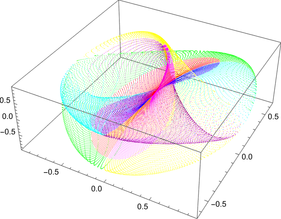
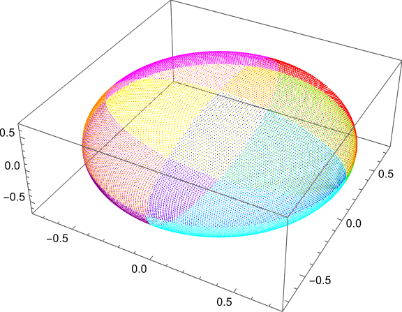
Figure 1: A covering with local coordinates of the hybrid leaf through $(1,2,1)\in\mathbb{R}^{3}$ for $N=4$, $\alpha=0.9$. Left: quantum manifold $\mathcal{M}$, right: embedded quantum space $\tilde{\mathcal{M}}$

In order to verify how well the conditions in (37) are met, in figure 2 the modified relative deviations of the equations are shown, depending on various choices. First, one notes that (37.3) is of much better quality than (37.1) and (37.2) (in fact, it is rescaled according to $m$ in the plots). This has the simple reason that the calculations are pointwise here, while for the other two numerical integration over the leaf is necessary, causing numerical errors.
Further, one sees that the quality improves for $N\to\infty$, $\alpha\to 1$ and $|x|\to\infty$, while the conditions (37) always hold to a satisfactory extent. The choice of distribution is not significant here.

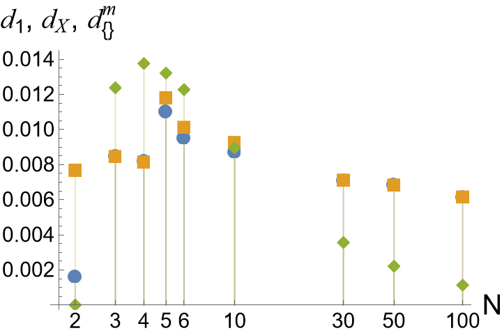
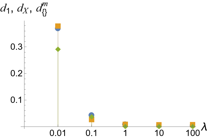
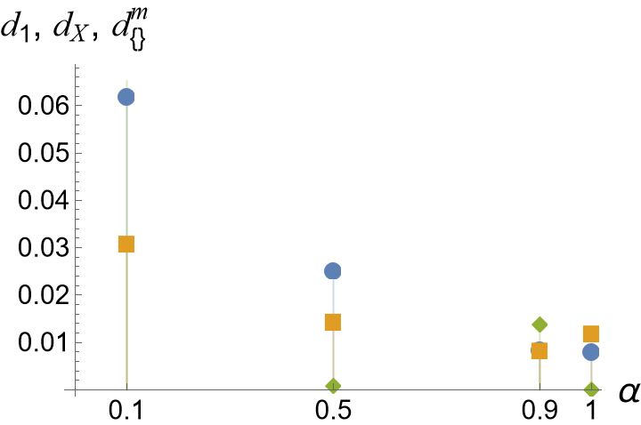
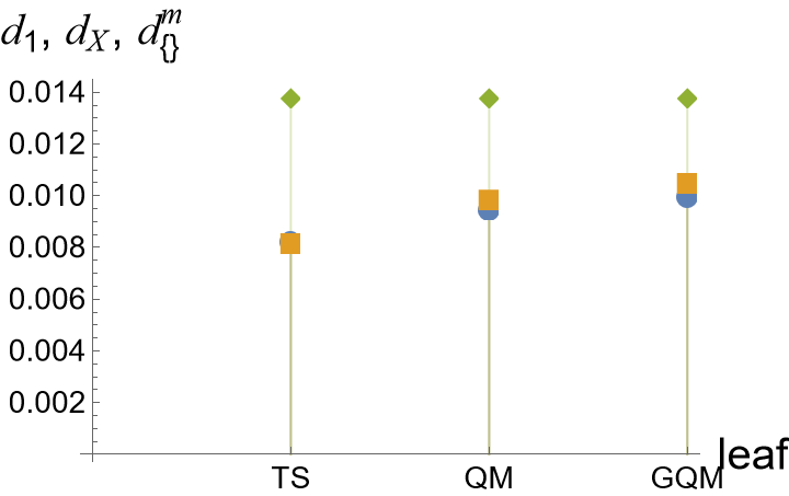
Figure 2: Modified17 relative deviation of (37.1) ($d_{\mathbb{1}}$, blue), (37.2) ($d_{X}$, orange) and (37.3) ($d^{m}_{\{\}}$, green). The generic parameter choice is the setup of figure 1. Top left: dependence on $N$ ($m=100$), top right: dependence on $\alpha$ ($m=100$), bottom left: dependence on the choice of leaf ($m=2$) with $\lambda\cdot(1,2,1)\in\mathbb{R}^{3}$ lying in and hence specifying the leaf, bottom right: dependence on the choice of distribution ($m=100$) with TS being the hybrid leaf, QM being the hybrid leaf using omega and GQM being the same with differently constructed coordinates

4.2 The Perturbed Fuzzy Sphere

Another generalization of the round fuzzy sphere is the perturbed fuzzy sphere.
While for the ordinary sphere $S^{2}$ the space of functions decomposes as $\mathcal{C}(S^{2})\cong\bigoplus_{l=0}^{\infty}(l)$, for the fuzzy sphere the space of modes is truncated $\operatorname{End}(\mathcal{H})\cong\bigoplus_{l=0}^{N-1}(l)$ where in both cases $(l)$ stands for the $2l+1$ dimensional irreducible representation of $SU(2)$, spanned by the classical spherical harmonics $Y_{l}^{m}$ and the fuzzy spherical harmonics $\hat{Y}_{l}^{m}$, respectively.
Given a cutoff $0\leq c\leq N-1$, we randomly choose three hermitian elements ${\cal A}^{a}$ in the span of $\hat{Y}^{l}_{m}$ for $l\leq c$. Given these, we consider the matrix configuration $\tilde{X}^{a}=X^{a}+{\cal A}^{a}$, which defines the perturbed fuzzy sphere of degree $c$.

On the classical side, we can do the same by defining three real valued elements $a^{a}$ in the span of $Y^{l}_{m}$ for $l\leq c$ with the same coefficients and add these to the Cartesian embedding functions $\tilde{x}^{a}:=x^{a}+a^{a}$. The image $(\tilde{x}^{a}(S^{2}))$ then defines a perturbed sphere embedded into $\mathbb{R}^{3}$.

The matrices $A^{a}$ acquire the interpretation of gauge fields on the quantum space $X^{a}$ [20]. Further, the matrix configuration $\tilde{X}^{a}$ is almost local for $c\leq\sqrt{N}$, which is the scale of noncommutativity (NC) on the fuzzy sphere $S^{2}_{N}$. We therefore expect to obtain a good quality of the quantization map below this scale, and bad quality above [1].

In figure 3 we see that the semi-classical limit of the quantum space defined through the hybrid leaf almost perfectly agrees with the classical space. Further, the expected dependence on the cutoff scale is confirmed: for $N=10$ we have $\sqrt{N}\approx 3.2$ and clearly the quality is rather good for $c$ below this scale, while it becomes significantly worse above the NC scale.

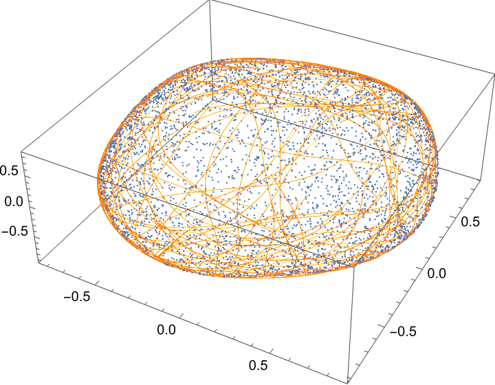
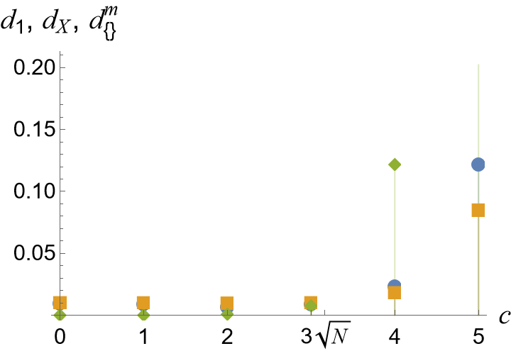
Figure 3: Left: comparison of the classical and quantum space constructed with identical random coefficients, blue: classical space – image of random points on the sphere, orange: embedded quantum space – scan of the hybrid leaf through $(1,2,1)\in\mathbb{R}^{3}$ for $N=10$ and $c=4$, right: plot similar to those of figure 2 depending on $c$ ($m=2$)

4.3 The Fuzzy Torus

The fuzzy torus is an elementary example of a matrix configuration that is not derived from a quantized coadjoint orbit.
For $N>1$, we define $q:=\exp{(2\pi i\frac{1}{N})}\in\mathbb{C}$ and two matrices $U$ and $V$ via $U_{ij}=\delta_{i,j+1}$ respectively $V_{ij}=\delta_{ij}q^{i-1}$. These satisfy the clock and shift algebra

$$q^{N}=1,\quad U^{N}=\mathbb{1}=V^{N},\quad U\cdot V=qV\cdot U.$$ (39)

It is a simple task to see that for $N\to\infty$ this reproduces the algebra $\mathcal{C}(T^{2})$ for the classical torus $T^{2}$ [9].

With that, we set $X^{1}:=\frac{1}{2}(U+U^{\dagger})$, $X^{2}:=\frac{1}{2i}(U-U^{\dagger})$, $X^{3}:=\frac{1}{2}(V+V^{\dagger})$ and $X^{4}:=\frac{1}{2i}(V-V^{\dagger})$, constituting the matrix configuration $(X^{a})$ of the fuzzy torus.
Numerically, for $N>2$ one finds that the maximal rank is $k=3$ while the effective dimension is $l=2$. It is hence unavoidable to consider leaves of $\mathcal{M}$.

In figure 4 we can see that the semi-classical limit defined through the hybrid leaf reproduces a torus to surprising accuracy, already for $N=5$. Further, we find that for $N\to\infty$ the quality of the quantization map improves further, while the conditions of (37) hold to a good extent. This is an important result, since we cannot rely here on group theory to determine $\mathcal{M}$ or ${\cal Q}$, even in the unperturbed case.

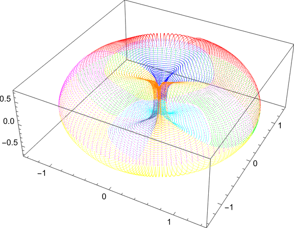
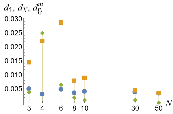
Figure 4: Left: a covering with local coordinates of the hybrid leaf through $(1,2,1,0)\in\mathbb{R}^{3}$ for $N=5$ – a stereographic plot of the embedded quantum space, right: plot similar to those of figure 2 depending on $N$ ($m=0.02$)

4.4 The Squashed Fuzzy $\mathbb{C}P^{2}$

The fuzzy $\mathbb{C}P^{2}$ is a natural 4-dimensional generalization of the fuzzy sphere, replacing $SU(2)$ by $SU(3)$. For given $n\in\mathbb{N}$, we define eight hermitian matrices $T^{a}$ (thus $D=8$) as the orthonormal Lie group generators of $SU(3)$ acting on an orthonormal basis of the irreducible representation $\mathcal{H}_{n}=(n,0)$. Then the dimension of the underlying Hilbert space is $\dim\mathcal{H}_{n}=N=\frac{(n+1)(n+2)}{2}$. Using the quadratic Casimir $C^{2}_{n}=\frac{1}{3}(n^{2}+3n)$, we define the eight matrices

$$X^{a}=\frac{1}{\sqrt{C^{2}_{n}}}T^{a}\ ,$$ (40)

constituting the fuzzy $\mathbb{C}P^{2}$ $(X^{a})$. Since this is again a quantized coadjoint orbit, everything works out perfectly and one finds $\mathcal{L}=\mathcal{M}\cong\mathbb{C}P^{2}$ (thus $k=l=4$) [1, 7].

As for the fuzzy sphere, we can squash fuzzy $\mathbb{C}P^{2}$ by multiplying the matrices $X^{a}$ with some parameters $\alpha_{a}$ to obtain the matrix configuration $\bar{X}^{a}:=\alpha_{a}X^{a}$, which defines the squashed fuzzy $\mathbb{C}P^{2}$. We will focus on the case $\alpha_{3}=\alpha_{8}=\alpha\in[0,1]$ (corresponding to the Cartan generators), with the remaining $\alpha_{a}=1$, respectively where we (randomly) choose $\alpha_{a}$ within $[0,1]$.
Using numerical simulations (for moderate squashing), one finds the maximal rank and the effective dimension to be $k=8$ and $l=4$, reflecting again the oxidation. Therefore the use of foliations is indispensable in order to obtain a semi-classical limit which is stable under perturbation. Unfortunately, due to the increasing numerical expenses, it was not possible to generate a satisfactory covering with local coordinates of the hybrid leaf with the available computational capacity. Thus, we cannot provide significant data on the quality of the semi-classical limit, but we conjecture that the behaviour is very similar to the squashed fuzzy sphere.
What can be done is to look at the image of Cartesian (or other) coordinate lines in target space in order to obtain a global picture of $\mathcal{M}$. Further, the hybrid leaf can be investigated locally by constructing local coordinates. Both is done in figure 5 and we see that in principle the construction still works splendidly.

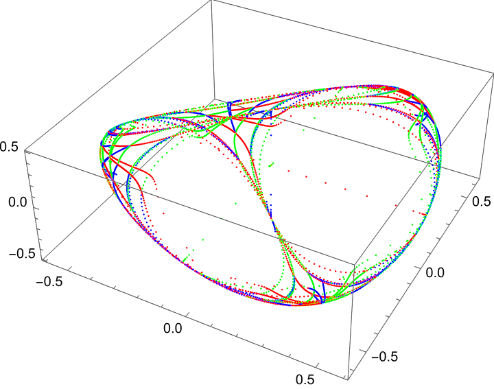
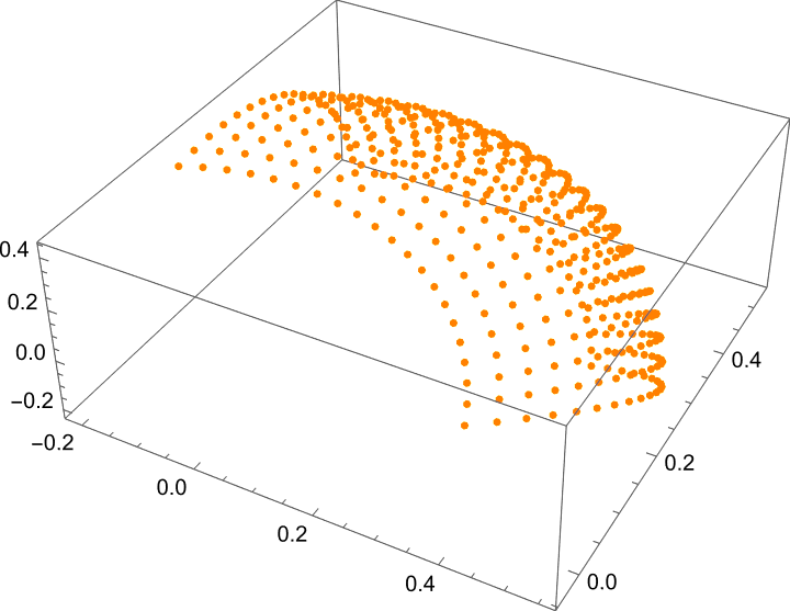
Figure 5: Left: embedded quantum space for $n=3$ – image of Cartesian coordinate lines in target space, right: embedded quantum space for $n=3$ (different perspective) – two directions of local coordinates in the hybrid leaf

5 Conclusion

In this paper, we give a refined definition of a quantum manifold $\mathcal{M}$ which can be associated to any given matrix configuration via quasi-coherent states, generalizing the definition in [1]. In appendix B, this is shown to provide an immersed submanifold in $\mathbb{C}P^{N-1}$. This quantum manifold is endowed with a hermitian form, which defines the quantum metric and the (would-be) symplectic form. This allows to define a preliminary quantization map, which also induces (would-be) Cartesian embedding functions, thus providing the basic ingredients for a semi-classical description of the underlying matrix configuration.
While that construction is perfectly satisfactory e.g. for quantized coadjoint orbits, the construction suffers from oxidation in the general case, leading to a quantum manifold with too many dimensions. We propose some approaches to reduce this quantum manifold to an underlying minimal or irreducible core. In particular, we propose to consider foliations of the quantum manifold, and a restriction to a suitably chosen leaf.
We also study numerically several examples of deformed matrix configurations, where such a restriction is seen to be essential. In particular, one approach to achieve the desired reduction (denoted as hybrid leaf approach) is found to be quite satisfactory, at least numerically. It is both computationally efficient and conceptually appealing, as it turns out to be stable under perturbation; in particular, the variant based on foliations defined by $\omega$ leads by construction to a symplectic form.

Explicit calculations strongly suggest that (at least for large $N$), the hybrid leaf construction leading to $(\mathcal{L},\omega_{\mathcal{L}})$ together with the maps ${\cal Q}:\mathcal{C}(\mathcal{L})\to\operatorname{End}(\mathcal{H})$ and $\mathbf{x}:\mathcal{L}\to\mathbb{R}^{D}$ (approximately) defines a satisfactory semi-classical limit for the given almost local matrix configurations, satisfying the requirements (37). This has been tested for examples derived from quantized coadjoint orbits (the squashed and perturbed fuzzy spheres), but also an example where this is not the case (the fuzzy torus), using the Mathematica package QMGsurvey [11]. Although for the higher dimensional squashed fuzzy $\mathbb{C}P^{2}$ the computational demand has been too high to accurately calculate the quantization map, local coordinates in the hybrid leaf can still be constructed.
We also produce several visualizations for the perturbed fuzzy sphere, which nicely exhibit a meaningful semi-classical limit. The examples also support the conjecture of [7] that the semi-classical limit is of good quality if the cutoff in the $SU(2)$ modes is chosen below the scale of noncommutativity $\sqrt{N}$, but not beyond.
While these results are very encouraging, there are many open problems. Even though the hybrid leaf approach appears to be very promising, it is not yet clear how to properly choose a leaf of the foliation. One may also hope to find other, perhaps iterative procedures which effectively reduce some given matrix configuration to its “irreducible core”, thus reversing the oxidation of the underlying quantized symplectic space through perturbations. In a sense, this problem can be viewed as a noncommutative version of finding optimal Darboux-like coordinates for some given almost-commutative matrix configuration.
Finally, results on the integrability and smoothness of the defining distributions would be very desirable.
The present problem and the methods under discussion should be of considerable interest for numerical simulations of large-$N$ matrix models related to string theory, see e.g. [22, 23]. In particular, they should allow to understand the geometrical meaning of the dominant matrix configurations of such matrix models, and to assess their interpretation in terms of space or space-time.

Acknowledgments

The work of HS is supported by the Austrian Science Fund (FWF) grant P32086.

Appendix A Analyticity of the Eigensystem

Smooth dependence of the quasi-coherent states on $x\in\tilde{\mathbb{R}}^{D}$ is an essential property of the whole construction. For that reason, important results on the analytic and especially smooth dependence of the eigensystem on multiple parameters of a hermitian matrix are summarised here.

Theorem: Let $A:U\subset\mathbb{R}^{n}\to\operatorname{Herm}(\mathcal{H})$ be an analytic function from an open subset $U$ of $\mathbb{R}^{n}$ into the set of hermitian operators on a finite dimensional Hilbert space $\mathcal{H}$. Let $x\in U$ and $\lambda_{x}$ be an eigenvalue of $A(x)$ of multiplicity $1$ with corresponding eigenvector $v_{x}$.
Then, there exists an open neighborhood $V\subset U$ of $x$ and analytic functions $\lambda:V\to\mathbb{R}$ and $v:V\to\mathcal{H}$ such that $\lambda(x)=\lambda_{x}$, $v(x)=v_{x}$ with $\lambda(y)$ being an eigenvalue of $A(y)$ of multiplicity $1$ with corresponding eigenvector $v(y)$ $\forall y\in V$.

This follows from [24] (section 7), generalizing results by Rellich and Kato for a single parameter [25, 26].

The Hamiltonian $H:\mathbb{R}^{D}\to\operatorname{Herm}(\mathcal{H})$ from equation (2.4) obviously is analytic. Thus we can apply the theorem to all points in $\tilde{\mathbb{R}}^{D}:=\{x\in\mathbb{R}^{D}|\operatorname{dim}(E_{x})=1\}$ (with $E_{x}$ being defined as the eigenspace of $H_{x}$ corresponding to the smallest eigenvalue $\lambda_{x}$).
Especially, this implies that $\tilde{\mathbb{R}}^{D}$ is open in $\mathbb{R}^{D}$, the map $\lambda:\tilde{\mathbb{R}}^{D}\to\mathbb{R}$ (assigning the lowest eigenvalue of the Hamiltonian) is smooth and we can locally choose the quasi-coherent states (the corresponding normalized eigenstates) in a smooth way.

Appendix B The Quantum Manifold

In section 2.7 the objects $k$, $\widehat{\mathbb{R}}^{D}$, $\mathcal{M}$ and $q$ have been defined. By construction we deal with a smooth surjection $q:\widehat{\mathbb{R}}^{D}\to\mathcal{M}\subset\mathbb{C}P^{N-1}$ of constant rank $k$.
Therefore, we recall the constant rank theorem:

Theorem: “Suppose $M$ and $N$ are smooth manifolds of dimensions $m$ and $n$, respectively, and $F:M\to N$ is a smooth map with constant rank $r$. For each $p\in M$ there exist smooth charts $(U,\phi)$ for $M$ centered at $p$ and $(V,\psi)$ for $N$ centered at $F(p)$ such that $F(U)\subseteq V$, in which $F$ has a coordinate representation [$\hat{F}=\psi\circ F\circ\phi^{-1}:\phi(U)\to\psi(V)$] of the form $\hat{F}(x^{1},\dots,x^{r},x^{r+1},\dots,x^{m})=(x^{1},\dots,x^{r},0,\dots,0)$.” – theorem 4.12 in [27].

For any $x\in\widehat{\mathbb{R}}^{D}$ the theorem guarantees the existence of corresponding charts $(U,\phi)$ for $\widehat{\mathbb{R}}^{D}$ and $(V,\psi)$ for $\mathcal{M}$. We will use these to define a chart for $\mathcal{M}$, but before we can do so we need two technical lemmas.

In the first lemma we construct a prototypical chart $(\mathcal{U},\bar{\beta}^{-1})$ around $q(x)\in\mathcal{M}$, using the constant rank theorem.

Lemma 1: Consider $q:\widehat{\mathbb{R}}^{D}\to\mathcal{M}\subset\mathbb{C}P^{N-1}$ as in section 2.7. Then for each $x\in\widehat{\mathbb{R}}^{D}$ there exists an open subset $\bar{U}\subset\mathbb{R}^{k}$ and a subset $\mathcal{U}\subset\mathcal{M}$ around $0$ respectively $q(x)$ and a smooth bijection $\bar{\beta}:\bar{U}\to\mathcal{U}$ between them.

Proof: We consider the charts and the map $q^{\prime}:=\psi\circ q\circ\phi^{-1}:\phi(U)\to\psi(V)$, coming from the constant rank theorem.
Now, we define the sets $U^{\prime}:=\phi(U)$, $\mathcal{U}:=q(U)$ and the smooth map $\beta^{\prime}:=q\circ\phi^{-1}:U^{\prime}\to\mathcal{U}$, with $\beta^{\prime}$ being bijective by construction.
Further, $\beta^{\prime}=\psi^{-1}\circ q^{\prime}$ and since $\psi$ is a diffeomorphism, $\beta^{\prime}$ still has constant rank $k$ and depends only on the first $k$ coordinates $\chi^{1},\dots,\chi^{k}$ in $U^{\prime}\subset\mathbb{R}^{D}$.
We define $\bar{U}:=U^{\prime}\cap\mathbb{R}^{k}$ and $\bar{\beta}:=\beta^{\prime}|_{\bar{U}}$.
By shrinking $U$ we can make $\bar{\beta}$ surjective. Since $\bar{\beta}$ has full rank it is an immersion, thus locally injective and we can shrink $U$ once again in order to make $\bar{\beta}$ bijective. $\square$

A little comment on the notation may be helpful. All quantities marked with a prime are related to the space $\mathbb{R}^{D}$ that is the target of the chart $\phi$, while the quantities marked with a bar live on $\mathbb{R}^{k}\cong\mathbb{R}^{k}\times\{0\}\subset\mathbb{R}^{D}$.

Recall $\mathcal{N}_{x}$ from section 2.6. We find that for all $y\in\bar{U}$ the restriction of $\phi^{-1}$ to $\mathcal{N}^{\prime}_{y}:=(\{y\}\times\mathbb{R}^{D-k})\cap U^{\prime}$ is a diffeomorphism from $\mathcal{N}^{\prime}_{y}$ to $\mathcal{N}_{\phi^{-1}(y,0)}\cap U$.
To see this we note that $\phi^{-1}(\mathcal{N}^{\prime}_{y})$ lies within $\mathcal{N}_{\phi^{-1}(y,0)}\cap U$ as $\beta^{\prime}$ is constant here. Further $q^{\prime}$ is injective on $U^{\prime}\cap\mathbb{R}^{k}$, thus only points in $\mathcal{N}^{\prime}_{y}$ are mapped to $\mathcal{N}_{\phi^{-1}(y,0)}\cap U$.

For any $z\in\widehat{\mathbb{R}}^{D}$ this immediately implies $\dim(T_{z}\mathcal{N}_{z})=D-k$, while obviously $T_{z}\mathcal{N}_{z}\subset\operatorname{ker}(T_{z}q)$. Thus, $T_{z}\mathcal{N}_{z}=\operatorname{ker}(T_{z}q)$ what in turn implies that the whole $\mathcal{N}_{z}$ lies within $\widehat{\mathbb{R}}^{D}$.
This leads us to the following lemma which shows that $\mathcal{N}_{W}:=\cup_{x\in W}\mathcal{N}_{x}$ is open in $\widehat{\mathbb{R}}^{D}$ if $W$ is.

Lemma 2: Let $W\subset\widehat{\mathbb{R}}^{D}$. If $W$ is open in $\widehat{\mathbb{R}}^{D}$, then also $\mathcal{N}_{W}$ is open in $\widehat{\mathbb{R}}^{D}$.

Proof: Recall the setup from the proof of lemma 1. Since $\mathcal{N}_{W}\cup\mathcal{N}_{X}=\mathcal{N}_{W\cup X}$, it suffices to show the claim for $W\subset U$. We define $W^{\prime}:=\phi(W)\subset U^{\prime}$ what is clearly open. By the above we find $\mathcal{N}_{W}\cap U=\phi^{-1}((W^{\prime}+\{0\}\times\mathbb{R}^{D-k})\cap U^{\prime})$. Since $\phi$ is a diffeomorphism, this shows that $\mathcal{N}_{W}\cap U$ is open.
Consider now a point $y\in\mathcal{N}_{W}$. By construction there is a $y^{\prime}\in W$ such that $y\in\mathcal{N}_{y^{\prime}}$. Since $\mathcal{N}_{y^{\prime}}$ is convex (see section 2.6), it contains the straight line segment that joins $y$ with $y^{\prime}$.
Then, we can pick ordered points $y_{\alpha}$ for $\alpha=0,\dots,n$ on this line segment with $y_{0}=y^{\prime}$ and $y_{n}=y$ such that the corresponding $U_{\alpha}$ (which we get in the proof of lemma 1 for the point $y_{\alpha}$) cover the line segment (w.l.o.g. we have $U_{\alpha}\cap U_{\beta}\neq\emptyset$ iff $\alpha$ and $\beta$ are consecutive). For $\alpha>0$ we inductively define $W_{\alpha}:=\mathcal{N}_{W_{\alpha-1}}\cap U_{\alpha-1}\cap U_{\alpha}\subset\mathcal{N}_{W}$ with $W_{0}:=W$.
Repeating the above discussion, all $W_{\alpha}$ are open. By construction, all $W_{\alpha}$ contain $\mathcal{N}_{y^{\prime}}\cap U_{\alpha-1}\cap U_{\alpha}$ and are thus nonempty. So finally, $y\in\mathcal{N}_{W_{n}}\cap U_{n}\subset\mathcal{N}_{W}$.
This means that every point $y\in\mathcal{N}_{W}$ has an open neighborhood in $\mathcal{N}_{W}$. $\square$

This result is crucial and allows us to prove that $\mathcal{M}$ is a smooth manifold.

Theorem: $\mathcal{M}$ as defined in section 2.7 is a smooth manifold of dimension $k$.

Proof: By lemma 1 we can cover $\mathcal{M}$ with prototypical charts $(\mathcal{U}_{\alpha},\bar{\beta}_{\alpha}^{-1})$ around $q(x_{\alpha})$ for appropriate points $x_{\alpha}$, defining a prototypical atlas.
Consider now two charts with indices $\beta,\gamma$ such that $\mathcal{U}_{\beta\gamma}:=\mathcal{U}_{\beta}\cap\mathcal{U}_{\gamma}\neq\emptyset$. That the corresponding chart changes are smooth is obvious, but it remains to show that the charts consistently define a topology on $\mathcal{M}$. Then, by lemma 1.35 in [27], $\mathcal{M}$ is a smooth manifold of dimension $k$.
Especially, this means that we have to show that (w.l.o.g.) $\bar{U}_{\beta\gamma}:=\bar{\beta}_{\beta}^{-1}(\mathcal{U}_{\beta\gamma})$ is open in $\mathbb{R}^{k}$.
Since $\bar{U}_{\beta\gamma}\subset\bar{U}_{\beta}$, we only have to show that $\bar{U}_{\beta\gamma}$ is open in the latter. This is equivalent to the statement that there is no sequence in $\bar{U}_{\beta}\setminus\bar{U}_{\beta\gamma}$ that converges against a point in $\bar{U}_{\beta\gamma}$.
Assume to the contrary that such a sequence $(y_{a})$ exists. Since $\phi_{\beta}$ is a diffeomorphism, this defines the convergent sequence $(x_{a}):=(\phi_{\beta}^{-1}(y_{a}))$ in $\widehat{\mathbb{R}}^{D}$ with $\lim_{a\to\infty}x_{a}=:x^{\prime}_{\beta}$. By assumption, $q(x^{\prime}_{\beta})\in\mathcal{U}_{\beta\gamma}$, thus, there is an $x^{\prime}_{\gamma}\in U_{\gamma}$ with $q(x^{\prime}_{\beta})=q(x^{\prime}_{\gamma})$. But then by definition, $x^{\prime}_{\beta}\in\mathcal{N}_{x^{\prime}_{\gamma}}$ and consequently $x^{\prime}_{\beta}\in\mathcal{N}_{U_{\gamma}}$. Since the latter is open by lemma 2, this implies that some $x_{a_{i}}$ lie within $\mathcal{N}_{U_{\gamma}}$. But for these, we find $q(x_{a_{i}})\in\mathcal{U}_{\beta\gamma}$ and consequently $y_{a_{i}}\in\bar{U}_{\beta\gamma}$ what contradicts the assumption. $\square$

Remark: As the rank of $q$ equals $k$ this shows that the inclusion $\mathcal{M}\hookrightarrow\mathbb{C}P^{N-1}$ is an immersion and thus $\mathcal{M}$ is an immersed submanifold of the latter.

If we identify $\mathbb{C}P^{N-1}\cong S^{2N-1}/U(1)$, where $S^{2N-1}\cong\{\ket{\psi}\in\mathbb{C}^{N}|\;\braket{\psi}{\psi}=1\}$, we also get a natural identification of the tangent spaces $T_{U(1)\ket{\psi}}\mathbb{C}P^{N-1}\cong\{\ket{v}\in\mathbb{C}^{N}|\;\braket{\psi}{v}=0\}$.
On the other hand, complex projective space can be viewed as the natural fiber bundle $p:\mathbb{C}^{N}\setminus\{0\}\to\mathbb{C}P^{N-1}$, where in our identification the bundle projection $p$ maps $\ket{\psi}$ to $U(1)\ket{\psi}/\sqrt{\braket{\psi}{\psi}}$, coming with the tangent map $T_{\ket{\psi}}p=(\mathbb{1}-\ket{\psi}\bra{\psi})$.
Then, we get an induced hermitian form $\hat{h}$ on $T\mathbb{C}P^{N-1}$ via $\hat{h}(U(1)\ket{\psi})(\ket{v},\ket{w})=\braket{v}{w}$. By construction, its real part is proportional to the Fubini-Study metric and its imaginary part to the canonical symplectic form on $\mathbb{C}P^{N-1}$, the Kirillov-Kostant-Souriau symplectic form [17].
Since the inclusion $j:\mathcal{M}\hookrightarrow\mathbb{C}P^{N-1}$ is a smooth immersion, we can pull back $\hat{h}$ to $\mathcal{M}$ what we call $h_{\mathcal{M}}=g_{\mathcal{M}}+i\omega_{\mathcal{M}}$, providing us with a metric and an (in general degenerate but closed) would-be symplectic form. Especially, we find $h_{ab}(x):=(q^{*}h_{\mathcal{M}})(x)(\partial_{a},\partial_{b})=h_{\mathcal{M}}(q(x))(T_{x}q\cdot\partial_{a},T_{x}q\cdot\partial_{b})=h_{\mathcal{M}}(q(x))(T_{\tensor[]{\ket{x}}{}}p\cdot\partial_{a}\tensor[]{\ket{x}}{},T_{\tensor[]{\ket{x}}{}}p\cdot\partial_{b}\tensor[]{\ket{x}}{})=h_{\mathcal{M}}(q(x))(D_{a}\tensor[]{\ket{x}}{},D_{b}\tensor[]{\ket{x}}{})=\hat{h}(U(1)\tensor[]{\ket{x}}{})(D_{a}\tensor[]{\ket{x}}{},D_{b}\tensor[]{\ket{x}}{})$
$=(D_{a}\tensor[]{\ket{x}}{})^{\dagger}D_{b}\tensor[]{\ket{x}}{}$, where we described $q=p\circ\tensor[]{\ket{\cdot}}{}$ via a local section and used $D_{a}\tensor[]{\ket{x}}{}=(\mathbb{1}-\tensor[]{\ket{x}}{}\tensor[]{\bra{x}}{})\partial_{a}\tensor[]{\ket{x}}{}=T_{\tensor[]{\ket{x}}{}}p\cdot\partial_{a}\tensor[]{\ket{x}}{}$.
But this means that the pullback of $h_{\mathcal{M}}$ along $q$ agrees with the $h_{ab}$ we have defined earlier, similarly for $g_{\mathcal{M}}$ and $\omega_{\mathcal{M}}$.

References

- [1] Harold C. Steinacker “Quantum (matrix) geometry and quasi-coherent states” In Journal of Physics A: Mathematical and Theoretical 54.5, 2021, pp. 055401 arXiv:2009.03400 [hep-th]
- [2] Nobuyuki Ishibashi, Hikaru Kawai, Yoshihisa Kitazawa and Asato Tsuchiya “A large-N reduced model as superstring” In Nuclear Physics B 498.1-2, 1997, pp. 467 arXiv:9612115 [hep-th]
- [3] Tom Banks, W. Fischler, S.. Shenker and Leonard Susskind “M theory as a matrix model: A Conjecture” In Phys. Rev. D55, 1997, pp. 5112–5128 DOI: 10.1103/PhysRevD.55.5112
- [4] Harold C. Steinacker “Emergent gravity on covariant quantum spaces in the IKKT model” In Journal of High Energy Physics 2016.12, 2016, pp. 156 arXiv:1606.00769 [hep-th]
- [5] Goro Ishiki “Matrix Geometry and Coherent States” In Phys. Rev. D92.4, 2015, pp. 046009 DOI: 10.1103/PhysRevD.92.046009
- [6] Askold Perelomov “Generalized Coherent States and Their Applications” Berlin, Heidelberg: Springer, 1986
- [7] Laurin J. Felder “Quasi-Coherent States on Deformed Quantum Geometries”, 2023 arXiv:2301.10206 [hep-th]
- [8] Lukas Schneiderbauer “Semi-classical and numerical aspects of fuzzy brane solutions in Yang-Mills theories”, 2015
- [9] Lukas Schneiderbauer and Harold C. Steinacker “Measuring finite quantum geometries via quasi-coherent states” In Journal of Physics A: Mathematical and Theoretical 49.28, 2016, pp. 285301 arXiv:1601.08007 [hep-th]
- [10] David Berenstein and Eric Dzienkowski “Matrix embeddings on flat and the geometry of membranes” In Phys. Rev. D 86, 2012, pp. 086001 DOI: 10.1103/PhysRevD.86.086001
- [11] Laurin J. Felder “(GitHub) laurinjfelder/QMGsurvey: Initial Release” Zenodo, 2023 URL: https://doi.org/10.5281/zenodo.7941284
- [12] Harold C. Steinacker “Fuzzy spaces and applications” Lecture notes University of Vienna, 2016
- [13] Stefan Waldmann “Poisson-Geometrie und Deformationsquantisierung” Berlin, Heidelberg: Springer, 2007
- [14] Peter W. Michor “Topics in differential geometry” Providence, Rhode Island: American Mathematical Society, 2008
- [15] Julia Bernatska and Petro Holod “Geometry and Topology of Coadjoint Orbits of Semisimple Lie Groups” In Proceedings of the Ninth International Conference on Geometry, Integrability and Quantization 1 Sofia: Bulgarian Academy of Sciences, 2008, pp. 141
- [16] Karl-Hermann Neeb “Holomorphic Representations and Coherent States” In Quantization and Infinite-Dimensional Systems 1 New York: Springer, 1994, pp. 79
- [17] Bertram Kostant and Shlomo Sternberg “Symplectic Projective Orbits” In New Directions in Applied Mathematics: Papers Presented April 25/26, 1980, on the Occasion of the Case Centennial Celebration 1 New York, Heidelberg, Berlin: Springer, 1982, pp. 81
- [18] John A. Madore “The fuzzy sphere” In Classical and Quantum Gravity 9.1, 1992, pp. 69
- [19] J.. Hoppe “Quantum Theory of a Massless Relativistic Surface and a Two-Dimensional Bound State Problem.”, 1982
- [20] Harold C. Steinacker and Jochen Zahn “Self-intersecting fuzzy extra dimensions from squashed coadjoint orbits in N=4 SYM and matrix models” In Journal of High Energy Physics 2015.2, 2015, pp. 27 arXiv:1409.1440 [hep-th]
- [21] Richard Shurtleff “Formulas for SU(3) Matrices”, 2009 arXiv:0908.3864 [math-ph]
- [22] Jun Nishimura “Signature change of the emergent space-time in the IKKT matrix model” In PoS CORFU2021, 2022, pp. 255 DOI: 10.22323/1.406.0255
- [23] Jun Nishimura, Toshiyuki Okubo and Fumihiko Sugino “Systematic study of the SO(10) symmetry breaking vacua in the matrix model for type IIB superstrings” In JHEP 10, 2011, pp. 135 DOI: 10.1007/JHEP10(2011)135
- [24] Krzysztof Kurdyka and Laurentiu Paunescu “Hyperbolic polynomials and multiparameter real-analytic perturbation theory” In Duke Mathematical Journal 141.1, 2008, pp. 123 arXiv:0602538 [math]
- [25] Franz Rellich and Brian Berkowitz “Perturbation Theory of Eigenvalue Problems” CRC Press, 1969
- [26] Tosio Kato “Perturbation Theory for Linear Operators” Berlin, Heidelberg: Springer, 1995
- [27] John M. Lee “Introduction to Smooth Manifolds” New York, Heidelberg, Dordrecht, London: Springer, 2003