P-tensors: a General Formalism for Constructing Higher Order Message Passing Networks

Abstract

Several recent papers have recently shown that higher order graph neural networks can achieve better accuracy than their standard message passing counterparts, especially on highly structured graphs such as molecules. These models typically work by considering higher order representations of subgraphs contained within a given graph and then perform some linear maps between them. We formalize these structures as permutation equivariant tensors, or P-tensors, and derive a basis for all linear maps between arbitrary order equivariant P-tensors. Experimentally, we demonstrate this paradigm achieves state of the art performance on several benchmark datasets.

1 Introduction

In recent years, neural networks have been employed and even become common place across many different fields, being applied to many different types of data, especially graphs. Many different approaches for learning on graphs originate from areas such as computer vision and natural language processing, which can be thought of special cases of graph learning where the data appears as paths or grids, rather than arbitrary graphs. One of the most popular family of graph neural networks (GNNs) are the so called Message Passing Neural Networks (MPNNs) [14], which learn on graphs by by having vertices transfer information between them as “messages”. However, this paradigm has provably limited expressive power [25][33], prompting the creation of more powerful models that can provide richer representations of graphs [23][24][22][12]. In particular, [23] gives the number of linear maps within higher order representations (tensors). In this work, we will generalize this to give a basis of equivariant linear maps between tensors of different reference domains. This allows for GNNs to pass messages between arbitrary subgraphs, rather than be restricted to vertices or hyperedges [22][23].

2 Background: permutation equivariant neural networks

Let $\mathcal{G}$ be an undirected graph with $n$ vertices and $A\in\mathbb{R}^{n\times n}$ its adjacency matrix. Graph neural networks (GNNs) learn a function $\Phi\colon A_{\mathcal{G}}\mapsto\Phi(A_{\mathcal{G}})$ embedding such graphs in some Euclidean space $\mathbb{R}^{D}$. The representation of graphs by adjacency matrices however is not unique. If we change the order in which the vertices of $\mathcal{G}$ are numbered by a permutation $\sigma$, $A$ transforms to $A^{\prime}$, where

$$[A^{\prime}]_{i,j}=A_{\sigma^{-1}(i),\sigma^{-1}(j)}.$$ (1)

From the point of view of graph topology, however $A$ and $A^{\prime}$ still correspond to the same underlying graph $\mathcal{G}$. This forces the constraint $\Phi(A)=\Phi(A^{\prime})$ on any graph neural network.

The principle challenge in GNNs is to design architectures that respect this invariance constraint, yet are expressive enough to capture the complex topological features demanded by applications. One way to enforce permutation invariance would be to compute permutation invariant graph features right in the input layer. Whatever the architecture of the rest of the network, this would guarantee that the output is permutation invariant. This approach, however severely limits the expressive power of the network [22][29]. Instead, modern GNNs are designed in such a way that their internal layers are equivariant (rather than invariant) to permutations. This means that under (1) the outputs of the layers do change, but they do so in specific, controlled ways. The final layer of the network is designed to cancel out these transformations and guarantee that the overall output of the network is permutation invariant.

Technically, (1) describes the action of the symmetric group ${\mathbb{S}_{n}}$ (the group of permutations of $n$ objects) on the adjacency matrix. However, ${\mathbb{S}_{n}}$ has many other actions on various different types of objects. The critical constraint in equivariant GNNs is that output $f^{\ell}$ of each layer must transform according to a specific, pre-determined action $\mathcal{T}^{\ell}$ of ${\mathbb{S}_{n}}$. Equivalently, each layer $\phi^{\ell}$, regarded as a (learned) mapping $\phi^{\ell}\colon f^{\ell-1}\mapsto f^{\ell}$ must be a permutation equivariant map, meaning that $\phi^{\ell}(\mathcal{T}^{\ell-1}_{\sigma}(f))=\mathcal{T}^{\ell}_{\sigma}(\phi^{\ell}(f))$ for any $f$ and any permutation $\sigma$.

2.1 Message passing networks

Several, seemingly very different approaches have emerged to building equivariant graph neural nets [16][18][13][25]. Arguably the most popular approach however is that of Message Passing Neural Nets (MPNNs) [14]. A unique feature of MPNNs is that the titular “neurons” are attached to the vertices of the graph itself and that the way that these neurons communicate with each other is to send “messages” to each other in a way that is dictated by the graph topology. In the simplest case, the output of the neuron at each vertex $i$ in layer $\ell$ is a vector $f_{i}^{\ell}\in\mathbb{R}^{D_{\ell}}$, and the update rule is

$$f^{\ell}_{i}=\eta\Bigl{(}W_{\ell}\!\sum_{j\in\mathcal{N}(i)}f^{\ell-1}_{j}+b^{\ell}_{i}\Bigr{)},$$ (2)

where $\mathcal{N}(i)$ denotes the neighbors of node $i$, $W_{\ell}$ is a learnable weight matrix, $b^{\ell}_{i}$ is a learnable bias term and $\eta$ is a pointwise non-linearity. By itself, (2) does not look like a permutation equivariant operation, since it explicitly differentiates between two categories of vertices: those that are neighbors of vertex $i$ and those that are not. The reason that MPNNs nonetheless manage to be permutation equivariant is that this distinction itself covariance with permutations: if vertices $i$ and $j$ are neighbors before permutation, then after permuting the vertices by $\sigma$, vertex $\sigma(i)$ will be a neighbor of $\sigma(j)$. Hence, (2) is an update rule informed by side information (the neighborhood relationships between vertices) which itself covariance with permutations. This property is key to the MPNN update rule being powerful, yet still equivariant.

2.2 Higher order message passing and two-level equivariance

Despite their popularity, simple message passing neural networks do have their limitations, the most obvious of which is that, each vertex $i$ just sums all the incoming messages from its neighbors. Summation is an associative and commutative operation, without which MPNNs would not be equivariant. On the other hand, these same properties also make MPNNs myopic: once the activations have been summed together, the neuron at vertex $i$ cannot distinguish between which part of the incoming message came from which neighbor. If in the following layer some of the same vertices are featured again, the algorithm cannot identify them with the messages coming from individual vertices in layer $\ell-1$. This fact has been noted in several papers [25][33][7] and is a fundamental limitation on the representational capacity of MPNNs, closely related to the findings of a sequence of theoretical studies analyzing the universality properties of GNNs in relation to the famous Weisfeiler-Leman test for graph isomorphism [33][32]. On an intuitive level, MPNNs are good at locally propagating information on graphs, loosely like convolution, but are not so good at capturing important local structures. This is especially problematic in applications like organic chemistry, where the local subgraphs have explicit meaning as e.g., functional groups.

In response to these criticisms, several authors have proposed variations on the message passing paradigm where individual neurons correspond to not just single vertices, but sets of vertices, or rather, subgraphs. Such “super-neurons” have the ability to represent information relating to the entire subgraph, including relations between the vertices of the subgraph, almost as a “GNN within a GNN”. Correspondingly, the output of such a “super-neuron” is a vector, matrix or tensor, transforming in specific ways according to the internal permutations of the vertices that it is responsible for. For example, if the subgraph in question is a triangle consisting of vertices $(i_{1},i_{2},i_{3})$, the output might be a 3-index quantity $T\in\mathbb{R}^{3\times 3\times C}$. If we permute the three vertices of the triangle by a local permutation $\tau\in\mathbb{S}_{3}$, $T$ transforms to $T^{\prime}_{i,j,c}=T_{\tau^{-1}(i),\tau^{-1}(j),c}.$ Architectures of this type we call higher order message passing networks.

In such networks equivariance comes into play at two separate levels: globally, at the level of the subgraphs corresponding to different neurons being permuted with each other, and locally, at the level of the vertices belonging to an individual subgraph being permuted amongst themselves. In this paper we develop a general mathematical formalism for describing this situation an derive the most general form of message passing operations that ensures overall equivariance (Figure 1).

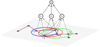
Figure 1: In higher order message passing networks, permutation equivariance acts on two levels: (a) it affects which vertices a given neuron $\mathfrak{n}$ is responsible for (the referenced domain $\mathcal{D}_{\mathfrak{n}}$), and (b) it changes the ordering of the vertices in $\mathcal{D}_{\mathfrak{n}}$ itself. Equivariance with respect to the first transformation is relatively easy to achieve, simply by ensuring that the policy used to select the reference domain is itself permutation covariant [12]. The second type of transformation is more subtle and requires the P-tensor formalism to account for.

3 P-tensors

The mathematical device that we introduce in this paper to derive the rules of higher order message passing are a type of object that we call P-tensors. To define $P$-tensors we must first define a finite or countably infinite set $\mathcal{U}$ of base objects called atoms that permutations act on. In the case of graph neural networks, the atoms are just the vertices of $\mathcal{G}$. In more general forms of relational learning, $\mathcal{U}$ might for example be a set of individuals or the words in a given language.

A P-tensor $T$ is always defined relative to an ordered subset $\mathcal{D}$ of atoms called its reference domain. In the case of subgraph neurons, $\mathcal{D}$ would just be the vertices of the subgraph.

Definition 1 (P-tensors).

Let $\mathcal{U}$ be a finite or countably infinite set of atoms and $\mathcal{D}=(x_{1},\ldots,x_{d})$ an ordered subset of $\mathcal{U}$. We say that a $k$’th order tensor $T\in\mathbb{R}^{d\times d\times\ldots\times d}$ is a $k$’th order permutation covariant tensor (or P-tensor for short) with reference domain $\mathcal{D}$ if under the action of a permutation $\tau\in\mathbb{S}_{d}$ acting on $\mathcal{D}$ it transforms as

$$\tau(T)_{i_{1},i_{2},\ldots,i_{k}}=T_{\tau^{-1}(i_{1}),\ldots\tau^{-1}(i_{k})}.$$ (3)

The neurons in modern neural networks typically have many channels, so we allow P-tensors to also have a channel dimension. Thus, a $k$’th order P-tensor can actually be a $k+1$’th order tensor $\smash{T\in\mathbb{R}^{d\times d\times\ldots\times d\times C}}$. The channel dimension is not affected by permutations.

P-tensors are defined with reference to permutations acting on their own reference domain. Ultimately, however, we are interested in how to send messages between two P-tensors in a way that is equivariant to both their reference domains being permuted simultaneously, in a coordinated way. Defining what we mean by this precisely brings us back to the notion of two-level equivariance mentioned at the end of the previous section. To describe equivariant message passing from one P-tensor $T_{1}$ to a second P-tensor $T_{2}$ we need to consider global permutations $\sigma$ of $\mathcal{U}$ that fix their reference domains $\mathcal{D}_{1}$ and $\mathcal{D}_{2}$ as sets, but may change the relative ordering of $\mathcal{D}_{1}$ w.r.t. $\mathcal{D}_{2}$, denoted by $\tau$. To make these notions precise, we need the following definitions.

Definition 2 (Action of global permutations).

Let $\mathcal{U}=\{x_{1},x_{2},\ldots\}$ be a finite or countably infinite set of atoms and $\sigma$ be a permutation of the elements of  $\mathcal{U}$  so that $x^{\prime}_{i}=x_{\sigma^{-1}(i)}$. Given an ordered subset $\mathcal{D}=(x_{i_{1}},\ldots,x_{i_{d}})$ of  $\mathcal{U}$, we define $\smash{\sigma(\mathcal{D})=(x_{\sigma^{-1}(i_{1})},\ldots,x_{\sigma^{-1}(i_{d})})}$.

Definition 3 (Fixed sets and restricted permutations).

We say that $\sigma$ fixes $\mathcal{D}$ (as a set) if $\mathcal{D}$ and $\sigma(\mathcal{D})$ are equal as sets (denoted $\smash{\mathcal{D}\mathop{\stackrel{{\scriptstyle\textrm{set}}}{{=}}}{}\sigma(\mathcal{D})}$), i.e., if

$$\sigma(\mathcal{D}):=(x_{\sigma^{-1}(i_{1})},\,x_{\sigma^{-1}(i_{2})},\,\ldots\,,x_{\sigma^{-1}(i_{d})})=(x_{i_{\tau^{-1}(1)}},\ldots,x_{i_{\tau^{-1}(d)}})$$

for some permutation $\tau\in\mathbb{S}_{d}$. We say that $\tau$ is the restriction of $\sigma$ to $\mathcal{D}$ and denote it $\tau=\sigma{\downarrow}_{\mathcal{D}}$.

Clearly, $\tau=\sigma{\downarrow}_{\mathcal{D}}$, when it exists, must satisfy $\smash{\sigma(i_{j})=i_{\tau(j)}}$ for all $j$. Moreover, if the original $\mathcal{D}$ is written as $\smash{\mathcal{D}=\left(\overline{x}_{1},\ldots,\overline{x}_{d}\right)}$, whenever $\mathcal{D}$ is fixed by $\sigma$, its permuted version can be written as just $\sigma(\mathcal{D})=(\overline{x}_{\tau^{-1}(1)},\overline{x}_{\tau^{-1}(2)},\ldots,\overline{x}_{\tau^{-1}(d)})$. We are now in a position to define what it means for a map $\phi\colon T_{1}\mapsto T_{2}$ between two P-tensors to be equivariant.

Definition 4 (Equivariant map between P-tensors).

Let $T_{1}$ and $T_{2}$ be two P-tensors with reference domains $\mathcal{D}_{1}\subseteq\mathcal{U}$ and $\mathcal{D}_{2}\subseteq\mathcal{U}$, respectively, and $\phi$ be a map from $T_{1}$ to $T_{2}$. We say that $\phi$ is a permutation equivariant map if

$$\phi(\sigma{\downarrow}_{\mathcal{D}_{1}}(T_{1}))=\sigma{\downarrow}_{\mathcal{D}_{2}}(\phi(T_{1}))$$

for all permutations $\sigma$ of $\mathcal{U}$ that fixes both $\mathcal{D}_{1}$ and $\mathcal{D}_{2}$ as sets.

While seemingly abstract, these definitions capture exactly how higher order quantities related to different but potentially overlapping sets of objects are expected to behave under permutations, in particular, how the activations of a higher order MPNN change under permutations of the vertices. In line with much of the literature on neural networks with generalized convolution-type operations on various objects, in the following we focus on deriving the most general linear equivariant operations between P-tensors. We do this in two steps: first we consider the case that $\smash{\mathcal{D}_{1}\mathop{\stackrel{{\scriptstyle\textrm{set}}}{{=}}}{}\mathcal{D}_{2}}$, and then the more general case where $\mathcal{D}_{1}$ and $\mathcal{D}_{2}$ overlap only partially.

3.1 Message passing between P-tensors with the same reference domain

If $\mathcal{D}_{1}=(x_{1},\ldots,x_{d})$ and $\mathcal{D}_{2}=(x^{\prime}_{1},\ldots,x^{\prime}_{d})$ are equal as sets, they can only differ by a hidden permutation $\mu$, mapping $x^{\prime}_{1}=x_{\mu(1)}$ $x^{\prime}_{2}=x_{\mu(2)}$, and so on. In a graph neural network, determining whether two labels refer to the same underlying vertex is always possible, so a GNN can always find the correct $\mu$ that maps one set onto the other. Without loss of generality, we therefore assume that the elements of $\mathcal{D}_{2}$ have already been rearranged so that $x_{1}^{\prime}=x_{1}$,…$x_{d}^{\prime}=x_{d}$. This reduces the problem to that of “ordinary” permutation equivariant vector, matrix, etc., valued neural network layers, which, by now, is a well studied subject.

In the first order case, the P-tensors are simply vectors, so we are just asking what the most general linear map $\phi\colon\mathbb{R}^{d}\to\mathbb{R}^{d}$ is that satisfies

$$\phi([\textbf{{v}}]_{\tau^{-1}(i)})=[\phi(\textbf{{v}})]_{\tau^{-1}(i)}$$

for any $\textbf{{v}}\in\mathbb{R}^{d}$ and any $\tau\in\mathbb{S}_{d}$. The seminal Deep Sets paper [35] proved that in this case $\phi$ can have at most two (learnable) parameters $\lambda_{1}$ and $\lambda_{2}$, and must be of the form

$$\phi(\textbf{{v}})=\lambda_{1}\textbf{{v}}+\lambda_{2}\mbox{\boldmath$1$}\hskip 1.00006pt\mbox{\boldmath$1$}^{\top}\!\textbf{{v}}.$$

In the more general case, $\phi$ maps a $k_{1}$’th order tensor $T^{\textrm{in}}$ to a $k_{2}$’th order tensor $T^{\textrm{out}}$, both transforming under permutations as in (3), leading to the equivariance condition

$$[\phi(T^{\textrm{in}})]_{\tau^{-1}(i_{1}),\ldots,\tau^{-1}(i_{k_{2}})}=\phi(T^{\textrm{in}}_{\tau^{-1}(i_{1}),\ldots,\tau^{-1}(i_{k_{1}})}).$$ (4)

The characterization of the space of equivariant maps for this case was given in a similarly influential paper by Maron et al. [23].

Proposition 1 (Maron et al.).

The space of linear maps $\smash{\phi\colon\mathbb{R}^{d^{k_{1}}}\to\mathbb{R}^{d^{k_{2}}}}$ that is equivariant to permutations $\tau\in\mathbb{S}_{d}$ in the sense of (4) is spanned by a basis indexed by the partitions of the set $\{1,2,\ldots,k_{1}+k_{2}\}$.

Since the number of partitions of $\{1,2,\ldots,m\}$ is given by the so-called Bell number $B(m)$, according to this result, the number of learnable parameters in such a map is $B(k_{1}+k_{2})$. Each equivariant linear map corresponding to one of the partitions can be thought of as a composition of three operations: (1) summing over specific dimensions or diagonals of $T^{\textrm{in}}$; (2) transferring this result to the output tensor by identifying some combinations of input indicies with output indices; (3) broadcasting the result along certain dimensions or diagonals of the output tensor $T^{\textrm{out}}$. These three operations correspond to the three different types of sets that can occur in a given partition $\mathcal{P}$: those that only involve the second $k_{2}$ numbers, those that involve a mixture of the first $k_{1}$ and second $k_{2}$, and those that only involve the first $k_{1}$. We shall say that $\mathcal{P}$ is of type $(p_{1},p_{2},p_{3})$ if it has $p_{3}$ sets of the first category, $p_{2}$ in the second and $p_{1}$ in the third. In all three categories, the rule is that a given set $\{j_{1},\ldots,j_{\ell}\}$ appearing in $\mathcal{P}$ means that the corresponding indices are tied together. The way to distinguish between input and output indices is that if $1\leq j_{q}\leq k_{1}$ then it refers to the $j_{q}$’th index of $T^{\textrm{out}}$, whereas if $k_{1}+1\leq j_{q}\leq k_{1}+k_{2}$, then it refers to the $j_{q}-k_{1}$ index of $T^{\textrm{in}}$.

As an example, in the $k_{1}=k_{2}=3$ case, the $\mathcal{P}=\{\{1,3\},\{2,5,6\},\{4\}\}$ partition corresponds to (a) summing $T^{\textrm{in}}$ along its first dimension (corresponding to $\{4\}$) (b) transferring the diagonal along the second and third dimensions of $T^{\textrm{in}}$ to the second dimension of $T^{\textrm{out}}$ (corresponding to $\{2,5,6\}$), (c) broadcasting the result along the diagonal of the first and third dimensions (corresponding to $\{1,3\}$). Explicitly, this gives the equivariant map

$$T^{\textrm{out}}_{a,b,a}=\sum_{c}T^{\textrm{in}}_{c,b,b}.$$ (5)

Since $B(6)=203$, listing all other possible maps for $k_{1}=k_{2}=3$ would be very laborious. As an illustration, in Table 1 we just list the possible equivariant maps for the $k_{1}=k_{2}=2$ case.

$$\begin{array}[]{|c|c|}\hline\cr\mathcal{P}&\phi\\ \hline\cr\{\{1\},\{2\},\{3\},\{4\}\}&T^{\textrm{out}}_{a,b}=\sum_{c,d}T^{\textrm{in}}_{c,d}\\ \{\{1\},\{2\},\{3,4\}\}&T^{\textrm{out}}_{a,b}=\sum_{c}T^{\textrm{in}}_{c,c}\\ \{\{1\},\{2,4\},\{3\}\}&T^{\textrm{out}}_{a,b}=\sum_{c}T^{\textrm{in}}_{c,b}\\ \{\{1\},\{2,3\},\{4\}\}&T^{\textrm{out}}_{a,b}=\sum_{c}T^{\textrm{in}}_{b,c}\\ \{\{2\},\{1,4\},\{3\}\}&T^{\textrm{out}}_{b,a}=\sum_{c}T^{\textrm{in}}_{c,b}\\ \{\{2\},\{1,3\},\{4\}\}&T^{\textrm{out}}_{b,a}=\sum_{c}T^{\textrm{in}}_{b,c}\\ \{\{1,2\},\{3\},\{4\}\}&T^{\textrm{out}}_{a,a}=\sum_{b,c}T^{\textrm{in}}_{b,c}\\ \{\{1\},\{2,3,4\}\}&T^{\textrm{out}}_{a,b}=T^{\textrm{in}}_{b,b}\\ \hline\cr\end{array}\hskip 20.0pt\begin{array}[]{|c|c|}\hline\cr\mathcal{P}&\phi\\ \hline\cr\{\{2\},\{1,3,4\}\}&T^{\textrm{out}}_{b,a}=T^{\textrm{in}}_{b,b}\\ \{\{1,2,3\},\{4\}\}&T^{\textrm{out}}_{a,a}=\sum_{b}T^{\textrm{in}}_{a,b}\\ \{\{1,2,4\},\{3\}\}&T^{\textrm{out}}_{a,a}=\sum_{b}T^{\textrm{in}}_{b,a}\\ \{\{1,2\},\{3,4\}\}&T^{\textrm{out}}_{a,a}=\sum_{c}T^{\textrm{in}}_{c,c}\\ \{\{1,3\},\{2,4\}\}&T^{\textrm{out}}_{a,b}=T^{\textrm{in}}_{a,b}\\ \{\{1,4\},\{2,3\}\}&T^{\textrm{out}}_{a,b}=T^{\textrm{in}}_{b,a}\\ \{\{1,2,3,4\}\}&T^{\textrm{out}}_{a,a}=T^{\textrm{in}}_{a,a}\\ \hline\cr\end{array}$$

Table 1: The $B(4)=15$ possible partitions of the set $\{1,2,3,4\}$ and the corresponding permutation equivariant linear maps $\phi:\mathbb{R}^{k\times k}\to\mathbb{R}^{k\times k}$ as derived by Maron et al. [23].

The presence of multiple channels enriches this picture only to the extent that each input channel can be linearly mixed with each output channel. For example, in the case of $C_{\textrm{in}}$ channels in $T^{\textrm{in}}$ and $C_{\textrm{out}}$ channels in $T^{\textrm{out}}$, (5) becomes

$$T^{\textrm{out}}_{a,b,a,\alpha}=\sum_{\beta}W_{\alpha,\beta}\sum_{c}T^{\textrm{in}}_{c,b,b,\beta}$$

for some (learnable) weight matrix $W\in\mathbb{R}^{C_{\textrm{out}}\times C_{\textrm{in}}}$. Note that this type of linear mixing across channels is very general and can be separated from the equivariant message passing operation itself, which in this case is is really just (5) applied to every single channel separately.

3.2 Message passing between P-tensors with different reference domains

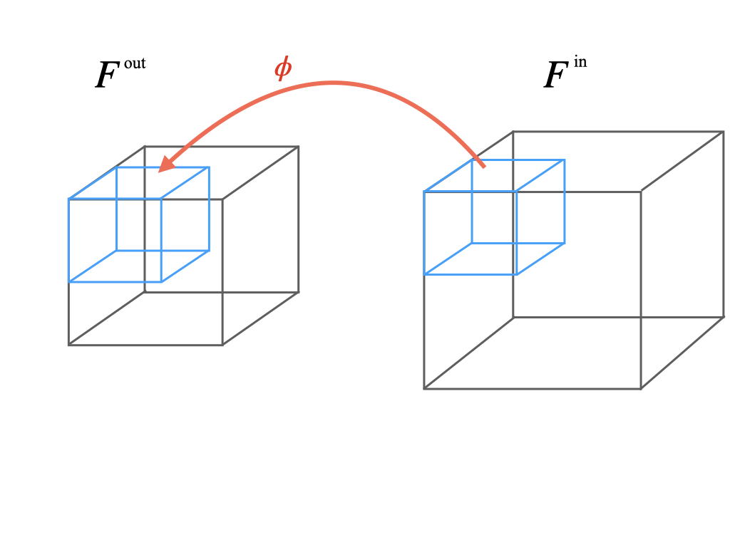
$$\small\begin{array}[]{|c|c|c|}\hline\cr(k_{1},k_{2})&\pbox{100pt}{\#ofmapsin\\ $ $\mathcal{D}$_1\mathop{\stackrel{{\scriptstyle{set}}}{{=}}}$\mathcal{D}$_2 $case}&\pbox{100pt}{\#ofmapsin\\ $ $\mathcal{D}$_1\not{\!\mathop{\stackrel{{\scriptstyle{set}}}{{=}}}}$\mathcal{D}$_2 $case}\\ \hline\cr(0,0)&1&1\\ (1,1)&2&17\\ (1,2)&5&49\\ (2,2)&15&129\\ (2,3)&52&321\\ (3,3)&203&769\\ \hline\cr\end{array}$$

Figure 2: Left: Given two P-tensors $T^{\textrm{in}}$ and $T^{\textrm{out}}$ whose reference domains have $d^{\cap}$ atoms in common, without loss of generality we can rearrange the two tensors so that the indices corresponding to the common atoms appear first. Mapping the corresponding $d^{\cap}\!\times d^{\cap}\!\times\ldots\times d^{\cap}$ subtensor of $T^{\textrm{in}}$ to the analogous $d^{\cap}\!\times d^{\cap}\!\times\ldots\times d^{\cap}$ subtensor of $T^{\textrm{out}}$ with any of the $B(k_{1}+k_{2})$ linear maps described in Section 3.1 is an equivariant operation in the sense of Definition 4. Right: In the case of partially overlapping reference domains, if the given type of equivariant map involves either summing over certain dimensions from the input tensor or broadcasting over certain dimensions in the ouput tensor, the same map is going to have $2^{p_{1}+p_{3}}$ variants corresponding to whether the summation/broadcating only extends over the common atoms or not. This gives rise to may more possible equivariant maps.

One of the main results of the present paper is the following Theorem, which generalizes Proposition 1 to the case when the reference domains of the input and output tensors only partially overlap.

Theorem 2.

Let $T_{1}$ and $T_{2}$ be two P-tensors with reference domains $\mathcal{D}_{1}$ and $\mathcal{D}_{2}$ such that $\mathcal{D}_{1}\cap\mathcal{D}_{2}\neq\emptyset$ and $\mathcal{D}_{1}\not\subseteq\mathcal{D}_{2}$ and $\mathcal{D}_{2}\not\subseteq\mathcal{D}_{1}$. The set of all linearly independent maps from $T_{1}$ to $T_{2}$ is given by the set of pairs of partitions $\mathcal{P}_{1}$ and $\mathcal{P}_{2}$, from any subset of $[k]$ and $[k^{\prime}]$. respectively.

To derive the form of the actual maps, without loss of generality, we assume that $\mathcal{D}_{1}$ and $\mathcal{D}_{2}$ have been reordered so that their $d^{\cap}=|\mathcal{D}_{1}\cap\mathcal{D}_{2}|$ common atoms occupy the first $d^{\cap}$ positions in both, and are listed in the same order. An easy generalization of our previous results is then to associate to each partition the same map as before, except we now only transfer information from the subtensor of $T^{\textrm{in}}$ cut out by the common atoms to the subtensor of $T^{\textrm{out}}$ cut out by the same (Figure 2 left). For example, the counterpart of (5) would be

$$T^{\textrm{out}}_{a,b,a}=\begin{cases}\sum_{c=1}^{d^{\cap}}T^{\textrm{in}}_{c,b,b}&a,b\leq d^{\cap}\\ 0&\text{otherwise}.\end{cases}$$

This, however, would only give us $B(k_{1}+k_{2})$ equivariant maps, like in the previous section.

The additional factor of $2^{p_{1}+p_{3}}$ comes from the fact that for any partition that has parts purely involving indices of $T^{\textrm{in}}$ or $T^{\textrm{out}}$, each of the corresponding operations can extend across either just the common atoms, or all atoms of the given tensor. In the specific case of our running example, we would have the three additional equivariant maps

$$T^{\textrm{out}}_{a,b,a}=\begin{cases}\sum_{c=1}^{d^{\cap}}T^{\textrm{in}}_{c,b,b}&b\leq d^{\cap}\\ 0&\text{otherwise},\end{cases} (a\in\{1,\ldots,d_{2}\},\hskip 10.0ptc\in\{1,\ldots,d^{\cap}\})$$

$$T^{\textrm{out}}_{a,b,a}=\begin{cases}\sum_{c=1}^{d_{1}}T^{\textrm{in}}_{c,b,b}&a,b\leq d^{\cap}\\ 0&\text{otherwise},\end{cases} (a\in\{1,\ldots,d^{\cap}\},\hskip 10.0ptc\in\{1,\ldots,d_{1}\})$$

$$T^{\textrm{out}}_{a,b,a}=\begin{cases}\sum_{c=1}^{d_{1}}T^{\textrm{in}}_{c,b,b}&b\leq d^{\cap}\\ 0&\text{otherwise}.\end{cases} (a\in\{1,\ldots,d_{2}\},\hskip 10.0ptc\in\{1,\ldots,d_{1}\})$$

The table on the right hand side of Figure 2 constrasts the number of possible equivariant maps in this case to the number of maps described in the previous section. As before, the presence of multiple channels complicates this picture only to the extent that each of the above maps can also involve mixing the different channels by a learnable weight matrix. Typically each map has its own weight matrix.

4 P-tensors in graph neural networks

In this section we describe how the P-tensor formalism can be used to build expressive graph neural networks, and how various existing classes of GNNs reduce to special cases.

4.1 Classical message passing networks

In classical message passing networks the reference domain of each neuron consists of just a single vertex. Talking about the transformation properties of an object with respect to permutations of a single atom is vacuous, so in this case all the activations are zeroth order P-tensors. Hence there is only one type of equivariant message passing operation between the vertices, which assuming that $T^{\textrm{in}}$ and $T^{\textrm{out}}$ has $C_{\textrm{in}}$ and $C_{\textrm{out}}$ vertices respectively, is

$$T^{\textrm{out}}_{\alpha}=\sum_{\beta}W_{\alpha,\beta}T^{\textrm{in}}_{\beta}.$$ (6)

Applying this operation to all the neighbors of given vertex (and adding a bias term) leads to the update rule (2). Thus, classical message passing networks just correspond to message passing between zeroth order P-tensors.

4.2 Edge networks

One of the first extensions of the MPNN formalism was the introduction of networks that can pass messages not just from vertices to vertices but also from vertices to edges and edges to vertices [14]. In the P-tensor formalism a neuron corresponding to the edge $(v_{1},v_{2})$ has receptive domain $\mathcal{D}=(v_{1},v_{2})$. If the edge P-tensor $T^{(v_{1},v_{2})}$ is zeroth order, the update rule $(T^{v_{1}},T^{v_{2}})\mapsto T^{(v_{1},v_{2})}$ will essentially be the same as (6). However, if it is a first order P-tensor (i.e., a matrix $F^{(v_{1},v2)}\in\mathbb{R}^{2\times C}$), then we have two different possible maps

$$T^{(v_{1},v_{2})}_{i,\alpha}=\sum_{\beta}W^{(1)}_{\alpha,\beta}T^{v_{i}}_{\beta}\qquad i\in\{1,2\},$$

$$T^{(v_{1},v_{2})}_{i,\alpha}=\sum_{\beta}W^{(2)}_{\alpha,\beta}(T^{v_{1}}_{\beta}+T^{v_{2}}_{\beta})\qquad i\in\{1,2\}.$$

Similarly, edge to vertex message passing affords two different equivariant linear maps:

$$T^{v_{i}}_{\alpha}=\sum_{\beta}W^{(1)}_{\alpha,\beta}T^{(v_{1},v_{2})}_{i,\beta}\qquad i\in\{1,2\}$$

$$T^{v_{i}}_{\alpha}=\sum_{\beta}W^{(2)}_{\alpha,\beta}(T^{(v_{1},v_{2})}_{1,\beta}+T^{(v_{1},v_{2})}_{2,\beta})\qquad i\in\{1,2\}.$$

Finally, for passing a message from a first order edge P-tensor $\smash{F^{(v_{1},v_{2})}_{i,c}}$ to a first order edge P-tensor $\smash{F^{(v_{2},v_{3})}_{i,c}}$ (with $v_{1}\neq v_{2}$) we have one linear map corresponding to the $\{\{1,2\}\}$ partition:

$$T^{(v_{2},v_{3})}_{1,\alpha}=\sum_{\beta}W^{(1)}_{\alpha,\beta}\>T^{(v_{1},v_{2})}_{2,\beta}$$

and three different maps corresponding to the $\{\{1\},\{2\}\}$ partition:

$$T^{(v_{2},v_{3})}_{i,\alpha}=\sum_{\beta}W^{(2)}_{\alpha,\beta}\>T^{(v_{1},v_{2})}_{2,\beta}\qquad i\in\{1,2\}$$

$$T^{(v_{2},v_{3})}_{1,\alpha}=\sum_{\beta}W^{(3)}_{\alpha,\beta}\sum_{j=1}^{2}T^{(v_{1},v_{2})}_{j,\beta}$$

$$T^{(v_{2},v_{3})}_{i,\alpha}=\sum_{\beta}W^{(4)}_{\alpha,\beta}\sum_{j=1}^{2}T^{(v_{1},v_{2})}_{j,\beta}\qquad i\in\{1,2\}.$$

While individually these operations are simple and could be derived by hand on a case-by-case basis, they do demonstrate that as the size of the reference domains (as well as the order of the tensors) increases, enumerating and separately implementing all possibilities in code becomes unwieldly.

4.3 Unite layers

In a standard vertex-to-vertex message passing network each neuron in the first layer is only sensitive to the inputs at its neighboring vertices. A neuron in the second layer is sensitive to the inputs at its neighbors and neighbors of neighbors. In general the “effective receptive field” of the neuron in the $\ell$’th layer attached to vertex $v_{i}$ consists of all the input neurons in the ball $B_{\ell}(v_{i})$ of radius $\ell$ around $v_{i}$. To address the vertex identifiability issue mentioned in Section 2.2, [23] proposed an architecture in which correspondingly the reference domain of the P-tensor at vertex $v_{i}$ in layer $\ell$ is $B_{\ell}(v_{i})$. In this case, the reference domain of each P-tensor is the union of the reference domains of the P-tensors from which it aggregates information. For this reason, we call layers implementing this scheme unite layers. While in [23] the rules for equivariant message passing were derived in an ad-hoc manner, the P-tensors formalism allows us to derive them automatically, as just a special case.

4.4 Subgraph neurons

Another recurring idea in graph neural networks is to explicitly identify certain subgraphs in $\mathcal{G}$ and assign specific message passing rules to them with individualized weights. One context in which this idea is particularly important is learning from the chemical structure of molecules, where the subgraphs can be chosen as functional groups.

5 Experimental Results

We taylor our experimental results towards demonstrating it can effectively recognize higher order structures in graphs. To that end, we consider Cora, CiteSeer, PubMed, Wisconsin, and Cornell datasets for node classification. For this, we closely follow the experimental setup given in [18]. We consider ZINC-12K dataset for molecular property prediction [3][37]. For this, we closely follow the experimental setup given in [11], their layers with a hybrid first-zeroth order layers, but maintaining utilizing junction trees for the considered substructures. We also consider a k-neighborhood model for the graph property prediction synthetic datasets given in [37]. It is worth noting that this model performs rather poorly than tuning it more intentionally could give. The advantage of using more generic substructures such as k-neighborhoods is it helps maintain generality for these synthetic datasets where the exact learning task is well defined.

5.1 Baseline Selection

Our choice of baselines are intended to reflect models that are representative of most pure graph learning algorithms. The main goal of this paper is to demonstrate our general form of higher order message passing outperforms classical models, and so we have mainly stuck to models that either adhere to standard MPNN type message passing practices, or utilize some sort of reductions that lose symmetry, in the case of HIMP. In particular, we consider MPNNs such as Graph Convolutional Networks (GCNs), DeeperGCN, GatedGCN [18][4][19], and Graph Isomorphism Networks (GINs) [33]. We also consider some variants (denoted with “-E” in the tables) containing virtual nodes, although acknowledging that a direct comparison makes less sense, as our model does not contain virtual nodes and so do not consider global aggregates betweem each layer. Conversely to the previously mentioned baselines, we also compare to Hierarchical Inter-Message Passing Networks on two of the datasets, which are designed specifically for learning on graphs [11]. In an ablation sense GIN and HIMP are also appropriate, as our algorithm can be seen as their natural generalizations to higher orders.

5.2 Discussion of Results

	Cora	CiteSeer	PubMed
GCN[18]	$0.815$	$0.703$	$0.790$
CT-Layer[2]	$0.680$	$0.667$	$0.682$
ICA[21]	$0.757$	$0.691$	$0.739$
ChebNet[9]	$0.812$	$0.698$	$0.744$
Planetoid[34]	$0.757$	$0.647$	$0.772$
alpha-LoNGAE[31]	$0.783$	$0.716$	$0.794$
TGCL+ResNet[38]	$0.770$	$0.612$	$0.819$
AttentionWalk[1]	$0.679$	$0.515$	–
MoNet[18]	$0.801$	–	$0.788$
Caps2NE[26]	$0.805$	–	$0.785$
HGCN[6]	$0.799$	–	$0.797$
GraphStar[15]	$0.821$	$0.710$	$0.772$
MT-GCN[36]	$0.809$	–	$0.797$
Ours	$\mathbf{0.815}$	$\mathbf{0.716}$	$\mathbf{0.799}$

(a) Results for Cora, CiteSeer, and PubMed

	Wisconsin	Cornell
GCN[18]	$0.459$	$0.527$
SDRF[30]	$0.555$	$0.546$
NLGAT[20]	$0.569$	$0.547$
Geom-GCN-S[27]	$0.567$	$0.557$
Geom-GCN-I[28]	$0.582$	$0.568$
NLGCN[20]	$0.602$	$0.576$
Ours	$\mathbf{0.620}$	$\mathbf{0.589}$

(b) Results for Wisconsin, and Cornell

Table 2: A summary of results on various datasets compared to baselines.

	MAE($\%\downarrow$)
HIMP	$0.151\pm 0.002$
GCN	$0.252\pm 0.011$
GIN	$0.408\pm 0.008$
GatedGCN	$0.435\pm 0.0011$
GIN-E	$0.252\pm 0.014$
Ours	$\mathbf{0.0961\pm 0.003}$

(a) Results for ZINC-12K

	OGBG-MOLHIV	OGBG-Tox21	OGBG-ToxCast
	ROC-AUC($\%\uparrow$)	ROC-AUC($\%\uparrow$)	PRC-AUC($\%\uparrow$)
GCN/GCN-E	$76.07\pm 0.97$	$\mathbf{77.46\pm 0.86}$	$\mathbf{66.71\pm 0.45}$
GatedGCN-E	$77.65\pm 0.50$	–	–
GIN	$75.58\pm 1.40$	$74.91\pm 0.51$	$63.14\pm 0.74$
HIMP	$\mathbf{78.80\pm 0.82}$
Ours	$78.72$	$76.97$	$63.14$

(b) Results for OGB Datasets

Table 3: Experimental results with baselines taken from [19][8][5][11][10][17].

The first thing we notice is that our model tends to stand up pretty well against the baselines, even beating out HIMP, which was designed specifically for molecular learning, for ZINC-12K and follows closely for the other baselines. In the case of ZINC-12K, this makes sense as that dataset is concerned with solubility of molecules, which is fundundumentally connected to the cycles contained within each graph, which are fundundumentally difficult for classical MPNNs, as they can only recognize trees, and even for HIMP, as it naturally struggles to handle higher order interactions between these larger structures. Furthermore, we perform fairly well against the remaining baselines, implying that additionally considering these higher order interactions helps the model better capture graph level features.

6 Future Work

While our model has been shown to be competent against our baselines, the space of possible models is still sparsely explored. In particular, we are able to choose arbitrary subgraphs to construct P-Tensors, but which ones are best to choose is ill defined, other than noting cycles and alike structures are difficult for MPNNs and so prime canidates for these higher order representations. From a conceptual standpoint, it is also unclear how the spatial layout of these higher order representations functions and how this affects the way functions manifest on graphs. Furthermore, within this work, we utilized a hybrid model for utilizing these higher order representations, which gives us some insight into how differing orders of representations might interact. However, this idea could be further explored in both a theoretical and experimental sense to find what ways of building hybrid models tend to outperform others. It would also be helpful to better formalize what the trade off between purely higher order and hybrid models are, both in a theoretical sense and as a way of limiting the space of functions considered. Similarly, this idea could potentially be combined with subgraph GNNs by considering message passing schemes within individual P-Tensors, in addition to those being peformed between P-Tensors. Likewise, it could be useful to get a better view of the provable expressiveness of this algorithm in terms of the Weisfeiler-Lehman/Equivariant Graph Neural Networks hierarchy [23][22].

References

- [1] Sami Abu-El-Haija, Bryan Perozzi, Rami Al-Rfou, and Alexander A Alemi. Watch your step: Learning node embeddings via graph attention. Advances in neural information processing systems, 31, 2018.
- [2] Adrián Arnaiz-Rodríguez, Ahmed Begga, Francisco Escolano, and Nuria M Oliver. Diffwire: Inductive graph rewiring via the lovász bound. In The First Learning on Graphs Conference, 2022.
- [3] Beatrice Bevilacqua, Fabrizio Frasca, Derek Lim, Balasubramaniam Srinivasan, Chen Cai, Gopinath Balamurugan, Michael M Bronstein, and Haggai Maron. Equivariant subgraph aggregation networks. arXiv preprint arXiv:2110.02910, 2021.
- [4] Xavier Bresson and Thomas Laurent. Residual gated graph convnets. arXiv preprint arXiv:1711.07553, 2017.
- [5] Rémy Brossard, Oriel Frigo, and David Dehaene. Graph convolutions that can finally model local structure. arXiv preprint arXiv:2011.15069, 2020.
- [6] Ines Chami, Zhitao Ying, Christopher Ré, and Jure Leskovec. Hyperbolic graph convolutional neural networks. Advances in neural information processing systems, 32, 2019.
- [7] Zhengdao Chen, Lei Chen, Soledad Villar, and Joan Bruna. Can graph neural networks count substructures? Advances in neural information processing systems, 33:10383–10395, 2020.
- [8] Leonardo Cotta, Christopher Morris, and Bruno Ribeiro. Reconstruction for powerful graph representations. Advances in Neural Information Processing Systems, 34:1713–1726, 2021.
- [9] Michaël Defferrard, Xavier Bresson, and Pierre Vandergheynst. Convolutional neural networks on graphs with fast localized spectral filtering. In Proceedings of the 30th International Conference on Neural Information Processing Systems, NIPS’16, page 3844–3852. Curran Associates Inc., 2016.
- [10] Vijay Prakash Dwivedi, Chaitanya K. Joshi, Thomas Laurent, Yoshua Bengio, and Xavier Bresson. Benchmarking graph neural networks. CoRR, abs/2003.00982, 2020.
- [11] Matthias Fey, Jan-Gin Yuen, and Frank Weichert. Hierarchical inter-message passing for learning on molecular graphs. arXiv preprint arXiv:2006.12179, 2020.
- [12] Fabrizio Frasca, Beatrice Bevilacqua, Michael Bronstein, and Haggai Maron. Understanding and extending subgraph gnns by rethinking their symmetries. Advances in Neural Information Processing Systems, 35:31376–31390, 2022.
- [13] Johannes Gasteiger, Janek Groß, and Stephan Günnemann. Directional message passing for molecular graphs. arXiv preprint arXiv:2003.03123, 2020.
- [14] Justin Gilmer, Samuel S Schoenholz, Patrick F Riley, Oriol Vinyals, and George E Dahl. Neural message passing for quantum chemistry. In International conference on machine learning, pages 1263–1272. PMLR, 2017.
- [15] Lu Haonan, Seth H Huang, Tian Ye, and Guo Xiuyan. Graph star net for generalized multi-task learning. arXiv preprint arXiv:1906.12330, 2019.
- [16] M. Henaff, J. Bruna, and Y. LeCun. Deep convolutional networks on graph-structured data. arXiv preprint arXiv:1506.05163, 06 2015.
- [17] Weihua Hu, Matthias Fey, Marinka Zitnik, Yuxiao Dong, Hongyu Ren, Bowen Liu, Michele Catasta, and Jure Leskovec. Open graph benchmark: Datasets for machine learning on graphs. Advances in neural information processing systems, 33:22118–22133, 2020.
- [18] Thomas N. Kipf and Max Welling. Semi-supervised classification with graph convolutional networks. In International Conference on Learning Representations, 2017.
- [19] Guohao Li, Chenxin Xiong, Ali Thabet, and Bernard Ghanem. Deepergcn: All you need to train deeper gcns. arXiv preprint arXiv:2006.07739, 2020.
- [20] Meng Liu, Zhengyang Wang, and Shuiwang Ji. Non-local graph neural networks. IEEE transactions on pattern analysis and machine intelligence, 44(12):10270–10276, 2021.
- [21] Qing Lu and Lise Getoor. Link-based classification. In Encyclopedia of Machine Learning and Data Mining, 2003.
- [22] Haggai Maron, Heli Ben-Hamu, Hadar Serviansky, and Yaron Lipman. Provably powerful graph networks. Advances in neural information processing systems, 32, 2019.
- [23] Haggai Maron, Heli Ben-Hamu, Nadav Shamir, and Yaron Lipman. Invariant and equivariant graph networks. arXiv preprint arXiv:1812.09902, 2018.
- [24] Haggai Maron, Ethan Fetaya, Nimrod Segol, and Yaron Lipman. On the universality of invariant networks. In International conference on machine learning, pages 4363–4371. PMLR, 2019.
- [25] Christopher Morris, Martin Ritzert, Matthias Fey, William L Hamilton, Jan Eric Lenssen, Gaurav Rattan, and Martin Grohe. Weisfeiler and leman go neural: Higher-order graph neural networks. In Proceedings of the AAAI conference on artificial intelligence, pages 4602–4609, 2019.
- [26] Dai Quoc Nguyen, Tu Dinh Nguyen, Dat Quoc Nguyen, and Dinh Phung. A capsule network-based model for learning node embeddings. In Proceedings of the 29th ACM International Conference on Information & Knowledge Management, pages 3313–3316, 2020.
- [27] Hongbin Pei, Bingzhe Wei, Kevin Chen-Chuan Chang, Yu Lei, and Bo Yang. Geom-gcn: Geometric graph convolutional networks. arXiv preprint arXiv:2002.05287, 2020.
- [28] Hongbin Pei, Bingzhe Wei, Kevin Chen-Chuan Chang, Yu Lei, and Bo Yang. Geom-gcn: Geometric graph convolutional networks. In International Conference on Learning Representations, 2020.
- [29] Allen J Schwenk. Almost all trees are cospectral. New directions in the theory of graphs, pages 275–307, 1973.
- [30] Jake Topping, Francesco Di Giovanni, Benjamin Paul Chamberlain, Xiaowen Dong, and Michael M Bronstein. Understanding over-squashing and bottlenecks on graphs via curvature. arXiv preprint arXiv:2111.14522, 2021.
- [31] Phi Vu Tran. Learning to make predictions on graphs with autoencoders. In 2018 IEEE 5th international conference on data science and advanced analytics (DSAA), pages 237–245. IEEE, 2018.
- [32] Boris Weisfeiler and Andrei Leman. The reduction of a graph to canonical form and the algebra which appears therein. NTI, Series, pages 12–16, 1968.
- [33] Keyulu Xu, Weihua Hu, Jure Leskovec, and Stefanie Jegelka. How powerful are graph neural networks? arXiv preprint arXiv:1810.00826, 2018.
- [34] Zhilin Yang, William W. Cohen, and Ruslan Salakhutdinov. Revisiting semi-supervised learning with graph embeddings. In Proceedings of the 33rd International Conference on International Conference on Machine Learning - Volume 48, ICML’16, page 40–48. JMLR.org, 2016.
- [35] Manzil Zaheer, Satwik Kottur, Siamak Ravanbakhsh, Barnabas Poczos, Russ R Salakhutdinov, and Alexander J Smola. Deep sets. Advances in neural information processing systems, 30, 2017.
- [36] Kun Zhan and Chaoxi Niu. Mutual teaching for graph convolutional networks. Future Generation Computer Systems, 115:837–843, 2021.
- [37] Lingxiao Zhao, Wei Jin, Leman Akoglu, and Neil Shah. From stars to subgraphs: Uplifting any gnn with local structure awareness. arXiv preprint arXiv:2110.03753, 2021.
- [38] Lecheng Zheng, Dongqi Fu, Ross Maciejewski, and Jingrui He. Deeper-gxx: deepening arbitrary gnns. arXiv preprint arXiv:2110.13798, 2021.