Dark-state induced trapping law in single-photon emission from multiple quantum emitters

Abstract

We study the single-photon collective dynamics in a waveguide system consisting of the photon channel with a finite bandwidth and an ensemble of quantum emitters. The size of the volume of these quantum emitters is ignorable when compared with the wavelength of the radiation photons. Based on the analytical calculations beyond the Wigner-Weisskopf and Markovian theories, we present exact solutions to the time evolution of the excited emitters with collective effects. Different from the trapping effect caused by photon-emitter bound states, we find that the dark states in the systems lead to a universal trapping behavior independent of the bosonic bath and the coupling strength between photons and emitters. Instead, the trapping is solely determined by the number of initially excited emitters and the total number of emitters. We demonstrate that such a trapping law can persist even when there are more than one type of emitters in the system. Our findings lead to the prediction that single-photon collective emissions can be strongly suppressed if the number of excited emitters is much less than the total number of emitters in the system.

I Introduction

The coupling of quantum emitters (QEs) to a quantized radiation field can bring about drastically different physical phenomena depending on the specific structure of the photon environment. In free space, the dynamics of initially excited QEs typically exhibits exponential decay. By contrast, QEs can undergo coherent emission and reabsorption of photons in a single-mode cavity [1] as a special photon environment. In particular, with the development of new avenues in the integration of QEs with nanophotonic structures, there are now a variety of platforms to investigate the dynamics of QEs coupled with radiation fields with nontrivial electromagnetic dispersions in a confined space. Examples include systems for guided surface plasmons coupled by individual optical emitters [2, 3], photonic nanowire with embedded quantum dots [4], and superconducting transmission line coupled by superconducting qubits [5]. In these systems, the tight confinement of the propagating electromagnetic radiation leads to the enhancement of coupling between the QEs and photons [6], yielding a number of intriguing dynamical phenomena such as persistent quantum beats [7, 8], unidirectional emission [9, 10], single photons by quenching the vacuum [11], and supercorrelated radiance [12].

The interference between coherent radiation channels in an ensemble of QEs results in collective emission [13, 14, 15, 16, 17], as first illustrated by the Dicke superradiance and subradiance [18, 19]. Such collective interactions between QEs and photons play an important part in the various applications of quantum optics such as optical quantum state storage [20, 21, 22], quantum communication [23, 24], and quantum information processing [25, 26]. As one prominent example representing advances in designing and probing light-matter interactions, the collective coupling of a macroscopic number of single-molecule magnets with a microwave cavity mode has recently been realized [27]. It is equally motivating that the large collective Lamb shift of two distant superconducting artificial atoms has also been observed in a superconducting transmission line terminated by a mirror [28].

The new avenues in the integration of QEs with nanophotonic structures stimulate the investigation of physics of photon-QE interactions in one-dimensional waveguide settings that are engineered to have nontrivial dispersion relations with band edges and band gaps [29, 30, 31, 32, 33, 34]. Near band edges or band gaps of the photonic dispersion relation, the group velocity of the propagating photons is greatly reduced or even completely prohibited, triggering new possibilities. It has been demonstrated that the spontaneous emission of an excited atom coupled to the band edge of a photonic crystal reveals nonexponential decay dynamics, with a finite non-decaying excitation fraction exhibiting oscillatory behaviors [35, 36, 37]. This population trapping is due to the presence of localized atom-field bound states with energies outside the band of scattering modes [38]. When it comes to many QEs, the non-decaying fraction of QEs can be attributed to two different trapping mechanisms. One comes from the existence of photon-QE bound states, the other arises from that of dark states with energies equal to the transition frequencies of the QEs [39, 40]. In an ensemble of QEs confined to a small volume compared to the radiated wavelengths, it has recently been pointed out that the emission dynamics contributed by dark states will obey the $(1-1/M)$ trapping law ($M$ is the total number of QEs) if only one of the QEs is excited initially [39, 40]. It was also previously shown that this kind of population-trapping law is robust in different QE systems.

In this paper, we focus on a more general situation in the single-photon regime, where the initial state, though in the single-photon Hilbert subspace, involving a superposition of excitations from different QEs. Loosely speaking, the initial excitation involves more than one QEs. We investigate the ensuing cooperative dynamics based on an analytical analysis beyond the Wigner-Weisskopf approximations and Markovian approximations. A new excitation trapping law is identified. The found trapping law behavior does not depend on the specific light-field environment or the coupling strength between QEs and photons. As one direct application of our finding, one can predict that if the total number of QEs is much greater than the number of excited QEs in the initial state, the collective spontaneous emission is strongly suppressed. The trapping properties of more than one types of QEs are also explored and similar trapping law is found to persist under certain conditions. Note that throughout the paper, the QEs are assumed to be placed much closer than the wavelength of the radiation photons and thus the QEs are effectively coupled to the radiation field without retardation effects.

This paper is organized as follows. In Sec. II, we introduce our model consisting of an assembly of QEs and a coupled-resonator waveguide. In Sec. III, we investigate the single-photon collective dynamics in the presence of one type of QEs. In Sec. IV, the time evolution of excited QEs is also analyzed with different types of QEs participating in the dynamics. Finally, we summarize the results and give our conclusions and discussions in Sec. V.

II Model

We consider a system consisting of a one-dimensional array of tunnel-coupled resonators. One of the resonators is also directly coupled with different types of two-level QEs. The $j$th QE of type $i$ is assumed to have excited state $\left|e_{j}^{i}\right\rangle$ and ground state $\left|g_{j}^{i}\right\rangle$, separated in energy by frequency $\Omega_{i}$ (we set $\hbar=1$ throughout). Denoting $a_{x}$ ($a_{x}^{{\dagger}}$) as the bosonic annihilation (creation) operator for a photon at site $x$, the tight-binding Hamiltonian of the resonator-photon system can be modeled as

$$H =\sum_{x}\omega_{c}a_{x}^{{\dagger}}a_{x}+\sum_{x}J\left(a_{x+1}^{{\dagger}}a_{x}+a_{x}^{{\dagger}}a_{x+1}\right)$$

$$+\sum_{i}\sum_{j}\Omega_{i}\left|e_{j}^{i}\right\rangle\left\langle e_{j}^{i}\right|$$

$$+\sum_{i}\sum_{j}V_{i}\left(\sigma_{j}^{i+}a_{x_{0}}+\sigma_{j}^{i-}a_{x_{0}}^{{\dagger}}\right)\text{,}$$ (1)

where $\omega_{c}$ is the resonance frequency of each resonator. $J$ represents the hopping energy of photons between two neighbouring lattices. Here, $\sigma_{j}^{i+}=\left|e_{j}^{i}\right\rangle\left\langle g_{j}^{i}\right|$ ($\sigma_{j}^{i-}=\left|g_{j}^{i}\right\rangle\left\langle e_{j}^{i}\right|$) is the raising (lowering) operator acting on the $j$th QE of type $i$. $V_{i}$ is the coupling strength between the waveguide mode at resonator $x_{0}$ and type-$i$ QEs. For convenience, we further assume that the lattice constant $a=1$ throughout. Such coupled-resonator setups have been realized in different platforms, such as the coupled superconducting cavities [41, 42, 43] and the coupled nanocavities in photonic crystals [44]. The typical values for the coupling strength $V_{i}$ and hopping energy $J$ go up to a few hundred MHz in these experiments, whereas the frequency $\Omega_{i}$ can be controllable within a few GHz. The resonator dissipative rate $\gamma_{c}$ and the emitter dissipative rate $\gamma_{e}$ are in the kHz regime and are thus much smaller than $V_{i}$, $J$ and $\Omega_{i}$ [45]. This being the case, the system’s dissipation can be safely neglected in our theoretical considerations below.

The first two terms in Eq. (1) describe the free photon Hamiltonian and can be diagonalized by introducing the Fourier transform

$$a_{k}=\frac{1}{\sqrt{N}}\sum_{x}e^{-ikx}a_{x}\text{,}$$ (2)

where $k$ is the wave number within the first Brillouin zone and $k\in[-\pi,\pi]$, which becomes continuous in the the limit of $N\rightarrow\infty$. In this $k$-representation, the free photon Hamiltonian becomes $\sum_{k}\omega_{k}a_{k}^{{\dagger}}a_{k}$ with the dispersion $\omega_{k}=\omega_{c}+2J\cos\left(k\right)$. This mode frequency vs $k$ forms a scattering band with $\omega_{c}$ being the band center with bandwidth $4J$ ($J>0$). Such structured modes support photons to transport in the waveguide with the group velocity $v_{g}(k)=$ $-2J\sin\left(k\right)$, which reaches its extreme values at the center of band and gets to zero at the two band edges. Still using the $k$-representation, the Hamiltonian in Eq. (1) can be rewritten as

$$H=\sum_{k}\omega_{k}a_{k}^{{\dagger}}a_{k}+\sum_{i}\sum_{j}\Omega_{i}\left|e_{j}^{i}\right\rangle\left\langle e_{j}^{i}\right|+H_{I},$$ (3)

with

$$H_{I}=\sum_{i}\sum_{j,k}\frac{V_{i}}{\sqrt{N}}\left(\sigma_{j}^{i+}e^{ikx_{0}}a_{k}+\sigma_{j}^{i-}e^{-ikx_{0}}a_{k}^{{\dagger}}\right)\text{.}$$ (4)

This expression of the system Hamiltonian indicates clearly that the QEs are coupled to a finite-width energy band of waveguide modes. From now on, for simplicity of calculation, $x_{0}$ is set to be the zero point of the $x$ axis. For the case of having only one QE, the spontaneous emission of the sole QE will be much suppressed due to the population trapping effect arising from bound states, if the QE’s frequency is outside the waveguide energy band [32]. On the contrary, when the transition frequency of the QE lies inside the band and far away from the upper and lower edges, the excited QE will undergo an exponential decay if the coupling strength $V\ll 2J$ while it will exhibit stable Rabi oscillation for sufficiently long time if the coupling strength $V\gtrsim 2J$ [29].

III Dynamics and trapping law with one type of QEs

We first investigate the situation where the waveguide system hosts only one type of QEs. This configuration is also known as one of the general Fano-Anderson models. In this case, there are two photon-QE bound states with nonzero field amplitudes. One bound state’s energy is above the scattering band and the other bound state’s energy is below the bottom of the band [39]. The dynamics with only one QE being initially excited among $M$ QEs has been investigated and a universal trapping law, has been found in the population dynamics [40], namely, at long time the population will be trapped at $(1-1/M)^{2}$. Here, we explore the situation that multiple QEs are initially excited, where the initial state is now an entangled state involving multiple QEs and quantum interference between different deexcitation pathways may lead to interesting physics.

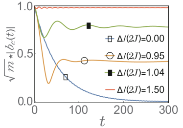
Figure 1: Time evolution of the magnitude of $b_{e}(t)$, the amplitude on the excited QEs with $m=3$. The time is in units of $1/(2J)$. Other parameters are $V/(2J)=0.08$ and $M=3$. Here and in all other figures, the plotted results are computed directly from our analytical results that have been also confirmed by numerical simulations based on the time-dependent Schrödinger equation.

To specifically and theoretically investigate the spontaneous emission dynamics, we start from the time-dependent Schrödinger equation

$$i\frac{\partial}{\partial t}\left|\psi\left(t\right)\right\rangle=H\left|\psi\left(t\right)\right\rangle\text{.}$$ (5)

The time-evolving state $\left|\psi\left(t\right)\right\rangle$ at time $t$ can be written as $\left|\psi\left(t\right)\right\rangle=\sum_{j}b_{j}(t)\left|e_{j},0\right\rangle+\sum_{k}C_{k}(t)\left|g,1_{k}\right\rangle$, where $b_{j}(t)$ ($j=1,2,...,M$) is the excitation amplitude for the $j$th QE in this sole type of QEs and $C_{k}(t)$ is the amplitude for the waveguide mode with wavenumber $k$. Applying Eq. (5), one obtains the following dynamical equations for the amplitudes

$$i\frac{\partial b_{j}\left(t\right)}{\partial t}=\Omega b_{j}\left(t\right)+\sum_{k}\frac{V}{\sqrt{N}}C_{k}\left(t\right)\text{,}$$ (6)

$$i\frac{\partial C_{k}\left(t\right)}{\partial t}=\omega_{k}C_{k}\left(t\right)+\sum_{j}\frac{V}{\sqrt{N}}b_{j}\left(t\right)\text{.}$$ (7)

To analytically solve these coupled dynamical equations, one may make use of the well-known Wigner-Weisskopf theory or Markovian theory by neglecting the contributions from any possible bound states. These two treatments can work well in the presence of one QE with the conditions $|\Omega-\omega_{c}|$ $\ll 2J$ and $V\ll 2J$, under which the bound-state trapping regime can be neglected [39]. However, such approximate treatment would not be able to capture a potential population trapping effect as mentioned above. To capture the impact of multiple QEs on population trapping, we must go beyond these approximations. To that end we take a Laplace transform for Eqs. (6) and (7) with $\tilde{b}_{j}(s)=\int_{0}^{\infty}b_{j}(t)e^{-st}dt$ and $\tilde{C}_{k}(s)=\int_{0}^{\infty}C_{k}(t)e^{-st}dt$. This yields

$$i\left[-b_{j}\left(0\right)+s\tilde{b}_{j}\left(s\right)\right]=\Omega\tilde{b}_{j}\left(s\right)+\sum_{k}\frac{V}{\sqrt{N}}\tilde{C}_{k}\left(s\right)\text{,}$$ (8)

$$i\left[-C_{k}\left(0\right)+s\tilde{C}_{k}\left(s\right)\right]=\omega_{k}\tilde{C}_{k}\left(s\right)+\sum_{j}\frac{V}{\sqrt{N}}\tilde{b}_{j}\left(s\right)\text{.}$$ (9)

Without loss of generality, we denote the initial excited QEs by index $j_{n}$, with $j_{n}$ going from $j_{1}$, $j_{2}$,…, to $j_{m}$ if there are initially $m$ QEs excited. All other QEs are in their ground states. Hence, the initial conditions in terms of the initial quantum amplitudes are: $b_{j_{1}}(0)=...=b_{j_{m}}(0)=1/\sqrt{m}$ ($m\leqslant M$), $b_{j}(0)=0$ ($j\neq j_{n}$), and $C_{k}(0)=0$. After some algebra, we obtain the expression of $\tilde{b}_{j_{1}}(s)=...=\tilde{b}_{j_{m}}(s)$ $\equiv$ $\tilde{b}_{e}(s)$ with $\tilde{b}_{e}(s)$ being

$$\tilde{b}_{e}\left(s\right)=i\frac{is-\Omega-\left(M-m\right)V^{2}F\left(s\right)}{\sqrt{m}\left(is-\Omega\right)\left[is-\Omega-MV^{2}F\left(s\right)\right]}\text{,}$$ (10)

where $F(s)=(1/N)\sum_{k}1/(is-\omega_{k})$. The time-evolving amplitudes for excited QEs can then be derived by use of the inverse Laplace transform $b_{j_{n}}(t)=(1/2\pi i)\int_{\sigma-i\infty}^{\sigma+i\infty}\tilde{b}_{j_{n}}(s)e^{st}ds$, with real number $\sigma$ being sufficiently large so that all the poles are on its left side. Note all the initially excited QEs have the same time-dependent amplitudes due to the chosen initial state. To calculate the integral here, the analytic properties of $\tilde{b}_{j_{n}}(s)$ are considered in the whole complex plane except a branch cut from $-i(2J+\omega_{c})$ to $i(2J-\omega_{c})$ along the imaginary axis. By using the residue theorem [46], we arrive at the exact expressions for $b_{j_{1}}(t)=...=b_{j_{m}}(t)$ $\equiv$ $b_{e}(t)$ with $b_{e}(t)$ being

$$b_{e}(t) =\sum_{n}\left.\frac{s+i\Omega+i\left(M-m\right)V^{2}F\left(s\right)}{\sqrt{m}\left[G_{1}\left(s\right)\right]^{\prime}}e^{st}\right|_{s=\varepsilon_{n}}$$

$$+\int_{-1}^{1}\frac{4\sqrt{m}V^{2}J^{2}\sqrt{1-y^{2}}e^{i2Jyt}}{L\left(y\right)+\pi M^{2}V^{4}}dy\text{,}$$ (11)

where

$$G_{1}(s)=(s+i\Omega)G_{0}(s)$$ (12)

with

$$G_{0}(s)=s+i\Omega+iMV^{2}F(s)$$ (13)

and $L(y)$ is defined as

$$L(y)=4\pi J^{2}(1-y^{2})(2Jy+\Omega)^{2}\text{.}$$ (14)

Here, $[G_{1}\left(s\right)]^{\prime}$ represents the derivative of $G_{1}(s)$ with respect to $s$. $\varepsilon_{n}$ is the roots of the equation $G_{1}(s)=0$. All these roots can be divided into two kinds. One is the solutions to the equation $G_{0}(s)=0$. This kind of roots are pure imaginary numbers, with their imaginary parts corresponding to minus eigenenergies of localized photon-QE bound states [39]. The other additional root is $s=-i\Omega$ and this root corresponds to the energy of dark states. In fact, according to the analysis using a complete basis expansion based on Green’s function method [34], the terms with $s$ being the solutions to the equation $G_{0}(s)=0$ in Eq. (13) comes from the contribution of system’s photon-QE bound states. The second line in Eq. (11) (which becomes zero in the limit of $t\rightarrow\infty$) arises from the contribution of system’s scattering states. When the number of initial excited QEs is equal to the total number of QEs, i.e., $m=M$, one can obtain $b_{e}(\infty)=\sum_{n}e^{st}/\{\sqrt{M}[G_{0}(s)]^{\prime}\}|_{t\rightarrow\infty,\text{ }s=\varepsilon_{n}^{\prime}}$ where $\varepsilon_{n}^{\prime}$ is solutions to the equation $G_{0}(s)=0$. The purely imaginary roots $\varepsilon_{n}^{\prime}$ reveal that the populations on the excited QEs are fractionally trapped when $t\rightarrow\infty$.

In Fig. 1, we plot the time dependence of $b_{e}(t)$ with $m=M=3$ and different detuning $\Delta=\Omega-\omega_{c}$. It can be seen that a larger fraction of the population is trapped at long time as the transition frequency $\Omega$ shifts away from the frequency $\omega_{c}$ of single resonator, and the spontaneous emission is almost totally suppressed when $\Omega$ is far away from the energy band. Exploring many examples, it is found that only under the condition $\sqrt{M}V\ll 2J$ and $|\Omega-\omega_{c}|$ $<J$ with which the first term in Eq. (11) can be ignored, the emission of QEs can be nearly complete and then display a basically exponential decay, with a slowly changing radiation rate as $\Omega$ varies from $\omega_{c}\pm J$ to $\omega_{c}$. For such a case, $\left|b_{e}(t)\right|^{2}$ can be approximately calculated as $\left|b_{e}(t)\right|^{2}\approx(1/M)e^{-\Gamma_{s}\left(\Delta\right)t}$, with a decay rate $\Gamma_{s}(\Delta)=2\pi MV^{2}D(\Delta)$, where $D(\Delta)$ is the density of states for the free-photon Hamiltonian. That is, only for such situations the spontaneous emission dynamics is best approximated by the Wigner-Weisskopf and Markovian approximate theory [47, 48]. Note also that under the condition of $\Delta=0$, $D(\Delta)$ gets its extremum, and $\Gamma_{s}(0)=MV^{2}/J$, which is $M$ times the radiation rate for the case of only one QE. This is precisely what a standard superradiance theory predicts.

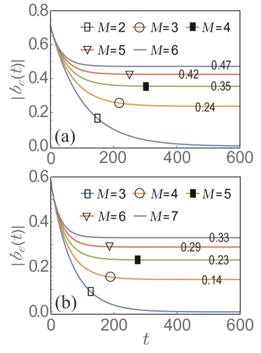
Figure 2: Time evolution of the magnitude of the excited-state amplitude $b_{e}(t)$ with different QE number $M$ for (a) $m=2$ and (b) $m=3$. Other parameters are $\Delta/(2J)=0$ and $V/(2J)=0.07$. Time is in units of $1/(2J)$.

Consider next what happens if the number of initially excited QEs is less than the total number of QEs, i.e., $m<M$. With the number $M\geqslant 2$, there are not only nonlocalized scattering states and localized photon-QE bound states, but also degenerate dark states with energy $E=\Omega$ [39, 40, 49]. These dark states have a specific property, namely, due to collective interference effects, these dark states allow only the QEs to be excited and so excitation amplitudes on the photon field modes are all zero. Therefore, now both such dark states and photon-QE bound states play a role in spontaneous emission dynamics. For the condition $\sqrt{M}V\ll 2J$ and $|\Omega-\omega_{c}|$ $<J$, with which the contributions from the photon-QE bound states are much smaller than that of the dark states, then the final values of $|b_{e}(t)|$ are found to depend only on the number $m$ of initial excited QEs and the total number $M$ of QEs. Specifically, for sufficiently long time (the second line of Eq. (11) can be dropped due to the highly oscillatory integral there) and upon neglecting the contributions from the roots of $G_{0}(s)=0$ that represent contributions from the photon-QE bound states, Eq. (11) reduces to

$$b_{e}(t) \approx \sum_{n}\left.\frac{s+i\Omega+i\left(M-m\right)V^{2}F\left(s\right)}{\sqrt{m}\left[G_{1}\left(s\right)\right]^{\prime}}e^{st}\right|_{s=\varepsilon_{n}}$$ (15)

$$\approx \left.\frac{s+i\Omega+i\left(M-m\right)V^{2}F\left(s\right)}{\sqrt{m}\left[G_{1}\left(s\right)\right]^{\prime}}e^{st}\right|_{s=-i\Omega}$$

$$= \frac{M-m}{\sqrt{m}M}e^{-i\Omega t}$$

This is one main result of this work.

In Fig. 2 (a), we plot our purely theoretical result of $|b_{e}(t)|$ assuming that two QEs are initially excited with different values of $M$, the total number of QEs in the system. As time lapsed is long enough, the final value of $|b_{e}(t)|$ during the emission dynamics is stabilized at $(M-2)/(\sqrt{2}M)$. Similarly, for the case where three QEs are initially excited, the amplitudes $b_{j_{1}}(t)=b_{j_{2}}(t)=b_{j_{3}}(t)$ $\equiv$ $b_{e}(t)$ at long time are found to stabilize at $|b_{e}(\infty)|$ $=(M-3)/(\sqrt{3}M)$ without further decay, as shown in Fig. 2 (b). Note again that the plotted results are computed directly from our analytical results derived above and have been also confirmed by our numerical results based on the time-dependent Schrödinger equation. These specific results hence have clearly illustrated our main theoretical prediction. For $m=1$, $\left|b_{e}(\infty)\right|$ comes back to the previous result already studied in the context of vacuum photonic bath, photonic crystal and coupled-resonator waveguide [40]. It is worth noting that Eq. (15) can also include the result with $m=M$. No trapping happens for this case and the initial energy of all QEs will be fully released, as also illustrated in Fig. 2 (a) and (b). Physically, this is because the initial excited states with $M=m$ are orthogonal to the dark states and as such, the presence of dark states is unable to saturate the spontaneous decay. From the view of prolonging the lifetime of QEs, we can see that under the condition $m\ll M$, our theory above predicts that the spontaneous emission of the QEs will be greatly suppressed.

IV Dynamics and trapping law with two types of QEs

We now investigate the properties of dynamics in the waveguide system with two different types of QEs indexed by $A$ and $B$. Unlike the case with one sole type of QEs where there are always two photon-QE bound states, the energy-level structure of the system with two type of QEs can undergo certain transitions when some system parameters change [39], such as the QE numbers $M_{A}$ and $M_{B}$ or the coupling strengths $V_{A}$ and $V_{B}$. When overall only one QE is initially excited (without loss of generality, assuming that the excited QE belongs to type $A$), then previously it was found that the asymptotic value of the magnitude of the quantum amplitude of the QE is given by $1-1/M_{A}$ [39]. Encouraged by our results from the previous section, here we wish to examine if there is some similar trapping law if more than one QEs, but still belonging to the same type, are initially excited. One main complication in answering this question is that the two types of QEs can interact strongly with each other through the waveguide system. As such, to observe an interesting trapping law it is necessary to find under what theoretical conditions the decay dynamics can still exhibit some trapping law. A violation of the trapping law sought after here will give us strong indication of the interplay between different types of QEs.

Let us now proceed with our theoretical framework. In the single excitation subspace, the time-evolving state at time $t$ can be written as

$$\left|\varphi\left(t\right)\right\rangle=\sum_{i}\sum_{j}b_{j}^{i}\left(t\right)\left|e_{j}^{i},0\right\rangle+\sum_{k}C_{k}\left(t\right)\left|g,1_{k}\right\rangle\text{,}$$ (16)

where $b_{j}^{i}(t)$ ($i=A,B$) is the excitation amplitude of the system’s state for the $j$th QE of type $i$, with no photon in the waveguide. $C_{k}(t)$ is the amplitude for the state that all QEs are in their ground states and there is a photon with wavenumber $k$. Plugging $\left|\varphi(t)\right\rangle$ into the Schrödinger equation $i\partial\left|\varphi\left(t\right)\right\rangle/\partial t=H\left|\varphi\left(t\right)\right\rangle$, one can obtain the following coupled equations for $b_{j}^{i}\left(t\right)$ and $C_{k}\left(t\right)$

$$i\frac{\partial}{\partial t}b_{j}^{i}\left(t\right)=\Omega_{i}b_{j}^{i}\left(t\right)+\sum_{k}\frac{V_{i}}{\sqrt{N}}C_{k}\left(t\right)\text{,}$$ (17)

$$i\frac{\partial}{\partial t}C_{k}\left(t\right)=\omega_{k}C_{k}\left(t\right)+\sum_{i}\sum_{j}\frac{V_{i}}{\sqrt{N}}b_{j}^{i}\left(t\right)\text{.}$$ (18)

Similar to the steps in the case of one type of QEs, one can take a Laplace transform for Eqs. (17) and (18) with $\tilde{b}_{j}^{i}(s)=\int_{0}^{\infty}b_{j}^{i}(t)e^{-st}dt$ and $\tilde{C}_{k}(s)=\int_{0}^{\infty}C_{k}(t)e^{-st}dt$, which leads to

$$i\left[-b_{j}^{i}\left(0\right)+s\tilde{b}_{j}^{i}\left(s\right)\right]=\Omega_{i}\tilde{b}_{j}^{i}\left(s\right)+\sum_{k}\frac{V_{i}}{\sqrt{N}}\tilde{C}_{k}\left(s\right)\text{,}$$ (19)

$$i\left[-C_{k}\left(0\right)+s\tilde{C}_{k}\left(s\right)\right]=\omega_{k}\tilde{C}_{k}\left(s\right)+\sum_{i}\sum_{j}\frac{V_{i}}{\sqrt{N}}\tilde{b}_{j}^{i}\left(s\right)\text{.}$$ (20)

Let us now assume that initially only one type of QEs are excited and without loss of generality, the excited QEs denoted by index $j_{n}$ are assumed to be of type $A$. We further assume that in total $m_{A}$ QEs of type $A$ are initially excited and all other QEs are in their ground state, with amplitudes $b_{j_{1}}^{A}(0)=...=b_{j_{m_{A}}}^{A}(0)=1/\sqrt{m_{A}}$ ($m_{A}\leqslant M_{A}$), $b_{j}^{A}(0)=0$ ($j\neq j_{n}$), $b_{j}^{B}(0)=0$ and $C_{k}(0)=0$. After some necessary algebraic operations with Eq. (19) and (20), one can arrive at the expression of $\tilde{b}_{j_{1}}^{A}(s)=...=\tilde{b}_{j_{m_{A}}}^{A}(s)$ $\equiv$ $\tilde{b}_{e}^{A}(s)$ with $\tilde{b}_{e}^{A}(s)$ being

$$\tilde{b}_{e}^{A}\left(s\right) =i\frac{K_{A}\left(s\right)K_{B}\left(s\right)+m_{A}V_{A}^{2}F\left(s\right)K_{B}\left(s\right)}{\sqrt{m_{A}}\left(is-\Omega_{A}\right)Y\left(s\right)}$$

$$-i\frac{\left(M_{A}-m_{A}\right)M_{B}\left[V_{A}V_{B}F\left(s\right)\right]^{2}}{\sqrt{m_{A}}\left(is-\Omega_{A}\right)Y\left(s\right)}$$ (21)

where

$$K_{i}(s)=is-\Omega_{i}-M_{i}V_{i}^{2}F(s)\text{,}$$ (22)

and

$$Y(s)=K_{A}(s)K_{B}(s)-M_{A}M_{B}[V_{A}V_{B}F(s)]^{2}\text{.}$$ (23)

Just like what was done in the previous section, the time dependence of the excited QEs can be calculated by the inverse Laplace transform. Because $\tilde{b}_{j_{n}}^{A}(s)$ is an analytic function in the whole complex plane except a branch cut from $-i(2J+\omega_{c})$ to $i(2J-\omega_{c})$ along the imaginary axis, the exact expressions of the excited amplitudes $b_{j_{1}}^{A}(t)=...=b_{j_{m_{A}}}^{A}(t)$ $\equiv$ $b_{e}^{A}(t)$ can be acquired by using the residue theorem [46] and $b_{e}^{A}(t)$ is obtained as

$$b_{e}^{A}(t) =\left.\frac{\left(M_{A}-m_{A}\right)}{\sqrt{m_{A}}M_{A}}e^{st}\right|_{s=-i\Omega_{A}}$$

$$-\sum_{n}\left.\frac{\left(s+i\Omega_{B}\right)m_{A}V_{A}^{2}F\left(s\right)}{\sqrt{m_{A}}\left(is-\Omega_{A}\right)\left[G_{2}\left(s\right)\right]^{\prime}}e^{st}\right|_{s=\tilde{\varepsilon}_{n}}$$

$$+\sum_{\alpha=\pm 1}\int_{-1}^{1}\frac{J\left(2Jy+\Omega_{B}\right)m_{A}V_{A}^{2}f\left(y\right)e^{i2Jyt}}{\pi\sqrt{m_{A}}\left(2Jy+\Omega_{A}\right)Z_{\alpha}\left(y\right)}dy$$ (24)

where

$$G_{2}(s) = (is-\Omega_{A})(is-\Omega_{B})-(is-\Omega_{A})M_{B}V_{B}^{2}F(s)$$ (25)

$$-(is-\Omega_{B})M_{A}V_{A}^{2}F(s)$$

and $\tilde{\varepsilon}_{n}$ is the roots of the equation $G_{2}(s)=0$. We stress that $G_{2}(-iE)=0$ can be used to determine the eigenenergies $E$ of localized photon-QE bound states [39]. Because $G_{2}(s)$ involves physical properties of both types of QEs, in general one anticipates that photon-QE bound states here can lead to rather complicated population trapping behavior [35]. As to the third term from the contribution of the scattering states in Eq. (24), it contains functions $f(y)$ and $Z_{\pm}(y)$ defined as $f(y)=1/(2J\sqrt{1-y^{2}})$ and $Z_{\pm}(y)=(2Jy+\Omega_{A})(2Jy+\Omega_{B})\pm i[(2Jy+\Omega_{A})M_{B}V_{B}^{2}+(2Jy+\Omega_{B})M_{A}V_{A}^{2}]f(y)$. As expected, we also see a highly oscillatory factor $e^{i2Jyt}$ in the long time limit, thus killing the third term for long time dynamics.

Despite the complicated contributions from the photon-QE bound states involving two types of QEs, what we learned from the previous section is that there are still a wide parameter regime where we may focus on the contributions of the dark state only with the bound-state contributions being negligible. That is, if the magnitude of $(s+i\Omega_{B})m_{A}V_{A}^{2}F(s)/\{\sqrt{m_{A}}(is-\Omega_{A})[G_{2}(s)]^{\prime}\}|_{s=\tilde{\varepsilon}_{n}}$ is sufficiently small, which may be satisfied, e.g., under the condition $V_{A}\ll 2J$, the asymptotic amplitude $b_{e}^{A}(t)$ can be easily identified as well, namely,

$$\left|b_{e}^{A}(\infty)\right|=\frac{M_{A}-m_{A}}{\sqrt{m_{A}}M_{A}}\text{.}$$ (26)

Interestingly, one sees that $|b_{e}^{A}(\infty)|$ is only related with the number $m_{A}$ of initially excited emitters and the total number $M_{A}$ of emitters of type $A$, thus still exhibiting a simple trapping law of emission dynamics. In Fig. 3 (a), we plot the theoretical time evolution of $|b_{e}^{A}((t)|$ with different numbers $m_{A}$ of initially excited QEs for $M_{A}=5$. It is seen that $|b_{e}^{A}((t)|$ asymptotically approaches $(M_{A}-m_{A})/(\sqrt{m_{A}}M_{A})$. On top of this remarkably simple behavior, $|b_{e}^{A}((t)|$ is seen to be stabilized or trapped, but with some small-amplitude oscillation behavior. This oscillation behavior can be traced back to the contribution from the above-neglected photon-QE bound states, associated with the second term in Eq. (24). One would imagine that if the coupling strength $V_{A}$ is tuned to be smaller so that the theoretical condition $(s+i\Omega_{B})m_{A}V_{A}^{2}F(s)/\{\sqrt{m_{A}}(is-\Omega_{A})[G_{2}(s)]^{\prime}\}|_{s=\tilde{\varepsilon}_{n}}\ll 1$ is better satisfied, then the said oscillations will become less obvious.

As a final interesting check to motivate future studies, let us now investigate the emission dynamics via $|b_{e}^{A}((t)|$ in Fig. 3 (b) with the condition $V_{B}/(2J)=0.6$. Under this stronger coupling condition from type-B emitters, the role of the second term in Eq. (24) or the contributions from the photon-bound states can no longer be neglected. Indeed, as we see from the actual results, the previously identified trapping law is completely broken due to the strong interplay between type-A and type-B QEs.

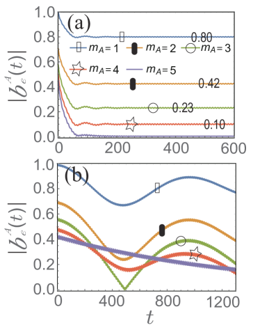
Figure 3: Time evolution of the magnitude of the excited-state amplitude $b_{e}^{A}(t)$ with different number $m_{A}$ of initially excited QEs in type $A$ for (a) $V_{B}/(2J)=0.1$ and (b) $V_{B}/(2J)=0.6$. Other parameters are: $\Delta_{A}/(2J)=0.3$, $\Delta_{B}/(2J)=0.2$, $V_{A}/(2J)=0.1$, $M_{A}=5$ and $M_{B}=2$. The time is in units of $1/(2J)$.

We conclude this section with more qualitative discussions. Due to the presence of two different types of identical QEs, there are two types of degenerate dark states. Dark states due to type-A QEs have energy $E=\Omega_{A}$ whereas the other type of dark states has energy $E=\Omega_{B}$. However, because of the orthogonality of these two different types of dark states, only the dark states with $E=\Omega_{A}$ makes a difference to the emission dynamics if only type-A QEs are initially excited. Nevertheless, this simple picture is valid only if the impact of population trapping from the photon-QE bound states is negligible. In the parameter regime where the population trapping law still persists, it is seen that under the condition $m_{A}\ll M_{A}$, the spontaneous emissions from type-A QEs can be greatly inhibited by the presence of dark states.

V Discussion and conclusion

We have studied the single-photon collective emission dynamics in a one-dimensional waveguide array system. Assuming that the size of the ensemble of QEs is much smaller than the wavelength of the radiation field, we have neglected the spatial difference between the QEs. Our model system supports stable subradiant states composed of dark states that preserve the collective excitation of QEs. Unlike the trapping regime caused by the photon-QE bound states, we find that the long-time emission dynamics of the subradiant states can be characterized by a unified population trapping law. This trapping law has nothing to do with the dispersion of the bosonic bath or the coupling strength between the photon field and the QEs. Instead, it is only related with the number of initially excited QEs and the total number of QEs. When more than one type of QEs are present, a similar trapping law persists if the effect of the composite photon-QE bound state can be neglected.

Finally, we discuss the possible experimental platform consisting of transmon qubits and coupled superconducting resonators which have been realized in recent years [41, 42, 43, 50, 51, 52]. In such systems, the hopping energy $J\approx 20$-$730(2\pi)$ MHz. The qubit-resonator coupling strength $V$ is in the range of $5$-$300(2\pi)$ MHz. Thus the key parameter $V/(2J)\ll 1$ can be achieved with the existing technology. The frequencies of transmon qubits can be controlled in the range of $1$-$10(2\pi)$ GHz [5, 53], which is similar to the range of the resonance frequency of each resonator, hence being sufficient to yield small detuning $\Delta$ or near-resonance conditions considered in this work.

References

- [1] D. F. Walls and G. J. Milburn, Quantum Optics (Springer Science & Business Media, 2007).
- [2] D. E. Chang, A. S. Sorensen, E. A. Demler, and M. D. Lukin, A single-photon transistor using nanoscale surface plasmons, Nat. Phys. 3, 807 (2007).
- [3] M. Rycenga, C. M. Cobley, J. Zeng, W. Li, C. H. Moran, Q. Zhang, D. Qin, and Y. Xia, Controlling the synthesis and assembly of silver nanostructures for plasmonic applications, Chem. Rev. 111, 3669 (2011).
- [4] P. Lodahl, S. Mahmoodian, and S. Stobbe, Interfacing single photons and single quantum dots with photonic nanostructures, Rev. Mod. Phys. 87, 347 (2015).
- [5] A. Blais, A. L. Grimsmo, S. M. Girvin, and A. Wallraff, Circuit quantum electrodynamics, Rev. Mod. Phys. 93, 025005 (2021).
- [6] M. S. Tame, K. R. McEnery, S. K. Özdemir, J. Lee, S. A. Maier, and M. S. Kim, Quantum plasmonics, Nat Phys 9, 329 (2013).
- [7] H. Zheng and H. U. Baranger, Persistent quantum beats and long-distance entanglement from waveguide-mediated interactions, Phys. Rev. Lett. 110, 113601 (2013).
- [8] G. Z. Song, J. L. Guo, W. Nie, L. C. Kwek, and G. L. Long, Optical properties of a waveguide-mediated chain of randomly positioned atoms, Opt. Express 29, 1903 (2021).
- [9] J. Petersen, J. Volz, and A. Rauschenbeutel, Chiral nanophotonic waveguide interface based on spin-orbit interaction of light, Science 346, 67 (2014).
- [10] P. Lodahl, S. Mahmoodian, S. Stobbe, P. Schneeweiss, J. Volz, A. Rauschenbeutel, H. Pichler, P. Zoller, Chiral quantum optics, Nature 541, 473 (2017).
- [11] E. Sánchez-Burillo, L. Martín-Moreno, J. J. Garc ía-Ripoll, and D. Zueco, Single photons by quenching the vacuum, Phys. Rev. Lett. 123, 013601 (2019).
- [12] Z. H. Wang, T. Jaako, P. Kirton, and P. Rabl, Supercorrelated radiance in nonlinear photonic waveguides, Phys. Rev. Lett. 124, 213601 (2020).
- [13] F. W. Cummings and A. Dorri, Exact solution for spontaneous emission in the presence of N atoms, Phys. Rev. A 28, 2282 (1983).
- [14] F. W. Cummings, Spontaneous emission from a single two-level atom in the presence of N initially unexcited identical atoms, Phys. Rev. A 33, 1683 (1986).
- [15] G. Benivegna and A. Messina, Physical origin of the radiation suppression in the spontaneous emission of an excited atom in the presence of N-1 atoms, Phys. Lett. A 126, 249 (1988).
- [16] V. Buzek, Dynamics of an excited two-level atom in the presence of N-1 unexcited atoms in the free space, Phys. Rev. A 39, 2232 (1989).
- [17] V. Buzek, G. Drobny, M. G. Kim, M. Havukainen, and P. L. Knight, Numerical simulations of atomic decay in cavities and material media, Phys. Rev. A 60, 582 (1999).
- [18] R. H. Dicke, Coherence in spontaneous radiation processes, Phys. Rev. 93, 99 (1954).
- [19] M. Gross, and S. Haroche, Superradiance: An essay on the theory of collective spontaneous emission, Phys. Rep. 93, 301 (1982).
- [20] M. D. Eisaman, L. Childress, A. André, F. Massou, A. S. Zibrov, and M. D. Lukin, Shaping quantum pulses of light via coherent atomic memory, Phys. Rev. Lett. 93, 233602 (2004).
- [21] A. I. Lvovsky, B. C. Sanders, and W. Tittel, Optical quantum memory, Nature Photonics 3, 706 (2009).
- [22] A. Nicolas, L. Veissier, L. Giner, E. Giacobino, D. Maxein, and J. Laurat, A quantum memory for orbital angular momentum photonic qubits, Nature Photonics 8, 234 (2014).
- [23] A. Kuzmich, W. P. Bowen, A. D. Boozer, A. Boca, C. W. Chou, L.-M. Duan, and H. J. Kimble, Generation of nonclassical photon pairs for scalable quantum communication with atomic ensembles, Nature 423 , 731 (2003).
- [24] D. N. Matsukevich and A. Kuzmich, Quantum state transfer between matter and light, Science 306, 663 (2004).
- [25] D. Porras and J. I. Cirac, Collective generation of quantum states of light by entangled atoms, Phys. Rev. A 78, 053816 (2008).
- [26] J.-W. Pan, Z.-B. Chen, C.-Y. Lu, H. Weinfurter, A. Zeilinger, and M. Zukowski, Multiphoton entanglement and interferometry, Rev. Mod. Phys. 84, 777 (2012).
- [27] A. W. Eddins, C. C. Beedle, D. N. Hendrickson, and J. R. Friedman, Collective coupling of a macroscopic number of single-molecule magnets with a microwave cavity mode, Phys. Rev. Lett. 112, 120501 (2014).
- [28] P. Y. Wen, K.-T. Lin, A. Kockum, B. Suri, H. Ian, J. C. Chen, S. Y. Mao, C. C. Chiu, P. Delsing, F. Nori, G.-D. Lin, and I.-C. Hoi, Large collective Lamb shift of two distant superconducting artificial atoms, Phys. Rev. Lett. 123, 233602 (2019).
- [29] F. Lombardo, F. Ciccarello, and G. M. Palma, Photon localization versus population trapping in a coupled-cavity array, Phys. Rev. A 89, 053826 (2014).
- [30] G. Calajó, F. Ciccarello, D. Chang, and P. Rabl, Atom-field dressed states in slow-light waveguide QED, Phys. Rev. A 93, 033833 (2016).
- [31] Y.-J. Song and L. Qiao, Controlling single-photon scattering in a rectangular waveguide by a V-type three-level emitter, Opt. Express 28, 37639 (2020).
- [32] E. Sánchez-Burillo, D. Zueco, L. Martín-Moreno, and J. J. García-Ripoll, Dynamical signatures of bound states in waveguide QED, Phys. Rev. A 96, 023831 (2017).
- [33] L. Qiao, Single-photon transport through a waveguide coupling to a quadratic optomechanical system, Phys. Rev. A 96, 013860 (2017).
- [34] L. Qiao, Y. J. Song, and C. P. Sun, Quantum phase transition and interference trapping of populations in a coupled-resonator waveguide, Phys. Rev. A 100, 013825 (2019).
- [35] S. John and T. Quang, Spontaneous emission near the edge of a photonic band gap, Phys. Rev. A 50, 1764 (1994).
- [36] A. G. Kofman, G. Kurizki, and B. Sherman, Spontaneous and induced atomic decay in photonic band structures, J. Mod. Opt. 41, 353 (1994).
- [37] K. Sakoda, Optical Properties of Photonic Crystals (Springer-Verlag, Berlin Heidelberg, 2001).
- [38] S. John and J. Wang, Quantum electrodynamics near a photonic band gap: Photon bound states and dressed atoms, Phys. Rev. Lett. 64, 2418 (1990).
- [39] L. Qiao and C. P. Sun, Atom-photon bound states and non-markovian cooperative dynamics in coupled-resonator waveguides, Phys. Rev. A 100, 063806 (2019).
- [40] L. Qiao and C. P. Sun, Universal trapping law induced by an atomic cloud in single-photon cooperative dynamics, Phys. Rev. A 101 , 063831 (2020).
- [41] M. Fitzpatrick, N. M. Sundaresan, A. C. Y. Li, J. Koch, and A. A. Houck, Observation of a dissipative phase transition in a one-dimensional circuit QED lattice, Phys. Rev. X 7, 011016 (2017).
- [42] N. M. Sundaresan, R. Lundgren, G. Zhu, A. V. Gorshkov, and A. A. Houck, Interacting qubit-photon bound states with superconducting circuits, Phys. Rev. X 9, 011021 (2019).
- [43] V. S. Ferreira, J. Banker, A. Sipahigil, M. H. Matheny, A. J. Keller, E. Kim, M. Mirhosseini, and O. Painter, Collapse and revival of an artificial atom coupled to a structured photonic reservoir, Phys. Rev. X 11, 041043 (2021).
- [44] M. Notomi, E. Kuramochi, and T. Tanabe, Large-scale arrays of ultrahigh-Q coupled nanocavities, Nat. Photon. 2, 741 (2008).
- [45] N. Meher and S. Sivakumar, A review on quantum information processing in cavities, Eur. Phys. J. Plus 137, 985 (2022).
- [46] K. F. Riley, M. P. Hobson, and S. J. Bence, Mathematical Methods for Physics and Engineering, 3rd ed. (Cambridge University Press, Cambridge, 2006).
- [47] M. O. Scully and M. S. Zubairy, Quantum Optics (Cambridge University Press, Cambridge, UK, 1997).
- [48] L. Qiao and J. Gong, Coherent control of collective spontaneous emission through self-interference, Phys. Rev. Lett. 129 , 093602 (2022).
- [49] C. P. Sun, Y. Li, and X. F. Liu, Quasi-spin-wave quantum memories with a dynamical symmetry, Phys. Rev. Lett. 91, 147903 (2003).
- [50] D. C. McKay, R. Naik, P. Reinhold, L. S. Bishop, and D. I. Schuster, High-Contrast Qubit Interactions Using Multimode Cavity QED , Phys. Rev. Lett. 114, 080501 (2015).
- [51] M. Scigliuzzo, G. Calajò, F. Ciccarello, D. P. Lozano, A. Bengtsson, P. Scarlino, A. Wallraff, D. Chang, P. Delsing, and S. Gasparinetti. Controlling Atom-Photon Bound States in an Array of Josephson-Junction Resonators, Phys. Rev. X 12, 031036, (2022).
- [52] E. Kim, X. Zhang, V. S. Ferreira, J. Banker, J. K. Iverson, A. Sipahigil, M. Bello, A. González-Tudela, M. Mirhosseini, and O. Painter, Quantum Electrodynamics in a Topological Waveguide, Phys. Rev. X 11, 011015 (2021).
- [53] X. Gu, A. F. Kockum, A. Miranowicz, Y. X. Liu, and F. Nori, Microwave photonics with superconducting quantum circuits, Phys. Rep. 718–719, 1 (2017).