Exploring Shallow-Depth Boson Sampling: Towards Scalable Quantum Supremacy

Abstract

Boson sampling is a sampling task proven to be hard to simulate efficiently using classical computers under plausible assumptions, which makes it an appealing candidate for quantum supremacy. However, due to a large noise rate for near-term quantum devices, it is still unclear whether those noisy devices maintain the quantum advantage for much larger quantum systems. Since the noise rate typically grows with the circuit depth, an alternative is to find evidence of simulation hardness at the shallow-depth quantum circuit. To find the evidence, one way is to identify the minimum depth required for the average-case hardness of approximating output probabilities, which is considered a necessary condition for the state-of-the-art technique to prove the simulation hardness of boson sampling. In this work, we analyze the output probability distribution of shallow-depth boson sampling for Fock-states and Gaussian states, and examine the limitation of the average-case hardness argument at this shallow-depth regime for geometrically local architectures. We propose a shallow-depth linear optical circuit architecture that can overcome the problems associated with geometrically local architectures. Our numerical results suggest that this architecture demonstrates possibilities of average-case hardness properties in a shallow-depth regime, through its resemblance to the global Haar-random boson sampling circuit. This result implies that the corresponding architecture has the potential to be utilized for scalable quantum supremacy with its shallow-depth boson sampling.

I Introduction

We live in an exciting era with the emergence of noisy intermediate-scale quantum (NISQ) devices [1]. Those NISQ devices are expected to be able to outperform classical computers in some computational tasks, which refers to quantum advantage or quantum supremacy. Various computational problems are proposed to be a candidate for demonstrating quantum advantage with NISQ devices, and the prominent candidates at the present time are boson sampling (BS) [2, 3, 4] and random circuit sampling (RCS) [5, 6]; both denote sampling problems from the random quantum circuit instances but in different systems. They have been complexity-theoretically proven to be hard to efficiently simulate with classical computers under plausible assumptions. Ever since the theoretical foundation [2, 5, 3, 4], there have been plenty of experimental results claiming the first realization of quantum advantage with BS [7, 8, 9, 10] and RCS [11, 6, 12, 13].

However, it is still unclear whether the quantum advantage can be maintained for larger quantum systems, and beyond that, for the asymptotic limits as system size scales. The major obstacle to the scalability of the quantum advantage is the uncorrected noise on near-term quantum devices, which suppresses the quantumness and may eventually allow efficient classical simulation. In particular, as the noise rate typically grows with circuit depth, the circuit depth should not be too large to accomplish the hardness of classical simulation for noisy devices. Otherwise, the accumulated noise induced by a large-depth circuit may result in the loss of quantumness and classical intractability. On the other hand, the circuit depth should also be large enough to achieve the simulation hardness, as a shallow depth circuit leads to the weakly entangled quantum state, which is often efficiently simulable by classical algorithms [14, 15, 16, 17, 18, 19, 20]. Therefore, to attain the scalable quantum advantage with noisy quantum devices, it is necessary to identify an appropriate regime, where the depth is large enough to generate the quantumness and not too large to lose the classical intractability by the uncorrected noise.

To be more specific about the effect of noise on the complexity, there are many results proposing the possibilities of the efficient classical simulation of noisy BS and RCS as system size scales, hindering the scalability of the quantum advantage. For the RCS case, Refs. [21, 22, 23, 24, 25] suggested a probability distribution of most quantum circuits of super-logarithmic depth with a constant level of noise (depolarizing, Pauli, etc) applied for each unit depth converges to a uniform distribution. Similarly, for the BS case, there have been many results [26, 27, 28, 29, 30, 31, 32, 33] about efficient classical algorithms to simulate noisy BS, with various noise models, such as photon loss and partial distinguishability of photons. Those results suggest that noisy BS can be efficiently simulated if the noise rate is sufficiently large.

As an example, for photon loss, if the output photon numbers are less than $\mathcal{O}(\sqrt{N})$ for input photon number $N$, BS becomes efficiently simulatable within a constant total variation distance [34, 35, 36]. Since the output photon number is given by $N_{\text{out}}=NT^{D}$ for circuit depth $D$ and a transmission rate $T$ applied at each depth, it implies the easiness of classical simulation for superlogarithmic circuit depth unless the transmission rate per depth $T$ increases with system size, which is typically unrealistic. Therefore, according to the above discussions, circuit depth superlogarithmic with system size would possibly rule out the scalable demonstration of the quantum advantage [35].

The above example clearly shows that as circuit depth grows, more noises are accumulated in the system. Hence, an obvious way to suppress the effect of loss is to consider shallow-depth circuits and investigate if we can still maintain hardness in shallow-depth circuits. A crucial factor in proving the hardness of approximate sampling, which represents noisy BS, using the state-of-the-art technique is the average-case hardness of output probability approximation within a certain additive imprecision (viz., on average over random circuit instances) [2, 5, 3, 4, 37, 38, 39]. One evidence often cited as the average-case hardness, but not sufficient, is an anti-concentration property [2, 5, 40, 41, 42, 43], which is a measure of the flatness of probability distribution. For the RCS case, recent results found that the probability distribution of logarithm depth random quantum circuit is anti-concentrated [44, 43], but poorly anti-concentrated for sub-logarithm depth [25]. Those results suggested hope that log-depth RCS may have the average-case hardness property and thus may be a suitable candidate for realizing scalable quantum advantage even with noisy devices. However, more recently, Ref. [45] presented a polynomial-time classical simulation of noisy log-depth RCS with a constant level of noise per depth using the anti-concentration property, deflating the hope.

Meanwhile, for the BS case, output probability distributions and their average-case approximation hardness for shallow-depth BS have been less studied compared to the RCS case, to the best of our knowledge. There have been some results about efficient classical algorithms to simulate shallow-depth BS, but they can be applied only in particular circumstances. Specifically, Ref. [19] suggested a classical algorithm that can simulate 1$d$ logarithm depth BS efficiently. Also, Refs. [18, 20] proposed classical algorithms which can efficiently simulate BS for the higher dimensional local circuits but on condition that input sources are well-separated, under a certain depth such that the well-separated input sources do not correlate much with each other. Although those algorithms can clarify the easiness of simulating shallow-depth BS for specific cases, it remains an open question whether there can be the average-case hardness of shallow-depth BS with more general setups, e.g., allowing different circuit architectures, circuit ensembles, and input configurations. Hence, the motivation of our work is to investigate the possibility of shallow-depth BS that achieves simulation hardness, by analyzing the behavior of output probability distributions in low-depth regimes for general setups.

In this work, we find that the probability distribution is too concentrated to achieve the average-case hardness of probability approximation for local linear-optical circuits under a certain polynomial depth, regardless of circuit ensembles and input configurations, both for Fock-state BS (FBS) and Gaussian BS (GBS) schemes. We prove that from the structure of the local parallel circuit architecture, a typical way to build a random linear-optical network using geometrically local gates, most of the outcomes are forbidden at the shallow depth regime, i.e., have zero probability, regardless of circuit ensembles. Besides, if we employ local random circuit ensembles, their diffusive properties make probability distribution concentrated even inside the permitted outcomes, requiring additional circuit depth to get out of the concentrated regime.

Following the above examination, we propose a linear-optical circuit architecture that can resolve the above issues within logarithm depth, using geometrically non-local gates. We numerically examine that the corresponding circuit architecture with each gate drawn from the local random unitary can well imitate the behavior of the global Haar random unitary, the requirement to achieve evidence of the average-case hardness, in a shallow depth regime. Specifically, output probability distribution and entanglement generation of the above random circuit setup show fast convergence toward those of the global Haar random circuit with increasing circuit depth. Those results highlight that the corresponding circuit architecture shows a potential to achieve the average-case hardness in the shallow depth regime and be utilized as an architecture for scalable quantum advantage with BS.

The paper is organized as follows. In Sec. II, we begin with a brief introduction of the average-case hardness of approximating output probabilities of BS and discuss the possible issues that may arise when we lower the depth. In Sec. III, we present problems of geometrically local architectures, which hinder the anti-concentration and thus do not allow the average-case hardness below a certain polynomial depth. In Sec. IV, we propose a geometrically non-local circuit architecture that can resolve the problems we addressed within logarithm depth. We numerically examine the probability distribution and entanglement of the circuit for various system sizes. In Sec. V, we conclude with a few remarks.

II Average-case hardness of output probability approximation

We first briefly recall the average-case hardness of BS and investigate if a similar hardness still holds in the low-depth regime, examining potential issues that may arise when we lower the depth. There are two major schemes of BS, which are FBS and GBS, and we consider the average-case hardness of FBS first. The output probability of FBS is expressed as permanent, which is worst-case #P-hard to compute [2, 46]. To achieve the average-case #P-hardness of the output probability approximation, the implementation of random circuit instances is required. Specifically, the current proof technique requires that unitary matrices corresponding to the random circuits must be drawn from Haar measure on U($M$), where $M$ corresponds to the total mode number. Under some plausible assumptions (see [2] for more details), approximating most of the output probabilities of FBS on average over random linear-optical circuits is #P-hard, which can be represented as follows.

Conjecture 1.

For mode number $M$ and photon number $N$, approximating most output probabilities of most linear-optical circuits within additive error $\operatorname*{\text{poly}}(N)^{-1}\frac{N!}{M^{N}}$ is #P-hard.

Also, a similar argument is established for GBS in [3, 4], whose output probability is now expressed as hafnian, which is at least as hard as permanent to compute. Those results suggest that for fixed output photon number $N$, approximating most of the output probabilities of GBS on average over random linear-optical circuits is #P-hard, under plausible assumptions.

Accordingly, implementing $M$-mode random linear optical circuits corresponding to $M$-dimensional Haar random unitary matrices is necessary to find evidence of the average-case hardness of BS using the current techniques (both for FBS and GBS schemes). However, the exact implementation of Haar random unitary matrices requires at least polynomially large circuit depth (e.g., results in Ref. [47]). More precisely, as the space of $M$ dimensional unitary matrices is determined by $M^{2}$ independent parameters [48], $\Omega(M^{2})$ number of local random unitary gates are required to implement global Haar random unitary, which can only be accomplished by $\Omega(M)$ circuit depth.

One way to find evidence of the average-case hardness of approximating output probabilities in the low-depth regime, as we discussed in the previous section, is by investigating the anti-concentration property of the corresponding output probability distribution. Although anti-concentration solely does not guarantee the hardness of output probability estimation, at least it can propose the minimum depth required for the average-case hardness, i.e., necessary but not sufficient condition. Specifically, when the output probability distribution is concentrated such that most of the output probabilities are very close to zero and easy to approximate within additive error by a trivial algorithm that always outputs the value “0”, there is no average-case hardness of approximating output probabilities. Therefore, if the output probability of BS below a certain depth is poorly anti-concentrated as described above, the corresponding depth suggests a prerequisite for the average-case hardness of output probability approximation, as we cannot achieve the average-case hardness below the depth.

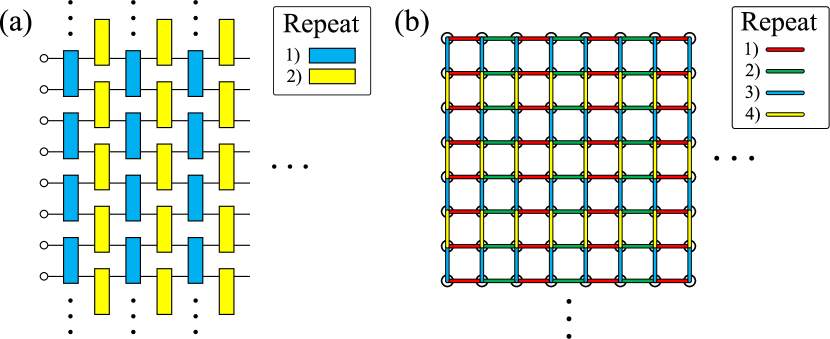
Figure 1: Schematics of (a) 1$d$ and (b) 2$d$ local parallel circuit. Unitary gates with the same colors are applied in parallel, and the sequence is $2$ steps of the parallel application of local gates for each dimension. Here, such application of gates with the same color implies the unit depth.

III Limitations of geometrically local architectures

We consider an $M$-mode linear optical circuit characterized by unitary operator $\hat{\mathcal{U}}$. After the evolution, input mode operators of the system are linearly transformed by a unitary matrix $U$ defined as

$$\hat{a}_{i}\Longrightarrow\hat{\mathcal{U}}^{{\dagger}}\hat{a}_{i}\hat{\mathcal{U}}=\sum_{j=1}^{M}U_{ij}\hat{a}_{j}$$ (1)

The probability of each outcome of BS is represented by a function of the unitary matrix $U$, which corresponds to permanent and hafnian for FBS and GBS, respectively.

A typical way to construct an $M$-mode random linear-optical network is a local parallel circuit architecture, a parallel array of geometrically local beam splitters that can interact with only nearest-neighbor modes [49]. The corresponding circuit architecture has often been used both for theoretical [50, 20, 47] and experimental [51, 7, 8, 52] studies, as a building block for random linear-optical circuits. There are schematics of the 1$d$ and 2$d$ local parallel circuits in Fig. 1, and we can easily generalize those circuits to a $d$-dimensional local parallel circuit. More formally, the $d$-dimensional local parallel circuit with depth $D$ consists of $D/2d$ rounds, where a single round consists of $2d$ steps, $2$ steps of the parallel application of local gates for each dimension. Here and throughout, we emphasize that a unit depth in our work refers to a single step of parallel application of gates at a fixed dimension, to avoid any confusion.

With a given linear optical circuit architecture, circuit lightcones can be determined by the gates composing the circuit. We define $L_{D}(i)$ as a forward lightcone, which is a set of all modes at depth $D$ connected with input mode $i$ via the gates of the architecture. Similarly, backward lightcone $L_{D}^{{\dagger}}(i)$ is a set of all input modes connected with mode $i$ at depth $D$ along the gates. Intuitively, the lightcone indicates a set of modes photons can spread from a mode via the gates within a finite depth.

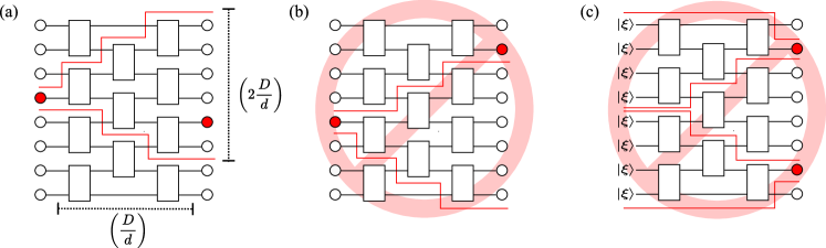
Figure 2: (a) A schematic of the forward lightcone of a 1-$d$ parallel circuit. We employ a paradigmatic scheme such that the left side denotes the input and the right side denotes the output. From the parallel architecture, the size of the lightcone for each dimension is twice of depth for each dimension. (b) An example of a forbidden outcome for FBS, which does not satisfy the constraint (4): input and output photons are not connected by the lightcone. (c) An example of a forbidden outcome for GBS, which does not satisfy the constraint (10): a pair of output photons must be originated from a single source.

To specify the circuit ensemble for random circuit instances, we also define the $d$-dimensional local parallel random circuit, which is $d$-dimensional local parallel circuit with each gate drawn from the Haar measure on U($2$) independently. Such configurations are motivated by recent experimental setups [7, 8, 9, 10]. For the following sections, we consider the $d$-dimensional local parallel (random) circuit as default and prove that the probability distribution is poorly anti-concentrated under a certain polynomial circuit depth, both for FBS and GBS schemes, implying the lack of the average-case hardness for shallow depth circuits.

III.1 Fock-state boson sampling

For FBS, we set the basic parameters as follows. The system is composed of total $M$ modes, and the input state is composed of $N$ single-photon states and vacuum states for the rest modes where $M$ and $N$ are polynomially related by $M=c_{0}N^{\gamma}$ with $\gamma\geq 1$. We use the notation $\bm{t}$ as the position of input single photons, where $\bm{t}\in\mathbb{Z}_{\geq 0}^{N}$ with $1\leq t_{i}\leq M$ and $t_{1}<t_{2}<\cdots<t_{N}$ such that each element $t_{i}$ denotes a mode where a photon is injected. Also, $\bm{s}$ denotes the output photons’ position, where $\bm{s}\in\mathbb{Z}_{\geq 0}^{N}$ with $1\leq s_{i}\leq M$ and $s_{1}\leq s_{2}\leq\cdots\leq s_{N}$ (equality denotes collision outcomes), so each element $s_{i}$ corresponds to a mode where a photon is measured. Here, the number of possible patterns of $\bm{s}$ is given by $\binom{M+N-1}{N}$.

Using those notations, the output probability of FBS to obtain the outcome $\bm{s}$ is expressed as [2]

$$p_{\bm{s}}=\frac{\left|\text{Per}\left(U_{\bm{s},\bm{t}}\right)\right|^{2}}{\bm{s}!}=\frac{1}{\bm{s}!}\left|\sum_{\sigma\in S_{N}}\prod_{j=1}^{N}U_{s_{\sigma(j)},t_{j}}\right|^{2},$$ (2)

where $U_{\bm{s},\bm{t}}$ is a submatrix of circuit unitary matrix $U$ such that $(U_{\bm{s},\bm{t}})_{i,j}=U_{s_{i},t_{j}}$. Also, $\bm{s}!$ denotes a product of the multiplicity of all possible values in $\bm{s}$, and $\sigma\in S_{N}$ denotes permutations along $N$ modes.

As mode interactions cannot occur outside the circuit lightcone, we have $U_{ij}=0$ for $i\notin L_{D}(j)$. Hence, if the size of the lightcone is small such that for given $\bm{s}$, $s_{\sigma(j)}\notin L_{D}(t_{j})$ for all $\sigma\in S_{N}$ and at least one $j\in[N]$, this implies that the given outcome $\bm{s}$ is unphysical, suggesting $p_{\bm{s}}=0$. We can check a simple example of a forbidden outcome of FBS in Fig. 2(b). Intuitively, the number of unphysical outcomes would increase if the lightcone size gets smaller, as photon propagation along different modes becomes more restricted.

From the structure of the local parallel architecture, we find that the size of the lightcone $\left|L_{D}(i)\right|$ grows as

$$\left|L_{D}(i)\right|\leq\left(\frac{2D}{d}\right)^{d},$$ (3)

where $D$ denotes circuit depth and $d$ denotes circuit dimension. The right-hand side of Eq. (3) comes from the fact that the size of the lightcone is $2D/d$ for each dimension as we defined a unit depth as a single step of parallel application of gates (see Fig. 2(a)). Equality holds when the lightcone does not meet geometrical boundaries.

As we can see, for local parallel architecture, lightcones grow polynomially with depth by Eq. (3). Hence, a large portion of outcomes might be unphysical and thus have zero output probability for the low-depth regime (e.g., logarithm depth), as photons are localized inside lightcones of each input mode, whose sizes are very small in this regime. Following the above intuition, we first prove that only an exponentially small portion of the outcomes of FBS is allowed under a certain polynomial depth, regardless of input configurations and ensembles of gates composing the circuit.

Theorem 1.

(Any circuit ensemble) For $d$-dimensional local parallel circuit of depth $D\leq\kappa_{0}N^{\frac{\gamma-1}{d}}$ and arbitrarily chosen input mode configuration, most of the outcomes of FBS have zero output probability for a constant $\kappa_{0}=e^{\frac{1}{d}}c_{0}^{\frac{1}{d}}d/{2}$.

Proof.

From Eq. (2), the probability is non-zero only if at least one path exists between each input and output mode within each lightcone, and this statement can be written as

$$\exists\sigma\in S_{N}\;\forall j\in[N]\;\text{\leavevmode\nobreak\ such that\leavevmode\nobreak\ }\;s_{\sigma(j)}\in L_{D}(t_{j}).$$ (4)

Let $\mathcal{M}$ be the number of outcomes $\bm{s}$ satisfying the constraint (4). Then $\mathcal{M}$ is bounded by

$$\mathcal{M}\leq\prod_{i=1}^{N}\left|L_{D}(t_{i})\right|.$$ (5)

The right-hand side of Eq. (5) counts the outcome by one-to-one correspondence from the input to the output, so at least one output photon is present at each input lightcone, satisfying the constraint (4). Clearly, it is an upper bound for any input configuration $\bm{t}$, because it double-counts the output photon distribution inside the overlapping region of lightcones as photons in the region are indistinguishable. In addition, the inequality at Eq. (5) becomes tighter as the more $L_{D}(t_{i})$ do not overlap each other, which corresponds to input configurations that photon sources are far from each other (e.g., setups from Refs. [18, 20]).

Here we note that $\mathcal{M}$ can be exponentially large in terms of system size, but still, it can be much smaller than all possible output patterns (i.e., $\binom{M+N-1}{N}$). The ratio of permitted outcomes over all possible outcomes, which we will denote as $\Delta$, is bounded by

$$\Delta =\frac{\mathcal{M}}{\binom{M+N-1}{N}}$$ (6)

$$\leq\sqrt{2\pi N}e^{\frac{1}{12N}}\left(\frac{2^{d}D^{d}N}{ed^{d}M}\right)^{N}$$ (7)

$$<3\sqrt{N}\left(\frac{2^{d}D^{d}N^{1-\gamma}}{ed^{d}c_{0}}\right)^{N},$$ (8)

where we used Stirling’s formula and the fact that $N$ is larger than the unity. Here, we only employed the structure of the local parallel architecture (viz., maximal lightcone size), and did not take into account the ensemble the circuit follows. Therefore, the result shows that for depth $D\leq\kappa_{0}N^{\frac{\gamma-1}{d}}$ with a constant $\kappa_{0}=e^{\frac{1}{d}}c_{0}^{\frac{1}{d}}d/{2}$, asymptotically $\Delta$ is exponentially small with system size, regardless of input configuration $\bm{t}$ and circuit ensemble. ∎

Theorem 1 implies that for circuits with a depth below a certain threshold, most output instances have zero probabilities for any circuits. Therefore, most of the output probabilities are easy to approximate for any circuit instance, which undermines the average-case hardness of the output probability approximation for any circuit ensemble.

Furthermore, many current experiments compose their circuits by choosing local beam splitters randomly, i.e., the local parallel random circuit we introduced. In that case, we find that most photons propagate in a region smaller than the actual lightcone, requiring additional circuit depth to get out of the easiness regime.

Theorem 2.

(Local random ensemble) For $d$-dimensional local parallel random circuit of depth $D\leq\alpha_{0}N^{\frac{2(\gamma-1)}{d}-\lambda}$ with a constant $\alpha_{0}=e^{\frac{2}{d}}c_{0}^{\frac{2}{d}}\beta d/{2}$, for any $\lambda>0$, $0<\beta<1$, and input mode configuration, it is easy to estimate the output probabilities of FBS within additive error $\epsilon=\operatorname*{\text{poly}}(N)^{-1}\frac{N!}{M^{N}}$, for $1-\xi$ portion of output instances with probability $1-\delta$ over the random circuit instances, where $\xi$ and $\delta$ are exponentially small with system size.

The term ‘easy’ means that we can approximate the probability well within allowed additive error $\epsilon$ by a trivial algorithm that outputs the value “0”. From the diffusive properties of the local parallel random circuit studied by Ref. [20, 50], we find that the probability distribution is still poorly anti-concentrated below a certain depth which is larger than $\kappa_{0}N^{\frac{\gamma-1}{d}}$.

To sketch the proof of Theorem 2, we define the ‘effective’ lightcone such that truncating the outcomes that at least one photon propagates outside this lightcone results in exponentially small total variation distance from the original distribution, below a certain polynomial depth. In this regime, most of the probability instances are easy to estimate, including the unphysical outcomes and the truncated outcomes (though not unphysical) outside the effective lightcones.

Proof.

See Appendix A. ∎

III.2 Gaussian boson sampling

In this section, we consider an $M$-mode GBS with a product of $K$ single-mode squeezed vacuum (SMSV) states with equal squeezing and vacuum states for the rest modes. We focus on the output photon number $2n$, i.e., there are $n$ pairs of output photons. Now $M$ and $n$ are polynomially related by $M=c_{1}n^{\gamma}$ where $\gamma\geq 1$, and let $K$ be any number satisfying $n\leq K\leq M$. For convenience, we adjust the squeezing parameter such that the mean photon number for our setup is also $2n$, which implies $2n=K\sinh^{2}{r}$. Similarly from the FBS case, we use the notation $\bm{t}$ as the input vector, where $\bm{t}\in\mathbb{Z}_{\geq 0}^{K}$ with $1\leq t_{i}\leq M$ and $t_{1}<t_{2}<\cdots<t_{K}$ such that each element $t_{i}$ denotes a mode where SMSV is injected. Also, $\bm{s}$ denotes an output vector, where $\bm{s}\in\mathbb{Z}_{\geq 0}^{2n}$ with $1\leq s_{i}\leq M$ and $s_{1}\leq s_{2}\leq\cdots\leq s_{2n}$.

Using the above conventions, the probability of obtaining outcome $\bm{s}$ for GBS is proportional to

$$p_{\bm{s}}\propto\left|\text{Haf}\left(\left(U{I}_{K}U^{T}\right)_{\bm{s}}\right)\right|^{2}$$

$$=\left|\sum_{\mu\in\text{PMP}}\prod_{j=1}^{n}\left(\sum_{k=1}^{M}\sum_{l=1}^{M}U_{s_{\mu(2j-1)}k}({I}_{K})_{k,l}U_{s_{\mu(2j)}l}\right)\right|^{2},$$ (9)

where ${I}_{K}$ denotes the projection matrix to the input $K$ modes, and PMP denotes all possible perfect matching permutations along $2n$ modes.

Similar to the FBS case, unphysical outcomes are naturally forbidden as $p_{\bm{s}}=0$. More precisely, If the size of the lightcone is small such that for given $\bm{s}$, $\sum_{k}\sum_{l}U_{s_{\mu(2j-1)}k}({I}_{K})_{k,l}U_{s_{\mu(2j)}l}=0$ for all $\mu\in\text{PMP}$ and at least one $j\in[n]$, then the outcome $\bm{s}$ is forbidden. This phenomenon comes from the fact that the input state is a product of SMSV which is a superposition of even number Fock-states, i.e., photons are always generated as a pair. Therefore, if there exists an output photon such that its backward lightcone does not share the input source with backward lightcones of the other photons, the corresponding outcome is unphysical and thus prohibited. We can check an example of a forbidden outcome of GBS in Fig. 2 (c).

Following the intuition, we prove that only an exponentially small portion of the outcomes of GBS is allowed under a certain polynomial depth, regardless of input configurations and ensembles of gates composing the circuit.

Theorem 3.

(Any circuit ensemble) For $d$-dimensional local parallel circuit of depth $D\leq\kappa_{1}n^{\frac{\gamma-1}{d}}$, arbitrary $K$ within $n\leq K\leq M$ and arbitrarily chosen input mode configuration, most of the outcomes of GBS have zero output probability for a constant $\kappa_{1}=c_{1}^{\frac{1}{d}}e^{\frac{1}{d}}d/2^{\frac{1}{d}+2}$.

Proof.

The probability of GBS is non-zero only if $2n$ output photons are paired up and share the input source inside their backward lightcones, and this statement can be written as

$$\exists\mu\;\forall j\;\exists i\;\text{\leavevmode\nobreak\ such that\leavevmode\nobreak\ }\;t_{i}\in L_{D}^{{\dagger}}(s_{\mu(2j-1)})\cap L_{D}^{{\dagger}}(s_{\mu(2j)}).$$ (10)

Since we want to upper-bound the number of permitted outcomes, we alleviate the constraint (10) by taking $K=M$, which denotes the full-mode input. Then, from (10), the constraint for the index $i$ vanishes and the last term reduces to $L_{D}^{{\dagger}}(s_{\mu(2j-1)})\cap L_{D}^{{\dagger}}(s_{\mu(2j)})\neq\emptyset$ . Then we can approximately count the number of possible outcomes as follows: $(i)$ Pick $n$ pairs over $M$ modes with replacement. $(ii)$ Count all possible alignment for each $n$ pair connected by lightcones.

Let $\mathcal{M}$ be the number of outcomes $\bm{s}$ satisfying the constraint (10). Then $\mathcal{M}$ is bounded by

$$\mathcal{M}\leq\frac{1}{2^{n}}\sum_{\textbf{r}}\prod_{i=1}^{n}\left|L_{D}\circ L_{D}^{{\dagger}}(r_{i})\right|,$$ (11)

where $\bm{r}\in\mathbb{Z}_{\geq 0}^{n}$ with $1\leq r_{i}\leq M$ and $r_{1}\leq r_{2}\leq\cdots\leq r_{n}$ denotes the possible mode selection at step $(i)$ so the number of possible alignment of $\bm{r}$ is $\binom{M+n-1}{n}$. The factor $\frac{1}{2^{n}}$ comes from the indistinguishability of the photons between step $(i)$ and $(ii)$. As we allowed double counting at overlapping regions and weakened the constraint (10) by taking $K=M$, the right-hand side of Eq. (11) certainly implies an upper bound.

From the structure of $d$-dimensional parallel circuit architecture, with generalization of Eq. (3), $|L_{D}\circ L_{D}^{{\dagger}}(r_{i})|$ has the corresponding bound

$$\left|L_{D}\circ L_{D}^{{\dagger}}(r_{i})\right|\leq\left(\frac{4D}{d}\right)^{d},$$ (12)

where equality holds when lightcones do not meet geometrical boundaries. Now $\Delta$ is the ratio of outcomes satisfying (10) over all possible output distributions, and it is bounded by

$$\Delta =\frac{\mathcal{M}}{\binom{M+2n-1}{2n}}$$ (13)

$$\leq\frac{1}{2^{n}}\left[4^{d}\left(\frac{D}{d}\right)^{d}\right]^{n}\frac{\binom{M+n-1}{n}}{\binom{M+2n-1}{2n}}$$ (14)

$$\leq\sqrt{2}e^{\frac{1}{24n}}\left(\frac{2^{2d+1}D^{d}}{ed^{d}}\frac{n}{M}\right)^{n}$$ (15)

$$<2\left(\frac{2^{2d+1}}{ed^{d}c_{1}}D^{d}n^{1-\gamma}\right)^{n}.$$ (16)

We used Stirling’s formula and the fact that $n$ is larger than the unity. This result shows that for depth $D\leq\kappa_{1}n^{\frac{\gamma-1}{d}}$ with $\kappa_{1}=c_{1}^{\frac{1}{d}}e^{\frac{1}{d}}d/2^{\frac{1}{d}+2}$, $\Delta$ is exponentially small with system size, regardless of $K$ in $n\leq K\leq M$ and distribution of $\bm{t}$. Also, as we only used the structure of the local parallel architecture, the result holds for any circuit ensemble. ∎

Theorem 3 states that regardless of the number of input SMSV states and their configuration, most of the outcomes of GBS have zero probabilities which are easy to approximate under a certain degree of polynomial depth, for any circuit instances. Moreover, for the case of the local parallel random circuit, we prove that the argument from the proof of Theorem 2 holds even for the GBS scheme, requiring additional depth to get out of a poorly anti-concentrated regime.

Theorem 4.

(Local random ensemble) For $d$-dimensional local parallel random circuit of depth $D\leq\alpha_{1}n^{\frac{2(\gamma-1)}{d}-\lambda}$ with $\alpha_{1}=c_{1}^{\frac{2}{d}}e^{\frac{2}{d}}\beta d/{2}^{\frac{2}{d}+3}$, for any $\lambda>0$,$0<\beta<1$, $n\leq K\leq M$ and input mode configuration, it is easy to estimate the output probabilities of GBS within additive error $\epsilon=\operatorname*{\text{poly}}(n)^{-1}\frac{(2n)!}{M^{2n}}$ for $1-\xi$ portion of output instances with probability $1-\delta$ over the random circuit instances, where $\xi$ and $\delta$ are exponentially small with system size.

Proof.

See Appendix B. ∎

IV Geometrically non-local architecture: hypercubic structure

So far, we have shown that the $d$-dimensional local parallel circuit is faced with the limit for achieving sampling hardness at shallow depth. As the size of the lightcone of the local architecture grows polynomially with depth, a mode connectivity issue arises below a certain polynomial depth, which leads to the prohibition of most of the outcomes and thus undermines the average-case hardness. Also, as the random instances of the circuit are characterized by diffusive dynamics, most of the photon propagation is determined by the effective lightcone whose size is smaller than the original one, which requires additional depth to resolve the mode connectivity issue. The problem is that from the photon loss model for each unit depth, polynomial depth entails large noise that disturbs classical intractability.

Since the problems we addressed come from circuit architecture which allows only local interactions, an obvious way to resolve those problems is to consider non-local interactions along modes, i.e., for the case that geometrically non-local unitary gates are available. Allowing the non-local interactions, we find a circuit that can mitigate the issues about connectivity and diffusive property within logarithmic circuit depth, where the architecture of the circuit has been used in numerical linear algebra in order to construct structured matrices efficiently [53, 54, 55]. Throughout this section, we refer to the circuit as a non-local hypercubic structure (NLHS) circuit for simplicity, and an example of the circuit architecture for mode number $M=16$ is illustrated in Fig. 3.

Figure 3: A Schematic of a one-cycle of NLHS circuit for total mode number $M=2^{4}$. In this case, the architecture of the circuit can be interpreted as a 4$d$ hypercube, also known as a tesseract. Here, each color implies a depth unit, as all of the unitary gates with the same color are applied in parallel.

IV.1 Structure of the circuit

Let the total mode number be $M=2^{p}$ (for some integer $p$) for convenience. The sequence for the construction of a one-cycle of NLHS circuit is simple: for each $D=1,2,\cdots,p$, apply unitary gates between mode number $2^{D}(j-1)+k$ and $2^{D}(j-1)+k+2^{D-1}$, for all $j=1,2,\cdots,2^{p-D}$ and $k=1,2,\cdots,2^{D-1}$. Here, we point out that each $D$ implies the unit depth in terms of our standard, as unitary gates are applied in parallel for all $j$ and $k$ indices (e.g., all of the unitary gates with the same color in Fig. 3 are applied in unit depth). The corresponding circuit architecture has a well-spreading property such that photons departed from any mode can spread $2^{D}$ modes for depth $D$, and thus fully connected for the one-cycle of the circuit, viz., at least one path exists from any input mode toward any output mode. Additionally, even for arbitrary $M$, we can still achieve full mode connection in $\mathcal{O}(\log M)$ depth by iterating the above process (e.g., by stacking one-cycle of the circuit with depth $\lfloor\log M\rfloor$ on the left side and right side of the modes, alternatively). Even so, to simplify the analysis, we only consider the case of $M=2^{p}$ with a fixed $p\in\mathbb{N}$ for the rest of the section and define a single round of NLHS circuit as the one-cycle of the sequence we introduced, i.e., the procedure up to circuit depth $D=p$.

The NLHS circuit architecture indeed satisfies the minimum requirement for achieving average-case hardness in a low-depth regime, namely, having accessibility to all outcomes in a single round of the circuit. Now we consider the case that the circuit is randomly drawn from a specific circuit ensemble, to examine whether the probability distribution can satisfy the condition of average-case hardness. Specifically, we use a typical setup such that all unitary gates composing the NLHS circuit as independently chosen random beam splitters, each drawn from Haar measure on U(2), similar to the local parallel random circuit case. From now on, we define the corresponding circuit as random NLHS circuit.

We first find that a single round of the random NLHS circuit has evenly spreading property in terms of single-photon propagation, compared to the localized property (i.e., diffusive dynamics) of the local parallel random circuit. We can check this property with an absolute squared unitary element averaging over random circuit instances, which corresponds to the average of single-photon transition amplitude between modes. Let $U_{i,j}^{D}$ be a unitary element for the circuit with depth $D$. Using properties of random beam splitters each drawn from Haar measure on U(2), an average of an absolute squared unitary element becomes

$$\operatorname*{\mathbb{E}}[|U_{i,j}^{p}|^{2}] =\frac{1}{2}\operatorname*{\mathbb{E}}[|U_{i,j}^{p-1}|^{2}]+\frac{1}{2}\operatorname*{\mathbb{E}}[|U_{i,j\pm 2^{p-1}}^{p-1}|^{2}]$$ (17)

$$=\frac{1}{4}\operatorname*{\mathbb{E}}[|U_{i,j}^{p-2}|^{2}]+\frac{1}{4}\operatorname*{\mathbb{E}}[|U_{i,j\pm 2^{p-2}}^{p-2}|^{2}]$$

$$+\frac{1}{4}\operatorname*{\mathbb{E}}[|U_{i,j\pm 2^{p-1}}^{p-2}|^{2}]+\frac{1}{4}\operatorname*{\mathbb{E}}[|U_{i,j\pm 2^{p-1}\pm 2^{p-2}}^{p-2}|^{2}]$$ (18)

$$=\cdots$$

$$=\frac{1}{2^{p}}\sum_{j=1}^{M}\operatorname*{\mathbb{E}}[|U_{i,j}^{0}|^{2}]$$ (19)

$$=\frac{1}{2^{p}}$$ (20)

by averaging over the beam splitters for each depth, where $\pm$ signs behind index $j$ are determined by the binary notation of $j$. Interestingly, the result shows that a single round of random NLHS circuit can mimic the Haar unitary up to the first moment.

Also, if we repeat a single round of random NLHS circuit $\mathcal{C}$ times (i.e., total $\mathcal{C}\log M$ depth, iteratively stacking a single round of NLHS circuit of depth $D=\log M$), the number of paths between arbitrary modes scales as $M^{\mathcal{C}-1}$. To be more detailed, as a path between arbitrary modes is uniquely determined for a single round of NLHS circuit, the number of paths between arbitrary modes grows as $1,M,M^{2},\cdots$ by repeating the circuit. This exponential growth of possible paths motivates us to elucidate the properties of the random NLHS circuit and how the repetition of the corresponding circuit works on those properties.

For the following two sections, we propose numerical evidence that the random NLHS circuit quickly converges to the global Haar random unitary (i.e., random unitary drawn from Haar measure on U($M$)) by repeating a single round of the random circuit drawn independently for each repetition. Specifically, we examine the probability distribution and entanglement generation of the random NLHS circuit with different repetition numbers and their convergence behavior toward the global Haar random unitary circuit.

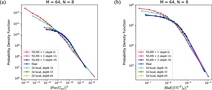
Figure 4: Probability density function for output probabilities of (a) FBS and (b) GBS with $M=64$ and $N=8$, for random NLHS circuit with different repetition numbers and 2$d$ local parallel random circuit with different depths. The distribution corresponding to the global Haar unitary circuit is also displayed as an ideal case. The $x$-axis is for the (unnormalized) output probability values, and the y-axis is for the corresponding densities along the samples. Input $\bm{t}$ and output $\bm{s}$ are chosen randomly along possible configurations of $N$ photons along $M$ modes, without collision.

IV.2 Probability distribution of random NLHS circuit

We investigate the output probability distribution of FBS and GBS over the random NLHS circuit (with repetitions) instances and its resemblance to the distribution from the global Haar random unitary. To statistically analyze the output probabilities over the randomly chosen circuit instances, we employ the probability density function, which is a modified version of the histogram and employed by Ref. [2] to numerically show evidence of the anti-concentration property of FBS (for more details, see Fig. 5 in Ref. [2]). The reason we use the probability density function is for enhanced visibility, as we observed that the degree of concentration of output probability distribution dramatically changes with circuit depth.

The difference from the histogram is, instead of using equal intervals on the density axis, each interval now contains equal numbers of samples. Specifically, samples sorted in ascending order are divided into each bucket, containing an equal number of samples. Next, the density of each bucket is determined by the fraction of samples it contains divided by its width, where the width of the bucket is the difference between the maximum and minimum value of samples in the bucket. The probability density function is a plot of those densities corresponding to each bucket, where the $x$-axis represents the value of each sample. Throughout this section, we fix the number of output probability instances for each unitary circuit as 10000 and fix the number of buckets as 20, so a single point of the density function contains 500 output probability instances.

For output probabilities, we use $|\text{Per}(U_{\bm{s},\bm{t}})|^{2}$ for the FBS scheme, which corresponds to the output probability of FBS to get output $\bm{s}$ from input $\bm{t}$. Also, we use $|\text{Haf}((UU^{T})_{\bm{s}})|^{2}$ for the GBS scheme, which corresponds to the unnormalized output probability of GBS to get output $\bm{s}$ from full-mode SMSV input state with equal squeezing. To simplify the analysis, we fix the output photon number of GBS.

IV.2.1 Comparison with the local parallel circuit

Using the probability density function, we first compare the performance of the random NLHS circuit and typical 2$d$ local parallel random circuit, for fixed mode number $M=64$ and photon number $N=8$. In this case, a single round of random NLHS circuit can be implemented with circuit depth $D=\log M=6$, and thus $\mathcal{C}$ repetition of the circuit requires $6\mathcal{C}$ depth. Here, we consider the repetition number $\mathcal{C}$ up to three (i.e., up to $D=18$), with the random circuit drawn independently for each repetition. Also, for the 2$d$ local parallel random circuit, we consider circuit depth from $D=16$, not to restrict photon propagation between arbitrary modes.

We randomly sample 10000 unitary matrices for each circuit with different depths and calculate the output probability of randomly chosen collision-free input/output (only random collision-free output for GBS) for each unitary matrix we sampled. Here, we can focus on collision-free cases if $M$ is much larger than $N$ such that $N=\mathcal{O}(\sqrt{M})$ [2], which fits well with our setup. Using those probability values, we plot the probability density function in Fig. 4, for random NLHS circuits with different repetition numbers, and for 2$d$ local random circuits with different depths. We also plot the function corresponding to $M$ dimensional Haar random unitary circuit, as an ideal case. The dispersion of the distribution along the $x$-axis implies a variance of output probability values over the random instances, such that the less dispersed the distribution implies the more the corresponding output probability distribution is anti-concentrated.

We find that distributions from both circuits converge to a distribution from $M$ dimensional Haar random unitary as increasing depth, which is predictable from the convergence properties studied at [56, 57]. However, their convergence behavior toward global Haar random unitary is different. Specifically, although a single round of random NLHS circuit has poor performance in terms of anti-concentration, an iteration of the random NLHS circuit makes quick convergence to the distribution of the Haar random unitary, both for FBS and GBS schemes.

IV.2.2 Convergence to the behavior of the global Haar measure, for different system sizes

To identify how the convergence behavior varies as system size scales, we further investigate the number of repetitions of the random NLHS circuit required for the convergence to the global Haar random unitary with increasing system size. Here, we also examine the repetition number up to three with the random circuit drawn independently for each repetition. We set mode numbers $M=32,64,128,256$ and randomly sample 10000 unitary matrices for each repetition of the random NLHS circuit and for $M$ dimensional Haar random unitary circuit. Then we calculate the output probability of randomly chosen input/output for each matrix, both for FBS and GBS schemes, given output photon number $N$ around $\sqrt{M}$. We plot the probability density function for those values in Fig. 5.

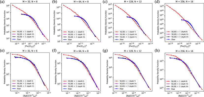
Figure 5: Probability density function for (a-d) FBS and (e-h) GBS, with $M=32,64,128,256$ and $N=6,8,12,16$ each. For each figure, the distributions corresponding to the random NLHS circuit, with repetition numbers up to three, are presented. Also, the distribution of the Haar unitary is displayed as an ideal case. Input $\bm{t}$ and output $\bm{s}$ are chosen randomly along possible configurations of $N$ photons along $M$ modes, without collision.

Interestingly, the number of repetitions required to imitate the distribution from the global Haar random unitary is insensitive to system size. More specifically, stacking the random NLHS circuit twice dramatically changes its distribution, showing a close resemblance to the distribution from the global Haar unitary, which implies the existence of critical behavior between stacking the circuit once and twice. Here, the mode numbers we used (up to 256 modes) cover all recent experimental results of GBS [7, 8, 9], even though the photon numbers we used are small compared to those results. Therefore, up to the system size covered by near-term experiments, the random NLHS circuit can imitate output probability distributions of fixed photon number $N\sim\sqrt{M}$ from the global Haar random unitary circuit with considerably low depth. Also, as the required repetition number for imitation is insensitive to the system size, the result gives hope that the low-depth circuit (a few repetitions of the random NLHS circuit) can well approximate the Haar unitary and thus suggests evidence of the average-case hardness for larger quantum systems.

We also examine the scaling behavior of Haar measure convergence in terms of photon number $N$, for fixed mode number $M$. We plot the probability density function for fixed mode number $M=32$ with output photon numbers $N=8,16$ both for FBS and GBS schemes, which can be checked in Appendix C. The result shows similar behavior, i.e., the number of repetitions required does not change a lot as the output photon number increases. Hence, the result suggests a possibility such that a low-depth random NLHS circuit can even imitate output probability distributions from the global Haar random unitary for output photon number much larger than $\mathcal{O}(\sqrt{M})$, which is also remarkable.

IV.2.3 Hiding property

Additionally, we investigate if hiding property holds for the random NLHS circuit. The hiding theorem of BS shows two properties [2, 4]. One is that probability distribution is output independent, i.e., the probability of any outcome instances follows the same distribution over random circuit instances. The other is that the corresponding output probability is similar to the quantity which is conjectured to be hard to estimate on average, viz., squared permanent (hafnian) of random Gaussian matrices. We numerically investigate both of the above properties using the probability density function; readers who are interested in this subject can see the result in Appendix D.

IV.3 Entanglement generation of random NLHS circuit

In this section, we investigate how entanglement along the modes varies with the repetition of the NLHS circuit, to show the simulation hardness and the convergence behavior toward the global Haar measure from a different perspective. Entanglement is considered necessary for the hardness of classical simulation of a quantum state, as various tensor network methods can approximate the low entangled state efficiently [14, 15, 16]. Rényi entropies are often cited as a measure of entanglement, and possibly indicate the feasibility of simulating the given quantum state via those methods [58, 59]. Specifically, restricting to bosonic Gaussian states, many results [60, 61, 62] suggested that Rényi-2 entropy is a good measure of entanglement. Moreover, Ref. [63] recently proposed the Rényi-2 Page curve of pure Gaussian state evolved by the global Haar random unitary, exactly the output state of the ideal GBS scheme. Hence, to examine the entanglement behavior, we focus on the Rényi-2 entropy of reduced states of the output states of GBS, each evolved by different repetitions of random NLHS circuits or global Haar random unitary. Our goal is to examine the entanglement generation of the random NLHS circuit with increasing depth and investigate if the circuit with increasing depth can reproduce the Rényi-2 Page curve, to propose evidence of the simulation hardness of GBS for the corresponding circuit and its convergence behavior toward the global Haar random unitary.

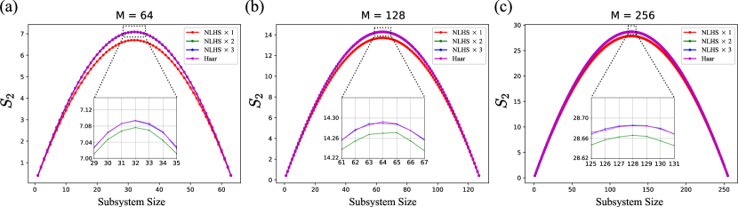
Figure 6: The average of Rényi-2 entropy with respect to different subsystem sizes, for mode number (a) $M=64$, (b) $M=128$, (c) $M=256$. For each figure, the average of entropy values corresponding to the Gaussian state evolved by various repetitions of random NLHS circuits and $M$ mode Haar random unitary circuits, are presented.

For mode numbers $M=64,128,256$, we randomly sample 10000 unitary matrices from each repetition of the random NLHS circuit, and also from the global Haar measure as an ideal case. Then the $M$ product of SMSV with equal squeezing parameter $r=0.4$ is evolved with those unitary matrices. To calculate the entropy of the output states, $M$ modes are partitioned into two groups, one for $k$ modes and the other for $M-k$ modes, where the mode selection is completely random along ${}_{M}C_{k}$ possible combinations. For all $k\in[M-1]$, we calculate the entropy of a reduced state and average over the unitary matrices, while the Rényi-2 entropy takes the form of $S_{2}=\frac{1}{2}\log\det\sigma$, where $\sigma$ is the covariance matrix of the reduced state [64].

In Fig. 6, we plot the average of Rényi-2 entropy with respect to different subsystem sizes, for each mode number we fixed. The result shows the entanglement generation of the random NLHS circuit with an increasing stacking number, where the distribution converges to the Rényi-2 Page curve (i.e., distribution from the global Haar random unitary) as circuit depth increases. It is notable that the required number of repetitions for the convergence is insensitive to system size, similar to previous results we addressed. Specifically, stacking the random NLHS circuit twice or more resembles the behavior of the global Haar measure, and the absolute difference of the entropy values between them varies very slowly with system size, which is also remarkable.

IV.4 Experimental realization of NLHS circuit

Throughout the previous two sections, we have numerically shown that the random NLHS circuit shows quick convergence behavior toward Haar unitary distribution by a few repetitions, which gives a possibility for the average-case hardness of BS with shallow-depth quantum circuits. In this section, we discuss the experimental feasibility of the random NLHS circuit. Experimental realization of the random NLHS circuit (with repetitions) requires a geometrically non-local setup or a high-dimensional architecture with its dimension up to $d=\log M$.

Considering photonic systems, Ref. [65] implemented integrated photonic chips for $2^{d}$ modes with dimensions up to $d=3$, where the interaction along modes occurs in hypercubic sequence, precisely the circuit architecture of the NLHS circuit. Hence, implementation of the random NLHS circuit would be feasible if the dimension of those devices can be increased in a scalable manner and if the gates composing the devices are programmable. Additionally, we can employ high-dimensional photonic architecture used in [4, 9] but in a different gate sequence, i.e., the hypercubic sequence we used. Optical frequency crystals, as demonstrated in [66, 67], would be a viable alternative, which can also suggest high-dimensional photonic architecture as the NLHS circuit.

We can also consider phononic systems, such as trapped ions, which can be utilized as alternative bosons to construct linear-optical circuits [68, 69, 70]. Specifically, recent works from [71] have experimentally demonstrated a programmable all-to-all setup for four modes of phononic network with trapped ions, using collective-vibrational modes of ions. Although architectures based on trapped ions might face the limitation of long-range interaction due to spectral crowding when system size scales, employing modular architecture would help overcome this problem. Therefore, this setup may also offer a promising candidate for the experimental realization of the random NLHS circuit in the near future.

V Discussion

In this work, we examined that for local circuit architecture, the depth of the linear optical circuit should be large enough to satisfy the conditions for the sampling hardness based on the currently available proof technique. More precisely, for depth under the degree of $\mathcal{O}(M^{\frac{(\gamma-1)}{\gamma d}})$, most of the probabilities are zero regardless of circuit ensemble and input configuration. Besides, for local random ensemble, most of the probabilities are too small and easy to estimate for depth under $\mathcal{O}(M^{\frac{1}{\gamma}[\frac{2(\gamma-1)}{d}-\lambda]})$. We interpreted that this problem comes from the properties of the local parallel architecture, where the circuit lightcone grows polynomially with depth, and the circuit is characterized by the diffusive property, which hinders anti-concentration. We proposed the circuit architecture using non-local interactions, which can restrain the issues we addressed at logarithm circuit depth. Also, the repetition of the random NLHS circuit shows quick convergence behavior toward the global Haar random unitary, where the speed of convergence is insensitive to the system size. Hence, we conclude that the corresponding circuit can be used for approximate Haar measure with shallow depth circuit, and has the potential to be utilized as an architecture for scalable quantum advantage with BS.

Here are a few remarks about our results and related open questions:

1. It is worth emphasizing the difference of our result from the one in Ref. [4] which provides evidence of the hardness of sampling from the high dimensional circuit of constant depth. We stress that our depth unit is different from the depth definition in Refs. [4, 9], where the difference comes from the structural difference of the circuit architecture. Specifically, they denote unit depth by one cycle of serial application of gates along the modes for each dimension, which translates to depth $\mathcal{O}(M)$ from our standard such that only parallel implementation of gates is allowed for unit depth.

2. The key difference between RCS and BS with shallow-depth quantum circuits lies in the accessibility of outcomes, which comes from a systematic difference. In RCS, as each outcome is obtained through measurement on a computational basis, the local Pauli-X operator on each qubit gives access to all possible outcomes. Hence, when a circuit for RCS is constructed using local Haar unitaries, all of the outcomes are accessible regardless of the circuit depth, and output symmetry from random circuit instances is easily established by the translation invariance of the Haar measure over the local random unitary gates. However, in the case of BS, each outcome is obtained through measurement on a photon number basis; the accessibility of outcomes can be restricted in low-depth regimes as we have shown. Since the current proof of the sampling hardness requires the usage of all possible outcomes (as the allowed error is given by total variation distance), we emphasize that the circuit architecture for BS must be carefully designed. In this regard, the NLHS circuit we proposed may play an important role in the shallow-depth hardness argument as it gives access to all possible outcomes at logarithm depth.

3. As we discussed in Sec. II, the measure over $M$ mode random NLHS circuits with a few repetitions cannot strictly imitate the Haar measure on U($M$) unless the repetition number satisfies $\Omega(M)$. However, even though there is only numerical evidence yet, the repetition of the random NLHS circuit can well approximate certain properties (output probability distribution, entanglement generation) of the global Haar random unitary. This implies that approximating Haar measure might be possible only with a few repetitions of the circuit [56, 57]. Our results raise an open question of how much the measure over the random circuit matrices can imitate the global Haar measure, with increasing repetition numbers.

4. A few repetitions of the random NLHS circuit show global randomness for fixed-size numerical experiments, which gives a possibility to show the average-case hardness of output probability approximation at a shallow depth regime, for the asymptotic limit. As we discussed in the introduction, there is a possibility that a constant number of repetitions of the random NLHS circuit (i.e., logarithm depth circuit) may enable us to avoid the classically simulable regime of noisy BS with photon loss. Specifically, as the output photon number is given by $N_{\text{out}}=NT^{D}$ for circuit depth $D$, asymptotically $N_{\text{out}}$ can be larger than $\mathcal{O}(\sqrt{N})$ for $D=\mathcal{O}(\log N)$. Therefore, another open problem would be to show the average-case hardness of approximating output probabilities from a few repetitions of the random NLHS circuit, for the case that noises are applied at each depth.

Appendix A Proof of Theorem 2

In this Appendix, we provide the proof of Theorem 2.

Proof.

We first follow the process of approximating the output probability distribution of the local parallel random circuit using unitary matrix truncation; more details can be found in Refs. [50, 20]. It is known that photons follow classical random walk behavior on average in the local parallel random circuit. From this behavior, they are effectively localized in a regime even smaller than a given lightcone; we can find a bound of the regime such that the probability of leakage from this regime is exponentially small. In this case, truncation of the circuit unitary matrix by discarding matrix elements outside the regime results in an exponentially small total variation distance from the original output distribution. This implies that the summation of output probabilities that at least one photon propagates outside the regime would also be exponentially small.

To be more specific, we define a leakage rate from the input mode $i$ as $\eta_{i}(l)\coloneqq\sum_{j}^{{}^{\prime}}|U_{j,i}|^{2}$, where the summation is over the all possible modes that are geometrically away from the mode $i$ more than length $l$ for each dimension. From the classical random walk behavior, when the length $l$ satisfies the corresponding bound

$$l\geq\sqrt{\frac{2N^{\lambda}D}{\beta d}},$$ (21)

with any constant $\lambda>0$ and $0<\beta<1$, then $\Pr\left[\eta_{i}(l)\leq\exp(-N^{\lambda})\right]\geq 1-\delta$ where $\delta\leq 2d\exp\left[(1-\frac{1}{\beta})N^{\lambda}\right]$, and the probability is over the random instances of the circuit.

We define a matrix $\tilde{U}$, a truncated version of a unitary matrix $U$, by discarding the matrix elements that are farther than $l$ for each dimension from the given column index. From this definition, $\tilde{U}\equiv U-dU$ with $\|dU\|_{F}^{2}=\sum_{i}\eta_{i}(l)$, where the summation is over all possible column indices. If $l$ satisfies Eq. (21), then $\|dU\|_{F}^{2}\leq\text{poly}(N)\exp(-N^{\lambda})$ with probabilty $1-\delta$ over the circuit instances. Using this fact with results from [72], we can deduce that the total variation distance between distributions from $U$ and $\tilde{U}$ is bounded by $\operatorname*{\text{poly}}(N)\|dU\|_{F}^{2}$ which is exponentially small with system size for our case. Hence, the summation of probabilities of outcomes corresponding to the discarded elements, i.e. the outcomes that at least a single photon propagates from the source more than $l$ satisfying Eq. (21), is bounded by the total variation distance which is exponentially small with high probability.

However, as $\tilde{U}$ is not a unitary matrix, the output distribution of the matrix cannot be determined. We can resolve this issue by first extending $\tilde{U}$ to a unitary matrix in $2M\times 2M$, which contains normalized $\tilde{U}$ at first $M$ modes, and post-selecting the outcomes only at the first $M$ modes. This way, we can get the probability distribution corresponding to $\tilde{U}$ (see [20] for more details). To summarize, the summation of probabilities of the outcomes outside the regime $l$ has the order of maximally $\text{poly}(N)\exp(-N^{\lambda})$ with probability $1-\delta$ over the circuit instances.

We define an effective lightcone $L_{D}^{{}^{\prime}}$ such that the size of the lightcone for each dimension has a minimum value satisfying Eq. (21). Following the above discussions, the summation of probabilities of the outcomes outside the effective lightcone is exponentially small with high probability. Hence, if the portion of outcomes inside the effective lightcone is exponentially small, the output probability distribution is concentrated on the small portion of the outcomes.

Let $\mathcal{M}^{\prime}$ number of outcomes $\bm{s}$ satisfying the constraint (4), but now the lightcone term is replaced by the effective lightcone $L_{D}^{{}^{\prime}}(t_{i})$. Upper bound of $|L_{D}^{{}^{\prime}}(t_{i})|$ is

$$\left|L_{D}^{{}^{\prime}}(t_{i})\right|\leq\left(\frac{2N^{\lambda}D}{\beta d}\right)^{\frac{d}{2}},$$ (22)

where equality holds when the effective lightcone does not meet geometrical boundaries. The ratio of outcomes inside the effective lightcone over all possible outcomes $\Delta^{\prime}$ is

$$\Delta^{\prime} =\frac{\mathcal{M}^{\prime}}{\binom{M+N-1}{N}}$$ (23)

$$\leq\sqrt{2\pi N}e^{\frac{1}{12N}}\left[\frac{N}{eM}\left(\frac{2N^{\lambda}D}{\beta d}\right)^{\frac{d}{2}}\right]^{N}$$ (24)

$$<3\sqrt{N}\left[\frac{1}{ec_{0}}\left(\frac{2}{\beta d}\right)^{\frac{d}{2}}D^{\frac{d}{2}}N^{1-\gamma+\frac{\lambda d}{2}}\right]^{N}.$$ (25)

Indeed, for the depth $D\leq\alpha_{0}N^{\frac{2(\gamma-1)}{d}-\lambda}$ with a constant $\alpha_{0}=e^{\frac{2}{d}}c_{0}^{\frac{2}{d}}\beta d/{2}$, most of the probability distribution is concentrated inside the exponentially small portions of outcomes.

Our proof of Theorem 2 is not completed yet because the statement that the summation of truncated probabilities is smaller than $\text{poly}(N)\exp(-N^{\lambda})$ does not guarantee that all single truncated probabilities are small enough to estimate easily. There may exist some truncated probabilities larger than the allowed additive error $\epsilon$, which we cannot safely estimate as zero.

Nevertheless, we can verify that the truncated outcomes outside the effective lightcones having probabilities larger than given $\epsilon$ cannot occupy large portions of outcomes. Let $\Gamma$ be the ratio of truncated outcomes having probabilities larger than $\epsilon$ over all possible outcomes of FBS. Also, let $\mathcal{S}^{\prime}$ set of outcomes outside the effective lightcone, so $|\mathcal{S}^{\prime}|=(1-\Delta^{\prime})\binom{M+N-1}{N}$.

We find the upper bound of $\Gamma$ as

$$\Gamma \leq\Pr_{\bm{s}\in\mathcal{S}^{\prime}}\left[p_{\bm{s}}\geq\epsilon\right]$$ (26)

$$\leq\frac{1}{\epsilon}\operatorname*{\mathbb{E}}_{\bm{s}\in\mathcal{S}^{\prime}}\left[p_{\bm{s}}\right]$$ (27)

$$=\frac{1}{\epsilon}\frac{\sum_{\bm{s}\in\mathcal{S}^{\prime}}p_{\bm{s}}}{(1-\Delta^{\prime})\binom{M+N-1}{N}}$$ (28)

$$\leq\frac{1}{\epsilon}\frac{N!}{M^{N}}\operatorname*{\text{poly}}(N)\exp(-N^{\lambda}),$$ (29)

where we used Markov’s inequality for Eq. (27) and the inequality Eq. (29) holds with probability $1-\delta$ over the circuit instance. Therefore, for $\epsilon=\operatorname*{\text{poly}}(N)^{-1}\frac{N!}{M^{N}}$, $\Gamma\leq\operatorname*{\text{poly}}(N)\exp(-N^{\lambda})$ with probability $1-\delta$ over the circuit instances.

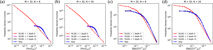
Figure 7: Probability density function for (a-b) FBS and (c-d) GBS, with $M=32$ and $N=8,16$ each, Input $\bm{t}$ and output $\bm{s}$ are fixed at first $N$ modes over $M$ modes. The distributions corresponding to the random NLHS circuit, with repetition numbers up to three, are presented. Also, the distribution of the Haar unitary is displayed as an ideal case.

In summary, for depth $D\leq\alpha_{0}N^{\frac{2(\gamma-1)}{d}-\lambda}$ with a constant $\alpha_{0}=e^{\frac{2}{d}}c_{0}^{\frac{2}{d}}\beta d/{2}$, the ratio of outcomes we cannot easily estimate their probabilities within additive error $\epsilon$, which can be characterized by $\xi\equiv\Delta^{\prime}+\Gamma$, is exponentially small with probability larger than $1-\delta$ over the circuit instances. This completes the proof. ∎

Appendix B Proof of Theorem 4

In this Appendix, we provide the proof of Theorem 4.

Proof.

We use the concept of effective lightcone as well for GBS, except for the notation change from $N$ to $n$. Similar to the FBS case, using truncation of unitary matrix by the effective lightcone, summation of probabilities of the outcomes outside the effective lightcone has the order of maximally $\text{poly}(n)\exp(-n^{\lambda})$ with probability $1-\delta$ over the circuit instances. Here, $\delta\leq 2d\exp\left[(1-\frac{1}{\beta})n^{\lambda}\right]$ with any $\lambda>0$ and $0<\beta<1$.

Here, the truncated outcomes can have any output photon numbers, contrary to our scheme that focuses on fixed output photon number $2n$. Hence, the summation of truncated probabilities can be enlarged from $\text{poly}(n)\exp(-n^{\lambda})$ if we normalize the output probability distribution in the $2n$ photon subspace. However, it is not problematic if we also set the mean photon number $2n$, as the output probability of getting the mean photon number is at least an inverse polynomial of system size. Specifically, the probability of generating $2n$ output photon events is given by negative binomial distribution [3]

$$P(2n)=\binom{K/2+n-1}{n}\frac{\tanh^{2n}r}{\cosh^{K}r}.$$ (30)

By applying $2n=K\sinh^{2}{r}$, the above probability reduces to $P(2n)=\Omega(n^{-\frac{1}{2}})$, which is indeed an inverse polynomial. Hence, even considering only the $2n$ photon outcomes, the summation of probabilities truncated by effective lightcone still have the order of maximally $\text{poly}(n)\exp(-n^{\lambda})$.

From the above discussions, if the ratio of outcomes inside the effective lightcone is exponentially small, this means that the output probability distribution is concentrated on the exponentially small portion of the outcomes. Let $\mathcal{M}^{\prime}$ number of outcomes satisfying (10), but now the lightcone is replaced by the effective lightcone $L_{D}^{{}^{\prime}}$. We can similarly use Eq. (11) but now Eq. (12) is modified to

$$\left|L_{D}^{{}^{\prime}}\circ{L_{D}^{{}^{\prime}}}^{{\dagger}}(r_{i})\right|\leq 2^{d}\left(\frac{2n^{\lambda}D}{\beta d}\right)^{\frac{d}{2}}.$$ (31)

The ratio of outcomes inside the effective lightcone over all possible outcomes $\Delta^{\prime}$ is

$$\Delta^{\prime} =\frac{\mathcal{M}^{\prime}}{\binom{M+2n-1}{2n}}$$ (32)

$$\leq\sqrt{2}e^{\frac{1}{24n}}\left[2^{d}\left(\frac{2n^{\lambda}D}{\beta d}\right)^{\frac{d}{2}}\frac{2n}{eM}\right]^{n}$$ (33)

$$<2\left[\frac{2}{ec_{1}}\left(\frac{8}{\beta d}\right)^{\frac{d}{2}}D^{\frac{d}{2}}n^{1-\gamma+\frac{\lambda d}{2}}\right]^{n}.$$ (34)

Therefore, for depth $D\leq\alpha_{1}n^{\frac{2(\gamma-1)}{d}-\lambda}$ with a constant $\alpha_{1}=c_{1}^{\frac{2}{d}}e^{\frac{2}{d}}\beta d/{2}^{\frac{2}{d}+3}$, $\Delta^{\prime}$ is exponentially small, which means that probability distribution is concentrated inside the exponentially small portions of outcomes.

Also, using a similar analysis to the proof of the Theorem 2, a ratio of truncated outcomes outside the effective lightcones that can have probabilities larger than $\epsilon=\operatorname*{\text{poly}}(n)^{-1}\frac{(2n)!}{M^{2n}}$ over all possible outcomes, which we previously denoted as $\Gamma$, is upper-bounded by $\Gamma\leq\text{poly}(n)\exp(-n^{\lambda})$ with probability $1-\delta$ over the circuit instances. This claims that for GBS with depth $D\leq\alpha_{1}n^{\frac{2(\gamma-1)}{d}-\lambda}$, we can well approximate $1-\Delta^{\prime}-\Gamma$ of the output probability instances with $1-\delta$ over the circuit instances, which completes the proof. ∎

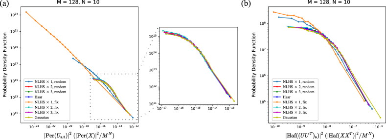
Figure 8: Probability density function for (a) FBS and (b) GBS with $M=128$ and $N=10$ each, for fixed (first $N$ modes over $M$ modes) and random input $\bm{t}$ and output $\bm{s}$ without collision. The distributions corresponding to the random NLHS circuit, with repetition numbers up to three, are presented. Also, the distributions of the Haar random matrices and random Gaussian matrices are displayed, to check if there exists the hiding property.

Appendix C Probability distributions of random NLHS circuit, for fixed mode number

To examine the scaling behavior of Haar measure convergence only in terms of photon number, we set mode number $M=32$ and photon number $N=8,16$, and sampled 10000 unitary matrices for each repetition of the random NLHS circuit and global Haar unitary circuit. Now we fix the input and output mode, as the photon number is comparably large such that the condition to get collision-free outcomes dominantly (i.e., $N=\mathcal{O}(\sqrt{M})$) may no longer hold. We calculate probabilities for fixed (first $N$ modes over $M$ modes) input and output and plot the probability density function for those values in Fig. 7. We find that the number of repetitions required to imitate the distribution of Haar unitary is insensitive to increasing photon number, even for the case that output photon number is comparably larger than $\mathcal{O}(\sqrt{M})$.

Appendix D Numerical evidence for hiding

The hiding theorem is necessary to prove the hardness of the classical simulation of BS; to simplify, the theorem states that hiding random output instances into random circuit instances is possible. More specifically, for the FBS case, the squared permanent of the $N\times N$ submatrices randomly chosen from $M\times M$ Haar random unitary matrices is very similar to the squared permanent of the random Gaussian matrices $X\sim\mathcal{N}(0,1)_{\mathbb{C}}^{N\times N}$ with normalization factor $\frac{1}{M^{N}}$, if $M=\omega(N^{5})$ is satisfied (conjectured that $M=\omega(N^{2})$ is enough) [2]. Also, Ref. [4] suggested hiding property for GBS; for equal squeezing input, the output probability distribution over Haar random circuit instances is similar to the squared hafnian of the product of random Gaussian matrices.

To gather numerical evidence about whether the hiding property holds for the random NLHS circuit, we compare the results between fixed and random input/output configurations over the random NLHS circuit instances and examine their converging behavior to the distribution of Haar random matrices. We also compare those results with the distribution from random Gaussian matrices, that is, $|\text{Per}(X)|^{2}/M^{N}$ with $X\sim\mathcal{N}(0,1)_{\mathbb{C}}^{N\times N}$ for FBS [2], and $|\text{Haf}(XX^{T})|^{2}/M^{N}$ with $X\sim\mathcal{N}(0,1)_{\mathbb{C}}^{N\times M}$ for GBS [4]; they are believed to be hard to additively estimate on average. If the results for fixed and random input/output are close enough to each other, and also close enough to the distributions of Haar random matrices and random Gaussian matrices, it gives evidence that hiding random output probabilities into average-case hard-to-estimate quantity (conjectured) would be possible.

We set mode number $M=128$ and photon number $N=10$, and sampled 10000 unitary matrices for each repetition of the random NLHS circuit. We calculate probabilities both for fixed and random input/output for those matrices, where we fixed input and output modes to the first $N$ modes over $M$ modes. Also, we calculate probabilities from 10000 Haar unitary matrices and random Gaussian matrices of size $N\times N$ ($N\times M$ for GBS). We plot the probability density function for those values, which can be checked in Fig. 8. We find that the result demonstrates the manifestation of the hiding property comparably after stacking the random NLHS circuit twice, which is consistent with previous results. Both fixed and random output probabilities of random NLHS circuit instances converge to the distributions of Haar random unitary and random Gaussian matrices, suggesting numerical evidence of hiding property at the low-depth regime.

References

- [1] John Preskill. Quantum computing in the nisq era and beyond. Quantum, 2:79, 2018.
- [2] Scott Aaronson and Alex Arkhipov. The computational complexity of linear optics. In Proceedings of the forty-third annual ACM symposium on Theory of computing, pages 333–342, 2011.
- [3] Craig S Hamilton, Regina Kruse, Linda Sansoni, Sonja Barkhofen, Christine Silberhorn, and Igor Jex. Gaussian boson sampling. Physical review letters, 119(17):170501, 2017.
- [4] Abhinav Deshpande, Arthur Mehta, Trevor Vincent, Nicolás Quesada, Marcel Hinsche, Marios Ioannou, Lars Madsen, Jonathan Lavoie, Haoyu Qi, Jens Eisert, et al. Quantum computational advantage via high-dimensional gaussian boson sampling. Science advances, 8(1):eabi7894, 2022.
- [5] Adam Bouland, Bill Fefferman, Chinmay Nirkhe, and Umesh Vazirani. On the complexity and verification of quantum random circuit sampling. Nature Physics, 15(2):159–163, 2019.
- [6] Frank Arute, Kunal Arya, Ryan Babbush, Dave Bacon, Joseph C Bardin, Rami Barends, Rupak Biswas, Sergio Boixo, Fernando GSL Brandao, David A Buell, et al. Quantum supremacy using a programmable superconducting processor. Nature, 574(7779):505–510, 2019.
- [7] Han-Sen Zhong, Hui Wang, Yu-Hao Deng, Ming-Cheng Chen, Li-Chao Peng, Yi-Han Luo, Jian Qin, Dian Wu, Xing Ding, Yi Hu, et al. Quantum computational advantage using photons. Science, 370(6523):1460–1463, 2020.
- [8] Han-Sen Zhong, Yu-Hao Deng, Jian Qin, Hui Wang, Ming-Cheng Chen, Li-Chao Peng, Yi-Han Luo, Dian Wu, Si-Qiu Gong, Hao Su, et al. Phase-programmable Gaussian boson sampling using stimulated squeezed light. Physical review letters, 127(18):180502, 2021.
- [9] Lars S Madsen, Fabian Laudenbach, Mohsen Falamarzi Askarani, Fabien Rortais, Trevor Vincent, Jacob FF Bulmer, Filippo M Miatto, Leonhard Neuhaus, Lukas G Helt, Matthew J Collins, et al. Quantum computational advantage with a programmable photonic processor. Nature, 606(7912):75–81, 2022.
- [10] Yu-Hao Deng, Yi-Chao Gu, Hua-Liang Liu, Si-Qiu Gong, Hao Su, Zhi-Jiong Zhang, Hao-Yang Tang, Meng-Hao Jia, Jia-Min Xu, Ming-Cheng Chen, et al. Gaussian boson sampling with pseudo-photon-number resolving detectors and quantum computational advantage. arXiv preprint arXiv:2304.12240, 2023.
- [11] Sergio Boixo, Sergei V Isakov, Vadim N Smelyanskiy, Ryan Babbush, Nan Ding, Zhang Jiang, Michael J Bremner, John M Martinis, and Hartmut Neven. Characterizing quantum supremacy in near-term devices. Nature Physics, 14(6):595–600, 2018.
- [12] Yulin Wu, Wan-Su Bao, Sirui Cao, Fusheng Chen, Ming-Cheng Chen, Xiawei Chen, Tung-Hsun Chung, Hui Deng, Yajie Du, Daojin Fan, et al. Strong quantum computational advantage using a superconducting quantum processor. Physical review letters, 127(18):180501, 2021.
- [13] A Morvan, B Villalonga, X Mi, S Mandrà, A Bengtsson, PV Klimov, Z Chen, S Hong, C Erickson, IK Drozdov, et al. Phase transition in random circuit sampling. arXiv preprint arXiv:2304.11119, 2023.
- [14] Guifré Vidal. Efficient classical simulation of slightly entangled quantum computations. Physical review letters, 91(14):147902, 2003.
- [15] Guifré Vidal. Efficient simulation of one-dimensional quantum many-body systems. Physical review letters, 93(4):040502, 2004.
- [16] Frank Verstraete, Juan J Garcia-Ripoll, and Juan Ignacio Cirac. Matrix product density operators: Simulation of finite-temperature and dissipative systems. Physical review letters, 93(20):207204, 2004.
- [17] John C Napp, Rolando L La Placa, Alexander M Dalzell, Fernando GSL Brandao, and Aram W Harrow. Efficient classical simulation of random shallow 2d quantum circuits. Physical Review X, 12(2):021021, 2022.
- [18] Abhinav Deshpande, Bill Fefferman, Minh C Tran, Michael Foss-Feig, and Alexey V Gorshkov. Dynamical phase transitions in sampling complexity. Physical review letters, 121(3):030501, 2018.
- [19] Haoyu Qi, Diego Cifuentes, Kamil Brádler, Robert Israel, Timjan Kalajdzievski, and Nicolás Quesada. Efficient sampling from shallow gaussian quantum-optical circuits with local interactions. Physical Review A, 105(5):052412, 2022.
- [20] Changhun Oh, Youngrong Lim, Bill Fefferman, and Liang Jiang. Classical simulation of boson sampling based on graph structure. Physical Review Letters, 128(19):190501, 2022.
- [21] Dorit Aharonov, Michael Ben-Or, Russell Impagliazzo, and Noam Nisan. Limitations of noisy reversible computation. arXiv preprint quant-ph/9611028, 1996.
- [22] Sergio Boixo, Vadim N Smelyanskiy, and Hartmut Neven. Fourier analysis of sampling from noisy chaotic quantum circuits. arXiv preprint arXiv:1708.01875, 2017.
- [23] Xun Gao and Luming Duan. Efficient classical simulation of noisy quantum computation. arXiv preprint arXiv:1810.03176, 2018.
- [24] Samson Wang, Enrico Fontana, Marco Cerezo, Kunal Sharma, Akira Sone, Lukasz Cincio, and Patrick J Coles. Noise-induced barren plateaus in variational quantum algorithms. Nature communications, 12(1):6961, 2021.
- [25] Abhinav Deshpande, Pradeep Niroula, Oles Shtanko, Alexey V Gorshkov, Bill Fefferman, and Michael J Gullans. Tight bounds on the convergence of noisy random circuits to the uniform distribution. PRX Quantum, 3(4):040329, 2022.
- [26] Gil Kalai and Guy Kindler. Gaussian noise sensitivity and bosonsampling. arXiv preprint arXiv:1409.3093, 2014.
- [27] Jelmer Renema, Valery Shchesnovich, and Raul Garcia-Patron. Classical simulability of noisy boson sampling. arXiv preprint arXiv:1809.01953, 2018.
- [28] Jelmer J Renema, Adrian Menssen, William R Clements, Gil Triginer, William S Kolthammer, and Ian A Walmsley. Efficient classical algorithm for boson sampling with partially distinguishable photons. Physical review letters, 120(22):220502, 2018.
- [29] Valery S Shchesnovich. Noise in boson sampling and the threshold of efficient classical simulatability. Physical Review A, 100(1):012340, 2019.
- [30] Alexandra E Moylett, Raúl García-Patrón, Jelmer J Renema, and Peter S Turner. Classically simulating near-term partially-distinguishable and lossy boson sampling. Quantum Science and Technology, 5(1):015001, 2019.
- [31] Daniel Jost Brod and Michał Oszmaniec. Classical simulation of linear optics subject to nonuniform losses. Quantum, 4:267, 2020.
- [32] Changhun Oh, Liang Jiang, and Bill Fefferman. On classical simulation algorithms for noisy boson sampling. arXiv preprint arXiv:2301.11532, 2023.
- [33] Changhun Oh, Minzhao Liu, Yuri Alexxev, Bill Fefferman, and Liang Jiang. Tensor network algorithm for simulating experimental gaussian boson sampling. arXiv preprint arXiv:2306.03709, 2023.
- [34] Michał Oszmaniec and Daniel J Brod. Classical simulation of photonic linear optics with lost particles. New Journal of Physics, 20(9):092002, 2018.
- [35] Raúl García-Patrón, Jelmer J Renema, and Valery Shchesnovich. Simulating boson sampling in lossy architectures. Quantum, 3:169, 2019.
- [36] Haoyu Qi, Daniel J Brod, Nicolás Quesada, and Raúl García-Patrón. Regimes of classical simulability for noisy gaussian boson sampling. Physical review letters, 124(10):100502, 2020.
- [37] Ramis Movassagh. Quantum supremacy and random circuits. arXiv preprint arXiv:1909.06210, 2019.
- [38] Yasuhiro Kondo, Ryuhei Mori, and Ramis Movassagh. Quantum supremacy and hardness of estimating output probabilities of quantum circuits. In 2021 IEEE 62nd Annual Symposium on Foundations of Computer Science (FOCS), pages 1296–1307. IEEE, 2022.
- [39] Adam Bouland, Bill Fefferman, Zeph Landau, and Yunchao Liu. Noise and the frontier of quantum supremacy. In 2021 IEEE 62nd Annual Symposium on Foundations of Computer Science (FOCS), pages 1308–1317. IEEE, 2022.
- [40] Michael J Bremner, Ashley Montanaro, and Dan J Shepherd. Average-case complexity versus approximate simulation of commuting quantum computations. Physical review letters, 117(8):080501, 2016.
- [41] Dominik Hangleiter, Juan Bermejo-Vega, Martin Schwarz, and Jens Eisert. Anticoncentration theorems for schemes showing a quantum speedup. Quantum, 2:65, 2018.
- [42] Juan Bermejo-Vega, Dominik Hangleiter, Martin Schwarz, Robert Raussendorf, and Jens Eisert. Architectures for quantum simulation showing a quantum speedup. Physical Review X, 8(2):021010, 2018.
- [43] Alexander M Dalzell, Nicholas Hunter-Jones, and Fernando GSL Brandão. Random quantum circuits anticoncentrate in log depth. PRX Quantum, 3(1):010333, 2022.
- [44] Boaz Barak, Chi-Ning Chou, and Xun Gao. Spoofing linear cross-entropy benchmarking in shallow quantum circuits. arXiv preprint arXiv:2005.02421, 2020.
- [45] Dorit Aharonov, Xun Gao, Zeph Landau, Yunchao Liu, and Umesh Vazirani. A polynomial-time classical algorithm for noisy random circuit sampling. arXiv preprint arXiv:2211.03999, 2022.
- [46] Leslie G Valiant. The complexity of computing the permanent. Theoretical computer science, 8(2):189–201, 1979.
- [47] Nicholas J Russell, Levon Chakhmakhchyan, Jeremy L O’Brien, and Anthony Laing. Direct dialling of haar random unitary matrices. New journal of physics, 19(3):033007, 2017.
- [48] Karol Zyczkowski and Marek Kus. Random unitary matrices. Journal of Physics A: Mathematical and General, 27(12):4235, 1994.
- [49] William R Clements, Peter C Humphreys, Benjamin J Metcalf, W Steven Kolthammer, and Ian A Walmsley. Optimal design for universal multiport interferometers. Optica, 3(12):1460–1465, 2016.
- [50] Bingzhi Zhang and Quntao Zhuang. Entanglement formation in continuous-variable random quantum networks. npj Quantum Information, 7(1):33, 2021.
- [51] Hao Tang, Xiao-Feng Lin, Zhen Feng, Jing-Yuan Chen, Jun Gao, Ke Sun, Chao-Yue Wang, Peng-Cheng Lai, Xiao-Yun Xu, Yao Wang, et al. Experimental two-dimensional quantum walk on a photonic chip. Science advances, 4(5):eaat3174, 2018.
- [52] Hao Tang, Leonardo Banchi, Tian-Yu Wang, Xiao-Wen Shang, Xi Tan, Wen-Hao Zhou, Zhen Feng, Anurag Pal, Hang Li, Cheng-Qiu Hu, et al. Generating haar-uniform randomness using stochastic quantum walks on a photonic chip. Physical Review Letters, 128(5):050503, 2022.
- [53] Douglass Stott Parker. Random butterfly transformations with applications in computational linear algebra. UCLA Computer Science Department, 1995.
- [54] Michael Mathieu and Yann LeCun. Fast approximation of rotations and hessians matrices. arXiv preprint arXiv:1404.7195, 2014.
- [55] Tri Dao, Albert Gu, Matthew Eichhorn, Atri Rudra, and Christopher Ré. Learning fast algorithms for linear transforms using butterfly factorizations. In International conference on machine learning, pages 1517–1527. PMLR, 2019.
- [56] Joseph Emerson, Yaakov S Weinstein, Marcos Saraceno, Seth Lloyd, and David G Cory. Pseudo-random unitary operators for quantum information processing. science, 302(5653):2098–2100, 2003.
- [57] Joseph Emerson, Etera Livine, and Seth Lloyd. Convergence conditions for random quantum circuits. Physical Review A, 72(4):060302, 2005.
- [58] Frank Verstraete and J Ignacio Cirac. Matrix product states represent ground states faithfully. Physical review b, 73(9):094423, 2006.
- [59] Norbert Schuch, Michael M Wolf, Frank Verstraete, and J Ignacio Cirac. Entropy scaling and simulability by matrix product states. Physical review letters, 100(3):030504, 2008.
- [60] Gerardo Adesso, Davide Girolami, and Alessio Serafini. Measuring gaussian quantum information and correlations using the rényi entropy of order 2. Physical review letters, 109(19):190502, 2012.
- [61] Ludovico Lami, Christoph Hirche, Gerardo Adesso, and Andreas Winter. Schur complement inequalities for covariance matrices and monogamy of quantum correlations. Physical Review Letters, 117(22):220502, 2016.
- [62] Giancarlo Camilo, Gabriel T Landi, and Sebas Eliëns. Strong subadditivity of the rényi entropies for bosonic and fermionic gaussian states. Physical Review B, 99(4):045155, 2019.
- [63] Joseph T Iosue, Adam Ehrenberg, Dominik Hangleiter, Abhinav Deshpande, and Alexey V Gorshkov. Page curves and typical entanglement in linear optics. arXiv preprint arXiv:2209.06838, 2022.
- [64] Alessio Serafini. Quantum continuous variables: a primer of theoretical methods. CRC press, 2017.
- [65] Andrea Crespi, Roberto Osellame, Roberta Ramponi, Marco Bentivegna, Fulvio Flamini, Nicolò Spagnolo, Niko Viggianiello, Luca Innocenti, Paolo Mataloni, and Fabio Sciarrino. Suppression law of quantum states in a 3d photonic fast fourier transform chip. Nature communications, 7(1):10469, 2016.
- [66] Poolad Imany, Navin B Lingaraju, Mohammed S Alshaykh, Daniel E Leaird, and Andrew M Weiner. Probing quantum walks through coherent control of high-dimensionally entangled photons. Science advances, 6(29):eaba8066, 2020.
- [67] Yaowen Hu, Christian Reimer, Amirhassan Shams-Ansari, Mian Zhang, and Marko Loncar. Realization of high-dimensional frequency crystals in electro-optic microcombs. Optica, 7(9):1189–1194, 2020.
- [68] Hoi-Kwan Lau and Daniel FV James. Proposal for a scalable universal bosonic simulator using individually trapped ions. Physical Review A, 85(6):062329, 2012.
- [69] Chao Shen, Zhen Zhang, and L-M Duan. Scalable implementation of boson sampling with trapped ions. Physical review letters, 112(5):050504, 2014.
- [70] Dietrich Leibfried, Rainer Blatt, Christopher Monroe, and David Wineland. Quantum dynamics of single trapped ions. Reviews of Modern Physics, 75(1):281, 2003.
- [71] Wentao Chen, Yao Lu, Shuaining Zhang, Kuan Zhang, Guanhao Huang, Mu Qiao, Xiaolu Su, Jialiang Zhang, Jing-Ning Zhang, Leonardo Banchi, et al. Scalable and programmable phononic network with trapped ions. Nature Physics, pages 1–7, 2023.
- [72] Alex Arkhipov. Bosonsampling is robust against small errors in the network matrix. Physical Review A, 92(6):062326, 2015.