Large deviations of homological growth rates
for hyperbolic surfaces

Abstract.

We perform a large deviations analysis of homological growth rates of oriented geodesics on hyperbolic surfaces. For surfaces uniformized by a wide class of Fuchsian groups of the first kind, we prove the existence of the rate function which estimates exponential probabilities with which the homological growth rates stay away from the mean value. The rate function is given in terms of the multifractal dimension spectrum described in our earlier result [12]. We also establish an Erdős-Rényi law, and refined large deviations upper bounds.

1. Introduction

Let $G$ denote a finitely generated, non-elementary Fuchsian group of the first kind acting on the Poincaré disc model $(\mathbb{D},d)$ of hyperbolic space. For each $g\in G$ let $|g|$ denote the minimal number of elements in a fixed set of generators needed to represent $g$, called the word length of $g$. There exists $\overline{\alpha}>0$ such that $d(0,g0)\leq\overline{\alpha}|g|$ for all $g\in G$. If $\mathbb{D}/G$ is compact, the Milnor-Swarc Lemma implies the existence of $\underline{\alpha}>0$ such that $d(0,g0)\geq\underline{\alpha}|g|$ for all $g\in G$. If $\mathbb{D}/G$ is non-compact, there exists $C>0$ such that $d(0,g0)\geq 2\log|g|-C$ for all $g\in G$ [11]. The complexity of the action of $G$ is reflected in the fact that the growth rate of $d(0,g0)/|g|$ as $|g|\rightarrow\infty$ takes on uncountably many values, and rates of convergence are not uniform. In this paper we perform a large deviations analysis of this growth rate along oriented geodesics.

Let $R\subset\mathbb{D}$ be a convex, locally finite fundamental domain for $G$ which contains $0$ in its interior [2]. The finite set of side-pairings of $R$, denoted by $G_{R}$, defines a symmetric set of generators of $G$. We assume $R$ is admissible, see Section 2.1 for the definition. Let $\mathscr{R}$ denote the set of oriented complete geodesics joining two points in $\mathbb{S}^{1}$ and intersecting the interior of $R$. If $\gamma\in\mathscr{R}$ cuts successively the copies $R,g_{0}R,g_{0}g_{1}R,\ldots$ of $R$, with $g_{i}\in G_{R}$ for $i=0,1,\ldots\in\mathbb{N}$, then $g_{0},g_{1},g_{2},\ldots$ is called the cutting sequence of $\gamma$ (see Figure 1). For each $\gamma\in\mathscr{R}$ whose positive endpoint $\gamma^{+}$ is contained in the conical limit set $\Lambda_{c}=\Lambda_{c}(G)$, an infinite cutting sequence $(g_{n})_{n=0}^{\infty}$ will be uniquely defined in Section 2.1. For each $n\geq 1$, the word length of $g_{0}\cdots g_{n-1}$ with respect to $G_{R}$ equals $n$ [22, Theorem 3.1(ii)]. We define

$$t_{n}(\gamma)=d(0,g_{0}g_{1}\cdots g_{n-1}0),$$

and call $t_{n}(\gamma)/n$ the homological growth rate of $\gamma$.

The set $\Lambda_{c}$ equals the complement of the countable set of fixed points of parabolic elements of $G$ [3], and the limit of the homological growth rates takes on uncountably many values. We put

$$\alpha_{+}=\sup_{\gamma\in\mathscr{R},\gamma^{+}\in\Lambda_{c}}\limsup_{n\to\infty}\frac{t_{n}(\gamma)}{n}\quad\text{and}\quad\alpha_{-}=\inf_{\gamma\in\mathscr{R},\gamma^{+}\in\Lambda_{c}}\liminf_{n\to\infty}\frac{t_{n}(\gamma)}{n},$$

and for each $\alpha\in[\alpha_{-},\alpha_{+}]$ define the level set

$$\mathscr{H}(\alpha)=\left\{\xi\in\Lambda_{c}\colon\text{there exists $\gamma\in\mathscr{R}$\ such that $\gamma^{+}=\xi$ and }\lim_{n\to\infty}\frac{t_{n}(\gamma)}{n}=\alpha\right\}.$$

With a slight abuse of notation, let $|$ $\cdot$ $|$ denote the Lebesgue measure on $\mathbb{S}^{1}$. In this paper we are concerned with the sets

$$\mathscr{H}_{n}(A)=\left\{\xi\in\Lambda_{c}\colon\exists\gamma\in\mathscr{R}\text{ s.t. }\gamma^{+}=\xi,\ \frac{t_{n}(\gamma)}{n}\in A\right\},$$

where $A\subset\mathbb{R}$ and $n\geq 1$, and interested in giving bounds on $|\mathscr{H}_{n}(A)|$. Put

$$\underline{\alpha}=\inf_{g\in G\setminus\{1\}}\frac{d(0,g0)}{|g|}\ \text{ and }\ \overline{\alpha}=\sup_{g\in G}\frac{d(0,g0)}{|g|}.$$

In fact we have $\underline{\alpha}=\alpha_{-}$ and $\overline{\alpha}=\alpha_{+}$ (see Theorem 2.5). Hence, $\mathscr{H}_{n}(A)\neq\emptyset$ implies $A\cap[\underline{\alpha},\overline{\alpha}]\neq\emptyset.$ By the Milnor-Swarc Lemma, $\underline{\alpha}>0$ holds if and only if $G$ has no parabolic element. There exists a constant $\alpha_{G}\in[\underline{\alpha},\overline{\alpha})$ (see (2.10) for the definition) such that $\mathscr{H}(\alpha_{G})$ has the full Lebesgue measure [12, Proposition A.8]. Hence, if $A$ is a closed set not containing $\alpha_{G}$ then $\lim_{n\to\infty}|\mathscr{H}_{n}(A)|=0$. Our result below asserts that the speed of this convergence is exponential, and the exponential rate is controlled by an analytic function.

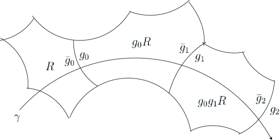
Figure 1. An oriented geodesic $\gamma$ crossing the copies of the fundamental domain $R$.

Theorem A.

Let $G$ be a finitely generated Fuchsian group of the first kind with an admissible fundamental domain. There exists a function $I\colon\mathbb{R}\to[0,+\infty]$ with the following properties:

• For any non-degenerate interval $A$ intersecting $(\underline{\alpha},\overline{\alpha})$ we have

  $$\lim_{n\to\infty}\frac{1}{n}\log\left|\mathscr{H}_{n}(A)\right|=-\inf_{\alpha\in A}I(\alpha).$$

• We have $I^{-1}(+\infty)=\mathbb{R}\setminus[\underline{\alpha},\overline{\alpha}]$, $I$ is continuous on $[\underline{\alpha},\overline{\alpha}]$, analytic on $(\underline{\alpha},\overline{\alpha})$, $I(\alpha_{G})=0$ and $I^{\prime\prime}>0$ on $(\underline{\alpha},\overline{\alpha})$. If $G$ has no parabolic element, then $\lim_{\alpha\searrow\underline{\alpha}}I^{\prime}(\alpha)=-\infty$ and $\lim_{\alpha\nearrow\overline{\alpha}}I^{\prime}(\alpha)=+\infty$. If $G$ has a parabolic element, then $\lim_{\alpha\searrow\underline{\alpha}}I^{\prime}(\alpha)=0$ and $\lim_{\alpha\nearrow\overline{\alpha}}I^{\prime}(\alpha)=+\infty$.

A function on $\mathbb{R}$ with the properties in Theorem A is called a rate function. Clearly, the rate function is unique. It is tightly linked to the multifractal dimension spectrum of homological growth rates analyzed in [12]. Let $\dim_{\rm H}$ denote the Hausdorff dimension on $\mathbb{S}^{1}$, and for $\alpha\in[\underline{\alpha},\overline{\alpha}]$ we set

$$b(\alpha)=\dim_{\rm H}\mathscr{H}(\alpha).$$

The function $\alpha\mapsto b(\alpha)$ is called the $\mathscr{H}$-spectrum [12]. As is evident from the proof of Theorem A, the rate function $I$ (see Figure 2) is given by

(1.1) $$I(\alpha)=\begin{cases}\alpha(1-b(\alpha))&\text{ for }\alpha\in[\underline{\alpha},\overline{\alpha}],\\ +\infty&\text{ for }\alpha\in\mathbb{R}\setminus[\underline{\alpha},\overline{\alpha}].\end{cases}$$

For any finitely generated Fuchsian group $G$ of the first kind, Bowen and Series [5] constructed a piecewise analytic Markov map $f\colon\mathbb{S}^{1}\to\mathbb{S}^{1}$ which is orbit equivalent to the action of $G$ on the limit set $\mathbb{S}^{1}$, now called the Bowen-Series map. Using hyperbolic geometry and a result of Series in [22], we show that $|t_{n}(\gamma)-\log|(f^{n})^{\prime}\gamma^{+}|$ is bounded from above by $2\log n+{\rm const.}$, see Propositions 2.2 and 2.4. This reduces the proof of Theorem A(a) to proving the level-1 Large Deviation Principle (LDP) for the Birkhoff averages of $-\log|f^{\prime}|$. For a general account on large deviations, including the meanings of level-1 and level-2, we refer the reader to the book of Ellis [10, Chapter 1].

Apart from special cases, the function $-\log|f^{\prime}|$ has discontinuities. To ‘hide’ them, we represent $f$ as a symbolic dynamics over a finite alphabet. We then show the level-1 LDP on this shift space (Proposition 3.1), and that $I$ in (1.1) is the rate function (Proposition 3.2). To identify the rate function and verify its properties as in Theorem A(b), we use our earlier results in [12] on the multifractal analysis of the homological growth rates.

The Markov partition for the Bowen-Series map $f$ constructed in [5] is an infinite partition if and only if $G$ has a parabolic element. If $G$ has no parabolic element, the Markov partition semiconjugates $f$ to a transitive finite Markov shift. The function $-\log|f^{\prime}|$ induces a Hölder continuous function on this shift space, and the level-2 LDP holds [16, 17, 23]. Via the contraction principle we obtain the desired level-1 LDP. It also follows directly from the estimates in [25].

If $G$ has a parabolic element, instead of the infinite Markov partition in [5] we use the finite Markov partition constructed in [12] that still semiconjugates $f$ to a transitive finite Markov shift. Although the function induced from $-\log|f^{\prime}|$ on this shift space is no longer Hölder continuous, one can still extend arguments in [23] to establish the level-2 LDP. Via the contraction principle we obtain the desired level-1 LDP.

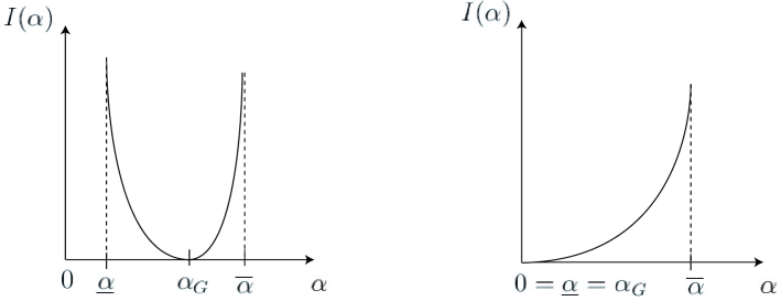
Figure 2. The graphs of the rate function $I$: $G$ has no parabolic element (left); $G$ has a parabolic element (right).

Theorem A has a further interesting consequence. If $G$ has no parabolic element, then $|t_{n}(\gamma)-\log|(f^{n})^{\prime}\gamma^{+}||$ is uniformly bounded (Proposition 2.4). Hence, combining Theorem A with [8, Proposition 2.2] we obtain the following statement.

Corollary 1.1 (An Erdős-Rényi law).

Let $G$ be a finitely generated Fuchsian group of the first kind without a parabolic element and with an admissible fundamental domain. For any $\alpha\in(\underline{\alpha},\overline{\alpha})$, for Lebesgue almost every $\xi\in\Lambda_{c}(G)$ and for any $\gamma\in\mathscr{R}$ with $\gamma^{+}=\xi$ we have

$$\lim_{n\to\infty}\max_{0\leq m\leq n-\lfloor\log n/I(\alpha)\rfloor}\frac{t_{m+\lfloor\log n/I(\alpha)\rfloor}(\gamma)-t_{m}(\gamma)}{\log n}=\frac{\alpha}{I(\alpha)}=\frac{1}{1-b(\alpha)}.$$

The $\mathscr{H}$-spectrum $\alpha\in[\underline{\alpha},\overline{\alpha}]\mapsto b(\alpha)$ encodes information on the complexity of the limit set. Although determined by rare events in the sense of the Lebesgue measure on $\Lambda_{c}$, the $\mathscr{H}$-spectrum can be computed from a single typical oriented geodesic as stated in Corollary 1.1. It is desirable to establish a similar formula for groups with parabolic elements.

Giving sharp bounds on $|\mathscr{H}_{n}(\cdot)|$ is more delicate. Suppose $G$ has no parabolic element. Combining the results in [7] [13, Korollar 5.8] with ours we obtain constants $0<c_{0}<c_{1}$ and $\varepsilon_{0}>0$ such that for $n\geq 1+|I^{\prime}(\alpha)|^{-4}$,

$$\frac{c_{0}e^{-I(\alpha)n}}{-I^{\prime}(\alpha)\sqrt{n}}\leq\mathscr{H}_{n}((-\infty,\alpha])\leq\frac{c_{1}e^{-I(\alpha)n}}{-I^{\prime}(\alpha)\sqrt{n}}\ \text{ for }\alpha\in(\alpha_{G}-\varepsilon_{0},\alpha_{G}),\text{ and }$$

$$\frac{c_{0}e^{-I(\alpha)n}}{I^{\prime}(\alpha)\sqrt{n}}\leq\mathscr{H}_{n}([\alpha,+\infty))\leq\frac{c_{1}e^{-I(\alpha)n}}{I^{\prime}(\alpha)\sqrt{n}}\ \text{ for }\alpha\in(\alpha_{G},\alpha_{G}+\varepsilon_{0}),$$

which are in agreement with the case of the sum of independently identically distributed random variables [1]. These sharp bounds were used in [7] to obtain convergence rates in the Erdős-Rényi law.

The methods in [7, 13] rely on a perturbation theory of transfer operators, and so those $\alpha$ not close to $\alpha_{G}$ are unaccounted for. We have obtained upper bounds which are weaker than [7, 13] for $\alpha$ close to $\alpha_{G}$ but valid for all $\alpha\in(\underline{\alpha},\overline{\alpha})\setminus\{0\}$. For sets $A\subset\mathbb{R}$, $K\subset\mathbb{D}$ and $n\geq 1$, let

$$\mathscr{H}_{n}(A,K)=\left\{\xi\in\Lambda_{c}\colon\exists\gamma\in\mathscr{R}\text{ s.t. }\gamma^{+}=\xi,\ \gamma\cap K\neq\emptyset,\ \frac{t_{n}(\gamma)}{n}\in A\right\}.$$

Theorem B.

Let $G$ be a finitely generated Fuchsian group of the first kind with an admissible fundamental domain.

• If $G$ has no parabolic element, then there exist constants $\kappa_{0}>0$, $\kappa_{1}>1$, $\kappa_{2}>1$ such that the following holds. For any $\alpha\in(\alpha_{G},\overline{\alpha})$ and any $n\geq\kappa_{0}/\alpha$ we have

  $$\left|\mathscr{H}_{n}([\alpha,+\infty))\right|\leq\kappa_{1}\kappa_{2}^{I^{\prime}(\alpha)}e^{-I(\alpha)n}.$$

  For any $\alpha\in(\underline{\alpha},\alpha_{G})$ and any $n\geq\kappa_{0}/\alpha$ we have

  $$\left|\mathscr{H}_{n}((-\infty,\alpha])\right|\leq\kappa_{1}\kappa_{2}^{-I^{\prime}(\alpha)}e^{-I(\alpha)n}.$$

• If $G$ has a parabolic element, then for any compact neighborhood $K$ of $0$ in $\mathbb{D}$ there exist constants $\kappa_{0}>0$, $\kappa_{1}>1$, $\kappa_{2}>1$ such that for any $\alpha\in(0,\overline{\alpha})$ and any $n\geq\max\{\kappa_{0}/\alpha,\min\left\{n\geq 1\colon(1/n)\log n\leq\alpha/3\right\}\}$ we have

  $$\left|\mathscr{H}_{n}([\alpha,+\infty),K)\right|\leq\kappa_{1}\kappa_{2}^{I^{\prime}(\alpha)}n^{2}e^{-I(\alpha)n}.$$

This type of upper bounds were obtained for the Gauss map [24], by extracting finite subsystems, applying to them the thermodynamic formalism [4, 20] and then using the regularity result of the Lyapunov spectrum [15, 18]. Our proof of Theorem B is an extension of the argument in [24] to the Bowen-Series maps, based on the regularity result of the $\mathscr{H}$-spectrum in [12]. Unlike the Gauss map, the Markov shift in the proof of Theorem A to which $f$ is semiconjugate is not the full shift. Hence, extracting finite subsystems is not straightforward. If $G$ has a parabolic element, it becomes more technical since $f$ has a neutral periodic point and a distortion control is necessary. To this end, we use the induced Markov map constructed in [12].

The rest of this paper consists of three sections. Section 2 provides preliminary results on the Fuchsian group actions and the Bowen-Series maps. We prove Theorem A in Section 3, and Theorem B in Section 4.

2. Preliminaries

This section provides preliminary results on Fuchsian groups and Bowen-Series maps. In Section 2.1 we give formal definitions of admissible fundamental domains and cutting sequences of oriented geodesics. In Section 2.2 we introduce the Bowen-Series map $f$. In Section 2.3 we prove key estimates comparing the homological growth rates and the growth rates of derivatives. After the definition of a Markov map in Section 2.4, we recall in Section 2.5 the construction of a finite Markov partition for $f$. In Section 2.6 we recall the results in [12] on the multifractal analysis of the homological growth rates.

2.1. Cutting sequences for fundamental domains with even corners

For $g\in G$, the inverse of $g$ is denoted by $\bar{g}$, and the word length of $g$ with respect to $G_{R}$ is denoted by $|g|$. Recall that $G_{R}$ is a symmetric set of generators of $G$: $g\in G_{R}$ implies $\bar{g}\in G_{R}$. Since $G$ is of the first kind, all the sides of $R$ are geodesics [19, Theorem 12.2.12]. Since $G$ is finitely generated, $R$ has finitely many sides.

The copies of $R$ adjacent to $R$ along the sides of $R$ are of the form $eR$, $e\in G_{R}$. For all $g\in G$ and $e\in G_{R}$, we label the side common to $gR$ and $geR$ on the side of $geR$ by $e$, and on the side of $gR$ by $\bar{e}$. By a side or vertex of $N=G\partial R$ we mean the $G$-image of a side or vertex of $R$. We say $R$ has even corners [5, 22] if $N$ is a union of complete geodesics. We say $R$ is admissible if $R$ has even corners with at least four sides and satisfies the following property: if $R$ has precisely four sides with all vertices in $\mathbb{D}$ then at least three geodesics in $N$ meet at each vertex of $R$ [22, Theorem 3.1]. The even corner assumption is not as restrictive as it appears: every surface which is uniformized by a finitely generated Fuchsian group has a fundamental domain with this property (see [5, Section 3] and [22, p.609, l.9-10]).

Unless otherwise stated we assume all geodesics are complete. If $\gamma\in\mathscr{R}$ passes through a vertex $v$ of $N$ in $\mathbb{D}$, we make the convention that $\gamma$ is replaced by a curve deformed to the right around $v$. We shall take as understood that all geodesics in $\mathscr{R}$ have been deformed, where necessary, in this way.

For $\gamma\in\mathscr{R}$ we define an infinite sequence $(g_{n})_{n=0}^{\infty}$ in $G_{R}$, called the cutting sequence of $\gamma$ as follows: $g_{0}$ is the exterior label of the side of $R$ across which $\gamma$ crosses from $R$ to $g_{0}R$, and for each $n\geq 1$, $g_{n}$ is the exterior label of the side of $g_{0}\cdots g_{n-1}R$ across which $\gamma$ crosses from $g_{0}\cdots g_{n-1}R$ to $g_{0}\cdots g_{n}R$.

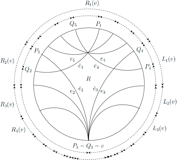
Figure 3. A fundamental domain $R$ of a finitely generated, non-free Fuchsian group of the first kind with four sides: $e_{1}$ and $e_{4}$, $e_{2}$ and $e_{3}$ are identified in pairs, which yields a non-compact hyperbolic surface of genus $0$ with one ramification point. The arcs in the inner dotted circle indicate elements of the finite Markov partition $(\varDelta(a))_{a\in S}$ constructed in Section 2.5.

2.2. The Bowen-Series map

Let $m$ denote the number of sides of the fundamental domain $R$, with exterior labels $e_{1},\ldots,e_{m}$ in anticlockwise order. For $1\leq i\leq m$ let $C(\bar{e}_{i})$ denote the Euclidean closure of the geodesic which contains the side of $R$ with exterior label $e_{i}$. We denote the two endpoints of $C(\bar{e}_{i})$ by $P_{i}$ and $Q_{i+1}$ in anticlockwise order. For $j\in\mathbb{Z}$ with $i=j$ mod $m$, set $e_{j}=e_{i}$, $P_{j}=P_{i}$, $Q_{j}=Q_{i}$. According to [5, 22], the Bowen-Series map $f\colon\mathbb{S}^{1}\to\mathbb{S}^{1}$ is given by

$$f|_{[P_{i},P_{i+1})}(x)=\bar{e}_{i}x.$$

For each $i\in\mathbb{Z}$, the restriction of $f$ to $(P_{i},P_{i+1})$ is analytic and can be extended to a $C^{\infty}$ map on $[P_{i},P_{i+1}]$. The derivatives of $f$ at points $P_{i}$ are the appropriate one-sided derivatives. If $P_{i}$ is a cusp, then it is a neutral periodic point of $f$.

Remark 2.1.

Unlike [5], we do not assume that $C(\bar{e}_{i})$ is contained in the isometric circle of $\bar{e}_{i}$. This means that the useful condition $\inf_{\mathbb{S}^{1}}|f^{\prime}|\geq 1$ may not hold.

The $f$-expansion of a point $\xi\in\mathbb{S}^{1}$ is the one-sided infinite sequence $\xi_{f}=(e_{i_{n}})_{n=0}^{\infty}\in G_{R}^{\mathbb{N}}$ given by $f^{n}(\xi)\in[P_{i_{n}},P_{i_{n}+1})$ for $n\geq 0.$ We will denote the $f$-expansion of $\xi\in\mathbb{S}^{1}$ by $(a_{n})_{n=0}^{\infty}\in G_{R}^{\mathbb{N}}$ to make a notational distinction from cutting sequences of geodesics. Note that $\overline{a_{0}\cdots a_{n-1}}\xi=f^{n}(\xi)$.

2.3. Comparing homological growth rates and growth of derivatives

For the rest of the paper, we assume $G$ has an admissible fundamental domain $R$, and $f$ is the associated Bowen-Series map.

Proposition 2.2.

Assume that $G$ has no parabolic element. There exists a constant $C_{0}>0$ such that for each geodesic $\gamma\in\mathscr{R}$ with the infinite cutting sequence $(g_{n})_{n=0}^{\infty}$ we have

$$\left|t_{n}(\gamma)-\log\left|(\overline{g_{0}\cdots g_{n-1}})^{\prime}\gamma^{+}\right|\right|\leq C_{0}\ \text{ and }\ |t_{n}(\gamma)-\log|(f^{n})^{\prime}\gamma^{+}||\leq C_{0}.$$

We introduce key ingredients for a proof of Proposition 2.2. The Busemann function is a function of $\xi\in\mathbb{S}^{1}$ and $a,b\in\mathbb{D}$ given by

$$B_{\xi}(a,b)=\lim_{t\rightarrow+\infty}\left(d(a,\gamma(t))-d(b,\gamma(t))\right),$$

where $\gamma=\{\gamma(t)\}_{t\in\mathbb{R}}$ is an oriented geodesic with $d(\gamma(s),\gamma(t))=|s-t|$ for $s,t\in\mathbb{R}$ whose positive endpoint is $\xi$. The limit always exists and is independent of the choice of $\gamma$. The Poisson kernel is a function of $x\in\mathbb{D}$ and $\xi\in\mathbb{S}^{1}$ given by

$$P(x,\xi)=\frac{1-|x|^{2}}{|\xi-x|^{2}}.$$

It is well known that (see [6, Example 8.24])

(2.1) $$B_{\gamma^{+}}(0,b)=\log P(b,\gamma^{+})=|\tau^{\prime}(\gamma^{+})|,$$

where $\tau$ is a Möbius transformation preserving $\mathbb{D}$ and satisfying $\tau(b)=0$.

If $G$ is a free group, the cutting sequence of $\gamma\in\mathscr{R}$ coincides with the $f$-expansion of $\gamma^{+}$, and so $(\overline{g_{0}\cdots g_{n-1}})^{\prime}\gamma^{+}=(f^{n})^{\prime}\gamma^{+}.$ If $G$ is not a free group, this is not always the case. The next lemma implies that the cutting sequence of $\gamma\in\mathscr{R}$ and the $f$-expansion of $\gamma^{+}$ differ only slightly.

Lemma 2.3 ([12] Lemma 2.7).

Let $\gamma\in\mathscr{R}$ have the infinite cutting sequence $(g_{n})_{n=0}^{\infty}$ and let $(a_{n})_{n=0}^{\infty}$ be the $f$-expansion of $\gamma^{+}$. For any $n\geq 0$, $g_{0}\cdots g_{n}R$ and $a_{0}\cdots a_{n}R$ share a common side of $N$, or else share a common vertex of $N$ in $\mathbb{D}$.

Proof of Proposition 2.2.

For $n\geq 1$ we put $x_{n}=g_{0}\cdots g_{n-1}0$. Since $G$ has no parabolic element, $R$ has a finite hyperbolic diameter, denoted by ${\rm diam}_{\rm h}(R)$. Put $C_{0}=4{\rm diam}_{\rm h}(R)$. It follows that for all $n\in\mathbb{N}$,

(2.2) $$\min\{d(x_{n},y)\colon y\in\gamma\}\leq\frac{C_{0}}{4}.$$

We denote by $p_{n}$ the intersection of $\gamma$ and the horocircle at $\gamma^{+}$ through $x_{n}$. Clearly, (2.2) together with the triangle inequality implies

(2.3) $$d(x_{n},p_{n})\leq\frac{C_{0}}{2}.$$

Fix $p_{0}\in\gamma\cap R$. By combining (2.3) with the triangle inequality and the fact that $B_{\gamma^{+}}(p_{0},x_{n})=d(p_{0},p_{n})$, we obtain

$$\begin{split}\left|d(0,x_{n})-B_{\gamma^{+}}(0,x_{n})\right|\leq&|d(0,x_{n})-d(p_{0},x_{n})|+|d(p_{0},x_{n})-d(p_{0},p_{n})|\\ &+|B_{\gamma^{+}}(p_{0},x_{n})-B_{\gamma^{+}}(0,x_{n})|\leq C_{0}.\end{split}$$

The first assertion follows from this and (2.1) with $b=x_{n}$. The second one follows from the same argument, replacing $g_{0}\cdots g_{n-1}$ by $a_{0}\cdots a_{n-1}$ and using the uniform bound on $d(x_{n},a_{0}\cdots a_{n-1}0)$ guaranteed by Lemma 2.3. ∎

Proposition 2.4.

Assume that $G$ has a parabolic element. Let $K$ be a compact neighborhood of $0$ in $\mathbb{D}$. There exists a constant $C_{0}>0$ such that for each geodesic $\gamma\in\mathscr{R}$ which intersects $K\cap R$ and has an infinite cutting sequence $(g_{n})_{n=0}^{\infty}$ we have

$$\left|t_{n}(\gamma)-\log\left|(\overline{g_{0}\cdots g_{n-1}})^{\prime}\gamma^{+}\right|\right|\leq 2\log n+C_{0},\text{ and}$$

$$|t_{n}(\gamma)-\log|(f^{n})^{\prime}\gamma^{+}||\leq 2\log n+C_{0}.$$

Proof.

By passing to an iterate of $f$, we may assume that all cusps of $R$ are fixed points of $f$. We follow the argument in [14, p.161 (3)]. Let $r_{0}>1$ be a large number to be determined later. For each cusp of $R$, we conjugate the cusp to infinity in the upper half-plane model and $0$ to $i$. For each cusp, we remove from $R$ the horodisk $H(r_{0})=\{z\in\mathbb{C}\colon{\rm Im}(z)>r_{0}\}$. This defines a compact subset $K(r_{0})$ of $R$. We take $r_{0}$ large enough so that $K\subset K(r_{0})$ and the horodisks associated with the cusps are pairwise disjoint.

For $n\geq 1$ we put $x_{n}=g_{0}\cdots g_{n-1}0$, and denote by $p_{n}$ the intersection of $\gamma$ and the horocircle at $\gamma^{+}$ through $x_{n}$. First assume that $\gamma\cap g_{0}\cdots g_{n-1}(R\cap K(r_{0}))$ is non-empty. Then $\gamma$ passes within the distance ${\rm diam_{\rm h}}(K(r_{0}))$ of $x_{n}$, which implies

(2.4) $$d(x_{n},p_{n})\leq 2{\rm diam_{\rm h}}(K(r_{0})).$$

Now assume that $\gamma\cap g_{0}\cdots g_{n-1}(R\cap K(r_{0}))$ is empty. Then $\gamma\cap g_{0}\cdots g_{n-1}R$ is contained in one of the horodisks that are the $g_{0}\cdots g_{n-1}$-images of the horodisks removed from $R$. Conjugating the $g_{0}\cdots g_{n-1}$-image of the cusp in this horodisk to infinity in the upper half-plane model and $x_{n}$ to $i$ we see that $\gamma\cap g_{0}\cdots g_{n-1}R\subset H(r_{0})$. Let $m\leq n$ denote the smallest integer such that for all $k\in\{m,m+1,\ldots,n\}$ we have $\gamma\cap g_{0}\cdots g_{k-1}R\subset H(r_{0})$. Since the cusp is a fixed point of $f$, we have $x_{k}=i+(n-k)\lambda$ for all $k\in\{m,m+1,\ldots,n\}$, with some $\lambda\in\mathbb{R}\setminus\{0\}$ depending only on the cusp. Let $x^{\prime}$ denote the unique point on $\gamma$ which satisfies ${\rm Re}(x^{\prime})<0$ and ${\rm Im}(x^{\prime})=1$ (see Figure 4). There exists a uniform constant $C^{\prime}=C^{\prime}(r_{0},\lambda)>0$ such that $d(x_{m},x^{\prime})\leq C^{\prime}$. Hence, there exists a constant $C^{\prime\prime}=C^{\prime\prime}(r_{0},\lambda)>0$ such that $|x_{m}-x^{\prime}|\leq C^{\prime\prime}$.

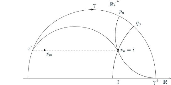
Figure 4. On the proof of Proposition 2.4 in the case $\gamma\cap g_{0}\cdots g_{n-1}(R\cap K(r_{0}))=\emptyset$ and $\lambda>0$.

We verify the existence of a constant $C=C(r_{0},\lambda)>0$ such that

(2.5) $$d(x^{\prime},x_{n})\leq 2\log(n-m)+C.$$

Let $r>1$ denote the Euclidean radius of the geodesic arc between $x^{\prime}$ and $x_{n}$. Then

$$d(x^{\prime},x_{n})=2\log(\sqrt{r^{2}-1}+r)$$

by [11]. Hence, for $r$ sufficiently large, $d(x^{\prime},x_{n})\leq 2\log(2\sqrt{r^{2}-1}+1)$. By the Euclidean Pythagorean theorem we have

$$2\sqrt{r^{2}-1}=|x^{\prime}-x_{n}|\leq|x^{\prime}-x_{m}|+|x_{m}-x_{n}|\leq|\lambda|(n-m)+C^{\prime\prime}.$$

Taking $C=2\log|\lambda|+2\log\left(1+(C^{\prime\prime}+1)/|\lambda|\right)$ we obtain

$$d(x^{\prime},x_{n})\leq 2\log(|\lambda|(n-m)+C^{\prime\prime}+1)\leq 2\log(n-m)+C.$$

This proves (2.5) for all $r$ sufficiently large. Enlarging $C$ if necessary, we can show (2.5) for all $r>1$. The proof of (2.5) is complete.

Let $q_{n}$ denote the point of intersection between $\gamma$ and the geodesic through $x_{n}$ that is orthogonal to $\gamma$ (see Figure 4). Since the hyperbolic triangle with vertices $x^{\prime}$, $x_{n}$, $q_{n}$ has a right angle at $q_{n}$, the hyperbolic Pythagorean theorem implies $d(x_{n},q_{n})<d(x^{\prime},x_{n})+2\log 2$. By (2.5) it follows that

(2.6) $$\begin{split}d(x_{n},p_{n})<d(x_{n},q_{n})&<d(x^{\prime},x_{n})+2\log 2\\ &\leq 2\log(n-m)+C+2\log 2\\ &\leq 2\log n+C+2\log 2.\end{split}$$

Proceeding exactly as in the proof of Proposition 2.2 replacing (2.3) by (2.4) and (2.6), we obtain the first desired estimate in Proposition 2.4. For the second one, we proceed in the same way replacing $g_{0}\cdots g_{n-1}$ by $a_{0}\cdots a_{n-1}$ and using $g_{k}=a_{k}$ for $m\leq k\leq n$ and Lemma 2.3. ∎

2.4. Markov maps

Let $S$ be a discrete set with $\#S\geq 2$. Given a set $\Sigma$ of one-sided infinite sequences $(x_{n})_{n=0}^{\infty}=x_{0}x_{1}\cdots$ in the cartesian product topological space $S^{\mathbb{N}}$, let $E(\Sigma)$ denote the set of finite words in $S$ that appear in some element of $\Sigma$. For an integer $n\geq 1$, let $E^{n}(\Sigma)$ denote the set of elements of $E(\Sigma)$ with word length $n$.

A Markov map is a map $F\colon\Gamma\to\mathbb{S}^{1}$ such that the following holds:

• There exists a family $(\Gamma(a))_{a\in S}$ of pairwise disjoint arcs in $\mathbb{S}^{1}$ such that $\Gamma=\bigcup_{a\in S}\Gamma(a)$.

• For each $a\in S$, the restriction $F|_{\Gamma(a)}$ extends to a $C^{1}$ diffeomorphism from the closure of $\Gamma(a)$ onto its image.

• If $a,b\in S$ and $F(\Gamma(a))\cap\Gamma(b)$ has non-empty interior, then $F(\Gamma(a))\supset\Gamma(b)$.

The family $(\Gamma(a))_{a\in S}$ of arcs is called a Markov partition of $F$.

Condition (iii) determines a transition matrix $(M_{ab})$ over the countable alphabet $S$ given by $M_{ab}=1$ if $F(\Gamma(a))\supset\Gamma(b)$ and $M_{ab}=0$ otherwise. It determines a countable topological Markov shift $\Sigma=\Sigma(F,(\Gamma(a))_{a\in S})$ by

(2.7) $$\Sigma=\{x=(x_{n})_{n=0}^{\infty}\in S^{\mathbb{N}}\colon M_{x_{n}x_{n+1}}=1\ \text{for }n\geq 0\}.$$

The relative topology on $\Sigma$ has a base that consists of sets of the form

$$[\omega_{0}\cdots\omega_{n-1}]=\{x\in\Sigma\colon x_{k}=\omega_{k}\ \text{for }0\leq k\leq n-1\},\ n\geq 1,\ \omega_{0}\cdots\omega_{n-1}\in S^{n}.$$

This topology is metrizable with the metric $d_{\Sigma}$ given by $d_{\Sigma}(x,y)=\exp(-\min\{n\geq 0\colon x_{n}\neq y_{n}\})$ for distinct points $x,y\in\Sigma$.

If $\bigcap_{n=0}^{\infty}\overline{F^{-n}(\Gamma(x_{n}))}$ is a singleton for all $(x_{n})_{n=0}^{\infty}\in\Sigma$, then we define a coding map $\pi_{\Sigma}\colon\Sigma\to\mathbb{S}^{1}$ by

(2.8) $$\pi_{\Sigma}((x_{n})_{n=0}^{\infty})\in\bigcap_{n=0}^{\infty}\overline{F^{-n}(\Gamma(x_{n}))}.$$

The coding map is continuous and semiconjugates $F$ to the left shift on $\Sigma$.

For $\omega\in S^{m}$ and $\zeta\in S^{n}$, write $\omega\zeta$ for the concatenation $\omega_{0}\cdots\omega_{m-1}\zeta_{0}\cdots\zeta_{n-1}\in S^{m+n}$. For convenience, put $E^{0}=\{\emptyset\}$, $|\emptyset|=0$, and $\omega\emptyset=\omega=\emptyset\omega$ for all $\omega\in E(\Sigma)$.

2.5. Construction of a finite Markov partition

A point $v\in\mathbb{S}^{1}$ is called a cusp of $R$ if $v$ is the common endpoint of two sides of $R$. The set of all cusps of $R$ is denoted by $V_{c}$. Each cusp is a fixed point of some parabolic element of $G$. If $G$ has a parabolic element, then $V_{c}$ is non-empty.

Let $V$ denote the set of all vertices of $R$ in $\mathbb{D}\cup\mathbb{S}^{1}$. For each $v\in V$ we denote by $W(v)\subset\mathbb{S}^{1}$ the set of points where the geodesics in $N$ passing through $v$ meet $\mathbb{S}^{1}$. The set $\bigcup_{v\in V}W(v)$ is $f$-invariant [5, Lemma 2.3] and hence induces a Markov partition for $f$. This partition is an infinite partition if and only if $R$ has a cusp. If $R$ has a cusp, below we construct a coarser finite Markov partition for $f$ that determines a transitive finite Markov shift.

Let $v\in V_{c}$. There exists $i\in\mathbb{Z}$ such that $v\in C(\bar{e}_{i-1})\cap C(\bar{e}_{i})$. We denote the arcs of $\mathbb{S}^{1}$ cut-off by successive points of $W(v)$ in clockwise order from $Q_{i+1}$ to $Q_{i}=v$ as $L_{1}(v),L_{2}(v),\ldots$, and anticlockwise from $Q_{i+1}$ to $Q_{i}$ by $R_{1}(v),R_{2}(v),\ldots$, as in Figure 3. We define

$$L(v)=\overline{\bigcup_{r\geq 2}L_{r}(v)}\quad\text{and}\quad R(v)=\overline{\bigcup_{r\geq 3}R_{r}(v)}.$$

For each $v\in V$ we define

$$W^{\prime}(v)=\begin{cases}W(v)&\text{if $v\notin V_{c}$,}\\ \partial L_{1}(v)\cup\partial L(v)\cup\partial R_{2}(v)\cup\partial R(v)&\text{if $v\in V_{c}$,}\end{cases}$$

and put

$$W^{\prime}=\bigcup_{v\in V}W^{\prime}(v).$$

Note that $W^{\prime}$ is a finite subset of $\bigcup_{v\in V}W(v)$. One verifies $f(W^{\prime})\subset W^{\prime}$ [12, Lemma 3.1]. We define a partition of $\mathbb{S}^{1}$ into arcs with endpoints given by two consecutive points in $W^{\prime}$. We choose all partition elements to be left-closed and right-open, in anticlockwise order. We label the partition elements by integers from a finite subset $S$ of $\mathbb{N}$, and denote the partition element labeled with $a\in S$ by $\varDelta(a)$.

Then $f\colon\mathbb{S}^{1}\to\mathbb{S}^{1}$ is a Markov map with a finite Markov partition $(\varDelta(a))_{a\in S}$ (see [12, Proposition 3.2]), and determines by (2.7) a transitive finite Markov shift

$$X=X(f,(\varDelta(a))_{a\in S}).$$

By [12, Lemma 2.5], the coding map $\pi_{X}$ is well defined by (2.8). Let $\sigma\colon X\rightarrow X$ denote the left shift given by $(\sigma x)_{n}=x_{n+1}$ for $n\geq 0$. We have

$$f\circ\pi_{X}=\pi_{X}\circ\sigma.$$

2.6. Multifractal analysis of homological growth rates

Let $Y$ be a topological space and let $F\colon Y\to Y$ be a Borel map. Let $\mathcal{M}(Y)$ denote the space of $F$-invariant Borel probbility measures endowed with the weak* topology, and let $\mathcal{M}(Y,F)$ denote the set of elements of $\mathcal{M}(Y)$ which are invariant under $F$. For each $\mu\in\mathcal{M}(Y,F)$, let $h_{\mu}(F)$ denote the measure-theoretic entropy of $\mu$ with respect to $F$. If the dependence on $F$ is clear, we often write $h(\mu)$ for $h_{\mu}(F)$. For $\mu\in\mathcal{M}(\mathbb{S}^{1},f)$, we define the Lyapunov exponent of $\mu$ by $\chi(\mu)=\int\log|f^{\prime}|d\mu.$

Imitating the style of the Poincaré exponent, for each $\beta\in\mathbb{R}$ we define

$$P(\beta)=\inf\left\{t\in\mathbb{R}\colon\sum_{g\in G}\exp(-\beta d(0,g0)-t|g|)<+\infty\right\},$$

and call the function $\beta\in\mathbb{R}\mapsto P(\beta)$ a pressure function. Define

$$\beta_{+}=\sup\{\beta\in\mathbb{R}\colon P(\beta)>-\underline{\alpha}\beta\}.$$

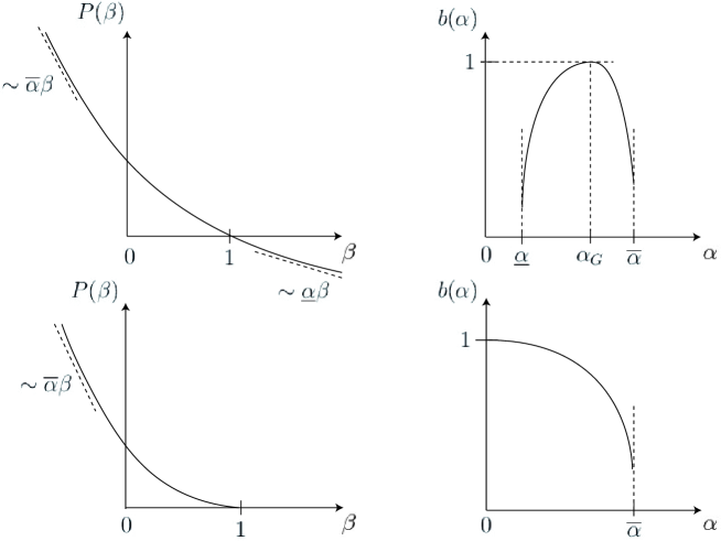
Figure 5. The graphs of the pressure function $\beta\in\mathbb{R}\mapsto P(\beta)$ and the $\mathscr{H}$-spectrum $\alpha\in[\underline{\alpha},\overline{\alpha}]\mapsto b(\alpha)$: $G$ has no parabolic element (upper); $G$ has a parabolic element (lower).

Theorem 2.5.

Let $G$ be a finitely generated non-elementary Fuchsian group of the first kind with an admissible fundamental domain $R$ having even corners.

• We have $\underline{\alpha}=\alpha_{-}$ and $\overline{\alpha}=\alpha_{+}$.

• The pressure function $P$ is convex, non-increasing and continuously differentiable on $\mathbb{R}$, and analytic and strictly convex on $(-\infty,\beta_{+})$. If $G$ has no parabolic element, then $\beta_{+}=+\infty$. If $G$ has a parabolic element, then $\beta_{+}=1$ and $P$ vanishes on $[1,+\infty).$

• We have $\underline{\alpha}<\overline{\alpha}$, and the level set $\mathscr{H}(\alpha)$ is non-empty if and only if $\alpha\in[\underline{\alpha},\overline{\alpha}]$. The $\mathscr{H}$-spectrum is continuous on $[\underline{\alpha},\overline{\alpha}]$, analytic on $(\underline{\alpha},\overline{\alpha})$, and for each $\alpha\in[\underline{\alpha},\overline{\alpha}]\setminus\{0\}$ we have

  (2.9) $$b(\alpha)=\max\left\{\frac{h(\mu)}{\chi(\mu)}\colon\mu\in\mathcal{M}(\mathbb{S}^{1},f),\ \chi(\mu)=\alpha\right\}.$$

  Moreover, the $\mathscr{H}$-spectrum attains its maximum $1$ at $\alpha_{G}\in[\underline{\alpha},\overline{\alpha})$, is strictly increasing on $[\underline{\alpha},\alpha_{G}]$ and strictly decreasing on $[\alpha_{G},\overline{\alpha}]$, where

  (2.10) $$\alpha_{G}=-P^{\prime}(1),$$

  and $\lim_{\alpha\nearrow\overline{\alpha}}b^{\prime}(\alpha)=-\infty$. If $G$ has no parabolic element, then $\alpha_{G}>\underline{\alpha}>0$ and $\lim_{\alpha\searrow\underline{\alpha}}b^{\prime}(\alpha)=+\infty$. If $G$ has a parabolic element, then $\alpha_{G}=\underline{\alpha}=0$.

Schematic graphs of the pressure and the $\mathscr{H}$-spectrum are shown in Figure 5.

To proceed, we need the following distortion property. Let $\Sigma^{+}$ denote the set of $f$-expansions of points in $\mathbb{S}^{1}$. Let $n\geq 1$ and let $a_{0}\cdots a_{n-1}\in E^{n}(\Sigma^{+})$. We define

$$\Theta(a_{0}\cdots a_{n-1})=\left\{\xi\in\mathbb{S}^{1}\colon f^{k}(\xi)\in[P_{i_{k}},P_{i_{k}+1})\quad\text{for }0\leq k\leq n-1\right\},$$

where $a_{k}=e_{i_{k}}\in G_{R}$ for $0\leq k\leq n-1$. Define

$$D_{n}=\sup_{a_{0}\cdots a_{n-1}\in E^{n}(\Sigma^{+})}\sup_{x,y\in\Theta(a_{0}\cdots a_{n-1})}\frac{|(f^{n})^{\prime}x|}{|(f^{n})^{\prime}y|}.$$

Proposition 2.6 ([12] Proposition 2.8).

We have $\log D_{n}=o(n)$ $(n\to\infty)$.

Remark 2.7.

If $G$ has no parabolic element, some power of $f$ is uniformly expanding [21, Theorem 5.1], and so $D_{n}$ is uniformly bounded. If $G$ has a parabolic element, Lemma 2.3 and Proposition 2.4 imply $D_{n}=O(n^{4})$. If moreover $\inf_{\mathbb{S}^{1}}|f^{\prime}|\geq 1$, then using the explicit form of parabolic elements in [5, Lemma 2.7] one can show that $D_{n}=O(n^{2})$.

Proof of Theorem 2.5.

Below we only prove (a) using the finite Markov partition constructed in Section 2.5. The rest of the assertions are contained in [12, Main Theorem, Proposition 5.3].

Since cutting sequences are shortest [22, Theorem 3.1(ii)], we have $\underline{\alpha}\leq\alpha_{-}$. To show the reverse inequality, take a sequence $(g_{n})_{n=1}^{\infty}$ in $G\setminus\{1\}$ such that $k$, $n\geq 1$, $k\neq n$ implies $g_{k}\neq g_{n}$, and for all $n\geq 1$,

(2.11) $$0\leq\frac{d(0,g_{n}0)}{|g_{n}|}-\underline{\alpha}<\frac{1}{n}.$$

Since $G$ is finitely generated, we have $|g_{n}|\to\infty$ as $n\to\infty$. Let $a_{n,0}\cdots a_{n,|g_{n}|-1}\in E^{|g_{n}|}(\Sigma^{+})$ denote the admissible shortest representation of $g_{n}$ (see [12, Lemma 3.9]). By the mean value theorem, there exists $C\geq 1$ such that for all $\xi\in\Theta(a_{n,0}\cdots a_{n,|g_{n}|-1})$ we have

(2.12) $$\frac{1}{CD_{n}}\leq\frac{|\Theta(a_{n,0}\cdots a_{n,|g_{n}|-1})|}{|(f^{|g_{n}|})^{\prime}\xi|^{-1}}\leq CD_{n}.$$

Pick $\omega_{0}\cdots\omega_{|g_{n}|-1}\in E^{|g_{n}|}(X)$ such that $\varDelta(\omega_{0}\cdots\omega_{|g_{n}|-1})\subset\Theta(a_{n,0}\cdots a_{n,|g_{n}|-1})$. Since $X$ is a transitive finite Markov shift, there is an integer $L\geq 1$ such that for each $n\geq 1$ there is a periodic point $\xi_{n}\in\varDelta(\omega_{0}\cdots\omega_{|g_{n}|-1})$ of period in $\{|g_{n}|,\ldots,|g_{n}|+L\}$. Let $\mu_{n}$ denote the uniform probability distribution on the $f$-orbit of $\xi_{n}$.

From the proof of [12, Proposition 2.9], there exists $C^{\prime}\geq 1$ such that

(2.13) $$\frac{1}{C^{\prime}}\leq\frac{|\Theta(a_{n,0}\cdots a_{n,|g_{n}|-1})|}{\exp(-d(0,a_{n,0}\cdots a_{n,|g_{n}|-1}0))}\leq C^{\prime}D_{|g_{n}|}.$$

Combining (2.11) and (2.12) with (2.13) and using Proposition 2.6 implies $\underline{\alpha}\geq\limsup_{n}\chi(\mu_{n})$. Since $\alpha_{-}=\inf\{\chi(\mu)\colon\mu\in\mathcal{M}(\mathbb{S}^{1},f)\}$ by [12, Lemma 3.6], we have $\limsup_{n}\chi(\mu_{n})\geq\alpha_{-}$. We have verified $\underline{\alpha}=\alpha_{-}$. The proof of $\overline{\alpha}=\alpha_{+}$ is analogous, with $\alpha_{+}=\sup\{\chi(\mu)\colon\mu\in\mathcal{M}(\mathbb{S}^{1},f)\}$ also by [12, Lemma 3.6]. ∎

3. Large deviations

This section is dedicated to the proof of Theorem A. In Section 3.1 we prove the level-1 LDP on the shift space $X$, and in Section 3.2 we prove that the rate function is $I$. In Section 3.3 we complete the proof of Theorem A.

3.1. Large deviations on the shift space of finite type

From the proof of Ruelle’s Perron-Frobenius theorem in [4], there exists a Borel probability measure $m$ on $X$ and a constant $C\geq 1$ such that for $\omega\in X$ and $n\geq 1$,

(3.1) $$\frac{1}{CD_{n}}\leq\frac{m[\omega_{0}\cdots\omega_{n-1}]}{\exp\sum_{k=0}^{n-1}\varphi(\sigma^{k}\omega)}\leq CD_{n}.$$

Here, we have used that $P(1)=0$, which follows from our assumption that $G$ is of the first kind and Bowen’s formula [12, Proposition 5.4].

Note that the function

(3.2) $$\varphi=-\log|f^{\prime}|\circ\pi_{X}$$

is continuous, although $-\log|f^{\prime}|$ may have discontinuities. We define the convex rate function $I_{\varphi}\colon\mathbb{R}\to[0,+\infty]$ by

$$I_{\varphi}(\alpha)=-\sup\left\{h(\mu)+\int\varphi d\mu\colon\mu\in\mathcal{M}(X,\sigma),-\int\varphi d\mu=\alpha\right\}.$$

Since $X$ is a finite shift space, the entropy map is upper semicontinuous. Hence, $I_{\varphi}$ is lower semicontinuous.

Proposition 3.1 (Level-1 LDP).

For any open set $U\subset\mathbb{R}$ we have

$$\liminf_{n\to\infty}\frac{1}{n}\log m\left\{\omega\in X\colon-\frac{1}{n}\sum_{k=0}^{n-1}\varphi(\sigma^{k}\omega)\in U\right\}\geq-\inf_{\alpha\in U}I_{\varphi}(\alpha),$$

and for any closed set $K\subset\mathbb{R}$ we have

$$\limsup_{n\to\infty}\frac{1}{n}\log m\left\{\omega\in X\colon-\frac{1}{n}\sum_{k=0}^{n-1}\varphi(\sigma^{k}\omega)\in K\right\}\leq-\inf_{\alpha\in K}I_{\varphi}(\alpha).$$

Proof.

Define $J\colon\mathcal{M}(X)\to[-\infty,+\infty]$ by

$$J(\mu)=\begin{cases}-h(\mu)-\int\varphi d\mu&\text{if $\mu$ is $\sigma$-invariant},\\ +\infty&\text{otherwise.}\end{cases}$$

We have $P(1)=0$, and [12, Proposition 3.8] implies

(3.3) $$P(1)=\sup\left\{h(\mu)+\int\varphi d\mu\colon\mu\in\mathcal{M}(X,\sigma)\right\}.$$

Hence, $J$ is a non-negative function. For $\omega\in X$ and $n\geq 1$, write $\delta_{\omega}^{n}$ for the empirical measure $(1/n)\sum_{k=0}^{n-1}\delta_{\sigma^{k}\omega}$ in $\mathcal{M}(X)$, where $\delta_{\sigma^{k}\omega}$ denotes the unit point mass at $\sigma^{k}\omega.$ Let $\tilde{\mu}_{n}$ denote the distribution of the random variable $\omega\in X\mapsto\delta_{\omega}^{n}\in\mathcal{M}(X)$ on the Borel probability space $(X,m)$. By virtue of the continuity of the map $\mu\in\mathcal{M}(X)\mapsto\int\varphi d\mu\in\mathbb{R}$ and the contraction principle [10], it suffices to show the following level-2 large deviation principle:

(3.4) $$\liminf_{n\to\infty}\frac{1}{n}\log\tilde{\mu}_{n}(\mathcal{G})\geq-\inf_{\mu\in\mathcal{G}}J(\mu)\ \text{ for any open set $\mathcal{G}\subset\mathcal{M}(X)$, and }$$

(3.5) $$\limsup_{n\to\infty}\frac{1}{n}\log\tilde{\mu}_{n}(\mathcal{C})\leq-\inf_{\mu\in\mathcal{C}}J(\mu)\ \text{ for any closed set }\mathcal{C}\subset\mathcal{M}(X).$$

If $G$ has no parabolic element, $\varphi$ is Hölder continuous and the unique equilibrium state for the potential $\varphi$, denoted by $\mu_{\varphi}$, is a Gibbs state in the sense of Bowen [4]. Moreover, $\mu_{\varphi}$ is absolutely continuous with respect to $m$ and there exists a constant $c\geq 1$ such that $c^{-1}\leq d\mu_{\varphi}/dm\leq c$ $m$-a.e. Then (3.4) and (3.5) follow from the results in [16, 23]. If $G$ has a parabolic element, then using Proposition 2.6 one can slightly modify the argument in [23] to verify (3.4) and (3.5). ∎

3.2. Identifying the rate function

We now identify the rate function $I_{\varphi}$ in Proposition 3.1.

Proposition 3.2.

We have $I_{\varphi}=I$.

For a proof of this proposition we need the next lemma.

Lemma 3.3.

For all $\alpha\in[\underline{\alpha},\overline{\alpha}]$,

$$I(\alpha)=-\sup\{h(\mu)-\chi(\mu)\colon\mu\in\mathcal{M}(\mathbb{S}^{1},f),\ \chi(\mu)=\alpha\}.$$

Proof.

Let $\alpha\in[\underline{\alpha},\overline{\alpha}]$. If $\alpha=0$, then $f$ has a neutral periodic orbit and $\alpha=\underline{\alpha}$. Such a periodic orbit supports a periodic measure with zero Lyapunov exponent. From this, $P(1)=0$, (3.3) and [12, Lemma 3.5] we have $\sup\{h(\mu)-\chi(\mu)\colon\mu\in\mathcal{M}(\mathbb{S}^{1},f),\ \chi(\mu)=0\}=0$. Since $I(0)=0$ by the definition (1.1), the desired equality holds for $\alpha=0$.

Suppose $\alpha>0$. From the formula (2.9), there exists a sequence $(\nu_{n})_{n=1}^{\infty}$ in $\mathcal{M}(\mathbb{S}^{1},f)$ such that $\chi(\nu_{n})=\alpha$ for $n\geq 1$ and $\lim_{n\to\infty}h(\nu_{n})/\chi(\nu_{n})=b(\alpha)$. Then

$$\begin{split}-\sup\{h(\mu)-\chi(\mu)\colon\mu\in\mathcal{M}(\mathbb{S}^{1},f),\ \chi(\mu)=\alpha\}&\leq-\lim_{n\to\infty}(h(\nu_{n})-\chi(\nu_{n}))\\ &=\alpha(1-b(\alpha))=I(\alpha).\end{split}$$

On the other hand, for any $\mu\in\mathcal{M}(\mathbb{S}^{1},f)$ with $\chi(\mu)=\alpha$, we have

$$b(\alpha)\geq\frac{h(\mu)-\chi(\mu)+\chi(\mu)}{\chi(\mu)}=\frac{h(\mu)-\chi(\mu)+\alpha}{\alpha}.$$

Hence, the reverse inequality holds. ∎

Proof of Proposition 3.2.

Lemma 3.3 and [12, Lemma 3.5] together imply $I_{\varphi}(\alpha)\geq I(\alpha)$ for any $\alpha\in[\underline{\alpha},\overline{\alpha}]$. Let $\alpha\in(\underline{\alpha},\overline{\alpha})$. By the formula (2.9), the supremum in the equation in Lemma 3.3 is attained. By [12, Lemma 3.5], for any $\mu\in\mathcal{M}(\mathbb{S}^{1},f)$ there exists $\nu\in\mathcal{M}(X,\sigma)$ such that $\mu=\nu\circ\pi_{X}^{-1}$ and $h(\mu)=h(\nu)$. This implies $I_{\varphi}(\alpha)\leq I(\alpha)$. Since $I_{\varphi}$ is lower semicontinuous, convex and $\sup_{\alpha\in(\underline{\alpha},\overline{\alpha})}I_{\varphi}(\alpha)<+\infty$, it is continuous on $[\underline{\alpha},\overline{\alpha}]$. Since $I$ is continuous on $[\underline{\alpha},\overline{\alpha}]$, we obtain $I_{\varphi}(\alpha)=I(\alpha)$ for all $\alpha$ in $[\underline{\alpha},\overline{\alpha}]$. For all other $\alpha$ we have $I_{\varphi}(\alpha)=+\infty=I(\alpha)$. ∎

3.3. Proof of Theorem A

For an open set $U\subset\mathbb{R}$ and $\varepsilon>0$, define $U_{\varepsilon}=U\setminus\left\{x\in\mathbb{R}\colon\inf_{y\in\mathbb{R}\setminus U}|x-y|\leq\varepsilon\right\}.$ Note that $U_{\varepsilon}$ is an open subset of $U$. Using Proposition 3.1, (3.1) and Proposition 2.6 we obtain

$$\begin{split}-\inf_{\alpha\in U_{\varepsilon}}I_{\varphi}(\alpha)&\leq\liminf_{n\to\infty}\frac{1}{n}\log m\left\{\omega\in X\colon-\frac{1}{n}\sum_{k=0}^{n-1}\varphi(\sigma^{k}\omega)\in U_{\varepsilon}\right\}\\ &\leq\liminf_{n\to\infty}\frac{1}{n}\log\left|\left\{\xi\in\mathbb{S}^{1}\colon\frac{1}{n}\log|(f^{n})^{\prime}\xi|\in U_{\varepsilon/2}\right\}\right|\\ &\leq\liminf_{n\to\infty}\frac{1}{n}\log\left|\mathscr{H}_{n}(U)\right|.\end{split}$$

Similarly, for a closed set $F\subset\mathbb{R}$ and $\varepsilon>0$, define $F^{\varepsilon}=\left\{x\in\mathbb{R}\colon\inf_{y\in F}|x-y|\leq\varepsilon\right\}.$ Note that $F^{\varepsilon}$ is a closed set containing $F$. Using Proposition 3.1, (3.1) and Proposition 2.6 we obtain

$$\begin{split}-\inf_{\alpha\in F^{\varepsilon}}I_{\varphi}(\alpha)&\geq\limsup_{n\to\infty}\frac{1}{n}\log m\left\{\omega\in X\colon-\frac{1}{n}\sum_{k=0}^{n-1}\varphi(\sigma^{k}\omega)\in F^{\varepsilon}\right\}\\ &\geq\limsup_{n\to\infty}\frac{1}{n}\log\left|\left\{\xi\in\mathbb{S}^{1}\colon\frac{1}{n}\log|(f^{n})^{\prime}\xi|\in F^{\varepsilon/2}\right\}\right|\\ &\geq\limsup_{n\to\infty}\frac{1}{n}\log\left|\mathscr{H}_{n}(F)\right|.\end{split}$$

Since $U$ is open and $F$ is closed, the lower semicontinuity of $I_{\varphi}$ implies $\inf_{U_{\varepsilon}}I_{\varphi}\to\inf_{U}I_{\varphi}$ and $\inf_{F^{\varepsilon}}I_{\varphi}\to\inf_{F}I_{\varphi}$ as $\varepsilon\to 0$. Hence we obtain

$$\liminf_{n\to\infty}\frac{1}{n}\log|\mathscr{H}_{n}(U)|\geq-\inf_{\alpha\in U}I_{\varphi}(\alpha)\text{ and }\limsup_{n\to\infty}\frac{1}{n}\log|\mathscr{H}_{n}(F)|\leq-\inf_{\alpha\in F}I_{\varphi}(\alpha).$$

The equality in (a) of Theorem A follows from combining the above two estimates with Proposition 3.2.

We now turn to the proof of (b). The definition of $I$ in (1.1) gives $I^{-1}(+\infty)=\mathbb{R}\setminus[\underline{\alpha},\overline{\alpha}]$. The continuity of $I$ on $[\underline{\alpha},\overline{\alpha}]$ and the analyticity of $I$ on $(\underline{\alpha},\overline{\alpha})$ follow from Theorem 2.5(b). Differentiating the formula (1.1) gives $I^{\prime}(\alpha)=1-b(\alpha)-\alpha b^{\prime}(\alpha)$. By Theorem 2.5(c) we have $\lim_{\alpha\nearrow\overline{\alpha}}b^{\prime}(\alpha)=-\infty$. Hence, $\lim_{\alpha\nearrow\overline{\alpha}}I^{\prime}(\alpha)=+\infty$. If $G$ has no parabolic element, then $\lim_{\alpha\searrow\underline{\alpha}}b^{\prime}(\alpha)=+\infty$ by Theorem 2.5(c). Hence, $\lim_{\alpha\searrow\underline{\alpha}}I^{\prime}(\alpha)=-\infty.$

Lemma 3.4 ([12], Section 5).

There exists a strictly decreasing analytic function $\beta\colon(\underline{\alpha},\overline{\alpha})\rightarrow(-\infty,\beta_{+})$ satisfying $-P^{\prime}(\beta(\alpha))=\alpha$. We have

(3.6) $$\lim_{\alpha\searrow\underline{\alpha}}\beta(\alpha)=\beta_{+}\ \text{ and }\ \lim_{\alpha\nearrow\overline{\alpha}}\beta(\alpha)=-\infty.$$

For all $\alpha\in(\underline{\alpha},\overline{\alpha})$ we have

(3.7) $$\alpha b(\alpha)=P(\beta(\alpha))+\alpha\beta(\alpha)$$

and

(3.8) $$b^{\prime}(\alpha)=\frac{-P(\beta(\alpha))}{\alpha^{2}}.$$

First assume that $G$ has a parabolic element. Recall that in this case, $\beta_{+}=1$. Differentiating formula (3.7) gives $\beta(\alpha)=b(\alpha)+\alpha b^{\prime}(\alpha).$ Combining this with $\lim_{\alpha\searrow\underline{\alpha}}\beta(\alpha)=1$ from (3.6), and $\lim_{\alpha\searrow\underline{\alpha}}b(\alpha)=b(0)=1$ from Theorem 2.5(c), we obtain $\lim_{\alpha\searrow\underline{\alpha}}\alpha b^{\prime}(\alpha)=0$, and so $\lim_{\alpha\searrow\underline{\alpha}}I^{\prime}(\alpha)=0$. Since $\lim_{\alpha\nearrow\overline{\alpha}}I^{\prime}(\alpha)=+\infty$, Lemma 3.5 below applied to $I$ shows that $I^{\prime\prime}>0$ on $(\underline{\alpha},\overline{\alpha})$.

Now assume that $G$ has no parabolic element. Applying Lemma 3.5 to the restrictions of $I$ to $(\underline{\alpha},\alpha_{G})$ and $(\alpha_{G},\overline{\alpha})$ shows that $I^{\prime\prime}>0$ on $(\underline{\alpha},\overline{\alpha})\setminus\{\alpha_{G}\}$. Here, we have used again that $I$ is not affine because $|I^{\prime}(\alpha)|$ tends to infinity as $\alpha$ tends to the boundary of $(\underline{\alpha},\overline{\alpha})$. To prove $I^{\prime\prime}(\alpha_{G})>0$ we differentiate (3.8) to get

$$b^{\prime\prime}(\alpha_{G})=\frac{P^{\prime}(\beta(\alpha_{G}))}{\alpha_{G}^{2}}\frac{1}{P^{\prime\prime}(\beta(\alpha_{G}))},$$

and use $I^{\prime\prime}(\alpha_{G})=-2b^{\prime}(\alpha_{G})-\alpha_{G}b^{\prime\prime}(\alpha_{G})=-\alpha_{G}b^{\prime\prime}(\alpha_{G})$ and $P^{\prime\prime}>0$ in [12, Proposition 5.7]. The proof of Theorem A is complete. ∎

Lemma 3.5.

Let $h\colon(a,b)\to\mathbb{R}$ be a monotone, convex analytic function. Then either $h^{\prime\prime}>0$ on $(a,b)$, or $h$ is affine.

Proof.

We assume that $h^{\prime\prime}(x)=0$ for some $x\in(a,b)$. Let $k=\inf\{k>2\colon h^{(k)}(x)\neq 0\}$. If $k$ is finite and even, then $h$ has a local extremum at $x$ contradicting the monotonicity of $h$. If $k$ is finite and odd, then $h^{\prime\prime}$ changes the sign at $x$ contradicting the convexity of $h$. It follows that $k$ is infinite. Since $h$ is analytic it is affine. ∎

4. Refined large deviations upper bounds

This last section is dedicated to the proof of Theorem B. In Section 4.1 we prove the existence of uniform distortion bounds associated with an induced map constructed in [12]. In Section 4.2 we extract finite subsystems and develop some estimates on them. In Section 4.3 we complete the proof of Theorem B.

4.1. Bounded distortion from the induced Markov map

Let $f$ be the Bowen-Series map with the finite Markov partition $(\varDelta(a))_{a\in S}$ constructed in Section 2.5. Define

$$\tilde{\varDelta}=\mathbb{S}^{1}\setminus\left(V_{c}\cup f^{-1}(V_{c})\cup\bigcup_{v\in V_{c}}L(v)\cup R(v)\right).$$

Note that $\tilde{\varDelta}$ is a non-empty set. Define $t\colon\tilde{\varDelta}\to\mathbb{N}$ by

$$t(\xi)=\inf\{n\geq 1\colon f^{n}(\xi)\in\tilde{\varDelta}\}.$$

Define an induced map

$$\tilde{f}:\tilde{\varDelta}\to\mathbb{S}^{1},\quad\xi\mapsto f^{t(\xi)}(\xi).$$

Replacing each $\varDelta(a)$, $a\in S$, by the countably many arcs on which $t$ is finite and constant, we obtain a countably infinite subset $\tilde{S}$ of $E(X)$ such that $\tilde{\varDelta}=\bigcup_{\tilde{a}\in\tilde{S}}\tilde{\varDelta}(\tilde{a})$ and a Markov map $\tilde{f}$ with a Markov partition $(\tilde{\varDelta}(\tilde{a}))_{\tilde{a}\in\tilde{S}}$. This determines by (2.7) a countable Markov shift

$$\tilde{X}=\tilde{X}(\tilde{f},(\tilde{\varDelta}(\tilde{a}))_{\tilde{a}\in\tilde{S}}).$$

Lemma 4.1.

There exists a constant $C_{1}\geq 1$ such that if $N\geq 1$, $\tilde{\omega}_{0}\cdots\tilde{\omega}_{N-1}\in E^{N}(\tilde{X})$, $\omega\in E(X)$ satisfy $\tilde{\omega}_{0}\cdots\tilde{\omega}_{N-1}=\omega$, then for all $\xi,\eta\in\varDelta(\omega)$ we have

$$\frac{|(f^{|\omega|})^{\prime}\xi|}{|(f^{|\omega|})^{\prime}\eta|}\leq C_{1}.$$

Proof.

Recall that $\tilde{\varDelta}(\tilde{\omega}_{0}\dots\tilde{\omega}_{N-1})=\varDelta(\omega)$. For $\xi,\eta\in\tilde{\varDelta}(\tilde{\omega}_{0}\dots\tilde{\omega}_{N-1})\cap\Lambda_{c}$ the estimate was verified in the proof of [12, (4.6) in Proposition 4.4]. Since $G$ is of the first kind, $\Lambda_{c}$ is dense in $\mathbb{S}^{1}$. Since $(\tilde{f})^{N}=f^{|\omega|}$ on $\varDelta(\omega)$, the desired estimate follows from the continuity of $(f^{|\omega|})^{\prime}$ on $\varDelta(\omega)$. ∎

4.2. Estimates on finite subsystems

Fix $a_{*}\in\tilde{S}$. Then

$$\tilde{\varDelta}(a_{*})=\varDelta(a_{*})\subset\tilde{\varDelta}.$$

Using the finite irreducibility of $f$, for each $a\in S$ we fix words $\lambda(a)$, $\rho(a)$ in $E(X)\cup E^{0}$ such that $a_{*}\lambda(a)a$, $a\rho(a)a_{*}\in E(X)$, namely $\varDelta(a)\subset f^{|a_{*}\lambda(a)|}(\varDelta(a_{*}))$ and $\varDelta(a_{*})\subset f^{|a\rho(a)|}(\varDelta(a))$. For each $\omega\in E(X)$ of word length $n\geq 1$, put

$$\hat{\omega}=a_{*}\lambda(\omega_{0})\omega\rho(\omega_{n-1})a_{*}.$$

Lemma 4.2.

There exists a constant $C_{2}>0$ such that for every $\omega\in E(X)$,

$$|\varDelta(\omega)|\leq C_{2}|\varDelta(\hat{\omega})|.$$

Proof.

Let $n\geq 1$, $\omega\in E^{n}(X)$ and write $\omega=\omega_{0}\cdots\omega_{n-1}$. We have

$$\frac{|\varDelta(\hat{\omega})|}{|\varDelta(\omega\rho(\omega_{n-1})a_{*})|}\geq\frac{|\varDelta(\hat{\omega})|}{|f^{|a_{*}\lambda(\omega_{0})|}(\varDelta(\hat{\omega}))|}\geq\frac{1}{\sup_{\varDelta}|(f^{|a_{*}\lambda(\omega_{0})|})^{\prime}|}.$$

The first inequality follows from $f^{|a_{*}\lambda(\omega_{0})|}(\varDelta(\hat{\omega}))\supset\varDelta(\omega\rho(\omega_{n-1})a_{*})$, and the second one from the mean value theorem applied to the restriction of $f^{|a_{*}\lambda(\omega_{0})|}$ to $\varDelta(\hat{\omega})$. We also have

$$\frac{|\varDelta(\omega\rho(\omega_{n-1})a_{*})|}{|\varDelta(\omega)|}\geq\frac{1}{C_{1}}\frac{|f^{n}(\varDelta(\omega\rho(\omega_{n-1})a_{*}))|}{|f^{n}(\varDelta(\omega))|}\geq\frac{1}{2\pi C_{1}}|\varDelta(a_{*})|.$$

The first inequality follows from Lemma 4.1, and the second one follows from $f^{n}(\varDelta(\omega\rho(\omega_{n-1})a_{*}))=\varDelta(a_{*})$ together with $|f^{n}(\varDelta(\omega))|\leq|\mathbb{S}^{1}|=2\pi$. Combining these two estimates and setting $C_{2}=2\pi C_{1}\sup_{a\in S}\sup_{\mathbb{S}^{1}}|(f^{|a_{*}\lambda(a)|})^{\prime}|/|\varDelta(a_{*})|$ we obtain the desired inequality.∎

For $\alpha\in\mathbb{R}$ and $n\geq 1$ define

$$L_{n}(\alpha)=\left\{\omega\in E^{n}(X)\colon\sup_{\xi\in\varDelta(\omega)}\log|(f^{n})^{\prime}\xi|\geq\alpha n\right\}.$$

Set

$$N_{0}=\max_{a\in S}|\lambda(a)|+\max_{a\in S}|\rho(a)|.$$

For each $q\in\{n+2|a_{*}|,\ldots,n+N_{0}+2|a_{*}|\}$, set

$$L_{n}(\alpha,q)=\{\omega\in L_{n}(\alpha)\colon\hat{\omega}\in E^{q}(X)\}.$$

Clearly we have $L_{n}(\alpha)=\bigcup_{q=n+2|a_{*}|}^{n+N_{0}+2|a_{*}|}L_{n}(\alpha,q).$ Put $M=\max_{\mathbb{S}^{1}}\log|f^{\prime}|.$

Lemma 4.3.

If $L_{n}(\alpha,q)\neq\emptyset$, then for any $\varepsilon>0$ there exists a measure $\mu_{\varepsilon}\in\mathcal{M}(\mathbb{S}^{1},f)$ such that

$$\sum_{\omega\in L_{n}(\alpha,q)}|\varDelta(\hat{\omega})|\leq C_{1}\exp((h(\mu_{\varepsilon})-\chi(\mu_{\varepsilon}))n+\varepsilon)\quad\text{and}$$

$$\chi(\mu_{\varepsilon})\geq\frac{n}{q}\alpha-\frac{q-n}{q}M-\frac{C_{1}}{q}.$$

Proof.

Put $p=\#L_{n}(\alpha,q)$, $\{\varDelta(\hat{\omega})\colon\omega\in L_{n}(\alpha,q)\}=\{\varDelta_{i}\}_{i=1}^{p}$, $W=\bigcup_{i=1}^{p}\varDelta_{i}$ and $F=f^{q}|_{W}$. The left-closed right open arcs $\varDelta_{i}$, $1\leq i\leq p$ are pairwise disjoint, and their $F$-images contain $W$. Hence, $F$ is a Markov map with a Markov partition $(\varDelta_{i})_{i\in\{1,\ldots,p\}}$ for which the associated transition matrix has no zero entry.

Let $\Sigma_{p}=\{1,\ldots,p\}^{\mathbb{N}}$ denote the full shift space on $p$ symbols and let $\sigma_{p}$ denote the left shift acting on $\Sigma_{p}$. The coding map $\pi_{\Sigma_{p}}\colon\Sigma_{p}\to\mathbb{S}^{1}$ satisfies $F\circ\pi_{\Sigma_{p}}=\pi_{\Sigma_{p}}\circ\sigma_{p}$ on $\pi_{\Sigma_{p}}^{-1}(W)$. If $\nu$ is a non-atomic $\sigma_{p}$-invariant Borel probability measure on $\Sigma_{p}$, then $\nu\circ\pi_{\Sigma_{p}}^{-1}$ is an $F$-invariant Borel probability measure and $h(\nu)=h(\nu\circ\pi_{\Sigma_{p}}^{-1})$. The function $\Phi=-\log|F^{\prime}\circ\pi_{\Sigma_{p}}|$ on $\Sigma_{p}\cap\pi_{\Sigma_{p}}^{-1}(W)$ is uniformly continuous. Since $\Sigma_{p}\cap\pi_{\Sigma_{p}}^{-1}(W)$ is a dense subset of $\Sigma_{p}$, $\Phi$ admits a unique continuous extension to $\Sigma_{p}$ which we still denote by $\Phi$. The variational principle gives

(4.1) $$\begin{split}\sup_{\nu\in\mathcal{M}(\Sigma_{p},\sigma_{p})}\left(h(\nu)+\int\Phi d\nu\right)&=\lim_{j\to\infty}\frac{1}{j}\log\left(\sum_{x\in\sigma_{p}^{-j}(p^{\infty})}\exp{\sum_{k=0}^{j-1}\Phi(\sigma_{p}^{k}(x))}\right),\end{split}$$

where $p^{\infty}$ denotes the fixed point of $\sigma_{p}$ in the $1$-cylinder $[p]$.

For each $\omega\in L_{n}(\alpha,q)$ there exist $N=N(\omega)\geq 1$ and $\tilde{\omega}_{0}\cdots\tilde{\omega}_{N-1}\in E^{N}(\tilde{X})$ such that $\tilde{\omega}_{0}\cdots\tilde{\omega}_{N-1}=\hat{\omega}$. By Lemma 4.1, for each $i\in\{1,\ldots,p\}$ and all $\xi$, $\eta\in\varDelta_{i}$,

(4.2) $$\frac{|F^{\prime}\xi|}{|F^{\prime}\eta|}=\frac{|(f^{q})^{\prime}\xi|}{|(f^{q})^{\prime}\eta|}\leq C_{1}.$$

For the sum inside the logarithm in (4.1), using (4.2) we have

$$\begin{split}\sum_{x\in\sigma_{p}^{-j}(p^{\infty})}&\exp\left(\sum_{k=0}^{j-1}\Phi(\sigma_{p}^{k}(x))\right)\geq\left(\inf_{y^{\prime}\in\Sigma_{p}}\sum_{x\in\sigma_{p}^{-1}(y^{\prime})}e^{\Phi(x)}\right)^{j}\\ &\geq\left(\sum_{i=1}^{p}\inf_{\varDelta_{i}}(-\log|F^{\prime}|)\right)^{j}\geq\left(\frac{1}{C_{1}}\sum_{i=1}^{p}|\varDelta_{i}|\right)^{j}.\end{split}$$

Taking logarithm on both sides, dividing by $j$ and letting $j\to\infty$ we get

$$\lim_{j\to\infty}\frac{1}{j}\log\left(\sum_{x\in\sigma_{p}^{-j}(p^{\infty})}\exp\sum_{k=0}^{j-1}\Phi(\sigma_{p}^{k}(x))\right)\geq\log\sum_{i=1}^{p}|\varDelta_{i}|-\log C_{1}.$$

Plugging this into the previous inequality yields

(4.3) $$\sup_{\nu\in\mathcal{M}(\Sigma_{p},\sigma_{p})}\left(h(\nu)+\int\Phi d\nu\right)\geq\log\sum_{i=1}^{p}|\varDelta_{i}|-\log C_{1}.$$

Sublemma 4.4.

We have

$$\sup_{\stackrel{{\scriptstyle\nu\in\mathcal{M}(\Sigma_{p},\sigma_{p})}}{{{\rm non-atomic}}}}\left(h(\nu)+\int\Phi d\nu\right)=\sup_{\nu\in\mathcal{M}(\Sigma_{p},\sigma_{p})}\left(h(\nu)+\int\Phi d\nu\right).$$

Proof.

Take $\nu_{0}\in\mathcal{M}(\Sigma_{p},\sigma_{p})$ which attains the supremum of the right-hand side. Take $\nu_{1}\in\mathcal{M}(\Sigma_{p},\sigma_{p})$ with positive entropy. For any $s\in(0,1]$ the measure $\nu_{s}=(1-s)\nu_{0}+s\nu_{1}$ has positive entropy. Since $\sigma_{p}$-invariant ergodic measures are entropy-dense [9], for any $t>0$ there is $\nu_{s,t}\in\mathcal{M}(\Sigma_{p},\sigma_{p})$ which is ergodic, has positive entropy and hence is non-atomic, and satisfies $h(\nu_{s,t})+\int\Phi d\nu_{s,t}>h(\nu_{s})+\int\Phi d\nu_{s}-t.$ Since $s$ and $t$ are arbitrary, we obtain the desired equality. ∎

Let $\varepsilon>0$, and take a non-atomic measure $\nu_{\varepsilon}\in\mathcal{M}(\Sigma_{p},\sigma_{p})$ such that

$$h(\nu_{\varepsilon})+\int\Phi d\nu_{\varepsilon}>\sup_{\nu\in\mathcal{M}(\Sigma_{p},\sigma_{p})}\left(h(\nu)+\int\Phi d\nu\right)-\varepsilon.$$

The measure $\nu_{\varepsilon}\circ\pi_{\Sigma_{p}}^{-1}$ is $F$-invariant, and the measure $\mu_{\varepsilon}=(1/q)\sum_{j=0}^{q-1}\nu_{\varepsilon}\circ\pi_{\Sigma_{p}}^{-1}\circ f^{-j}$ belongs to $\mathcal{M}(\mathbb{S}^{1},f)$, and by (4.3) satisfies

$$\begin{split}\log\sum_{i=1}^{p}|\varDelta_{i}|-\log C_{1}&\leq h(\nu_{\varepsilon})+\int\Phi d\nu_{\varepsilon}+\varepsilon\\ &=(h(\mu_{\varepsilon})-\chi(\mu_{\varepsilon}))q+\varepsilon\leq(h(\mu_{\varepsilon})-\chi(\mu_{\varepsilon}))n+\varepsilon,\end{split}$$

where the last inequality follows from $q\geq n$ and $P(1)=0$. We have verified the first inequality of Lemma 4.3.

By (4.2) and the definition of $L_{n}(\alpha)$, for each $i\in\{1,\ldots,p\}$ we have

$$\inf_{\varDelta_{i}}\log|F^{\prime}|\geq\sup_{\varDelta_{i}}\log|F^{\prime}|-C_{1}\geq\alpha n-(q-n)M-C_{1}.$$

Since $\chi(\mu_{\varepsilon})q=\int\log|F^{\prime}|d\nu_{\varepsilon}\circ\pi_{\Sigma_{p}}^{-1}$ and the support of $\nu_{\varepsilon}\circ\pi_{\Sigma_{p}}^{-1}$ is contained in the closure of $\bigcup_{i=1}^{p}\varDelta_{i}$, the second inequality in Lemma 4.3 follows. ∎

4.3. Proof of Theorem B

We only give a proof of Theorem B(b) since that of Theorem B(a) is analogous. Suppose $G$ has a parabolic element. Let $K$ be a compact neighborhood of $0$ in $\mathbb{D}$. Let $\alpha\in(0,\overline{\alpha})$. For each $n\geq 1$ put

$$\alpha_{n}=\alpha-\frac{2\log n+C_{0}}{n},$$

where $C_{0}>0$ is the constant in Proposition 2.4. Then we have

(4.4) $$\mathscr{H}_{n}([\alpha,+\infty),K)\subset\left\{\xi\in\mathbb{S}^{1}\colon\log|(f^{n})^{\prime}\xi|\geq\alpha_{n}n\right\}\subset L_{n}(\alpha_{n}).$$

In order to estimate $|L_{n}(\alpha_{n})|$, our strategy is to choose a family of periodic admissible words of length approximately $n$, construct a finite subsystem and then construct an $f$-invariant measure using the thermodynamic formalism.

Choose $q_{*}\in\{n+2|a_{*}|,\ldots,n+N_{0}+2|a_{*}|\}$ which maximizes the function $q\in\{n+2|a_{*}|,\ldots,n+N_{0}+2|a_{*}|\}\mapsto\sum_{\omega\in L_{n}(\alpha_{n},q)}|\varDelta(\hat{\omega})|.$ Lemma 4.2 gives

(4.5) $$\begin{split}\sum_{\omega\in L_{n}(\alpha_{n})}|\varDelta(\omega)|&\leq C_{2}\sum_{\omega\in L_{n}(\alpha_{n})}|\varDelta(\hat{\omega})|\leq C_{2}(N_{0}+1)\sum_{\omega\in L_{n}(\alpha_{n},q_{*})}|\varDelta(\hat{\omega})|.\end{split}$$

By Lemma 4.3, for any $\varepsilon>0$ there exists $\mu_{\varepsilon}\in\mathcal{M}(\mathbb{S}^{1},f)$ such that

(4.6) $$\sum_{\omega\in L_{n}(\alpha_{n},q_{*})}|\varDelta(\hat{\omega})|\leq C_{1}\exp((h(\mu_{\varepsilon})-\chi(\mu_{\varepsilon}))n+\varepsilon),\text{ and }$$

(4.7) $$\begin{split}\chi(\mu_{\varepsilon})&\geq\frac{n}{q_{*}}\alpha_{n}-\frac{q_{*}-n}{q_{*}}M-\frac{C_{1}}{q_{*}}\\ &=\alpha-\frac{q_{*}-n}{q_{*}}\alpha-\frac{2\log n+C_{0}}{q_{*}}-\frac{q_{*}-n}{q_{*}}M-\frac{C_{1}}{q_{*}}\\ &\geq\alpha-\frac{N_{0}+2|a_{*}|}{n}\left(\alpha+M\right)-\frac{2\log n+C_{0}+C_{1}}{n}\\ &\geq\alpha-\delta_{n},\end{split}$$

where

$$\delta_{n}=\frac{N_{0}+2|a_{*}|}{n}\left(\overline{\alpha}+M\right)+\frac{2\log n+C_{0}+C_{1}}{n}.$$

There exists a constant $\kappa_{0}>0$ which is independent of $\alpha$ such that if $n\geq 1$ and $n\geq\max\{\kappa_{0}/\alpha,\min\left\{n\geq 1\colon(1/n)\log n\leq\alpha/3\right\}\}$ then $\alpha-\delta_{n}>0.$ We have

$$\exp((h(\mu_{\varepsilon})-\chi(\mu_{\varepsilon}))n)\leq\exp(-I(\chi(\mu_{\varepsilon}))n)\leq\exp\left(-I(\alpha-\delta_{n})n\right).$$

The first inequality is by Lemma 3.3, and the second one is by (4.7) and the fact that $I$ is monotone increasing on $(0,\overline{\alpha}]$. By the mean value theorem, there exists $\theta\in[\alpha-\delta_{n},\alpha]$ such that

$$I(\alpha)-I\left(\alpha-\delta_{n}\right)=I^{\prime}(\theta)\delta_{n}\leq I^{\prime}(\alpha)\delta_{n},$$

where the last inequality follows from the monotonicity of $I^{\prime}$ on $(0,\overline{\alpha}]$ which is a consequence of the convexity of $I$. Plugging this inequality into the previous one yields

(4.8) $$\exp((h(\mu_{\varepsilon})-\chi(\mu_{\varepsilon}))n)\leq n^{2}e^{C_{2}I^{\prime}(\alpha)}e^{-I(\alpha)n},$$

where

$$C_{3}=(N_{0}+2|a_{*}|)\left(\overline{\alpha}+M\right)+C_{0}+C_{1}.$$

Combining (4.4), (4.5), (4.6) and (4.8) we obtain

$$\begin{split}|\mathscr{H}_{n}([\alpha,+\infty),K)|\leq C_{1}C_{2}(N_{0}+1)e^{C_{3}I^{\prime}(\alpha)}e^{-I(\alpha)n}e^{\varepsilon}.\end{split}$$

Put $\kappa_{1}=C_{1}C_{2}(N_{0}+1)$ and $\kappa_{2}=e^{C_{3}}$. Since $\varepsilon>0$ is arbitrary, this implies the desired bound in Theorem B(b). ∎

Acknowledgments

JJ was supported by the JSPS KAKENHI 21K03269. HT was supported by the JSPS KAKENHI 19K21835 and 20H01811.

References

- [1] Bahadur, R. R., Ranga Rao, R.: On deviations of the sample mean. Ann. Math. Stat. 31, 1015–1027 (1960)
- [2] Beardon, A. F.: The geometry of discrete groups. Graduate Texts in Mathematics 91 (1983)
- [3] Beardon, A. F., Maskit, B.: Limit points of Kleinian groups and finite sided fundamental polyhedra. Acta Math. 132, 1–12 (1971)
- [4] Bowen, R.: Equilibrium states and the ergodic theory of Anosov diffeomorphisms, Second revised edition. Lecture Notes in Mathematics, 470 Springer-Verlag, Berlin 2008.
- [5] Bowen, R., Series, C.: Markov maps associated with fuchsian groups. Inst. Hautes Études Sci. Publ. Math. 50, 153–170 (1979)
- [6] Bridson, M., Haefliger, A.: Metric spaces of non-positive curvature. Springer, 1999.
- [7] Chazottes, J.-R., Collet, P.: Almost-sure central limit theorems and the Erdős-Rényi law for expanding maps of the interval. Ergod. Th. Dynam. Sys. 25, 419–441 (2005)
- [8] Denker, M., Nicol, M.: Erdös-Rényi laws for dynamical systems. J. London Math. Soc. 87, 497–508 (2013)
- [9] Eizenberg, A., Kifer, Y., Weiss, B.: Large deviations for -actions. Commun. Math. Phys. 164, 433-454 (1994)
- [10] Ellis, R. S.: Entropy, large deviations, and statistical mechanics, Grundlehren der Mathematischen Wissenschaften 271, Springer (1985)
- [11] Floyd, W. J.: Group completions and limit sets of Kleinian groups. Invent. Math. 57, 205–218 (1980)
- [12] Jaerisch, J., Takahasi, H.: Multifractal analysis of homological growth rates for hyperbolic surfaces. arXiv:2204.08907
- [13] Kesseböhmer, M.: Multifraktale und Asymptotiken grosser Deviationen, Dissertation, Georg-August-Universität zu Göttingen, 1999
- [14] Kesseböhmer, M., Stratmann, B. O.: A Multifractal formalism for growth rates and applications to geometrically finite Kleinian groups. Ergod. Th. Dynam. Sys. 24, 141–170 (2004)
- [15] Kesseböhmer, M., Stratmann, B. O.: A multifractal analysis for Stern-Brocot intervals, continued fractions and Diophantine growth rates. J. Reine Angew. Math. 605, 133–163 (2007)
- [16] Kifer, Y.: Large deviations in dynamical systems and stochastic processes. Trans. Amer. Math. Soc. 321, 505–524 (1990)
- [17] Orey, S., Pelikan, S.: Deviations of trajectory averages and the defect in Pesin’s formula for Anosov diffeomorphisms. Trans. Amer. Math. Soc. 315, 741–753 (1989)
- [18] Pollicott, M., Weiss, H.: Multifractal analysis of Lyapunov exponent for continued fraction and Manneville-Pomeau transformations and applications to Diophantine Approximation. Commun. Math. Phys. 207, 145–171 (1999).
- [19] Ratcliffe, J. G.: Foundations of hyperbolic manifolds, Graduate Texts in Mathematics 149 (1994)
- [20] Ruelle, D.: Thermodynamic formalism. The mathematical structures of classical equilibrium statistical mechanics. Second edition. Cambridge University Press (2004)
- [21] Series, C.: The infinite word problem and limit sets in Fuchsian groups. Ergod. Th. Dynam. Sys. 1, 337–360 (1981)
- [22] Series, C.: Geometrical Markov coding of geodesics on surfaces of constant negative curvature. Ergod. Th. Dynam. Sys. 6, 601–625 (1986)
- [23] Takahashi, Y.: Entropy functional (free energy) for dynamical systems and their random perturbations. In Stochastic analysis (Katata/Kyoto, 1982), North-Holland Math. Library, 32, 437–467 (1984) North-Holland, Amsterdam
- [24] Takahasi, H.: Large deviations for denominators of continued fractions. Nonlinearity 33 5861–5874 (2020)
- [25] Young, L.-S.: Some large deviation results for dynamical systems. Trans. Amer. Math. Soc. 318, 525–543 (1990)