Virtual Human Generative Model: Masked Modeling Approach for Learning Human Characteristics

Abstract

Identifying the relationship between healthcare attributes, lifestyles, and personality is vital for understanding and improving physical and mental conditions. Machine learning approaches are promising for modeling their relationships and offering actionable suggestions. In this paper, we propose Virtual Human Generative Model (VHGM), a machine learning model for estimating attributes about healthcare, lifestyles, and personalities. VHGM is a deep generative model trained with masked modeling to learn the joint distribution of attributes conditioned on known ones. Using heterogeneous tabular datasets, VHGM learns more than 1,800 attributes efficiently. We numerically evaluate the performance of VHGM and its training techniques. As a proof-of-concept of VHGM, we present several applications demonstrating user scenarios, such as virtual measurements of healthcare attributes and hypothesis verifications of lifestyles.

1 Introduction

The state of human health at a time can be observed in many different ways, for example, by measuring blood pressure and answering a questionnaire on exercise habits. These observable values, hereafter called attributes in this paper, may have complex interactions but collectively represent the current state of the person’s health. This paper aims to build a statistical model among these attributes using the latest machine-learning techniques. The model is viewed as a high-dimensional (>1,000) joint probability distribution of the attributes. It is trained for the imputation task, i.e., to estimate the missing values in the input values. It can be used in various healthcare-related applications by combining multiple imputation tasks, for example, comparing multiple hypothetical scenarios in exercise habits.

Our technical challenge in building such a model is two-fold. One is the multi-modality of healthcare attributes. For example, an attribute could be numeric or categorical, and the values may have different statistical distributions. The other is the small-n-large-p problem. Healthcare data sets tend to be high-dimensional (i.e., large dimensionality $p$) but with relatively small sample size $n$.

In this paper, we propose Virtual Human Generative Model (VHGM), a deep generative model trained by masked modeling with various healthcare datasets with different sample sizes and attribute dimensionality. Masked language modeling [5] is a training method that artificially masks some tokens and trains language models to reconstruct the masked tokens. Recently this training method has been used to train image recognition models [9] and tabular models [1]. Therefore, we call this training method masked modeling in this paper. Masked modeling allows the trained models to learn the joint distribution of missing features conditioned on input features. We can use this conditional distribution to impute the missing values and their uncertainty. As a deep generative model, we employed Heterogeneous-Incomplete Variational Autoencoder (HIVAE) [23]. HIVAE is an extension of VAE [15] that can handle heterogeneous variables. Also, the hierarchical latent structures allow modeling more complex posteriors than ordinary VAEs. For the small-$n$-large-$p$ problem, we tackle this problem by combining multiple table data with different sample sizes and feature dimensions. Specifically, we use a high-quality dataset with large $p$ and small $n$ and multiple datasets with relatively small $p$ and large $n$. Our intuition is that the former datasets learn basic feature representations and their global interaction, and the latter datasets tweak features that they can handle. This efficiently learns high dimensional with a relatively low sample complexity. By combining several training techniques, VHGM learns the joint distribution of more than 1,800 attributes conditioned on known attributes.

Notation

$\mathcal{X}$ denotes the set of data points corresponding to each row of the training table, which may have missing attributes. $\mathbb{R}$ and $\mathbb{R}_{+}$ denote the set of real and positive values, respectively. For a vector $v\in\mathbb{R}^{d}$, $\mathrm{diag}(v)\in\mathbb{R}^{d\times d}$ is a diagonal matrix whose diagonal elements are $v$. $\mathcal{P}^{c}$ is the set of probability distributions on $\{1,\ldots,c\}$. That is, $\pi\in\mathcal{P}^{c}$ is a $c$-dimensional vector such that such that $\sum_{i=1}^{c}\pi_{i}=1$ and $\pi_{i}\geq 0$ for all $i=1,\ldots,c$. We denote by $\mathcal{O}^{c-1}$ the increasing sequence $r\in\mathbb{R}^{c-1}$ of length $c-1$, that is, $r_{1}<\cdots<r_{c-1}$. The softmax function $\mathrm{softmax}:\mathbb{R}^{c}\to\mathcal{P}^{c}$ is defined by $\left[\mathrm{softmax}(a)\right]_{i}=\frac{\exp(a_{i})}{\sum_{j=1}^{c}\exp(a_{j})}$. The softplus function $\mathrm{softplus}:\mathbb{R}\to\mathbb{R}_{+}$ is defined by $\mathrm{softplus}(x)=\log(1+\exp(x))$. For probability distributions $q$ and $q^{\prime}$ on the same space, $\mathrm{KL}_{z}(q(z)||q^{\prime}(z))$ is the KL divergence from $q^{\prime}$ to $q$ with respect to the variable $z$.

$\mathcal{N}(\mu,\Sigma)$ is a $d$-dimenional multivariate Gaussian disitribution with the mean $\mu\in\mathbb{R}^{d}$ and the covariance matrix $\Sigma\in\mathbb{R}^{d\times d}$. $\mathrm{Po}(\lambda)$ is the Poisson distribution with the mean parameter $\lambda$. $\mathrm{LogNormal}(\mu,\Sigma)$ is the log-normal distribution with the mean parameter $\mu$ and the covariance parameter $\Sigma$ (i.e., $X\sim\mathrm{LogNormal}(\mu,\sigma^{2})$ if and only if $\log X\sim\mathcal{N}(\mu,\sigma^{2})$ for a positive random variable $X$). For $\pi\in\mathcal{P}^{c}$, $\mathrm{Cat}(\pi)$ denotes the categorical distribution with parameter $\pi$. Similarly, $\mathrm{GumbelSoftmax}(\pi)$ is the Gumbel-Softmax distribution [14] with the parameter $\pi$. For $r\in\mathcal{O}^{c-1}$, $\mathrm{OrderedCat}(r)$ is the distribution of the ordered categorical variable with the threshold parameter $r$, whose cumulative distribution $q(x\leq k)$ is defined by the logistic function:

$$q(x\leq k)=\frac{1}{1+\exp(-r_{k})}\\$$

for $k=1,\ldots,c-1$, and $q(x=c)=1-q(x<c)$. With the slight abuse of notation, we interchangeably use the probability law and its distribution. For example, $f(x)=\mathcal{N}(x;\mu,\Sigma)$ is the probability distribution of the Gaussian distribution $\mathcal{N}(\mu,\Sigma)$.

2 Problem Definition

We want to build a service to estimate the missing healthcare attributes from available health information. To realize this, we consider the problem of imputing missing values with uncertainty to table data. Suppose there are $p$ pre-defined attributes, which can be continuous (real or positive), categorical, and ordinal variables. These attributes may be related to health care, although we do not assume so from a machine learning task perspective. Users may query any combination of attributes as input. The task is to build an algorithm that estimates the values of attributes other than the input ones and how uncertain the estimated values are. We consider a high-dimensional setting where the number of attributes $p$ is more than $1000$.

3 Solution

We solve the task above by modeling conditional distributions with deep generative models. We train HIVAE, an extension of VAE, using masked modeling to learn conditional distributions given input attributes. To tackle the high dimensionality of features, we integrate small-$p$-large-$n$ datasets and large-$p$-small-$n$ datasets for efficient training.

3.1 Model

HIVAE consists of a pair of an encoder $\mathrm{enc}_{\phi}$ and a decoder $\mathrm{dec}_{\theta}$, which are learnable functions such as multi-layer perceptrons (MLPs) where $\phi$ and $\theta$ are learnable parameters of the encoder and decoder, respectively. The probability distribution $q_{\phi}\left(z\;\middle|\;x\right)$ has a hierarchical structure by the Gaussian mixture. Specifically, the encoder $\mathrm{enc}_{\phi}:\mathcal{X}\to\mathbb{R}^{d_{\mathrm{s}}}\times\mathbb{R}^{d_{\mathrm{z}}}$ is a stochastic encoder composed of two models $\mathrm{enc}_{\phi,\mathrm{s}}$ and $\mathrm{enc}_{\phi,\mathrm{z}}$ as follows:

$$\begin{split}\pi_{\mathrm{s}}&=\mathrm{enc}_{\mathrm{s}}(x)\in\mathcal{P}^{d_{\mathrm{s}}}\\ s&\sim\mathrm{GumbelSoftmax}(\pi_{\mathrm{s}})\\ (\mu_{\mathrm{z}},\sigma^{2}_{\mathrm{z}})&=\mathrm{enc}_{\mathrm{z}}(x,s)\in\mathbb{R}^{d_{\mathrm{z}}}\times\mathbb{R}^{d_{\mathrm{z}}}_{+}\\ z&\sim\mathcal{N}(\mu_{\mathrm{z}},\mathrm{diag}(\sigma^{2}_{\mathrm{z}})).\\ \end{split}$$ (1)

Here, $d_{\mathrm{s}}$ and $d_{\mathrm{z}}$ are the dimensionality of the latent variable $s$ and $z$, respectively. We put the softmax function as the final layer of $\mathrm{enc}_{\mathrm{s}}$ to ensure that $\pi_{\mathrm{s}}\in\mathcal{P}^{d_{\mathrm{s}}}$. The Gumbel-Softmax distribution is the differentiable approximation of the categorical distribution. Also, we use the reparametrization trick [15] for sampling $z$. By doing so, the model is differentiable with respect to model parameters and the input $x$ and can be trained in an end-to-end manner.

The decoder $\mathrm{dec}_{\theta}(s,z)=(\gamma_{1},\ldots,\gamma_{p})$ outputs the distribution parameters $\gamma_{j}$ of each attribute $j$. It consists of the common decoder $\mathrm{dec}_{\theta,\mathrm{y}}:\mathbb{R}^{d_{\mathrm{s}}}\times\mathbb{R}^{d_{\mathrm{z}}}\to\mathbb{R}^{d_{\mathrm{y}}}$ and the attribute-specific decoder $\mathrm{dec}_{\theta,j}:\mathbb{R}^{d_{\mathrm{s}}}\times\mathbb{R}^{d_{\mathrm{y}}}\to\Gamma_{j}$:

$$y =\mathrm{dec}_{\theta,\mathrm{y}}(s,z),$$

$$\gamma_{j} =\mathrm{dec}_{\theta,j}(s,y).$$

Here, $d_{\mathrm{y}}$ is the dimensionality of the variable $y$ and $\Gamma_{j}$ is the parameter space for the $j$-th variable, differing by the variable type:

$$\gamma_{j}=\begin{cases}(\mu_{j},\sigma^{2}_{j})\in\mathbb{R}\times\mathbb{R}_{+}&\text{(real)},\\ \lambda_{j}\in\mathbb{R}_{+}&\text{(count)},\\ (\mu_{j},\sigma^{2}_{j})\in\mathbb{R}\times\mathbb{R}_{+}&\text{(positive)},\\ \pi_{j}\in\mathcal{P}^{c_{j}}&\text{(categorical)},\\ (r_{j},h_{j})\in\mathbb{R}^{c_{j}-1}\times\mathbb{R}&\text{(ordinal)},\\ \end{cases}\\$$ (2)

where $c_{j}$ is the number of categories of the $j$-th variable. Again, we add the softmax function as the final layer of the decoder when the $j$-th variable is categorical. For ordinal variables, we convert the parameters $r_{j}=(r_{j1},\ldots,r_{j(cf-1)})$ and $h_{j}$ to an increasing sequence $r^{\prime}_{j}=(r^{\prime}_{i1},\ldots,r^{\prime}_{j(c-1)})\in\mathcal{O}^{c-1}$ by

$$r^{\prime}_{jk}=\sum_{j=1}^{k}\mathrm{softplus}(r_{j})-h_{j}\\$$

for $k=1,\ldots,c-1$. We treat date and time variables as real variables. The probability distribution $p_{\theta}\left(x\;\middle|\;s,z\right)=\prod_{j=1}^{p}p_{\theta,j}\left(x_{j}\;\middle|\;s,z\right)$ is modelled using $\gamma_{j}$’s as follows:

$$p_{\theta,j}\left(x_{j}\;\middle|\;s,z\right)=\begin{cases}\mathcal{N}(x_{j};\mu_{j},\sigma^{2}_{j})&\text{(real)},\\ \mathrm{Po}(x_{j};\lambda_{j})&\text{(count)},\\ \mathrm{LogNormal}(x_{j};\mu_{j},\sigma^{2}_{j})&\text{(positive)},\\ \mathrm{Cat}(x_{j};\pi_{j})&\text{(categorical)},\\ \mathrm{OrderedCat}(x_{j};r^{\prime}_{j})&\text{(ordinal)}.\\ \end{cases}$$

We used MLPs as encoders $\mathrm{enc}_{\phi,\mathrm{s}}$, $\mathrm{enc}_{\phi,\mathrm{z}}$, and decoders $\mathrm{dec}_{\theta,\mathrm{y}}$, $\mathrm{dec}_{\theta,j}$ for each index $j$.

3.2 Training

3.2.1 Evidence Lower Bound

In the usual HIVAE, the objective function, known as the Evidence Lower Bound (ELBO), for a single data point $x$ is as follows:

$$\mathbb{E}_{s,z\sim q_{\phi}(s,z\mid x)}[\log p_{\theta}(x\mid s,z)]-\mathrm{KL}_{s,z}(q_{\phi}(s,z\mid x)||p_{\theta}(s,z)).$$

The first term is the reconstruction loss, and the second is the regularization of the posterior distribution modeled by the encoder. Practically we compute the second term using the following decomposition:

$$\mathrm{KL}_{s,z}(q_{\phi}(s,z\mid x)||p_{\theta}(s,z))=\mathrm{KL}_{s}(q\left(s\;\middle|\;x\right)||p(s))+\mathbb{E}_{s\sim q_{\phi}\left(s\;\middle|\;x\right)}[\mathrm{KL}_{z}(q_{\phi}\left(z\;\middle|\;s,x\right)||p_{\theta}\left(z\;\middle|\;s\right))],$$

and models the prior $p_{\theta}(s,z)=p_{\theta}(s)p_{\theta}\left(z\;\middle|\;s\right)$ as the Gaussian mixture prior:

$$p_{\theta}(s) =\mathrm{GumbelSoftmax}(s;\mathbf{1}/d_{\mathrm{z}}),$$

$$p_{\theta}\left(z\;\middle|\;s\right) =\mathcal{N}(z;\mathrm{dec}_{\theta,\mathrm{z}}(s),I_{d_{\mathrm{z}}}).$$

Here, $\mathbf{1}$ is $d_{\mathrm{z}}$-dimensional all-one vector and $\mathrm{dec}_{\theta,\mathrm{z}}:\mathbb{R}^{d_{\mathrm{s}}}\to\mathbb{R}^{d_{\mathrm{z}}}$ is a learnable function.

3.2.2 Masked Modeling

Instead of training HIVAE using ELBO, we employed masked modeling for training the model in a self-supervised manner, similar to the masked language modeling employed in the pretraining of recent language models [5]. Specifically, we set the mask ratio $\alpha\in(0,1)$, selected attributes that were not missing the records in each minibatch, and marked the selected attributes as missing. We changed the mask pattern at every iteration to improve generalization to unknown missing patterns, which we call mask augmentation. This effectively increases missing patterns of input records. Thereby, the model is expected to improve generalization. See Section 5.4.1 for how the change of the training objective affects the prediction performances and Section 5.4.2 for how the mask augmentation boosts the performances.

3.2.3 $\beta$-annealing

At least from [2], it is empirically known that VAE-type architectures sometimes suffer from performance degradation caused by posterior collapse. Posterior collapse is a phenomenon in which the decoder is strong enough to ignore the latent representations, thereby the posterior distribution modeled by the encoder is insensitive to the input and is almost equal to the prior (i.e., $q_{\phi}(s,z\mid x)\approx p_{\theta}(s,z)$ for most $x$). We employed $\beta$-annealing, which is known to be an effective method for mitigating posterior collapse. One way to mitigate the posterior collapse is to introduce the hyperparameter $\beta>0$ to the objective function to adjust the regularization strength [2, 6, 11, 24, 35]:

$$\mathbb{E}_{s,z\sim q_{\phi}(s,z\mid x)}[\log p_{\theta}(x\mid s,z)]-\beta\mathrm{KL}_{s,z}(q_{\phi}(s,z\mid x)||p_{\theta}(s,z))],$$

$\beta$-annealing is an annealing method that gradually increases the regularization parameter $\beta$ during training. We expect the posterior to learn the flexible representation at the early stage of training, where the regularization is weak.

3.2.4 Loss Function

In summary, given the dataset $\mathcal{D}=(x_{i})_{i=1}^{n}$ where $x_{i}=(x_{ij})_{j=1}^{p}$ is the $i$-th training instance, we train the model to minimize the following loss function $L^{(t)}$ at the $t$-th epoch:

$$L^{(t)}(\theta,\phi)=\sum_{i=1}^{n}\sum_{j=1}^{p}-m^{(t)}_{ij}\log p_{\theta}\left(x_{ij}\;\middle|\;z_{i}\right)+\beta^{(t)}_{\mathrm{s}}\mathrm{KL}_{s}(q_{\phi}\left(s\;\middle|\;x_{i}\right)||p_{\theta}(s))+\beta^{(t)}_{\mathrm{z}}\mathrm{KL}_{z}(q_{\phi}\left(z\;\middle|\;s_{i},x_{i}\right)||p_{\theta}\left(z\;\middle|\;s_{i}\right)).$$ (3)

Here, $m^{(t)}_{ij}$ equals $1$ when the $j$-th element of the $i$-th instance is masked at the $t$-th iteration and $0$ otherwise. $s_{i}$ and $z_{i}$ are the sampled output of the encoder for the $i$-th data point $x_{i}$. $\beta^{(t)}_{s},\beta^{(t)}_{z}>0$ are coefficients of the regularization of $s$ and $z$, respectively. We used linearly increasing $\beta$-annealing, that is, we set $\beta_{\ast}^{(t)}$ ($\ast=\mathrm{s},\mathrm{z}$) as follows:

$$\beta_{\ast}^{(t)}=\beta_{\ast}^{\mathrm{max}}\frac{t}{t_{\mathrm{max}}}.$$

Here, $t_{\mathrm{max}}$ is the number of training epochs, $\beta_{\ast}^{\mathrm{max}}$’s are hyperparameters.

3.3 Sampling

We can draw samples from the model in two ways. We refer to them as the predictive-distribution sampling and latent-variable sampling, respectively. Predictive-distribution sampling draws samples from the distribution parameterized by the output $\gamma_{i}$ of the model (e.g., the Gaussian distribution for real variables) in Eq. (2). The variability of the predictive-distribution sampling represents the uncertainty of the generative model $q(x\mid z)$. Latent-variable sampling is the sampling from the distributions of latent variables, in which we sample $s$ and $z$ in the encoder in Eq. (1). The variability of the latent-variable sampling can be interpreted as the uncertainty of the posterior distribution $p(z\mid x)$ cast into the input space by the decoder. To compute the encoder deterministically, we should skip the latent-variable sampling of $s$ and $z$ and use the distribution parameters $\pi_{\mathrm{s}}$ and $\mu_{\mathrm{z}}$ to the downstream networks, respectively. We can optionally use these sampling methods simultaneously, although we do not do so, as we explain later (Section 6.2).

3.4 Datasets

Masked modeling requires datasets with large sample sizes. However, it is often difficult in healthcare to practically obtain datasets whose sample size $n$ and the number of attributes $p$ is large. To solve this problem, we combined several tabular datasets with different properties with respect to $n$ and $p$ for training. Table 1 shows the summary of the table datasets used in this study. The largest sample-size dataset is the commercially-available anonymized dataset on annual health check-ups and health insurance claim records of employees and their dependents in Japan, which has more than 1.2 million records and 205 attributes (Dataset 1). To support a wide range of attributes, we created the dataset, which collected 1,545 attributes from 994 adults (Dataset 2). This dataset collected biochemical and metabolic profiles, bacterial profiles, proteome and metabolite analyses, lifestyle surveys and questionnaires, body functions (physical, motor, and cognitive functions), alopecia, and body odor components [10]. We also used two datasets collected for healthcare research (Datasets 3 and 4). Dataset 3 is a dataset created for a study on metabolic syndrome consisting of 11,646 subjects with 61 attributes such as the amount of visceral fat, blood testing results, and questionnaires about eating habits and lifestyle [28]. Dataset 4 is an integrated dataset consisting of 12 intervention studies about the effect of chlorogenic acids and green tea catechins on the metabolic syndrome whose sample size is 1,745 in total [3, 17, 18, 19, 20, 21, 22, 27, 29, 31, 33, 34]. Each study has different sets of attributes. The unique number of attributes is 163. Figure 1 shows the overlap of the datasets’ attribute sets.

Name	Records ($n$)	Attributes ($p$)
Dataset 1	1,245,807	205
Dataset 2	994	1,545
Dataset 3	11,646	61
Dataset 4	1,745	163

Table 1: Dataset statistics.

Name	Train	Validation	Test
Dataset 1	100,000	10,000	10,000
Dataset 2	9,000	100	100
Dataset 3	9,000	1,000	1,000
Dataset 4	9,000	1,000	1,000

Table 2: Dataset sampling for Experiments. We first allocate the records for validation and test splits and then conduct sampling with replacement from the remaining part of the records. For example, in Dataset 2, after allocating 200 records for validation and test splits, we conduct sampling with replacement from the remaining 794 records to obtain 9,000 training data.

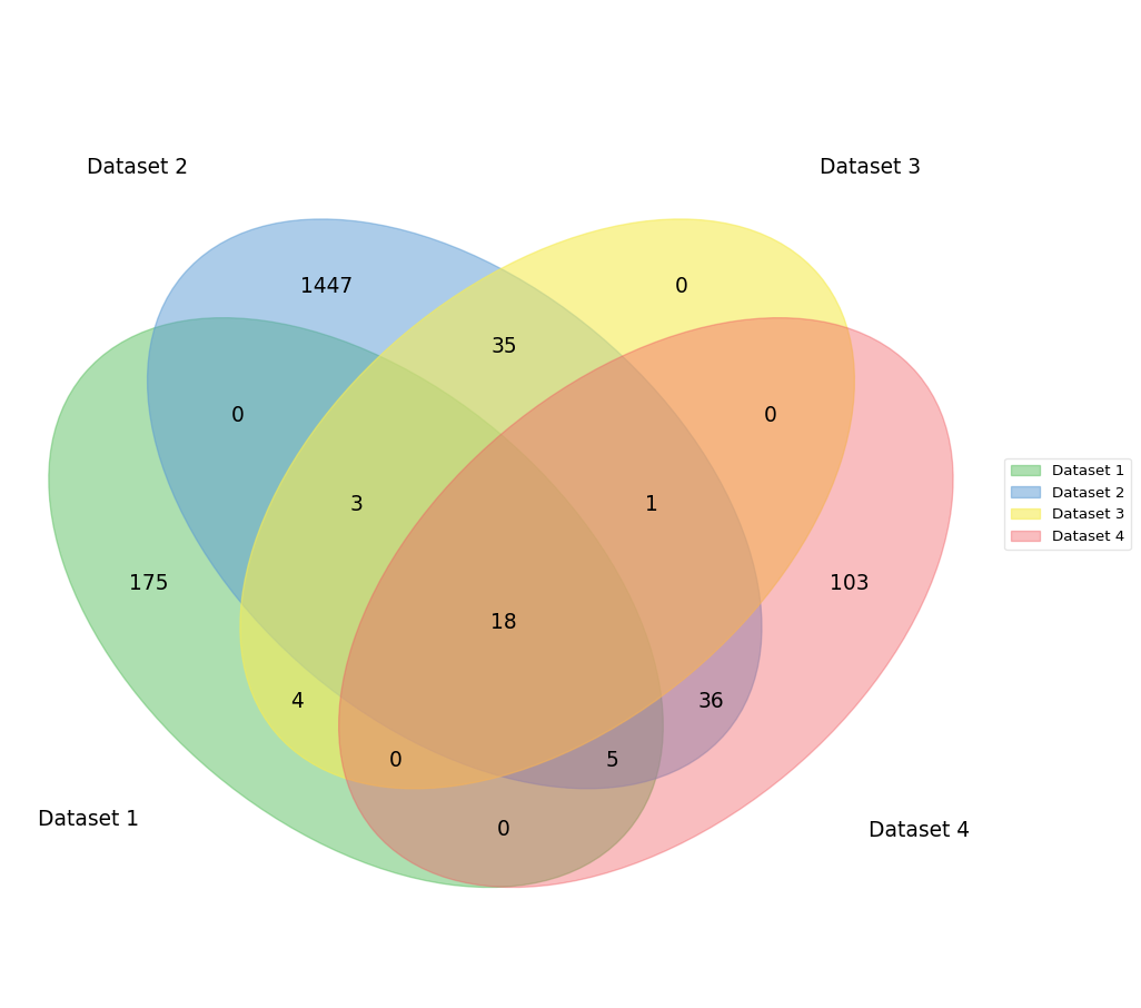
Figure 1: Overlap of attributes across datasets.

4 Related Work

Two model families – tree-based models and neural networks – are widely used for tabular analysis. Practitioners use tree-based models such as XGBoost for tabular data in many domains, specifically in data mining competitions [16]. Several studies showed that tree-based models outperformed neural networks for small to medium row sizes (less than 10K), while neural networks were superior for large-scale data [8, 25]. An advantage of neural networks is their adaptability to incorporate domain knowledge to design a network architecture suitable to the target dataset. Transformers [32] are an architecture that has been recently claimed to be promising for tabular modeling [1, 4, 7, 12, 13, 16, 26]. However, we employ the VAE architecture because it can handle uncertainty in the output.

5 Experiments

In this section, we evaluate the accuracy of the prediction model and the effectiveness of the model for enabling novel healthcare applications. Unless otherwise stated, we down-sample or up-sample the datasets for training depending on their sample sizes, as shown in Table 2. In particular, we reduced the sample size of Dataset 1 from 1.2 million to 100,000 because we observed that the prediction performance saturated around this sample size. We split the dataset into the train, validation, and test splits.

We first evaluate the prediction performance of the model in terms of error, its capability to capture pairwise correlation and the performance under the out-of-distribution (OOD) setting. Then, we conduct ablation studies to validate the effectiveness of masked modeling, mask augmentation, and $\beta$-annealing.

5.1 Evaluation Metrics

Here, we describe how to compute errors for each variable type. To calculate errors, we are given predictions and the ground truths of test entries for a column of interest: $Y^{\mathrm{pred}}=(y^{\mathrm{pred}}_{i})_{i=1}^{n_{\mathrm{test}}}$ and $Y^{\mathrm{test}}=(y^{\mathrm{test}}_{i})_{i=1}^{n_{\mathrm{test}}}$, respectively.

For categorical variables, we used average accuracy:

$$\mathrm{categorical\text{\_}error}(Y^{\mathrm{pred}},Y^{\mathrm{test}})=\frac{1}{n_{\mathrm{test}}}\sum_{i=1}^{n_{\mathrm{test}}}\llbracket y^{\mathrm{pred}}_{i}\not=y^{\mathrm{test}}_{i}\rrbracket,$$

where $\llbracket\cdot\rrbracket$ is the Iverson bracket that takes a logic expression as an argument and gives $1$ if the expression is true and $0$ otherwise.

For ordinal variables, we used mean absolute error normalized by the dimension of the label space:

$$\mathrm{ordinal\text{\_}error}(Y^{\mathrm{pred}},Y^{\mathrm{test}})=\frac{1}{n_{\mathrm{test}}}\sum_{i=1}^{n_{\mathrm{test}}}\frac{|y^{\mathrm{pred}}_{i}-y^{\mathrm{test}}_{i}|}{c},$$

where $c$ denotes the cardinality of the ordinal label space (ref. Eq. (2)).

For count, positive, and real variables, we used the root mean squared error normalized by the difference between the maximum and minimum of the ground truths:

$$\mathrm{continuous\text{\_}error}(Y^{\mathrm{pred}},Y^{\mathrm{test}})=\frac{\sqrt{\frac{1}{n_{\mathrm{test}}}\sum_{i=1}^{n_{\mathrm{test}}}(y^{\mathrm{pred}}_{i}-y^{\mathrm{test}}_{i})^{2}}}{\max(Y^{\mathrm{test}})-\min(Y^{\mathrm{test}})}.$$

5.2 Hyperparameters

Model architecture: We used one hidden layer with 320 hidden nodes. Dimensions of HIVAE for $s$, $z$, and $y$, which are $d_{\mathrm{s}}$, $d_{\mathrm{z}}$, and $d_{\mathrm{y}}$, were set to 70, 98, and $p$ (the number of attributes), respectively.

$\beta$-annealing: We used $\beta$-annealing that increases $\beta$ as the training progresses, where we initialized $\beta_{s}$ and $\beta_{z}$ as zero and linearly increased it to 0.30 and 0.04 at epoch 100, respectively. The values of $\beta_{s}$ and $\beta_{z}$ remained unchanged after epoch 100 until the training finished.

Mask augmentation: For each epoch, we randomly masked out the input features for 80% of the training data. Therefore, the missing pattern for each epoch is different so that the model can learn from different missing patterns.

Optimization: we used Adam with weight, where the learning rate was set to $9\times 10^{-4}$ with weight decay parameter as $2.5\times 10^{-4}$. The batch size was set to 1024, and the number of epochs was set to 200, where we employed early stopping with patience equal to 50. The validation objective is the average error of all columns and datasets by calculating the average error of all columns for each dataset and then calculating the average error among four datasets.

5.3 Prediction Performances

Here, we validate the effectiveness of using HIVAE as a model choice by comparing it with baselines, visualizing its pairwise correlation performance, and its capability to combat the out-of-distribution (OOD) setting.

Method	Categorical	Count	Ordinal	Positive	Real	Total
Mode Imputer	0.2824	0.1449	0.1358	0.1105	0.1675	0.1694
Mode-mean Imputer	0.2824	0.1210	0.1186	0.1082	0.1479	0.1513
Mode-median Imputer	0.2824	0.1193	0.1205	0.1102	0.1467	0.1507
Our Model	0.2375	0.1020	0.1140	0.0961	0.1205	0.1237

Table 3: Prediction Performance evaluated in terms of errors across different variable types.

5.3.1 Baseline Comparisons

Since the model needs to predict 1,827 attributes, as a validation of the model, we first verified whether a single model could make meaningful inferences.

For baselines, we compared the model with the mode imputer, which fills missing values with the mode in the training data set for each attribute. We note that the mode imputation can work for continuous attributes (real and positive variables) to some extent. This is because most numerical attributes have the smallest unit of measurement. Furthermore, we also compared the model with mode-mean imputer, where we used mean values for continuous attributes and rounded mean values for the count and ordinal attributes. We also used mode-median imputer, where we used median for continuous attributes and rounded median values for the count and ordinal attributes.

Table 3 shows the performance results. It can be observed that our model achieves better performance than the baselines. The output values of the baseline imputers only depend on the training dataset and do not depend on the inputs. Therefore, it can be concluded that our model successfully utilizes the information from the input records to make inferences.

5.3.2 Pairwise Correlations

We next examine whether our model learns the conditional distribution by comparing the pairwise correlation between attributes. We compute the correlation learned by the model between two real attributes $i$ and $j$ as follows: We input records whose entries are empty but the attribute $i$ whose values are equally spaced discretized values, for example, from 10 to 40 for Body Mass Index (BMI). We apply latent-sampling prediction to obtain $n$ pairs of mean and variance parameters ($n=100$ in our experiments).

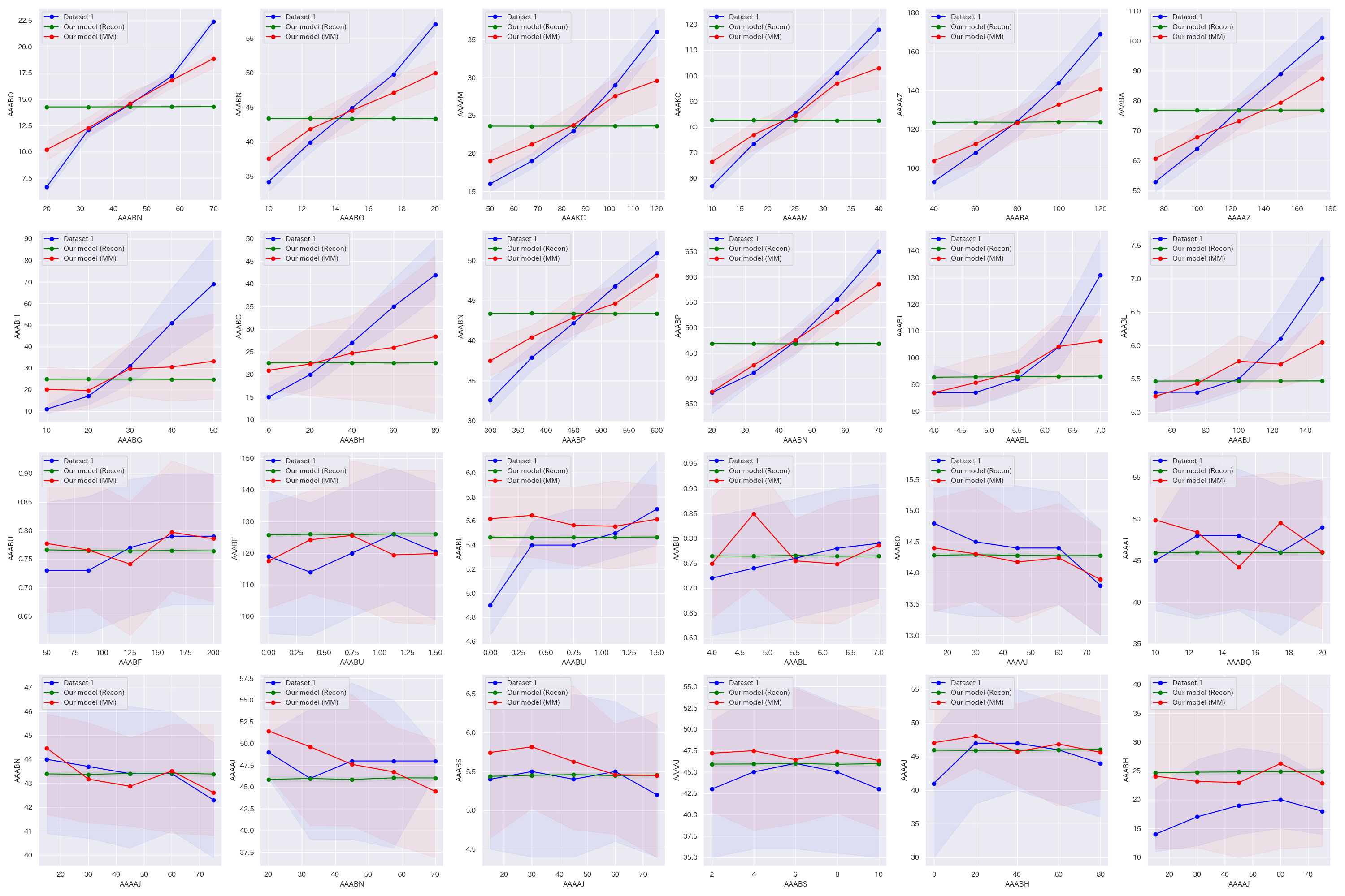
Figure 2: Pairwise correlation modeled by Dataset 1 (blue), our model with masked modeling (MM) loss (red), and reconstruction (Recon) loss (green). The upper two rows show the most correlated pairs and the lower two rows show the least correlated pairs. It can be observed that using our model with the masked modeling loss can capture pairwise correlation more effectively than using the reconstruction loss.

Figure 2 (left) compares the pairwise correlations inferred by the model (red) and empirical pairwise correlations (blue). We see that both correlations are close to each other for both highly correlated pairs and pairs with little correlations in most cases.

5.3.3 OOD Performance Evaluation

This section examines the effect of integrating tables with different characteristics for training. Since user queries can come from a distribution different from the training dataset, the performance in the OOD setting is highly useful for our application. In this experiment, we trained the model using Datasets 2–4 and evaluated the model on Dataset 1. As comparison methods, we use the models trained only on a single dataset (Dataset 2–4). Because each dataset has a different set of columns, we used only 18 attributes common to all datasets to train and test each model for a fair comparison. More specifically, we used only 14 real variables, two positive variables, one ordinal variable, and 1 categorical variable. In this case, combining datasets can have performance considerably close to training with the in-domain dataset (Dataset 1). Tables 7–7 show the result across the different train and test missing rates. The results illustrate that combining datasets improve the prediction accuracy in the OOD setting in most cases. Only the case where Dataset 3 is the OOD dataset in Table 7, where training the model using only Dataset 1 is preferable to combining Datasets 1, 2, and 4 to train the model.

Dataset	Missing Rate = 0.3	Missing Rate = 0.5	Missing Rate = 0.8
Dataset 2 + 3 + 4	0.0738 (0.0004)	0.0822 (0.0006)	0.0972 (0.0007)
Dataset 2	0.0811 (0.0007)	0.0868 (0.0005)	0.1047 (0.0005)
Dataset 3	0.0831 (0.0008)	0.0885 (0.0007)	0.0990 (0.0002)
Dataset 4	0.0945 (0.0013)	0.0967 (0.0006)	0.1110 (0.0005)
Dataset 1 (in-domain)	0.0725 (0.0007)	0.0833 (0.0009)	0.0958 (0.0006)

Table 4: Effect of table integration on performance for OOD evaluation. The metric is evaluated on the test dataset of Dataset 1 across the different train and test missing rates.

Dataset	Missing Rate = 0.3	Missing Rate = 0.5	Missing Rate = 0.8
Dataset 1 + 3 + 4	0.1353 (0.0011)	0.1478 (0.0022)	0.1823 (0.0014)
Dataset 1	0.1377 (0.0024)	0.1488 (0.0020)	0.1848 (0.0019)
Dataset 3	0.1467 (0.0012)	0.1607 (0.0008)	0.1954 (0.0004)
Dataset 4	0.1583 (0.0016)	0.1687 (0.0.008)	0.2070 (0.0015)
Dataset 2 (in-domain)	0.1343 (0.0038)	0.1413 (0.0019)	0.1788 (0.0009)

Table 5: Effect of table integration on performance for OOD evaluation. The metric is evaluated on the test dataset of Dataset 2 across the different train and test missing rates.

Dataset	Missing Rate = 0.3	Missing Rate = 0.5	Missing Rate = 0.8
Dataset 1 + 2 + 4	0.0971 (0.0007)	0.1042 (0.0006)	0.1207 (0.0006)
Dataset 1	0.0951 (0.0007)	0.1025 (0.0005)	0.1179 (0.0006)
Dataset 2	0.1077 (0.0011)	0.1144 (0.0008)	0.1353 (0.0012)
Dataset 4	0.1169 (0.0017)	0.1254 (0.0007)	0.1431 (0.0010)
Dataset 3 (in-domain)	0.0969 (0.0006)	0.1020 (0.0003)	0.1154 (0.0002)

Table 6: Effect of table integration on performance for OOD evaluation. The metric is evaluated on the test dataset of Dataset 3 across the different train and test missing rates.

Dataset	Missing Rate = 0.3	Missing Rate = 0.5	Missing Rate = 0.8
Dataset 1 + 2 + 3	0.1036 (0.0010)	0.1166 (0.0006)	0.1384 (0.0005)
Dataset 1	0.1047 (0.0009)	0.1174 (0.0015)	0.1383 (0.0006)
Dataset 2	0.1093 (0.0019)	0.1225 (0.0006)	0.1423 (0.0009)
Dataset 3	0.1263 (0.0005)	0.1338 (0.0009)	0.1498 (0.0002)
Dataset 4 (in-domain)	0.0939 (0.0009)	0.1026 (0.0004)	0.1245 (0.0007)

Table 7: Effect of table integration on performance for OOD evaluation. The metric is evaluated on the test dataset of Dataset 4 across the different train and test missing rates.

5.4 Ablation Studies

Here, we validate the usefulness of the techniques we used for training the model.

5.4.1 Masked Modeling Loss vs. Reconstruction Loss

In masked modeling, the model is trained to predict the masked entries. We can instead train the model to reconstruct the unmasked entries similar to the denoising autoencoder. Table 10 shows the performance comparisons between our model trained with and without masked modeling loss. It can be observed that using masked modeling can achieve better performance. Next, the pairwise correlation performance is investigated. Figure 2 shows the pairwise correlations inferred by the model learned by the reconstruction of unmasked entries (Recon). Unlike the model learned by masked modeling (MM), the $y$-axis values tend to remain unchanged even if we change the $x$-axis values for highly correlated pairs. This result suggests that the model learned by minimizing the reconstruction loss cannot effectively capture the pairwise correlation of the attributes. On the other hand, the model learned by masked modeling is observed to be effective for capturing the correlation of attributes.

5.4.2 Mask Augmentation

In this section, we examine the effect of mask augmentation. In the comparison method, we determine the mask pattern at the beginning of training and fix the pattern during training. Table 10 shows the difference in prediction accuracy with and without mask augmentation. The result shows that mask augmentation improves the accuracy of the imputation.

5.4.3 $\beta$-annealing

Next, we evaluate the effect of $\beta$-annealing. We trained the model using the loss function (3), except that we set $\beta^{(t)}_{\mathrm{s}}=\beta^{(t)}_{\mathrm{z}}=1$ for all $t$. Table 10 compares prediction accuracy with and without $\beta$-annealing. The results show that $\beta$-annealing improves the prediction accuracy.

Loss	Categorical	Count	Ordinal	Positive	Real	Total
MM	0.2151 (0.012)	0.0989 (0.001)	0.1139 (0.001)	0.0950 (0.001)	0.1210 (0.001)	0.1232 (0.001)
Recon	0.2546 (0.018)	0.1017 (0.003)	0.1157 (0.001)	0.1090 (0.001)	0.1348 (0.001)	0.1331 (0.001)

Table 8: Comparison between using Masked modeling (MM) loss and Reconstruction loss (Recon) for HIVAE.

Mask aug.	Categorical	Count	Ordinal	Positive	Real	Total
Used	0.2151 (0.012)	0.0989 (0.001)	0.1139 (0.001)	0.0950 (0.001)	0.1210 (0.001)	0.1232 (0.001)
Not used	0.2216 (0.011)	0.1080 (0.005)	0.1165 (0.002)	0.0987 (0.005)	0.1254 (0.005)	0.1269 (0.003)

Table 9: Effect of mask augmentation on performance.

$\beta$-annealing	Categorical	Count	Ordinal	Positive	Real	Total
Used	0.2151 (0.012)	0.0989 (0.001)	0.1139 (0.001)	0.0950 (0.001)	0.1210 (0.001)	0.1232 (0.001)
Not used	0.2266 (0.023)	0.1015 (0.001)	0.1193 (0.001)	0.1000 (0.001)	0.1253 (0.001)	0.1276 (0.001)

Table 10: Effect of $\beta$-annealing on the performance.

6 System

6.1 Overview

VHGM is provided as an integral part of a lifecare application platform. Figure 3 shows the overview of the platform. Any application program on the platform calls VHGM via APIs. The platform also provides other lifecare-related services, such as measurement and intervention services, so that innovative lifecare applications can be built by combining these services. With its broad coverage of lifecare attributes, VHGM is expected to play a vital role in interrelating a diverse set of measurements and intervention services. For example, an application would call a measurement service to get blood test results of the end user, estimate the probabilities of various diseases of people who have similar blood test results, and suggest the user take supplements provided by an intervention service.

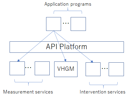
Figure 3: Platform Overview.

6.2 APIs

VHDM provides two types of prediction as APIs: latent-deterministic prediction and latent-sampling prediction. The latent-deterministic prediction API takes a record that possibly has missing values and returns the distribution parameters $\gamma=(\gamma_{1},\ldots,\gamma_{p})$. The inference is deterministic in the sense that it does not use both the predictive-distribution sampling and the latent-variable sampling (Section 3.3). This API also provides the point estimate of each attribute by the mode value of the distribution with the parameter $\gamma$. On the other hand, the latent-sampling prediction API takes the sampling size $N$ along with an input record. It computes the set of distribution parameters $\gamma^{(1)},\ldots,\gamma^{(N)}$ by applying the latent-variable sampling $N$ times. We can evaluate the uncertainty of the posterior distribution by the variability of the $\gamma$ parameters. We can optionally compute the point estimate of missing values for both APIs by applying the predictive-distribution sampling using the returned parameters.

6.3 Dataset Management and Model Deployment

One of the challenges of VHDM is the heterogeneity of datasets for training. Datasets have different sets of attributes, and some attributes, such as basic demographic information, are semantically the same but differ in notations and scales among datasets. In addition, we sometimes need to update datasets, for example, by adding and deleting columns and fixing bugs in metadata and data themselves.

We adopt dataset schema to manage multiple datasets and their updates systematically. The dataset schema is a list of metadata of available attributes such as ID, name, variable type, and possible values (for categorical values). We regularly update the schema to define the set of attributes the model employs. Accordingly, datasets are updated and processed to comply with the schema. That is, the attribute set of each dataset is a subset of the schema. Following updating the dataset schema and datasets, we re-train and deploy the model to the system.

7 Applications

7.1 Virtual Measurement

The system’s most straightforward usage is to estimate an individual’s unknown attributes from known ones. This is useful when some attributes are hard to measure while others are not. For example, we can estimate, with some uncertainty, the value of an attribute that is expensive to measure from relatively inexpensive ones, such as systolic blood pressure and demographic attributes (e.g., age and sex).

7.2 Relative Positioning in a Group

For any group of people characterized by a set of attribute values (e.g., males in their 50s with smoking and drinking habits), VHGM can give a probability distribution of this group for any other attribute. This is useful when one needs to understand their relative positioning in that particular group. For example, we may find a person with low blood glucose level considering their demography and lifestyle.

7.3 Hypothetical Scenarios

By changing some attributes to hypothetical values, one can compare different scenarios. For example, a person in his thirties would ask suppose there would be a population of people with the same health information as me except that their age is 50, how would their glucose values differ from mine? We can obtain the answer to this question by entering our health information, changing only the person’s age from thirty to fifty, and seeing how the estimated glucose level differs from their actual value (or its estimate).

7.4 Exploration of Best Scenario

By exploring multiple hypothetical scenarios, we can use this system to search for a population whose specific attributes have desired values. For example, suppose we want to know what groups would have the lowest blood pressure with the same healthcare information as mine? To answer this question, we first define a set of groups and then, using VHGM, search for the group with the lowest blood pressure estimate. The search could be done by a simple grid search algorithm or a more sophisticated black-box optimization tool.

7.5 Demo Application

We developed a web application to provide inferences based on given values using the VHGM APIs. Figure 4 shows a browser window of the application. Biological gender, age, height, weight, and BMI were given as input data (Figure 4, top left), and all attributes except for the given input were estimated (Figure 4, top right). This demonstration also provides hypothetical scenarios. For example, Figure 4 (bottom left) shows an example output of the scenario: if my age were 60 years old, my weight were 80 kg, and my BMI were 27.7. In this case, visceral fat area, LDL-cholesterol, and fasting blood glucose are highlighted in red, indicating higher than the original ones. In addition, one can compare two lifestyle scenarios. In Figure 4 (bottom right), we compare two scenarios of differing walking habits, whether one has walking or an equivalent amount of physical activity more than one hour a day in their daily activity. This application allows us to explore which attributes could change if a hypothetical scenario occurs.

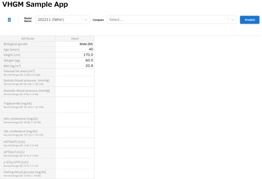
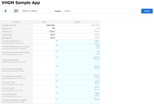
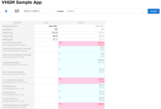
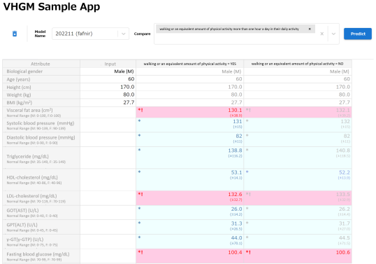
Figure 4: Top: Demo Application. Bottom left: What-if scenario. Bottom right: Comparison between two scenarios. Note that only 17 attributes are displayed due to space limitations.

8 Challenges and Limitations

8.1 Masking Strategy

In this study, we employed a relatively simple masking strategy: we fixed a probability $\alpha$ and chose the cells to be masked uniformly randomly with the ratio of $\alpha$. It is room for discussion about whether this masking strategy is optimal. In fact, in language models, the performance of masked modeling can be improved by combining several masking strategies [30]. Better masking strategies for masked modeling on tabular data are future work.

8.2 Causality

The model learns the joint distribution of attributes and does not use the information on their causality. Therefore, when we modify some of the input attributes, we should not interpret that the input change causes the output change. It should be noted that VHGM only shows the statistical interactions among attributes and does not represent any causal relations. Thus, the what-if use cases in Section 7.4 should not be interpreted as causal inferences. In case causal interpretations are necessary, the output of VHGM must be combined with a priori knowledge about causal relations.

8.3 Time-series Analysis

The current training data set has no time-series information on the same subject. Therefore, performing a time series analysis with this model is inadequate. Although one application in Section 7.3 compares the distributions of attributes between groups of different ages, it does not mean that they predict the future values; Instead, they are the estimates under the hypothetical assumption on their ages. Therefore, this analysis does not imply the future values of the person.

9 Conclusion

In this paper, we proposed Virtual Human Generative Model (VHGM), a statistical model for the joint distribution of observable healthcare data, lifestyles, and personalities of people. The core of VHGM is a Heterogeneous-Imcomplete Variational Autoencoder (HIVAE), a deep generative model for tabular data that estimates unknown attributes from known attributes of healthcare with the uncertainty of the estimations. We employed several techniques in training, such as masked modeling and integrating tabular datasets of different characteristics. These techniques enabled efficient modeling of simultaneous probability distributions conditioned on inputs for over 1,800 healthcare attributes. The inference service using VHGM is provided as APIs on a platform on which third-party application vendors can develop healthcare applications. We presented the use cases of the VHGM API, virtual measurement of healthcare attributes, and comparing and recommending hypothetical lifestyles. We believe the versatility of VHDM leads to a wide range of healthcare applications, thereby contributing to the social good of enhancing people’s quality of life.

References

- [1] S. O. Arik and T. Pfister. TabNet: Attentive interpretable tabular learning. Proceedings of the AAAI Conference on Artificial Intelligence, 35(8):6679–6687, May 2021.
- [2] S. R. Bowman, L. Vilnis, O. Vinyals, A. Dai, R. Jozefowicz, and S. Bengio. Generating sentences from a continuous space. In Proceedings of the 20th SIGNLL Conference on Computational Natural Language Learning, pages 10–21, Berlin, Germany, Aug. 2016. Association for Computational Linguistics.
- [3] A. Chikama, T. Yamaguchi, T. Watanabe, K. Mori, Y. Katsuragi, I. Tokimitsu, O. Kajimoto, and M. Kitakaze. Effects of chlorogenic acids in hydroxyhydroquinone-reduced coffee on blood pressure and vascular endothelial function in humans. Prog Med, 26:1723–1736, 2006.
- [4] X. Deng, H. Sun, A. Lees, Y. Wu, and C. Yu. Turl: Table understanding through representation learning. arXiv preprint arXiv:2006.14806, 2020.
- [5] J. Devlin, M.-W. Chang, K. Lee, and K. Toutanova. BERT: Pre-training of deep bidirectional transformers for language understanding. In Proceedings of the 2019 Conference of the North American Chapter of the Association for Computational Linguistics: Human Language Technologies, Volume 1 (Long and Short Papers), pages 4171–4186, Minneapolis, Minnesota, June 2019. Association for Computational Linguistics.
- [6] H. Fu, C. Li, X. Liu, J. Gao, A. Celikyilmaz, and L. Carin. Cyclical annealing schedule: A simple approach to mitigating KL vanishing. In Proceedings of the 2019 Conference of the North American Chapter of the Association for Computational Linguistics: Human Language Technologies, Volume 1 (Long and Short Papers), pages 240–250, Minneapolis, Minnesota, June 2019. Association for Computational Linguistics.
- [7] Y. Gorishniy, I. Rubachev, V. Khrulkov, and A. Babenko. Revisiting deep learning models for tabular data. arXiv preprint arXiv:2106.11959, 2021.
- [8] L. Grinsztajn, E. Oyallon, and G. Varoquaux. Why do tree-based models still outperform deep learning on tabular data? arXiv preprint arXiv:2207.08815, 2022.
- [9] K. He, X. Chen, S. Xie, Y. Li, P. Dollár, and R. Girshick. Masked autoencoders are scalable vision learners. In Proceedings of the IEEE/CVF Conference on Computer Vision and Pattern Recognition (CVPR), pages 16000–16009, June 2022.
- [10] M. Hibi, S. Katada, A. Kawakami, K. Bito, M. Ohtsuka, K. Sugitani, A. Muliandi, N. Yamanaka, T. Hasumura, Y. Ando, T. Fushimi, T. Fujimatsu, T. Akatsu, S. Kawano, R. Kimura, S. Tsuchiya, Y. Yamamoto, M. Haneoka, K. Kushida, T. Hideshima, E. Shimizu, J. Suzuki, A. Kirino, H. Tsujimura, S. Nakamura, T. Sakamoto, Y. Tazoe, M. Yabuki, S. Nagase, T. Hirano, R. Fukuda, Y. Yamashiro, Y. Nagashima, N. Ojima, M. Sudo, N. Oya, Y. Minegishi, K. Misawa, N. Charoenphakdee, Z. Gao, K. Hayashi, K. Oono, Y. Sugawara, S. Yamaguchi, T. Ono, and H. Maruyama. Assessment of multidimensional health care parameters among adults in japan for developing a virtual human generative model: Protocol for a cross-sectional study. JMIR Res Protoc, 12:e47024, Jun 2023.
- [11] I. Higgins, L. Matthey, A. Pal, C. Burgess, X. Glorot, M. Botvinick, S. Mohamed, and A. Lerchner. beta-VAE: Learning basic visual concepts with a constrained variational framework. In International Conference on Learning Representations, 2017.
- [12] X. Huang, A. Khetan, M. Cvitkovic, and Z. Karnin. Tabtransformer: Tabular data modeling using contextual embeddings. arXiv preprint arXiv:2012.06678, 2020.
- [13] H. Iida, D. Thai, V. Manjunatha, and M. Iyyer. Tabbie: Pretrained representations of tabular data. arXiv preprint arXiv:2105.02584, 2021.
- [14] E. Jang, S. Gu, and B. Poole. Categorical reparameterization with gumbel-softmax. In International Conference on Learning Representations, 2017.
- [15] D. P. Kingma and M. Welling. Auto-Encoding Variational Bayes. In 2nd International Conference on Learning Representations, ICLR 2014, Banff, AB, Canada, April 14-16, 2014, Conference Track Proceedings, 2014.
- [16] J. Kossen, N. Band, C. Lyle, A. N. Gomez, T. Rainforth, and Y. Gal. Self-attention between datapoints: Going beyond individual input-output pairs in deep learning. arXiv preprint arXiv:2106.02584, 2021.
- [17] K. Kozuma, A. Chikama, E. Hoshino, K. Kataoka, K. Mori, T. Hase, Y. Katsuragi, I. Tokimitsu, and H. Nakamura. Effect of intake of a beverage containing 540 mg catechins on the body composition of obese women and men. Prog Med, 25(7):1945–57, 2005.
- [18] Y. Matsui, K. Kinoshita, N. Osaki, T. Wakisaka, M. Hibi, Y. Katsuragi, T. Yamaguchi, and I. Fukuhara. Effects of tea catechin-rich beverage on abdominal fat area and body weight in obese japanese individuals - a randomized, double-blind, placebo-controlled, parallel-group study -. Jpn Pharmacol Ther, 46(8):1383–1395, 2018.
- [19] Y. Matsui, M. Takeshita, M. Hibi, I. Fukuhara, and N. Osaki. Efficacy and safety of powdered beverage containing green tea catechins on body fat in obese adults - a randomized, placebo controlled, double-blind parallel study. Jpn Pharmacol Ther, 44(7):1013–1023, 2016.
- [20] T. Nagao, T. Hase, and I. Tokimitsu. A green tea extract high in catechins reduces body fat and cardiovascular risks in humans. Obesity, 15(6):1473–1483, 2007.
- [21] T. Nagao, R. Ochiai, Y. Katsuragi, Y. Hayakawa, K. Kataoka, M. Komikado, I. Tokimitsu, and T. Tsuchida. Hydroxyhydroquinone-reduced milk coffee decreases blood pressure in individuals with mild hypertension and high-normal blood pressure. Prog Med, 27:2649–2664, 2007.
- [22] T. Nagao, R. Ochiai, T. Watanabe, K. Kataoka, M. Komikado, I. Tokimitsu, and T. Tsuchida. Visceral fat–reducing effect of continuous coffee beverage consumption in obese subjects. Jpn Pharmacol Ther, 37(4):333–344, 2009.
- [23] A. Nazábal, P. M. Olmos, Z. Ghahramani, and I. Valera. Handling incomplete heterogeneous data using vaes. Pattern Recognition, 107:107501, 2020.
- [24] H. Shao, S. Yao, D. Sun, A. Zhang, S. Liu, D. Liu, J. Wang, and T. Abdelzaher. ControlVAE: Controllable variational autoencoder. In H. D. III and A. Singh, editors, Proceedings of the 37th International Conference on Machine Learning, volume 119 of Proceedings of Machine Learning Research, pages 8655–8664. PMLR, 13–18 Jul 2020.
- [25] R. Shwartz-Ziv and A. Armon. Tabular data: Deep learning is not all you need. arXiv preprint arXiv:2106.03253, 2021.
- [26] G. Somepalli, M. Goldblum, A. Schwarzschild, C. B. Bruss, and T. Goldstein. Saint: Improved neural networks for tabular data via row attention and contrastive pre-training. arXiv preprint arXiv:2106.01342, 2021.
- [27] H. Takase, T. Nagao, K. Otsuka, K. Kozuma, S. Meguro, M. Komikado, and I. Tokimitsu. Effects of long-term ingestion of tea catechins on visceral fat accumulation and metabolic syndrome – pooling analysis of 7 randomized controlled trials. Jpn Pharmacol Ther, 36(6):509–514, 2008.
- [28] H. Takase, N. Sakane, T. Morimoto, T. Uchida, K. Mori, M. Katashima, and Y. Katsuragi. Development of a dietary factor assessment tool for evaluating associations between visceral fat accumulation and major nutrients in japanese adults. Journal of Obesity, 2019:9497861, Feb 2019.
- [29] M. Takeshita, S. Takashima, U. Harada, E. Shibata, N. Hosoya, H. Takase, K. Otsuka, S. Meguro, M. Komikado, and I. Tokimitsu. Effects of long-term consumption of tea catechins-enriched beverage with no caffeine on body composition in humans. Jpn Pharmacol Ther, 36:767–776, 2008.
- [30] Y. Tay, M. Dehghani, V. Q. Tran, X. Garcia, D. Bahri, T. Schuster, H. S. Zheng, N. Houlsby, and D. Metzler. Unifying language learning paradigms. arXiv preprint arXiv:2205.05131, 2022.
- [31] T. Tsuchida, H. Itakura, and H. Nakamura. Reduction of body fat in humans by long-term ingestion of catechins. Prog Med, 22:2189–2203, 2002.
- [32] A. Vaswani, N. Shazeer, N. Parmar, J. Uszkoreit, L. Jones, A. N. Gomez, L. Kaiser, and I. Polosukhin. Attention is all you need. arXiv preprint arXiv:1706.03762, 2017.
- [33] T. Watanabe, S. Kobayashi, T. Yamaguchi, M. Hibi, I. Fukuhara, and N. Osaki. Coffee abundant in chlorogenic acids reduces abdominal fat in overweight adults: A randomized, double-blind, controlled trial. Nutrients, 11(7):1617, 2019.
- [34] T. Yamaguchi, A. Chikama, M. Inaba, R. Ochiai, Y. Katsuragi, I. Tokimitsu, T. Tsuchida, and I. Saito. Antihypertensive effects of hydroxyhydroquinone-reduced coffee on high-normal blood pressure. Prog Med, 27:683–694, 2007.
- [35] S. Zhao, J. Song, and S. Ermon. A lagrangian perspective on latent variable generative models. pages 1031–1041, 6–10 Jun 2018.