Weierstrass elliptic functions for the pendulum

Abstract.

The mathematical pendulum is traditionally solved using a Jacobi elliptic functions. We solve it here using the Weierstrass elliptic function. Every initial condition of the pendulum produces an elliptic curve and a point which by the dynamics of the pendulum is translated linearly on the torus.

2. A polynomial differential equation

2.1.

The mathematical pendulum is the second order nonlinear differential equation

$$\theta^{\prime\prime}=4c\sin(\theta)\;.$$

The constant $c$ is a real parameter which in a physical setup would be $c=-g/(4l)$, where $g$ is the gravitational strength and $l$ is the length of the pendulum rod. The pendulum has the conserved energy $E=\theta^{\prime 2}/2+4c\cos(\theta)$ and is so a Hamiltonian system $x^{\prime}=H_{y},y^{\prime}=-H_{x}$ for the Hamiltonian

$$H(x,y)=\frac{y^{2}}{2}+4c\cos(x)$$

on the cylinder $\mathbb{T}\times\mathbb{R}$. Traditionally, the solution is obtained by solving the energy equation for $\theta^{\prime}$ then separate the variables $t,\theta$ and inverting a Jacobi elliptic integral. We proceed differently using Weierstrass elliptic curves.

2.2.

We start by setting $u=e^{i\theta}\in\mathbb{C}$. This produces a polynomial differential equation of second order, where $u^{\prime\prime}=\frac{d^{2}}{dt^{2}}u$ is the second derivative for a real or complex time $t$.

Lemma 1 (Polynomial Pendulum Equation).

$u^{\prime\prime}=6cu^{2}-2Eu+2c$.

Proof.

From $u^{\prime}=iu\theta^{\prime}$ and using $\theta^{\prime 2}u=2Eu-4c(u^{2}+1)$ and $i\theta^{\prime\prime}u=i4cu\sin(\theta)=2c(u^{2}-1)$, we have

$$u^{\prime\prime} = -u\theta^{\prime 2}+iu\theta^{\prime\prime}$$

$$= -2Eu+4c(u^{2}+1)+2c(u^{2}-1)$$

$$= 6cu^{2}-2Eu+2c\;.$$

∎

2.3.

For $u=w+E/(6c)$ we an depress the quadratic polynomial to the right and get $w^{\prime\prime}=6cw^{2}+a$, where $a=2c-E^{2}/(6c)$. With the new variable $p=w/c^{1/3}$ and the new time $z=c^{1/3}t$ and $g_{2}=-2a/c^{2/3}$, we arrive at the differential equation

$$p^{\prime\prime}=6p^{2}-g_{2}/2\;.$$

This differential equation is solved by $p(z)=\wp(z+g_{1},g_{2},g_{3})$, where the initial conditions $(\theta(0),\theta^{\prime}(0))$ defines the elliptic curve

$$\wp^{\prime 2}=4\wp^{3}-g_{2}\wp-g_{3}$$

and a point $g_{1}$ on it. As we have $g_{2}$ given from the energy, the constant $g_{3}$ is obtained from the initial conditions $w_{3}=-\wp^{\prime 2}(0)+4\wp^{3}(0)-g_{2}\wp(0)$ and $g_{1}$ is fixed from the initial conditions.

2.4. The Weierstrass elliptic function

2.5.

Any two complex numbers $\omega_{1},\omega_{2}$ which define linearly independent real vectors in $\mathbb{R}^{2}$ define a lattice $\Lambda=\{n\omega_{1}+m\omega_{2}\;|\;n,m\in\mathbb{Z}\}$, the 2-torus $\mathbb{T}^{2}=\mathbb{R}^{2}/\Lambda$ and the Weierstrass elliptic function summing over all non-zero lattice points $\dot{\Lambda}$:

$$\wp(z)=\frac{1}{z^{2}}+\sum_{\lambda\in\dot{\Lambda}}\frac{1}{(z-\lambda)^{2}}-\frac{1}{\lambda^{2}}\;.$$

2.6.

The $\wp$ satisfies the differential equation

$$\wp^{\prime}(z)^{2}=4\wp(z)^{3}-g_{2}\wp(z)-g_{3}\;,$$

where $g_{2},g_{3}$ are determined by the lattice $\Lambda$ so that $(\wp(z),\wp^{\prime}(z))$ are on the elliptic curve

$$y^{2}=4x^{3}-g_{2}x-g_{3}\;.$$

One just needs to realize that $\wp^{\prime}(z)^{2}-4\wp(z)^{3}+g_{2}\wp(z)$ is analytic and so constant [1]. The elliptic curve over $\mathbb{C}$ is a 2-torus if the discriminant $\Delta=g_{2}^{3}-27g_{3}^{2}$ is non-zero. Slightly less well known is that $\wp$ satisfies a second order quadratic differential equation:

Lemma 2.

For arbitrary complex $g_{1},g_{2},g_{3}$, the function $p(z)=\wp(z+g_{1},g_{2},g_{3})$ is the general solution of the differential equation $p^{\prime\prime}=6p^{2}-g_{2}/2$.

Proof.

Differentiate the definition of $\wp$ to get $\wp^{\prime}=-2\sum_{\lambda\in\Lambda}\frac{1}{(z-\lambda)^{3}}$ and $\wp^{\prime\prime}=6\sum_{\lambda\in\Lambda}\frac{1}{(z-\lambda)^{4}}$. The function $6\wp^{2}-\wp^{\prime\prime}$ has lost its singularity at $0$ so that $6(\sum_{\lambda\neq 0\in\Lambda}(\frac{1}{(z-\lambda)^{2}})^{2}-\frac{1}{\lambda^{2}})-6\sum_{\lambda\neq 0\in\Lambda}\frac{1}{(z-\lambda)^{4}}$ is analytic on the torus and therefore must be constant by Liouville’s theorem. Evaluated at $z=0$, to see the constant is $g_{2}/2$. ∎

2.7.

As for the literature, [11] page 61 derives it by differentiating $\wp^{\prime}(z)^{2}=4\wp(z)-g_{2}\wp(z)-g_{3}$ with respect to $z$ and dividing by $\wp^{\prime}(z)$. It also appears as Problem 2.4.1 in [10] and is subject of Corollary 7.1 of [2].

2.8.

The upshot is that the solution of the mathematical pendulum equation can be explicitly written down as $\theta(t)=\arg(a+b\wp(qt+g_{1},g_{2},g_{3}))$, where $a,b,q$ are constants depending on $c$, and $g_{1},g_{2},g_{3}$ depend on $\theta_{0},\theta^{\prime}(0)$ and $c$. The pendulum trajectory is a closed path on the elliptic curve provided $\Delta\neq 0$. This is an elegant alternative to the solution given as amplitudes of Jacobi elliptic functions [2], which computer algebra system get to when asking for a solution (like with $DSolve[x^{\prime\prime}[t]==4cSin[x[t]],x[t],t]$ in Mathematica).

3. Pendulum dynamics in the unitary group

3.1.

The pendulum equation is related to the Lie group $U(1)$. This can be generalized to the unitary $U(n)=\{A\in M(n,\mathbb{C}),A^{*}A=1_{n}\}$ if the initial conditions commute Every such group element $A$ can be written as $A=e^{i\theta}$ where $a=i\theta$ are skew Hermitian matrices $a^{*}=-a$. The same integrates also matrix differential equations $\theta^{\prime\prime}=4c\sin(\theta)$, where $\theta,\theta^{\prime}$ are commuting Hermitian matrices.

3.2.

The computation we just did in the Lie algebra $g=\mathbb{R}$ of the compact Lie group $G=U(1)$ can be done on any Lie algebra $g$ of the unitary group $G=U(n)$ as the elements of the Lie algebra are given by Hermitian matrices $x$ so that $\sin$ preserves the Lie algebra. We get so integrable systems on a subset of $G=U(n)$. Write an element in the Lie algebra as $a=i\theta$ and an element in the Lie group as $u=e^{i\theta}$, then separate $e^{i\theta}=\cos(\theta)+i\sin(\theta)$, each $\theta$ is linear space of matrices, the exponential can be understood in a linear algebra sense so that $e^{i\theta}$ is a matrix, representing the group element in $G$. Rules like $\sin^{\prime}(\theta)=\cos(\theta)$ are satisfied by functional calculus because Hermitian matrices are normal.

3.3.

The differential equation $\theta^{\prime\prime}=4c\sin(\theta)$ in the Lie algebra produces curves $\theta(t)$ in the vector space of Hermitian matrices and the energy $E=\theta^{\prime 2}/2+4c\cos(\theta)$ is conserved if the initial $\theta,\theta^{\prime}$ commute. The differential equation $\theta^{\prime\prime}=4c\sin(\theta)$ has invariant measure of the Hamiltonian flow is located either on an equilibrium point or some $k$-dimensional real torus with $k\leq n$.

Proof.

One can diagonalize the $\theta$ reducing the system to $n$ independent penduli or proceed as before: define $u=e^{i\theta}$ $w$ with $u=w+E/(6c)$ and $p=w/c^{1/3}$ and the new time $z=t/c^{1/3}$ so that $p^{\prime\prime}=6p^{2}-g_{2}/2$, where $g_{2}$ is identified with $g_{2}I$ in the matrix algebra $G$. This means that $p(z)\in M(n,\mathbb{C})$ satisfies the Weierstrass differential equation. To every matrix entry $p_{ij}(z)\in\mathbb{C}$ is now associated an elliptic curve. If the initial condition $\theta$ and velocity $\theta^{\prime}$ are such that for all $i,j$, the elliptic curve describing $p_{ij}(z)$ is non-degenerate, then the solution curve $p_{ij}(t)$ moves on a straight line in a $d$-dimensional torus. Once we have determined $p(t)$, we can get $u(t)=c^{1/3}p(t)+E/(6c)$ and get $\theta(t)={\rm arg}(u(t))$, where the arg function takes an element in the Lie group $U(n)$ and associates to it $\theta(t)$ such that $e^{i\theta(t)}=u(t)$. ∎

3.4.

For almost all initial condition, the solution is dense and Diophantine and survives by KAM theory small perturbations of the Hamiltonian. Also, by general principles, arbitrary small perturbations of the Hamiltonian can now achieve that there are weakly mixing invariant tori [8].

Corollary 1.

There are arbitrary small perturbations of the pendulum Hamiltonian in the unitary group $U(n)$ for $n\geq 2$ such that the system has weakly mixing invariant tori.

3.5.

If $\theta(0),\theta^{\prime}(0)$ are simultaneously diagonalizable, we just have a copy of $1$-dimensional systems. What is special about the above differential equation is that $(p(0),p^{\prime}(0))\in TU(n)$ determines for every matrix entry an elliptic curve solving also the matrix equation. The Weierstrass integration works if we assume that the initial position and velocity commute and so are simultaneously diagonalizable.

4. Remarks

4.1.

Any Hamiltonian system in a 2-dimensional phase space $M$ is integrable because the energy function $H$ foliates $M$ into level curves which are 1-manifolds at non-critical values of $H$. Going beyond Hamiltonian systems, topology starts to matter for the existence of non-integrable cases: by Poincaré-Bendixon, every differential equation on the plane (or the compactified sphere) is integrable in the sense that every flow-invariant measure is supported on the fixed point set or on a finite collection of periodic orbits. There are vector fields on $\mathbb{T}^{2}$ already with weakly mixing invariant measures [3, 5]. The pendulum is special because integrability carries over to the Sin-Gordon partial differential equations $\theta_{tt}-\theta_{xx}=4c\sin(\theta)$. One also has integrability for discrete Sin-Gordon equations $\theta_{tt}-L\theta=4c\sin(\theta)$, where $\theta$ is a function on the vertices of a graph and $L$ the Kirchhoff Laplacian of the graph. The pendulum can also be seen as a 2-particle Toda system and so a Lax Pair description [7]. It seems that the Today system is the right higher dimensional non-linear generalization of the pendulum.

4.2.

A long-standing open problem in Hamiltonian dynamics is the question of Kolmogorov, whether there are examples of Hamiltonian systems with mixing invariant tori. This reportedly had been a motivation for Kolmogorov to develop KAM theory [9]. We had remarked in 1999 [8] that it is possible to always get from an invariant KAM torus a weakly mixing invariant $d$-torus with $d\geq 2$ using arbitrary small perturbations. This works even in infinite dimensions if an invariant finite dimensional torus exists on which one has a quasi-periodic motion. The idea was that on two or larger dimensional tori, the linear ergodic flow can be perturbed so that ergodicity and pure point spectrum upgrades to singular continuity and so leads to weak mixing. Already the flow $\theta^{\prime\prime}=4c\sin(\theta)$ on the Lie algebra of $U(2)$ produces for almost all initial conditions $(\theta,\theta^{\prime})$ an orbit that is dense on a $2$-dimensional real torus in $U(2)$. A small perturbation of the Hamiltonian can now produce solution curves $z(t)=\exp(i\theta(t))\in U(2)$ which show a weak type of chaos.

4.3.

Let us end this note with a remark on our motivation. A core tool in smooth ergodic theory is Pesin theory (e.g. [6]). The computation of the metric entropy of a system $x^{\prime}=F(x)$ requires estimating Lyapunov exponents, the exponential growth rates of the linearization $v^{\prime}(t)=dF(x(t))v(t)$ along an orbits $x(t)$ of the system. Herman’s pluri-subharmonicity tools [4] looks promising for measuring the growth rate. But it requires that the system is analytic and that the dynamics can be extended analytically to polydiscs. Rewriting the pendulum as an analytic system as in Lemma 1 is an attempt to make analytic tools kick in. One of the systems which could have mixing invariant absolutely continuous measures is a time periodic perturbation of the standard pendulum. The above reduction of the pendulum to a polynomial differential equation emerged from such attempts. One could hope for example that some analytic perturbation of the pendulum system in $U(2)$ allows via subharmonicity to establish positive Lyapunov exponents on a set of positive measure for an invariant manifold and so Bernoulli components of positive measure and positive entropy. One has examples of mixing systems like the geodesic flow on a compact negatively curved manifold but no system with true coexistence [12] is known, where part of the phase space has quasi-periodic motion on submanifolds of total positive volume and part of the phase space has mixing components of positive volume.

Appendix: some illustrations

4.4.

It is interesting to look at the explicit shape of the elliptic curves. The lattice must have the property that the translation in the real direction is periodic. When the trajectory passes through the pole, we are in the critical case of the pendulum or the geometry in that the discriminant is zero. We got the lattices numerically. The software of course just picks a representative of the lattice.

4.5.

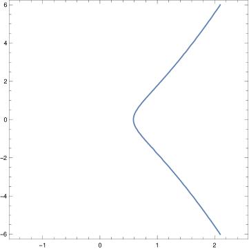
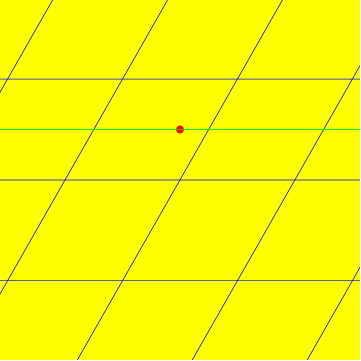
Figure 1. For $c=-1$ and initial condition $\theta_{0}=0.$, and $\theta^{\prime}_{0}=1.$, we get the elliptic curve $y^{2}=4x^{3}-g_{2}x-g_{3}$ with $g_{2}=0.0833333$, and $g_{3}=0.74537$.The lattice is given by $\omega_{1}=3.19248\,+0.i$, and $\omega_{2}=1.59624\,+2.80121i$. The initial point on the curve is $g_{1}=0.\,+1.4006i$. The discriminant is $\Delta=-15.$.

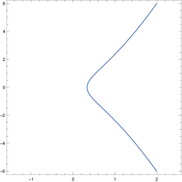
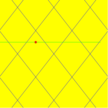
Figure 2. For $c=-1$ and initial condition $\theta_{0}=0.$, and $\theta^{\prime}_{0}=2.$, we get the elliptic curve $y^{2}=4x^{3}-g_{2}x-g_{3}$ with $g_{2}=-2.66667$, and $g_{3}=1.03704$.The lattice is given by $\omega_{1}=1.68575\,+2.15652i$, and $\omega_{2}=-1.68575+2.15652i$. The initial point on the curve is $g_{1}=-1.68575+1.07826i$. The discriminant is $\Delta=-48.$.

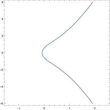
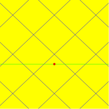
Figure 3. For $c=-1$ and initial condition $\theta_{0}=0.$, and $\theta^{\prime}_{0}=3.$, we get the elliptic curve $y^{2}=4x^{3}-g_{2}x-g_{3}$ with $g_{2}=-3.91667$, and $g_{3}=-0.328704$.The lattice is given by $\omega_{1}=1.91099\,-1.80446i$, and $\omega_{2}=1.91099\,+1.80446i$. The initial point on the curve is $g_{1}=0.\,-0.902231i$. The discriminant is $\Delta=-63.$.

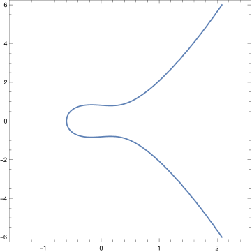
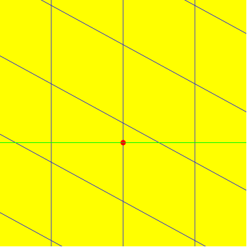
Figure 4. For $c=-1$ and initial condition $\theta_{0}=0.$, and $\theta^{\prime}_{0}=3.9$, we get the elliptic curve $y^{2}=4x^{3}-g_{2}x-g_{3}$ with $g_{2}=0.332008$, and $g_{3}=-0.668123$.The lattice is given by $\omega_{1}=0.\,-3.18149i$, and $\omega_{2}=2.9144\,-1.59074i$. The initial point on the curve is $g_{1}=0.\,-0.795372i$. The discriminant is $\Delta=-12.0159$.

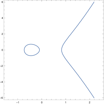
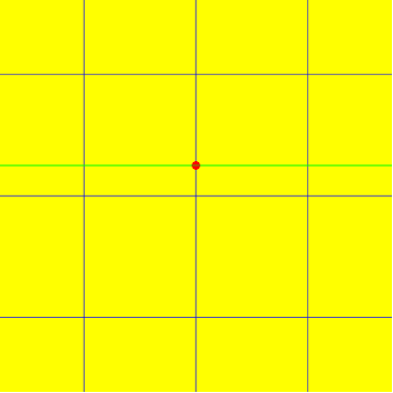
Figure 5. For $c=-1$ and initial condition $\theta_{0}=0.$, and $\theta^{\prime}_{0}=4.1$, we get the elliptic curve $y^{2}=4x^{3}-g_{2}x-g_{3}$ with $g_{2}=2.46801$, and $g_{3}=0.229064$.The lattice is given by $\omega_{1}=2.85478\,+0.i$, and $\omega_{2}=0.\,+3.10293i$. The initial point on the curve is $g_{1}=0.\,+0.775731i$. The discriminant is $\Delta=13.6161$.

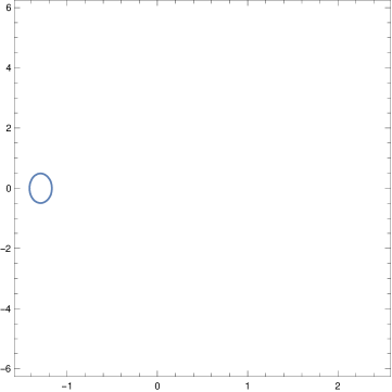
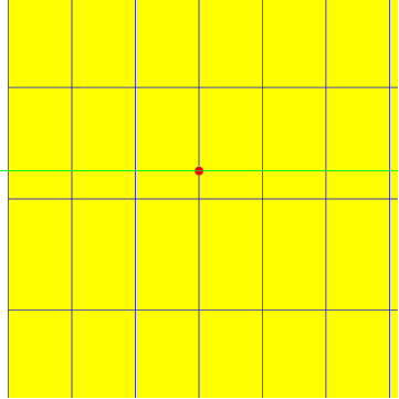
Figure 6. For $c=-1$ and initial condition $\theta_{0}=0.$, and $\theta^{\prime}_{0}=5.$, we get the elliptic curve $y^{2}=4x^{3}-g_{2}x-g_{3}$ with $g_{2}=20.0833$, and $g_{3}=17.0787$.The lattice is given by $\omega_{1}=1.59624\,+0.i$, and $\omega_{2}=0.\,+2.80121i$. The initial point on the curve is $g_{1}=0.\,+0.700302i$. The discriminant is $\Delta=225.$.

Appendix: Mathematica Code

4.6.

Here is an implementation of the solution giving the Weierstrass elliptic function in Mathematica:

⬇

theta0=0.0; thetap0=1; c=-1; e=thetap0^2/2+4*c*Cos[theta0]; b=e/(6c);

a=2c-e^2/(6 c); w0=Exp[I*theta0]; wp0=I*w0*thetap0; w0=w0-b;

g2=-2a; g3=-Chop[wp0^2 + 4*w0^3 + g2*w0]; P=WeierstrassP;

g1=Quiet[(z /. First[Solve[w0==c*P[c*z,{c*g2,g3}],z]]) /. C[1]->0 /. C[2]->0];

z[t_]:=b+c*P[c(t+g1),{c*g2,g3}]; theta[t_]:=Arg[z[t]];

Plot[theta[t], {t, 0, 10}, PlotRange->{-Pi,Pi}]

4.7.

The solution with the Jacobi amplitude function does only plot the trajectory for a half period:

⬇

c=-1; thetap0=1.0;

s=DSolve[{x”[t]==4c*Sin[x[t]],x[0]==0,x’[0]==thetap0},x[t],t];

theta1[T_]:=First[x[t] /. s] /. t->T;

theta1[T_]:=2*JacobiAmplitude[thetap0*T/2,-16/(thetap0^2 c)];

Plot[theta1[t], {t, 0, 10}, PlotRange->{-Pi,Pi}]

4.8.

A numerical solution given by the computer algebra system only gives good values for relatively short time intervals like $t=100$. For longer times, like $t=10^{6}$, the errors in the numerical methods have added up significantly already and the solution has become unreliable. The Weierstrass explicit solution is more convenient.

⬇

c=-1; s=NDSolve[{x”[t]==4c*Sin[x[t]],x[0]==0,x’[0]==1},x[t],{t,0,10^6}];

theta2[T_] := First[x[t] /. s] /. t -> T;

theta[1.0*10^2] - theta2[1.0*10^2]

theta[1.0*10^6] - theta2[1.0*10^6]