Identifiable causal inference with noisy treatment and no side information

Abstract

In some causal inference scenarios, the treatment (i.e. cause) variable is measured inaccurately, for instance in epidemiology or econometrics. Failure to correct for the effect of this measurement error can lead to biased causal effect estimates. Previous research has not studied methods that address this issue from a causal viewpoint while allowing for complex nonlinear dependencies and without assuming access to side information. For such as scenario, this paper proposes a model that assumes a continuous treatment variable which is inaccurately measured. Building on existing results for measurement error models, we prove that our model’s causal effect estimates are identifiable, even without knowledge of the measurement error variance or other side information. Our method relies on a deep latent variable model where Gaussian conditionals are parameterized by neural networks, and we develop an amortized importance-weighted variational objective for training the model. Empirical results demonstrate the method’s good performance with unknown measurement error. More broadly, our work extends the range of applications where reliable causal inference can be conducted.

1 Introduction

Causal inference deals with estimating causal relationships rather than only statistical dependencies, and is thus crucial in fields which seek to make interventions, e.g., medicine or economics [1, 2, 3]. Specifically, causal inference often boils down to the estimation of the distribution of an effect variable $Y$ after an intervention $do(X=x)$ has been applied on a treatment (i.e. cause) variable $X$, which can be calculated using the well-known adjustment formula [1]

$$p(y|do(x))=\int p(y|x,z)p(z)dz,$$ (1)

where $Z$ comprises a set of confounders that satisfy the back-door criterion. (We denote random variables by uppercase letters and their values by the corresponding lowercase letters.) Sometimes the estimation is conditioned on some specific values $Z=z$, resulting in a conditional intervention distribution $p(y|do(x),z)$, which equals $p(y|x,z)$ if $Z$ still satisfies the back-door criterion. In many fields, variables may be subject to noise, e.g., due to inaccurate measurement, clerical error, or self-reporting (often called misclassification for categorical variables). Unaccounted, it is well-known that this error can bias statistical estimates in a fairly arbitrary manner, and, consequently, measurement error models have been widely studied to address this bias [4, 5, 6]. Figure 1 presents an example of this skewing effect. While it is often believed that measurement error only attenuates dependencies, this example demonstrates that on the contrary, dependencies are amplified for some ranges of the treatment variable.

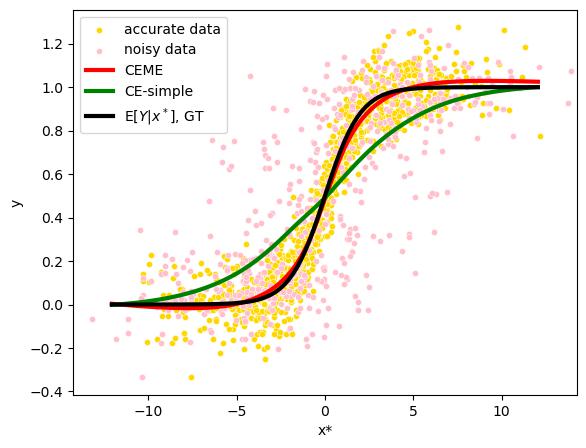
Figure 1: Our method (CEME) compared against regression that assumes the data with noisy measurements of $x^{*}$ is accurate (CE-simple), and against the ground truth (GT) regression function, which is the sigmoid $S(x)=1/(1+e^{-x})$. The accurate values of $x^{*}$ are hidden from both methods and in this example there is no confounding. A similar example is presented in [7].

There is recent, fairly rich literature on the bias introduced by measurement error on causal estimation [4]. It includes qualitative analysis by encoding assumptions of the error mechanism into a causal graph [8], and quantitative analysis of noise in the treatment [7], outcome [9], confounders [10, 11] and mediators [12]. However, almost all of this literature focuses on simple parametric models, such as the linear model, and the identifibility of the causal effect is achieved through side information, such as a known error mechanism, repeated measurements, instrumental variables, or a gold standard sample of accurate measurements. Exceptions include [11] which studies confounder measurement error with no side information and a semiparametric model, and [7] which studies treatment measurement error with a nonparametric model and notably even allowing for unobserved confounding, but utilizes both repeated measurements and an instrumental variable as side information. Thus, there is a gap in the causal inference literature for the challenging case when there is measurement error in the treatment, the amount of noise is unknown, dependencies between variables are complex and non-linear, and no side-information is available to aid in the estimation of the treatment. Our work fills this gap by providing a method for causal inference under these conditions.

We assume that the causal relationships between the variables are depicted in Figure 2, such that the causal effect of interest becomes

$$p(y|do(x^{*}))=\int p(y|z,x^{*})p(z)dz.$$ (2)

The difference between (1) and (2) is that in the latter the true treatment, denoted by $X^{*}$, is hidden, and only a noisy version of it is observed. Without further assumptions, this causal effect is not identifiable because we have no quantitative information of the relationship between $X^{*}$ and the other variables. Therefore, for identification we rely on additional assumptions on the measurement error process $p(x|x^{*})$, such that the conditional distribution $p(y|z,x^{*})$ becomes statistically identifiable, allowing us to compute (2).

Figure 2: Causal graph (and Bayesian network) for our model. Observed variables $X$ (noisy treatment), $Y$ (effect/outcome), and $Z$ (confounders) are shaded to distinguish them from the hidden variable $X^{*}$ (true treatment).

First, we assume that the measurement error is strongly classical, i.e. the observed treatment $X$ is obtained as

$$X=X^{*}+\Delta X,$$

where the measurement error $\Delta X$ is independent of all other variables except $X$, and has a zero mean. Similarly, we assume for the outcome $Y$ that

$$Y=\mu_{Y}(Z,X^{*})+\Delta Y,$$

where the noise $\Delta Y$ is independent of all other variables except $Y$ and has a zero mean. The conditional mean of $Y$, $\mu_{Y}(z,x^{*})={\mathbb{E}}[Y|Z=z,X^{*}=x^{*}]$, is a deterministic function.

Although not strictly necessary for identifiability [13], we further assume Gaussian distributions to facilitate practical computations, yielding

$$X^{*}|Z \sim{\mathbb{N}}(\mu_{X^{*}}(Z),\sigma^{2}_{X^{*}}(Z)),$$ (3)

$$\Delta X \sim{\mathbb{N}}(0,\tau^{2}),$$

$$\Delta Y \sim{\mathbb{N}}(0,\sigma^{2}).$$

We assume that $X$, $Y$, and $X^{*}$ are real-valued scalars, although multivariate extensions are relatively straightforward. The binary (or categorical) case is briefly discussed in Section 2.3.2. The covariate $Z$ can be a combination of categorical, discrete or continuous variables, but the other variables are assumed continuous. Consequently, the learnable parameters are the variance parameters $\tau^{2}$ and $\sigma^{2}$ as well as the (deterministic) functions $\mu_{X^{*}}$, $\sigma_{X^{*}}$ and $\mu_{Y}$, which are all parameterized by neural networks to allow flexible dependencies between the variables.

We note that our model explicitly assumes measurement error only for the treatment variable $X^{*}$, and not for the covariate $Z$ or the outcome $Y$. Implicitly however, measurement error in $Y$ is already included in the noise variance $\sigma^{2}$ because adding Gaussian error simply increases the variance of the original Gaussian noise. To put it in another way, noise in the outcome does not bias the estimation of the dependency between $Y$ and $X$. On the other hand, measurement error in the covariates could also be relevant, but is restricted outside the scope of this work.

Our goal is to study the identifiability of the causal effect in the presence of measurement error. Identifiability terminology can be misleading due to multiple related concepts. We use the following definition:

Definition 1 (Identifiability of an estimand).

Let $P_{X,Z}^{\theta}$ be a probability distribution of the observed variables $X$ and latent variables $Z$, parameterized by $\theta\in\Theta$. Denote by $P^{\theta}_{X}$ the corresponding marginal distribution for $X$. Then an estimand $f(\theta)$ (where $f$ is a deterministic function) is identifiable if for every $\theta,\theta^{\prime}\in\Theta$ we have

$$P^{\theta}_{X}=P^{\theta^{\prime}}_{X}\Rightarrow f(\theta)=f(\theta^{\prime}).$$

As a special case when $f(\theta)=\theta$ we get the definition of model identifiability. Intuitively these mean that knowing the distribution of the observed variables, for example by having estimated it with an infinite amount of i.i.d. samples, the estimand $f(\theta)$ (or simply $\theta$) can be uniquely determined.

In summary, this work contributes to the literature in the following ways:

Theoretical analysis of the identifiability of the causal effect with a noisy treatment, no side information, and complex nonlinear dependencies. We review literature on the identifiability of measurement error models and deep latent variable models, highlighting bridges between disciplines, e.g., econometrics, statistics, machine learning, and apply these results to prove the identifiability of our model.

We formulate a deep latent variable model for estimating the causal effect with measurement error. Experiments with a similar model have been performed in [14], however, they assumed that the error variance was known, which is at least as strong an assumption as having side information, which we want to avoid. We extend previous models by estimating the variance of the measurement error, and demonstrate that importance-weighted amortized variational training can efficiently fit the model while avoiding problems such as posterior collapse.

Empirical demonstrations of the benefits of accounting for measurement error with analyses of artificial and semi-synthetic data.

2 Methods

2.1 Models for causal estimation

In this section we introduce and name the models that we consider for causal estimation in our experiments.

CEME:

Causal Effect estimation with Measurement Error. This is the model defined in Section 1. The mean and standard deviation functions $\mu_{X^{*}}(Z)$, $\sigma_{X^{*}}(Z)$ and $\mu_{Y}(Z,X^{*})$ are fully connected neural networks.

CEME⁺:

Causal Effect estimation with Measurement Error with known noise. This is otherwise the same as CEME, except that here the variance of the measurement error $\sigma^{2}$ is assumed known.

CE-oracle:

This method assumes the model in Figure 3(a), where the true treatment $X^{*}$ is observed and is used directly to estimate the causal effect using (2). Hence, this model provides a loose upper bound on the performance that can be achieved by the models CEME and CEME⁺ which only observe the noisy treatment $X$. The model consists of only one neural network, parametrizing $\mu_{Y}(Z,X^{*})$.

CE-simple:

This is the same as CE-oracle, except that it naively uses the observed noisy treatment $X$ in place of the true treatment $X^{*}$ when estimating the causal effect (model depicted in Figure 3(b)). Hence, it provides a baseline that corresponds to the usual approach of neglecting the measurement error in causal estimation. The model consists of only one neural network, parametrizing $\mu_{Y}(Z,X)$.

For inference, CEME and CEME⁺ use amortized variational inference to estimate the latent variable (described in the next section). On the other hand, CE-oracle and CE-simple, which do not have latent variables, are trained using gradient descent with mean squared error (MSE) loss for predicting $Y$.

(a) Causal graph assumed by CE-oracle, which has access to the true treatment $X^{*}$, unlike the other methods.

(b) Causal graph (incorrectly) assumed by CE-simple.

2.2 Inference

Amortized variational inference (AVI) [16] can be used to estimate the parameters of deep latent variable models (LVMs). Let $X^{*}$ denote the latent variable (e.g. the true treatment in our model) and $S$ all observed variables. First, we define a generative model for the joint distribution $p(S,X^{*})$, also called a decoder, and a model for the posterior $p(X^{*}|S)$, also called an encoder. We optimise the parameters of these models with stochastic gradient descent using the negative evidence lower bound (ELBO, defined in the next section) as the loss function. This approach can be used for LVMs that generalize the variational autoencoder (VAE) to more than just one hidden and one observed node [17]. (CEME/CEME⁺ uses the Bayesian network in Figure 2.) We use AVI conditioned on another observed variable $Z$ (i.e. the confounder in our case), in which case we learn models for $p(S,X^{*}|Z)$ and $p(X^{*}|S,Z)$. Finally, the causal effect estimates of interest can be calculated from the generative model parameters by Monte Carlo sampling over observed covariates $Z$.

As the generative model $p_{\theta}(x^{*},x,y|z)$, we use the model defined in Section 1, parametrized by fully connected neural networks. The generative model parameters also include the scalar variances $\tau$ and $\sigma$, and are jointly denoted by $\theta$. The posterior of $X^{*}$ is approximated by the encoder as follows:

$$p(X^{*}|Z,X,Y) \approx q_{\phi}(X^{*}|Z,X,Y)$$ (4)

$$={\mathbb{N}}\left(X^{*}|\mu_{q}(Z,X,Y;\phi),\sigma_{q}(Z,X,Y;\phi)\right),$$

where again the functions $\mu_{q}(Z,X,Y;\phi)$ and $\sigma_{q}(Z,X,Y;\phi)$ are parametrized by fully connected neural networks and $\phi$ denotes all encoder parameters.

2.2.1 Model training

As our objective function, we use the importance weighted ELBO $\mathcal{L}_{k}$ [15], which is a lower bound for the conditional log-likelihood $p_{\theta}(x,y|z)$:

$$\log p_{\theta}(\mathbf{x,y|z}) =\sum_{i=1}^{N}\log p_{\theta}(x_{i},y_{i}|z_{i})$$ (5)

$$=\sum_{i=1}^{N}\log{\mathbb{E}}\left[\frac{1}{K}\sum_{j=1}^{K}w_{i,j}\right]$$ (6)

$$\geq\sum_{i=1}^{N}{\mathbb{E}}\left[\log\frac{1}{K}\sum_{j=1}^{K}w_{i,j}\right]$$ (7)

$$:=\mathcal{L}_{K},$$ (8)

where $w_{i,j}=p_{\theta}(z_{i},x^{*}_{i,j},x_{i},y_{i})/q_{\phi}(x^{*}_{i,j}|z_{i},x_{i},y_{i})$ are the so-called importance weights, and the expectations are with respect to $q_{\phi}(x^{*}_{i,j}|z_{i},x_{i},y_{i})$. The inequality in (7) is obtained by applying Jensen’s inequality. The standard ELBO corresponds to $k=1$. For practical optimization, the expectation in Equation (7) is estimated by sampling the $K$ importance weights $w_{i,j}$ once per data point $i$.

We use the importance weighted ELBO instead of the standard ELBO, because the latter places a heavy penalty on posterior samples not explained by the decoder, which forces a bias on the decoder to compensate for a misspecified encoder [17]. Increasing the number of importance samples alleviates this effect, and in the limit of infinite samples, decouples the optimization of the decoder from that of the encoder. To calculate the gradient of the ELBO, it is standard to use the reparameterization trick, meaning that we sample $x_{i,j}^{*}|z_{i},x_{i},y_{i}\sim q_{\phi}(x_{i,j}^{*}|z_{i},x_{i},y_{i})$ as

$$x_{i,j}^{*}=\epsilon\cdot\sigma_{q}(z_{i},x_{i},y_{i};\phi)+\mu_{q}(z_{i},x_{i},y_{i};\phi),$$ (9)

where $\epsilon$ follows the standard normal distribution.

Amortized variational inference is prone to getting stuck at local optima, for example in the case of the so-called posterior collapse [17]. To counter this, we start training with an increased but gradually annealed weight for the ELBO terms $\log q_{\phi}(x^{*}_{i,j}|s_{i})$ and $\log p_{\theta}(x_{i}|x^{*}_{i,j})$, which causes the model to initially predict posterior $x^{*}$ close to $x$, to ensure the posterior does not get stuck at the prior. A related approach was taken in [14], where the model was pre-trained assuming no measurement error. The importance weighted ELBO objective is optimized using the Adam gradient descent. Further training details are available in Appendix A. The algorithm was implemented in PyTorch, with code available for replicating the experiments at https://github.com/antti-pollanen/ci_noisy_treatment.

2.3 Identifiability analysis

2.3.1 Identifiability of causal estimation with a noisy treatment

The identifiability proof of our model introduced in Section 1 builds on an earlier result in [13], of which we provide an overview here. The exact form is included in Appendix B. The result concerns scalar real-valued random variables $Y,X^{*},X,\Delta X$ and $\Delta Y$ related via

$$Y=g(X^{*})+\Delta Y\quad\text{and}\quad X=X^{*}+\Delta X,$$ (10)

where only $X$ and $Y$ are observed. We assume that 1) $X^{*},\Delta X$ and $\Delta Y$ are mutually independent, 2) ${\mathbb{E}}[\Delta X]={\mathbb{E}}[\Delta Y]=0$, and 3) some fairly mild regularity conditions. This model differs from ours in that it does not include the covariate $Z$, but on the other hand it is more general in that it does not assume that $X^{*},\Delta X$ and $\Delta Y$ are (conditionally) Gaussian. It is shown in [13] that this model is identifiable if the function $g$ in Equation (10) is not of the form

$$g(x^{*})=a+b\ln(e^{cx^{*}}+d),$$ (11)

and even if it is, nonidentifiability requires $x^{*}$ to have a specific distribution, e.g. a Gaussian when $g$ is linear. Based on this, we are now ready to prove the following proposition and corollary that establish the identifiability of the CEME model:

Proposition 1.

The measurement error model in Section 1 is model identifiable if 1) for every $z$, $\mu_{Y}(z,x^{*})$ is continuously differentiable everywhere as a function of $x^{*}$, 2) for every $z$, the set $\chi=\{x^{*}:\frac{\partial}{\partial x^{*}}\mu_{Y}(z,x^{*})=0\}$ has at most a finite number of elements, and 3) there exists $z$ for which $\mu_{Y}(z,x^{*})$ is not linear in $x^{*}$ (i.e. of the form $\mu_{Y}(x^{*})=ax^{*}+b$).

Proof.

The full proof is provided in Appendix C, but its outline is the following: First, we show that a restricted version of our model where $z$ can only take one value is identifiable as long as $\mu_{Y}(z,x^{*})$ is not linear in $x^{*}$. This follows from the identifiability theorem in [13] because its assumptions are satisfied by the restricted version of our model, together with the assumptions of Proposition 1.

Second, we show the identifiability of our full model by looking separately at values of $z$ for which $\mu_{Y}(z,x^{*})$ is or isn’t linear in $x^{*}$. For the model conditioned on the latter type of $z$ (nonlinear cases), identifiability was shown in the first part of the proof. For the remaining linear cases, we use the fact that we already identified $\tau$ and $\sigma$ with the nonlinear cases, which results in a linear-Gaussian model with known errors, which is known to be identifiable (see e.g. [18]). Thus the whole model is identified. ∎

We note that assumption 1) in Proposition 1 is satisfied by the neural networks used in this work, as they are continuously differentiable due to using the extended linear unit (ELU) activation function. Assumption 2) is true in general, and does not hold only in the special case where the derivative of the neural network $\mu_{Y}(z,x^{*})$ is zero with respect to $x^{*}$ in infinitely many points, which is possible only if the function is constant on an interval. Breaking assumption 3) would require the network $\mu_{Y}(z,x^{*})$ to be linear in $x^{*}$ for every $z$. Even when this is the case, we still hypothesise that the model is identifiable as long as there are multiple values of the linear slope for different $z$. This is suggested by solving a system of equations similar to [18], which appears to have one or at most two distinct solutions. We leave a detailed investigation of this case for future work.

Finally, the identifiability of the causal estimands of interest is shown by the following corollary:

Corollary 1.

The causal estimands $p(y|do(x^{*}))$ and $p(y|do(x^{*}),z)$ are identifiable for the model in Section 1 if assumptions 1), 2) and 3) of Proposition 1 are satisfied and the variables in $Z$ satisfy the backdoor criterion w.r.t $X^{*}$ and $Y$.

Proof.

Since the model in Section 1 is shown identifiable in Proposition 1, we have that for every combination of $\theta_{1}$ and $\theta_{2}$, $P^{\theta_{1}}_{Z,X,Y}=P^{\theta_{2}}_{Z,X,Y}$ implies $\theta_{1}=\theta_{2}$. Since the causal effects $p_{\theta}(y|do(x^{*}))$ and $p_{\theta}(y|do(x^{*}),z)$ are functions of the joint distribution $P^{\theta}_{Z,X,X^{*},Y}$ which in turn is a function of $\theta$, we obtain from $\theta_{1}=\theta_{2}$ that $p_{\theta_{1}}(y|do(x^{*}))=p_{\theta_{2}}(y|do(x^{*}))$ and $p_{\theta_{1}}(y|do(x^{*}),z)=p_{\theta_{2}}(y|do(x^{*}),z)$. ∎

2.3.2 Related identifiability literature

CEME with categorical variables. Identifiability is proven in [19] for a model with the same Bayesian networks as ours (Figure 2) where the treatment $X^{*}$ and covariate $Z$ are categorical. For this result, misclassification probabilities need to have a certain upper bound to avoid the label switching problem. It is also assumed that the conditional distribution $Y|Z,X^{*}$ is either a Poisson, normal, gamma or binomial distribution. This scheme also allows dealing with missing treatment values by defining a missing value as an additional category.

Measurement error models from a statistical perspective. There is a wide variety of research on measurement error solely from a statistical (non-causal) perspective, studying assumptions under which measurement error model parameters can be identified, and exploring different practical methods for inferring them. These include the general method of moments (GMM) as well as kernel deconvolution and sieve estimators [4, 6]. Many of our assumptions are relaxed, such as having the Gaussian noise terms, the independence of the measurement error $\Delta X$ or outcome noise $\Delta Y$ of the other variables, and the outcome $Y$ being non-differential, i.e. independent of $\Delta X$. See [5, 6] for a review on this type of results.

A wide variety of literature also studies measurement error models with additional assumptions compared to ours. These consist mainly of assuming availability of side information such as repeated measurements or instrumental variables (IVs), or assuming a strict parametric form (e.g. linear or polynomial) for the regression function ${\mathbb{E}}[Y|Z,X^{*}]$ (and ${\mathbb{E}}[X^{*}|Z]$). See [4] for a review. The IVs differ from our covariate $Z$ in that the IV is conditionally independent of $Y$ given $X^{*}$. On the other hand, [20] considers a covariate $Z$ that directly affects $Y$, however they assume that the effects of $Z$ and $X^{*}$ on $Y$ are either decoupled or ${\mathbb{E}}[Y|Z,X^{*}]$ has a polynomial parametric form.

Related latent variable models. There are also latent variable models studied that resemble the measurement error model. These include the causal effect variational autoencoder (CEVAE) where only a proxy of the confounder is observed [21, 22] and nonlinear independent component analysis [23]. Also [5, 6] consider the identification of latent variable models more generally.

3 Experiments and results

We conduct two experiments: One with datasets drawn from Gaussian processes, where a large number of datasets is used to establish the robustness of our results. Second, we use an augmented real-world dataset on the relationship between years of education and wage, to study the effect of complex real-world patterns for which the assumptions of our model do not hold exactly.

3.1 Synthetic experiment

3.1.1 Synthetic datasets from Gaussian processes

For the synthetic experiment, we generate datasets which follow the model defined in Section 1 where all variables are scalars, and the covariate $Z$ is sampled from the standard Gaussian. The functions $\mu_{X^{*}}$, $\sigma_{X^{*}}$ and $\mu_{Y}$ are sampled from a Gaussian process (GP), once per dataset. The Gaussian process has a zero mean and uses a squared exponential kernel (also known as the radial basis function kernel)

$$k(x_{1},x_{2})=\alpha\exp\left(-\frac{|x_{1}-x_{2}|^{2}}{2l^{2}}\right)$$

with $\alpha=1$ and lengthscale $l=2$. The functions $\mu_{X^{*}}$, $\sigma_{X^{*}}$ and $\mu_{Y}$ are only approximately generated from a GP to limit the size of the kernel which would otherwise grow proportionally to the square of the number of data points. The exact procedure to generate the data as well as further experimental details are available in Appendix A. The measurement error $\tau$ and outcome noise $\sigma$ are set as

$$\tau=l\sqrt{\mathrm{Var}[X^{*}]},$$ (12)

$$\sigma=l\sqrt{\mathrm{Var}[\mu_{Y}(Z,X^{*})]},$$ (13)

where the noise level $l$ is a constant that equals either $l=0.1$ (small noise), $l=0.2$ (medium noise) or $l=0.4$ (large noise). Three datasets generated in this way are shown in Figure 4.

Figure 4: Three realizations of synthetic datasets generated from a Gaussian process with 3000 data points (black dots). The figures show the covariate $Z$ (x-axis), and the noiseless versions of the treatment $X^{*}$ (y-axis) and the outcome ${\mathbb{E}}[Y|Z,X^{*}]$ (heatmap).

We run experiments for three training dataset sizes, 1000, 4000 and 16000. The test set consists of 20000 data points. We run each experiment on 200 datasets generated in the same way but sampled from a different distribution. Each dataset is analysed 6 times and the run with the best score on a separate validation dataset is included in the results. All algorithms (CEME, CEME⁺, CE-simple and CE-oracle) use the same neural network architecture to facilitate a fair comparison, i.e. three fully connected hidden layers with 20 nodes each, and the ELU activation function.

3.1.2 Results

The individual causal effect $p(y|z,do(x^{*}))=p(y|z,x^{*})=\mathcal{N}(y|\mu_{Y}(z,x^{*}),\sigma^{2})$ is for this experiment completely characterized by $\mu_{Y}(z,x^{*})={\mathbb{E}}[Y|z,do(x^{*})]$ and $\sigma^{2}=\mathrm{Var}[Y|z,do(x^{*})]$. Therefore, we assess the accuracy of the individual causal effect by measuring accuracy of ${\mathbb{E}}[Y|z,do(x^{*})]$ and $\mathrm{Var}[Y|z,do(x^{*})]$. The former is reported in Figure 5 using the root mean squared error

$$\sqrt{\mathrm{MSE}}=\sqrt{\sum_{i=1}^{N}(\mu_{Y,\theta}(z_{i},x^{*}_{i})-\mu_{Y}(z_{i},x^{*}_{i}))^{2}},$$

where $\theta$ denotes the estimate. The accuracy of estimation of $\mathrm{Var}[Y|z,do(x^{*})]$ is reported in Figure 6, which uses as metric relative error $(\sigma_{\theta}-\sigma)/\sigma$. Similarly, the relative error in the estimation of the measurement error noise $\tau$ is reported in Figure 8. The accuracy in estimation of $p(y|do(x^{*}))$ is assessed using Average Interventional Distance (AID) [22]:

$$\mathrm{AID} =\int p(x^{*})\int\mid p_{\theta}(y|do(x^{*}))-p(y|do(x^{*}))\mid dydx^{*}$$ (14)

$$\approx\frac{1}{N}\sum_{i=1}^{N}\int\mid p_{\theta}(y|do(x^{*}_{i}))-p(y|do(x^{*}_{i}))\mid dy.$$

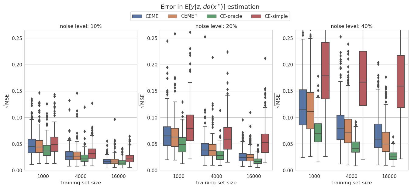
Figure 5: Error in ${\mathbb{E}}[y|z,do(x^{*})]$ estimation in the synthetic experiment. Besides data for CE-simple, missing from the figure are some outliers for CEME and CEME⁺ for noise level 40% and training dataset size 1000.

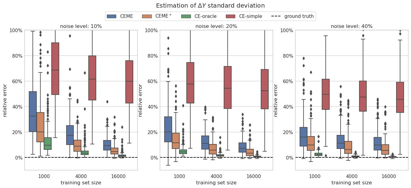
Figure 6: Error in estimation of $\Delta Y$ standard deviation in the synthetic experiment. Besides data for CE-simple, missing from the figure are 4 outliers for CEME, 1000 training data and 10% noise as well as 2 outliers for CEME, 4000 training data and 10% noise.

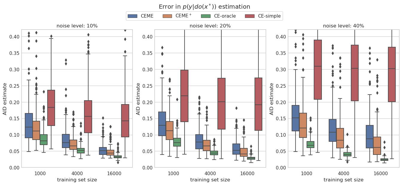
Figure 7: Error in estimation of $p(y|do(x^{*}))$ in the synthetic experiment. Besides data for CE-simple, missing from the figure are 3 outliers for CEME and 1 for CEME⁺, both for 40% noise and 1000 training data.

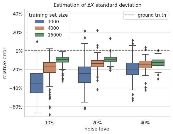
Figure 8: Error in estimation of $\Delta X$ standard deviation by CEME in the synthetic experiment.

In these figures, the data is represented as boxplots, where the box corresponds to the interquantile range, with the median represented as a horizontal bar. The whiskers extend to the furthest point within their maximum length, which is 1.5 times the interquantile range. Outliers beyond the whiskers are represented as singular points. Each datapoint corresponds to a separate data generating distribution and the best of six runs based on validation loss.

We observe that overall the CEME algorithms offer significant benefit over not taking measurement error into account at all (algorithm CE-simple), both in terms of estimating individual causal effect (Figures 5 and 6), and average causal effect (Figure 7). Also, the results seem to suggest convergence of estimates when increasing dataset size, in accordance with Corollary 1. On the other hand, even with knowledge of the true standard deviation (SD) of $\Delta X$, CEME⁺ does not achieve comparable performance to CE-oracle. This is to be expected as CE-oracle sees the accurate values of $X^{*}$ for individual datapoints, which cannot be identified even in principle from information available to CEME and CEME⁺.

Interestingly, the performance improvement from knowing the true SD of $\Delta X$ (with CEME⁺) over learning it (with CEME) seems relatively modest. This suggests that identifiability is in general not an issue for CEME, even though the data distributions could be arbitrarily close to the non-identifiable linear-Gaussian case. We also note that all algorithms almost always overestimate the SD of $\Delta Y$, which could be explained by an imperfect regression fit. Furthermore, as detailed in Section 2.2.1, the training of CEME and CEME⁺ is initialized such that they try to predict $X^{*}$ close to $X$, which could be another cause for this and also explain why CEME tends to underestimate the SD of $\Delta X$ (Figure 8).

3.2 Experiment with education-wage data

We also test CEME with semisynthetic data based on a dataset curated in [24] from data from the National Longitudinal Survey of Young Men (NLSYM), conducted between years 1966 and 1981. The items in the dataset correspond to persons, whose number of education years is used as treatment $X^{*}$. As outcome $Y$, we use the logarithm of wage. The relationship between these is also studied in the original paper [24]. The dataset also contains multiple covariates, of which we use a total of 23, including age, whether the person was living with their mom and/or dad at the age of 14, if the person is living near colleges, binary variables specifying in what region the person is living in, and whether they had access to a library card at the age of 14.

We leave out multiple covariates present in the original dataset that correlate heavily with the number of education years and would thus make measurement error correction for it much less useful. These include the education status of the person’s mother and father, their intelligence quotient, Knowledge of the World of Work (KWW) score and work experience in years. More details on what covariates were used and which dropped are available in Appendix A. Missing values are handled by dropping all data items that contain them. This brings down the size of the dataset from 3010 to 2990.

In addition, we take several steps to modify and augment the dataset for the purpose of testing CEME/CEME⁺. Firstly, both $X^{*}$ (number of education years) and all covariates in $Z$ are scaled to have a zero mean and unit variance. The noisy treatment $X$ is obtained by adding a normally distributed additive noise $\Delta X$ to $X^{*}$. Six separate datasets are created, each corresponding to a different level of SD of $\Delta X$. The levels are proportional to the SD of $X^{*}$, and are 0%, 20%, 40%, 60%, 80% and 100%.

We choose the number of education years as the true treatment variable $X^{*}$ because we want to accurately know the ground truth to be able to evaluate our method. This would not be possible if we chose a variable that is actually inaccurate in the real world, despite it making more sense in terms of a real world application of our model.

A synthetic outcome $Y$ is generated as follows based on the true value of the logarithm of wage: First, we train a neural network (five hidden layers of size 30, weight decay 0.01 and ELU activation function) to predict the logarithm of wage (scaled to have zero mean and unit variance). Then we use the trained neural network as the function $\mu_{Y}[Z,X^{*}]={\mathbb{E}}[Y|Z,X^{*}]$. To obtain $Y$, we add to this expectation a Gaussian noise $\Delta Y$ whose SD is set to 10% of the true SD estimated with training data for the $\mu_{Y}[Z,X^{*}]$ neural network. This neural network was trained on all the data items, but was regularized not to overfit to a meaningful extent. The SD is only 10% of the estimated true SD, because otherwise the predictions are so inaccurate to begin with that better handling of measurement error has little potential to improve results. The synthetic $Y$ is also used as the ground truth for ${\mathbb{E}}[Y|Z,X^{*}]$.

The CEME/CEME⁺ models are actually misspecified for this dataset because the true treatment, the number of education years, is ordinal, instead of conditionally Gaussian like the models assume. This presents an opportunity to evaluate the sensitivity of the CEME/CEME⁺ algorithms to model misspecification.

We run this experiment for the same four algorithms as in the synthetic experiment, defined in Section 2.1, with three hidden layers of width 26 and the ELU activation function. The training procedure and model structures are the same as in Section 3.1 expect that now $Z$ is multivariate and hyperparameters are different, as detailed in Appendix A. The full data of 2990 points is split into 72% of training data, 8% of validation data (used for learning rate annealing and early stopping) and 20% of test data (rounded to the nearest integer). The code used for data preprocessing and running the experiment is available at https://github.com/antti-pollanen/ci_noisy_treatment.

3.2.1 Results

The main results in the experiment with education-wage data are presented in Figures 9(a), 9(b), 10(a) and 10(b). They use the same metrics as the corresponding results for the synthetic data experiment. The points represent median values and the bands interquantile ranges. Each datapoint corresponds to one training run of the model, and the x-axis in each figure tells which dataset was used (they differ only in the SD of the augmented noise $\Delta X$). There is no entry for CEME⁺ for the 0% $\Delta X$ SD dataset, because using variational inference for a model with no hidden variables is not useful and is problematic in practice due to terms in the ELBO becoming infinite.

We notice that while CEME and CEME⁺ still offer a clear improvement over not accounting for measurement at all (CE-simple), they seem to be further below in performance from CE-oracle (which acts as a benchmark for optimal, or even beyond-optimal performance for the CEME/CEME⁺ algorithms). A potential reason for this is that the CEME models, which model the true number of education years as a continuous latent variable, are misspecified unlike CE-oracle and CE-simple, which only condition on the number of education years but do not model it (though CE-simple assumes that there is no measurement error). Moreover, CEME and CEME⁺ have more parameters than CE-oracle and CE-simple, so they could be hurt more by the limited dataset size and high-dimensional covariate. The larger difference between CEME and CEME^∗ than in the synthetic experiment might be due to the fact that CEME^∗ avoids some of the detriments from model misspecification, by having access to the true SD of $\Delta X$.

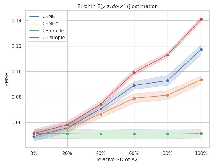
(a) Error in ${\mathbb{E}}[Y|Z=z,do(X^{*}=x^{*})]$ estimation.

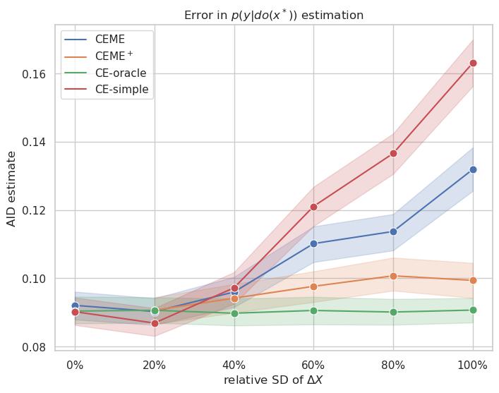
(b) Error in $p(y|do(x^{*}))$ estimation.

Figure 9: Error in causal effect estimation in the education-wage data experiment.

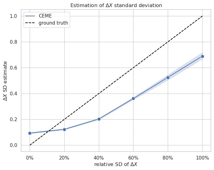
(a) Estimation of $\Delta X$ standard deviation.

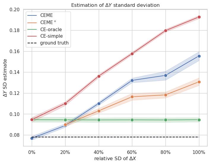
(b) Estimation of $\Delta Y$ standard deviation.

Figure 10: Error in estimation of treatment and outcome noises in the education-wage data experiment.

4 Conclusion

In this work, we provided a model for causal effect estimation in the presence of treatment noise, with complex nonlinear dependencies, and with no available side information. We confirmed the model’s identifiability theoretically and evaluated it experimentally, comparing it to a baseline of not accounting for measurement error at all (CE-simple) and to an upper bound in performance in the form of CE-oracle. A notable advantage of the model is its flexibility: It offered good performance on a diverse set of synthetic datasets and was useful for correcting for measurement error even on a real-world dataset for which it was somewhat misspecified.

A limitation of the CEME/CEME⁺ methods is their assumption of independent additive noise for both treatment and outcome, which might not always hold [5]. On the other hand, these assumptions were critical for attaining identifiability without side information, so relaxing them would likely mean having to introduce side information to the model [6]. Another limitation of our study is the lack of comparison to other state-of-the-art methods. However, the authors are not aware of any that exist for the setting where the treatement is noisy, the regression function does not have any strict parametric form, the model is conditioned on a covariate, and no side information is available. Also, our study does not consider the robustness of estimation when there is no access to a perfect set of covariates satisfying the backdoor criterion.

Finally, the model is limited by assuming conditionally Gaussian distributions throughout the model. An interesting direction for future research could be to relax this assumption by using a flexible model, such as normalizing flows, for these densities. The identifiability result in [13] suggests a model generalized in this way would retain its identifiability. Also, since it is straightforward to generalize the amortized variational approach of this work for other related latent variable models, an interesting future direction of research could be to try the approach for any scenarios which relax the classical measurement error assumptions of this work [5, 6] and where flexible efficient methods for inference are not yet available.

Appendix

Appendix A Experiment details

A.1 Synthetic experiment

In the synthetic experiment data generation, the functions $\mu_{X^{*}}$, $\sigma_{X^{*}}$ are only approximately sampled from a GP to save in computation cost, as with exact values the size of the GP kernel scales proportionally to the square of the number of data points, and the matrix operations performed with it scale even worse. Thus, we sample only $K=1000$ points from the actual Gaussian processes corresponding to each of the functions $\mu_{X^{*}}$, $\sigma_{X^{*}}$ and $\mu_{Y}$. These functions are then defined as the posterior mean of the corresponding GP, given that the $K$ points have been observed. The points are evenly spaced so that the minimum is the smallest value in the actual generated data minus one quarter of the distance between the smallest and largest value in the actual data. Similarly, the maximum is the largest value in the actual data plus the distance between the smallest and largest value in the actual data. This is achieved by generating the actual values ${z_{i}}_{i=1..N}$ first, then sampling the $K$ points for $\mu_{X^{*}}$, and $\sigma_{X^{*}}$, then generating $x^{*}_{i=1..N}$ and then finally sampling the $K$ points for $\mu_{Y}$.) For $\mu_{Y}$, as it has two arguments, we used $K=31^{2}=961$ points arranged in a two-dimensional grid.

When training the model, learning rate annealing is used, which means that if there has been a set number of epochs without validation score improving, learning rate will be multiplied by a set learning rate reduction factor. The training is stopped when a set amount of epochs has passed without validation score improving.

Hyperparameter values used are listed in Table 1. They were optimized using a random parameter search. We use 8000 data points as the validation set used for annealing learning rate as well as for early stopping. Unless otherwise stated, the same hyperparameter value was used for all algorithms and all datasets. From all the 43200 runs in the synthetic experiment, only 33 runs crashed yielding no result.

Hyperparameter	Value
Weight decay	0
Number of importance samples	32
Initial weight of $\log q_{\phi}(x^{*}_{i,j}|s_{i})$ and $\log p_{\theta}(x_{i}|x^{*}_{i,j})$ terms (see Section 2.2.1)	4
Number of epochs to anneal above weight to 1	10
Learning rate reducer patience	30
Learning rate reduction factor	0.1
Early stopping patience in epochs	40
Adam $\beta_{1}$	0.9
Adam $\beta_{2}$	0.97
Batch size used for CEME/CEME+ when training dataset size is 16000	256
Batch size otherwise	64
Learning rate for CEME/CEME+ with training dataset sizes 1000 and 4000	0.003
Learning rate for CEME/CEME+ with training dataset size 16000	0.01
Learning rate for CE-oracle and CE-simple	0.001

Table 1: Hyperparameter values used in the synthetic experiment.

A.2 Experiment with education-wage data

For the education-wage dataset from [24], the covariates used were personal identifier, whether the person lived near a 2 year college in 1966, whether the person lived near a 4 year college in 1966, age, whether the person lived with both parents or only mother or with step parents at the age of 14, several variables on which region of USA the person lived in, whether the person lived in a metropolitan area (SMSA) in 1966 and/or 1967, whether the person was enrolled in a school in 1976, whether the person was married in 1976, and whether the person had access to a library card at the age of 14.

Covariates dropped from our experiment were mother’s schooling in years, father’s schooling in years, NLS sampling weight, Knowledge of World of Work score (KWW), IQ, work experience in years, its square, work experience years divided into bins, and wage.

Hyperparameter values used are listed in Table 2. The hyperparameters are shared by all the algorithms and were optimized using a random search. A separate search was conducted for each type of algorithm, but the optima were close enough that for simplicity the same values could be chosen for each algorithm.

Hyperparameter	Value
Batch size	32
Learning rate	0.001
Weight decay	0.001
Number of importance samples	32
Initial weight of $\log q_{\phi}(x^{*}_{i,j}|s_{i})$ and $\log p_{\theta}(x_{i}|x^{*}_{i,j})$ terms (see Section 2.2.1)	8
Number of epochs to anneal above weight to 1	5
Learning rate reducer patience	25
Learning rate reduction factor	0.1
Early stopping patience in epochs	45
Adam $\beta_{1}$	0.9
Adam $\beta_{2}$	0.97

Table 2: Hyperparameter values used in the experiment with education-wage data.

Appendix B Identification theorem used to prove Proposition 1

For completeness, we include below Theorem 1 from [13] (repeated mostly word-for-word):

Definition 2.

We say that a random variable $r$ has an $F$ factor if $r$ can be written as the sum of two independent random variables (which may be degenerated), one of which has the distribution $F$.

Model 1. Let $y$, $x$, $x^{*}$, $\Delta x$, $\Delta y$ be scalar real-valued random variables related through

$$y =g(x^{*})+\Delta y$$ (15)

$$x =x^{*}+\Delta x,$$ (16)

and $y$ are observed while all remaining variables are not and satisfy the following assumptions:

Assumption 1. The variables $x^{*}$, $\Delta x$, $\Delta y$, are mutually independent, ${\mathbb{E}}[\Delta x]=0$, and $E[\Delta y]=0$ (with ${\mathbb{E}}[|\Delta x|]<\infty$ and ${\mathbb{E}}[|\Delta y|]<\infty$).

Assumption 2. $E[e^{i\xi\Delta x}]$ and $E[e^{i\gamma\Delta y}]$ do not vanish for any $\xi,\gamma\in{\mathbb{R}}$, where $i=\sqrt{-1}$.

Assumption 3. (i) $E[e^{i\xi x^{*}}]\neq 0$ for all $\xi$ in a dense subset of ${\mathbb{R}}$ and (ii) $E[e^{i\gamma g(x^{*})}]\neq 0$ for all $\gamma$ in a dense subset of ${\mathbb{R}}$ (which may be different than in (i)).

Assumption 4. The distribution of $x^{*}$ admits a uniformly bounded density $f_{x^{*}}(x^{*})$ with respect to the Lebesgue measure that is supported on an interval (which may be infinite).

Assumption 5. The regression function $g(x^{*})$ is continuously differentiable over the interior of the support of $x^{*}$.

Assumption 6. The set $\chi=\{x^{*}:g^{\prime}(x^{*})=0\}$ has at most a finite number of elements $x^{*}_{1},...,x^{*}_{m}$. If $\chi$ is nonempty, $f_{x^{*}}(x^{*})$ is continuous and nonvanishing in a neighborhood of each $x^{*}_{k}$, $k=1,...,m$.

Theorem 1.

Let Assumptions 1-6 hold. Then there are three mutually exclusive cases:

1. $g(x^{*})$ is not of the form

   $$g(x^{*})=a+b\ln(e^{cx^{*}}+d)$$ (17)

   for some constants $a,b,c,d\in{\mathbb{R}}$. Then, $f_{x^{*}}(x^{*})$ and $g(x^{*})$ (over the support of $f_{x^{*}}(x^{*})$) and the distributions of $\Delta x$ and $\Delta y$ in Model 1 are identified.

2. $g(x^{*})$ is of the form (17) with $d>0$ (A case where $d<0$ can be converted into a case with $d>0$ by permuting the roles of $x$ and $y$). Then, neither $f_{x^{*}}(x^{*})$ nor $g(x^{*})$ in Model 1 are identified iff $x^{*}$ has a density of the form

   $$f_{x^{*}}(x^{*})=A\exp(-Be^{Cx^{*}}+CDx^{*})(e^{Cx^{*}}+E)^{-F},$$ (18)

   with $c\in{\mathbb{R}}$, $A,B,D,E,F\in[0,\infty]$ and $\Delta y$ has a Type I extreme value factor (whose density has the form $f_{u}(u)=K_{1},\exp(K_{2}\exp(K_{3}u)+K_{4}u)$ for some $K_{1},K_{2},K_{3},K_{4}\in{\mathbb{R}}$).

3. $g(x^{*})$ is linear (i.e., of the form (17) with $d=0$). Then, neither $f_{x^{*}}(x^{*})$ nor $g(x^{*})$ in Model 1 are identified iff $x^{*}$ is normally distributed and either $\Delta x$ or $\Delta y$ has a normal factor.

Appendix C Proof of Proposition 1

Proof.

First, consider the measurement error model in Section 1 conditioned on a specific value $Z=z$, effectively removing $Z$ as a variable. We show that this model, called the restricted model, as opposed to the original full model, satisfies the assumptions in Theorem 1, which thus determines when the restricted model is identifiable. Firstly, the restricted model satisfies Equations (15) and (16). Assumption 1 follows directly from the definition of the model, as $|\Delta X|$ and $|\Delta Y|$ follow the half-normal distribution, which has the known finite expectation $\sigma\sqrt{2}/\sqrt{\pi}$. Assumption 2 is satisfied because $\Delta X$ and $\Delta Y$ are Gaussian, so their characteristic functions have the known form $\exp(i\mu t-\sigma^{2}t^{2}/2)$ and thus do not vanish for any $t\in{\mathbb{R}}$ ($t$ is denoted by $\xi$ or $\gamma$ in Assumption 2).

Assumption 3 of Theorem 1 is not needed because it is in its proof in [13] only used to find the distributions of the errors $\Delta X$ and $\Delta Y$ given that the density $f_{x^{*}}(x^{*})$ and regression function $g(x^{*})$ are known. However, in our case we already know by assumption that the error distributions are Gaussian with a zero mean, and moreover, we can find their standard deviation from

$$\textrm{Var}[Y]=\textrm{Var}[\mu_{Y}(z,X^{*})]+\textrm{Var}[\Delta Y]$$

and

$$\textrm{Var}[X]=\textrm{Var}[X^{*}]+\textrm{Var}[\Delta X],$$

which hold due to the independence of $\mu_{Y}(z,X^{*})$ and $\Delta Y$ as well as $X^{*}$ and $\Delta X$, respectively. Assumption $4$ is satisfied because $X^{*}|Z=z$ is normally distributed and thus admits a uniformly bounded density w.r.t. the Lebesgue measure that is supported everywhere. Assumption 5 is the same as assumption 1 of our Proposition 1. Assumption 6 follows from assumption 2 of Proposition 1 since the density of $X^{*}|Z=z$ is continuous and nonvanishing everywhere.

With the assumptions of Theorem 1 satisfied, we check what the cases 1-3 therein imply for our restricted model. From case 1 we obtain that it is identified except when $\mu_{Y}(z,x^{*})$ as a function of $x^{*}$ is of the form $a+b\ln(e^{cx^{*}}+d)$.

Case 2 considers the case when $\mu_{Y}(z,x^{*})$ as a function of $x^{*}$ is of the form $a+b\ln(e^{cx^{*}}+d)$ with $d>0$. (Having $d<0$ is impossible as we assume the function $g$ is defined on ${\mathbb{R}}$). In this case, our model is identifiable, as $X^{*}$ is Gaussian and thus its density is not of the form

$$f_{x^{*}}(x^{*})=A\exp(-Be^{Cx^{*}}+CDx^{*})(e^{Cx^{*}}+E)^{-F}$$ (19)

with $C\in{\mathbb{R}}$ and $A,B,D,E,F\in[0,\infty)$. We see this by taking a logarithm of both the Gaussian density and the density in Equation (19) and noting that the first is a second degree polynomial, but the latter is a sum without a second degree term, so they are not equal. Thus our model is identifiable in this case.

The remaining case is for when $\mu_{Y}(z,x^{*})$ is linear in $x^{*}$. In this case, the restricted model is not identified as $x^{*}$ is normally distributed and both $\Delta x$ and $\Delta y$ have normal factors as they are normal themselves.

Next, we prove the identifiability of the full model, i.e. where $z$ may take any value in its range. We start by assuming in accordance with Definition 1 that two conditional observed distributions from the model match for every $z$:

$$\forall z,x,y:\quad p_{\theta}(x,y|z)=p_{\theta^{\prime}}(x,y|z).$$ (20)

Now based on assumption 3 of Proposition 1, there exists $\bar{z}$ for which $\mu_{Y}(\bar{z},x^{*})$ is not linear in $x^{*}$. From (20) we obtain that

$$\forall x,y:\quad p_{\theta}(x,y|\bar{z})=p_{\theta^{\prime}}(x,y|\bar{z}),$$

which in turn implies

$$\tau =\tau^{\prime}$$ (21)

$$\sigma =\sigma^{\prime}$$

$$\mu_{X^{*}}(\bar{z}) =\mu^{\prime}_{X^{*}}(\bar{z})$$

$$\sigma_{X^{*}}(\bar{z}) =\sigma^{\prime}_{X^{*}}(\bar{z})$$

$$\forall x^{*}\in{\mathbb{R}}:\quad\mu_{Y}(\bar{z},x^{*}) =\mu^{\prime}_{Y}(\bar{z},x^{*})$$

by using Definition 1 on the restricted model, which is identified according to the first part of the proof.

In the same manner, we obtain the equalities in (21) for every $\bar{z}$ for which $\mu_{Y}(\bar{z},x^{*})$ is not linear in $x^{*}$. Thus for the full equality of the models (i.e. for $\theta=\theta^{\prime}$), it remains to show that we obtain $\mu_{X^{*}}(z)=\mu^{\prime}_{X^{*}}(z)$, $\sigma^{\prime}_{X^{*}}(z)=\sigma_{X^{*}}(z)$ and $\mu_{Y}(z,x^{*})=\mu^{\prime}_{Y}(z,x^{*})$ also for those $z$ for which $\mu_{Y}(z,x^{*})$ is linear in $x^{*}$. Noting that we now already know that $\tau=\tau^{\prime}$ and $\sigma=\sigma^{\prime}$, we obtain for such $z$ a linear-Gaussian measurement error model with known measurement error, which is known to be identifiable (see e.g. [18]). Thus $\theta=\theta^{\prime}$ and the proof is complete. ∎

References

- [1] Pearl J. Causality. Cambridge University Press; 2009.
- Peters et al. [2017] Peters J., Janzing D., Schölkopf B. Elements of Causal Inference: Foundations and Learning Algorithms. The MIT Press; 2017.
- [3] Imbens G.W., Rubin D.B. Causal Inference in Statistics, Social, and Biomedical Sciences. Cambridge University Press; 2015.
- [4] Yi G.Y., Delaigle A., Gustafson P. Handbook of Measurement Error Models. CRC Press; 2021.
- [5] Schennach S.M. Recent advances in the measurement error literature. Annual Review of Economics. 2016;8:341-77.
- [6] Schennach S.M. Mismeasured and unobserved variables. In: Durlauf S.N., Hansen L.P., Heckman J.J., Matzkin R.L. (Ed.) Handbook of Econometrics. Elsevier; 2020. Vol. 7a, p. 487-565.
- [7] Zhu Y., Gultchin L., Gretton A., Kusner M.J., Silva R. Causal inference with treatment measurement error: a nonparametric instrumental variable approach. In: Cussens J., Zhang K. (Ed.) Proceedings of the Thirty-Eighth Conference on Uncertainty in Artificial Intelligence. PMLR; 2022. p. 2414-24.
- [8] Hernán M.A., Robins J.M. Causal Inference: What If. Boca Raton: Chapman & Hall/CRC; 2020.
- [9] Shu D., Yi G.Y. Causal inference with measurement error in outcomes: bias analysis and estimation methods. Statistical Methods in Medical Research. 2019;28(7):2049-68.
- [10] Pearl J. On measurement bias in causal inference. arXiv preprint arXiv:12033504. 2012.
- [11] Miles C.H., Schwartz J., Tchetgen Tchetgen E.J. A class of semiparametric tests of treatment effect robust to confounder measurement error. Statistics in Medicine. 2018;37(24):3403-16.
- [12] Valeri L., Vanderweele T.J. The estimation of direct and indirect causal effects in the presence of misclassified binary mediator. Biostatistics. 2014;15(3):498-512.
- [13] Schennach S.M., Hu Y. Nonparametric identification and semiparametric estimation of classical measurement error models without side information. Journal of the American Statistical Association. 2013;108(501):177-86.
- [14] Hu Z., Ke Z.T., Liu J.S. Measurement error models: from nonparametric methods to deep neural networks. Statistical Science. 2022;37(4):473-93.
- [15] Burda Y., Grosse R.B., Salakhutdinov R. Importance Weighted Autoencoders. In: Bengio Y., LeCun Y. (Ed.) Proceedings of the 4th International Conference on Learning Representations (conference track). 2016.
- [16] Zhang C., Bütepage J., Kjellström H., Mandt S. Advances in Variational Inference. IEEE Transactions on Pattern Analysis and Machine Intelligence. 2019;41(8):2008-26.
- [17] Kingma D.P., Welling M. An introduction to variational autoencoders. Foundations and Trends® in Machine Learning. 2019;12(4):307-92.
- [18] Gustafson P. Measurement Error and Misclassification in Statistics and Epidemiology: Impacts and Bayesian Adjustments. CRC Press; 2003.
- [19] Xia M., Hahn P.R., Gustafson P. A Bayesian mixture of experts approach to covariate misclassification. Canadian Journal of Statistics. 2020;48(4):731-50.
- [20] Ben-Moshe D., D’Haultfœuille X., Lewbel A. Identification of additive and polynomial models of mismeasured regressors without instruments. Journal of Econometrics. 2017;200(2):207-22.
- [21] Louizos C., Shalit U., Mooij J.M., Sontag D., Zemel R., Welling M. Causal effect inference with deep latent-variable models. In: Guyon I., Luxburg U.V., Bengio S., Wallach H., Fergus R., Vishwanathan S., et al. (Ed.) Advances in Neural Information Processing Systems. vol. 30. Curran Associates, Inc.; 2017.
- [22] Rissanen S., Marttinen P. A critical look at the consistency of causal estimation with deep latent variable models. In: Ranzato M., Beygelzimer A., Dauphin Y., Liang P.S., Vaughan J.W. (Ed.) Advances in Neural Information Processing Systems. vol. 34. Curran Associates, Inc.; 2021. p. 4207-17.
- [23] Khemakhem I., Kingma D., Monti R., Hyvärinen A. Variational autoencoders and nonlinear ICA: a unifying framework. In: Chiappa S., Calandra R. (Ed.) Proceedings of the Twenty Third International Conference on Artificial Intelligence and Statistics. PMLR; 2020. p. 2207-17.
- [24] Card D. Using geographic variation in college proximity to estimate the return to schooling. In: Christofides L.N., Grant E.K., Swidinsky R. (Ed.) Aspects of Labour Market Behaviour: Essays in Honour of John Vanderkamp. University of Toronto Press; 1995. p. 201-222.