ABSTRACT

While statistical modeling of distributional data has gained increased attention, the case of multivariate distributions has been somewhat neglected despite its relevance in various applications. This is because the Wasserstein distance that is commonly used in distributional data analysis poses challenges for multivariate distributions. A promising alternative is the sliced Wasserstein distance, which offers a computationally simpler solution. We propose distributional regression models with multivariate distributions as responses paired with Euclidean vector predictors, working with the sliced Wasserstein distance, which is based on a slicing transform from the multivariate distribution space to the sliced distribution space. We introduce two regression approaches, one based on utilizing the sliced Wasserstein distance directly in the multivariate distribution space, and a second approach that employs a univariate distribution regression for each slice. We develop both global and local Fréchet regression methods for these approaches and establish asymptotic convergence for sample-based estimators. The proposed regression methods are illustrated in simulations and by studying joint distributions of systolic and diastolic blood pressure as a function of age and joint distributions of excess winter death rates and winter temperature anomalies in European countries as a function of a country’s base winter temperature.

KEY WORDS: Distributional data analysis, Multivariate distributional data, sliced Wasserstein distance, Fréchet regression, Radon transform.  
Research supported in part by NSF Grant DMS-2014626.

1 INTRODUCTION

It is increasingly common for statisticians to encounter data that consist of samples of multivariate distributions. Examples include distributions of anthropometric data (Hron et al., 2020), stock price returns for multiple stocks or indices (Guégan and Iacopini, 2018) and systolic and diastolic blood pressure data (Fan and Müller, 2021). Distributional data differ from functional data in that they do not form a vector space. In the emerging field of distributional data analysis, the focus has been on approaches designed for univariate distributions (Matabuena et al., 2021; Ghosal et al., 2021; Petersen et al., 2022) while there is a lack of methodology for the case where samples feature multivariate distributions (Dai, 2022). In this paper, we propose a new regression approach for situations where responses are multivariate distributions and predictors are Euclidean vectors.

For the case of univariate distributions, global bijective transformations, including the log quantile density transform and log hazard transform, have been used to map univariate distributions to a Hilbert space $L^{2}$ (Petersen and Müller, 2016), where established functional regression methods can then be deployed. Alternative transformations evolved in the field of compositional data analysis, referred to as Bayes Hilbert space (Hron et al., 2016; Menafoglio et al., 2018). When using the Wasserstein metric in the space of one-dimensional distributions the quasi-Riemannian structure of this space has been exploited by deploying log maps to tangent bundles. One can then develop principal component analysis (Bigot et al., 2017) and regression models (Chen et al., 2021) in tangent spaces, which are Hilbert spaces so that classical functional data analysis regression models can be applied. This approach comes with some caveats as the inverse exp maps are not defined on the entire tangent space (Pegoraro and Beraha, 2022). Fréchet regression is yet another approach that provides an asymptotically consistent regression method for univariate distributions as responses with scalar- or vector-valued predictors (Petersen and Müller, 2019), but this approach lacks asymptotic guarantees for the case of multivariate distributions.

While these approaches have been studied for univariate distributions, much less is known for the case of multivariate distributional data. Some approaches use Bayes Hilbert space over bivariate domains to model the bivariate density functions, but without any theoretical guarantees of convergence (Guégan and Iacopini, 2018; Hron et al., 2020). Due to the computational and theoretical difficulties when applying optimal transport and Wasserstein distances for multivariate distributions, the sliced Wasserstein distance (Bonneel et al., 2015), a computationally more efficient alternative to the Wasserstein distance, has gained popularity in the fields of statistics and machine learning (Courty et al., 2017; Kolouri et al., 2019; Rustamov and Majumdar, 2020; Tanguy et al., 2023; Quellmalz et al., 2023). To the best of our knowledge, current studies employing the sliced Wasserstein distance for regression have been limited to the application of kernel methods in machine learning (Kolouri et al., 2016; Meunier et al., 2022; Zhang et al., 2022) without a focus on statistical data analysis and asymptotic convergence.

These considerations motivate the development of a generalized regression framework utilizing the sliced Wasserstein distance based on a slicing transform from the multivariate distribution space to the slicing space. To implement this framework, with multivariate distributions as responses, we propose two regression techniques, the first of which utilizes the sliced Wasserstein distance in the multivariate distribution space, while the second technique is based on a regression step for each slice, followed by an inverse transform from the sliced space to the original distribution space. These approaches come with theoretical gurantees on the convergence of the fitted regressions under suitable regularity conditions. Our results build on the strengths of univariate distribution regression while accounting for the effects of the inverse transform. A complication is that often the response distributions are not fully observed and need to be recovered from random samples generated by the underlying distributions, adding extra complexity to the theoretical analysis.

The remainder of the paper is organized as follows. We introduce analytical tools of the slicing transform with emphasis on the Radon transform in Section 2 and describe the slicing space and its corresponding distance in Section 3. In Section 4 we present the two regression models as outlined above, where the corresponding estimates are discussed in Section 5. Asymptotic convergence results are presented Section 6 and practical algorithms in Section 7. We report the results of simulation studies in Section 8, evaluating the finite-sample performance of the proposed methods. In Section 9, we illustrate the proposed methods with blood pressure data and with the effects of climate-induced summer heat on mortality in European countries.

2 SLICING TRANSFORMS FOR MULTIVARIATE DISTRIBUTIONS

2.1 Preliminaries

We assume that the multivariate distributions that we consider have density functions and that their support is $D\subset\mathbb{R}^{p}$, where

(D1) The support set $D\subset\mathbb{R}^{p}$ is compact and convex. Denote the space of multivariate density functions on $\mathbb{R}^{p}$ with compact support $D$ by

$$\mathcal{F}=\left\{f(z)\in L^{1}(\mathbb{R}^{p}):\,f(z)\geq 0,\,\int_{\mathbb{R}^{p}}f(z)dz=1,\,\text{ support}(f)=D\right\}$$

and the space of univariate density functions on $\mathbb{R}$ by

$$\mathcal{G}=\left\{g(u)\in L^{1}(\mathbb{R}):\,g(u)\geq 0,\,\int_{\mathbb{R}}g(u)du=1\right\}.$$

Throughout, we utilize the unit sphere to denote a slicing parameter set in $\mathbb{R}^{p}$, ${\Theta=\{z\in\mathbb{R}^{p}:\,\|z\|_{2}=1\}.}$ Define the density slicing space as a family of maps from $\Theta$ to $\mathcal{G}$ such that

$$\Lambda_{\Theta}=\left\{\lambda:\,\Theta\rightarrow\mathcal{G},\int_{\Theta}\int_{\mathbb{R}}\lambda(\theta)(u)^{2}dud\theta<\infty\right\}.$$

Here the integration is with respect to the Lebesgue integral. The $L^{2}$ metric can be naturally extended to the space $\Lambda_{\Theta}$ via the following formula

$$d_{2}(\lambda_{1},\lambda_{2})=\left(\int_{\Theta}\int_{\mathbb{R}}\left(\lambda_{1}(\theta)(u)-\lambda_{2}(\theta)(u)\right)^{2}dud\theta\right)^{1/2},\quad\text{ for all }\lambda_{1},\lambda_{2}\in\Lambda_{\Theta},$$ (1)

where we note that the integral is well defined because of the Cauchy-Schwarz inequality.

Two maps $\lambda_{1},\lambda_{2}$ are regarded as identical if they agree except on a set of measure zero. Some boundedness and smoothness assumptions we make on the space $\mathcal{F}$ are

(F1) For all $f\in\mathcal{F}$, $\|f,1/f\|_{\infty}\leq{M_{0}}$ on $D$, for a constant $M_{0}>0$.
(F2) For all $f\in\mathcal{F}$, $f$ is continuously differentiable of order $k$ on $D\subset\mathbb{R}^{p}$ and has uniformly bounded partial derivatives, where $k\geq p+1$.

By convention, let $\|\cdot\|_{2}$ be the $L^{2}$ norm and $\|\cdot\|_{\infty}$ be the sup norm for Euclidean points or measurable functions, which we assume to be well-defined. Throughout, $C_{0},C_{1},\dots$ are used to denote various constants and their dependence on relevant quantities $R$ will be denoted by writing $C_{0}(R),C_{1}(R),\dots$. Notations used in the paper are summarized in Section S.9 of the Supplement.

2.2 Slicing Transform

A slicing transform maps a multivariate density function into a density slicing function indexed by the slicing parameter set $\Theta$ such that $\psi:\mathcal{F}\rightarrow\Lambda_{\Theta}$. Some assumptions we make on $\psi$ are

(T0) $\psi$ is injective.
(T1) There exists a constant ${C_{0}}$ such that

$$d_{2}\left(\psi(f_{1})(\theta),\psi(f_{2})(\theta)\right)\leq C_{0}d_{2}(f_{1},f_{2}),\quad\text{ for all }f_{1},f_{2}\in\mathcal{F}\text{ and }\theta\in\Theta.$$

(T2) An inverse transform $\psi^{-1}$ exists such that $\psi^{-1}\circ\psi(f)=f,\,\text{ for all }f\in\mathcal{F}$.
(T3) There exists a sequence of approximating inverses $\psi_{\tau}^{-1}$ and constants $C_{1}(\tau)$, $C_{2}(\tau)$ such that

$$d_{\infty}\left(\psi_{\tau}^{-1}\circ\psi(f),f\right)\leq C_{1}(\tau),\quad\text{ for all }f\in\mathcal{F},$$

$$d_{\infty}\left(\psi_{\tau}^{-1}\circ\psi(f),\psi_{\tau}^{-1}(\lambda)\right)\leq C_{2}(\tau)d_{2}\left(\psi(f),\lambda\right),\quad\text{ for all }\lambda\in\Lambda_{\Theta},\,f\in\mathcal{F},\text{ as }d_{2}\left(\psi(f),\lambda\right)\rightarrow 0.$$

Here $C_{1}(\tau)$ and $C_{2}(\tau)$ depend only on $\tau$, where $C_{1}(\tau)$ is decreasing to $0$ and $C_{2}(\tau)$ is increasing as $\tau\rightarrow\infty$. Assumption (T1) is concerned with the continuity of the forward transform, while assumption (T2) provides the existence of an inverse transform from the image set $\psi(\mathcal{F})$ to $\mathcal{F}$. Note that $\psi(\mathcal{F})$ is not required to cover the entire space $\Lambda_{\Theta}$ and the inverse transform $\psi^{-1}$ is only defined on the image space $\psi(\mathcal{F})$ of $\mathcal{F}$. The sequence of approximating inverses $\psi_{\tau}^{-1}$ in assumption (T3) is required when mapping elements in $\Lambda_{\Theta}$ that are not necessarily contained in $\mathcal{F}$ back to $\mathcal{F}$; it provides a trade-off between continuity and accuracy of the inverse map.

Denote the support set of $g\in\mathcal{G}$ by $I(g)$. We require the following assumptions for the univariate density function space $\mathcal{G}$.

(D2) For all $g\in\mathcal{G}$, the support set $I(g)$ is compact and $\bigcup_{g\in\mathcal{G}}I(g)$ is bounded.
(G1) For all $g\in\mathcal{G}$, $\|g,1/g\|_{\infty}\leq M_{1}$ on $I(g)$ for a constant $M_{1}>0$.
(G2) For all $g\in\mathcal{G}$, $g$ is continuously differentiable of order $k$ on $I(g)$ and has uniformly bounded partial derivatives, where $k\geq p+1$.

Assumptions (G1) and (G2) provide the univariate equivalents of (F1) and (F2). The following definition of the valid slicing transform ensures that the image set $\psi(\mathcal{F})$ is included in the density slicing space $\Lambda_{\Theta}$.

Definition 1.

A slicing transform $\psi$ is valid if under (D1), (F1) and (F2) it holds that $\psi(\mathcal{F})\subset\Lambda_{\Theta}$ and (D2), (G1) and (G2) are satisfied for all $\lambda(\theta)$ for which $\lambda\in\psi(\mathcal{F}).$

Next, we discuss a specific slicing transform, the Radon transform, which is a flagship example for a valid slicing transform that satisfies assumptions (T0)-(T3).

2.3 Radon Transform

The Radon transform $\mathcal{R}$ (Radon, 1917) is an integral transform, which maps an integrable $p$-dimensional function to the infinite set of its integrals over the hyperplanes of $\mathbb{R}^{p}$. Following the notation in Epstein (2007), let $\theta$ be a unit vector in $\Theta$, $u$ be an element in $\mathbb{R}$, and $l_{u,\theta}$ the affine hyperplane represented as $l_{u,\theta}=\{z\in\mathbb{R}^{p}:\,\langle z,\theta\rangle=u\}$. We use an orthonormal basis for $\mathbb{R}^{p}$, $\{\theta,e_{1},...,e_{p-1}\}$, such that $\langle\theta,e_{j}\rangle=0\text{ and }\langle e_{j},e_{l}\rangle=\delta_{jl},\text{ for }j,l=1,...,p-1$. Then the $p$-dimensional Radon transform $\mathcal{R}:\,\mathcal{F}\rightarrow\Lambda_{\Theta}$ is defined through the integral over $l_{u,\theta}$

$$\mathcal{R}(f)(\theta,u)=\int_{\mathbb{R}^{p-1}}f\left(u\theta+\sum_{j=1}^{p-1}s_{j}e_{j}\right)ds_{1}\cdots ds_{p-1},\quad\text{for }\theta\in\Theta\text{ and }u\in\mathbb{R},$$ (2)

where we write $\mathcal{R}(f)(\theta,u)$ for $\mathcal{R}(f)(\theta)(u)$;

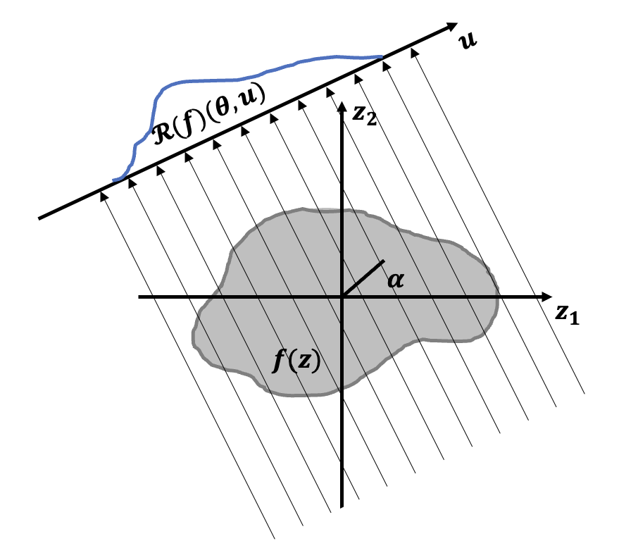
Figure 1: Scheme for the two-dimensional Radon transform. For each unit vector $\theta(\alpha)=({\cos(\alpha),\sin(\alpha))}$, the Radon transform integrates along the line $\langle z,\theta\rangle=u$ for each $u\in\mathbb{R}$.

see Figure 1 for a schematic illustration of the two-dimensional Radon transform. Since $l_{u,\theta}$ and $l_{-u,-\theta}$ are the same line, the Radon transform is an even function that satisfies $\mathcal{R}(f)(\theta,u)=\mathcal{R}(f)(-\theta,-u)$.

The following result shows that the Radon transform of multivariate density functions falls into the space of slicing density functions for each unit vector $\theta$.

Proposition 1.

$\mathcal{R}$ is a valid transform which satisfies assumptions (T0) and (T1).

The inverse Radon transform is related to the Fourier transform. Define the $p$-dimensional Fourier transform $\mathcal{J}_{p}:\,L^{1}(\mathbb{R}^{p})\rightarrow\mathbb{C}$

$$\mathcal{J}_{p}(f)(\iota)=\int_{\mathbb{R}^{p}}e^{-i\langle z,\iota\rangle}f(z)dz,\quad\text{ for all }\iota\in\mathbb{R}^{p},$$

with the one-dimensional Fourier transform $\mathcal{J}_{1}:\,L^{1}(\mathbb{R})\rightarrow\mathbb{C}$ given by $\mathcal{J}_{1}(g)(r)=\int_{\mathbb{R}}g(u)e^{-iur}du$ for all $r\in\mathbb{R}.$ The connection between the Fourier transform and the Radon transform is as follows.

Proposition 2 (Central Slicing Theorem (Bracewell, 1956)).

Assume $f\in\mathcal{F}$. For any real number $r$ and a unit vector $\theta\in\Theta$, $\mathcal{J}_{1}\left({\mathcal{R}(f)}(\theta)\right)(r)=\mathcal{J}_{p}(f)(r\theta).$

The inverse Radon transform has been well investigated both theoretically and numerically (Abeida et al., 2012; Herman, 2009; Mersereau and Oppenheim, 1974). The most commonly used way to reconstruct the original multivariate function from its Radon transform is through the filtered back-projection $\mathcal{R}^{-1}$

$$\mathcal{R}^{-1}\left(\lambda\right)(z)=\frac{1}{2(2\pi)^{p}}\int_{\Theta}\int_{\mathbb{R}}\mathcal{J}_{1}\left({\lambda}(\theta)\right)(r)e^{ir\langle\theta,z\rangle}|r|^{p-1}drd\theta,$$ (3)

which satisfies ${\mathcal{R}^{-1}\left(\mathcal{R}(f)\right)=f}$ for any $f\in\mathcal{F}$ (Natterer, 2001; Epstein, 2007). The inversion formula can be decomposed into two steps. The first step acts as a high-pass filter, suppressing low-frequency components and amplifying high-frequency components. The second step is an angular integral which can be interpreted as a back-projection of the filtered Radon transform (Epstein, 2007; Helgason, 2010). However, $\mathcal{R}^{-1}$ is not a continuous map, and small errors in the reconstruction of $\mathcal{R}(f)$ are amplified (Epstein, 2007). Therefore, regularization is usually applied when reconstructing the original function from its Radon transform (Horbelt et al., 2002; Qureshi et al., 2005; Shepp and Vardi, 1982), often through the use of a ramp filter that has a cut-off in the high-frequency domain (Epstein, 2007; Kak and Slaney, 2001).

Defining the regularizing function $\phi_{\tau}(r)$ with tuning parameter $\tau$ as

$$\phi_{\tau}(r)=\left\{\begin{array}[]{l}1\text{ for }|r|\leq\tau,\\ 0\text{ for }|r|>\tau,\end{array}\right.$$

the regularised inverse map $\check{\mathcal{R}}^{-1}_{\tau}:\Lambda_{\Theta}\rightarrow L^{1}(\mathbb{R}^{p})$ is obtained by cutting off the high-frequency components in the filtered back-projection (3) through

$$\check{\mathcal{R}}_{\tau}^{-1}\left(\lambda\right)(z)=\frac{1}{2(2\pi)^{p}}\int_{\Theta}\int_{\mathbb{R}}\mathcal{J}_{1}\left({\lambda}(\theta)\right)(r)e^{ir\langle\theta,z\rangle}|r|^{p-1}\phi_{\tau}(r)drd\theta.$$ (4)

As this regularized inverse is not guaranteed to be a multivariate density function, normalization is applied to map the resulting $L^{1}$ function into the multivariate density space $\mathcal{F}$ via

$$\mathcal{R}_{\tau}^{-1}\left(\lambda\right)(z)=\begin{cases}\left|\check{\mathcal{R}}_{\tau}^{-1}(\lambda)(z)\right|/\int_{D}\left|\check{\mathcal{R}}_{\tau}^{-1}(\lambda)(z)\right|dz&\text{if}\int_{D}\left|\check{\mathcal{R}}_{\tau}^{-1}(\lambda)(z)\right|dz>0,\\ 1/|D|&\text{otherwise}.\end{cases}$$ (5)

Here $|D|$ represents the Lebesgue measure of the domain set $D$. Note that $\mathcal{R}_{\tau}^{-1}\left(\lambda\right)(z)$ satisfies (F2) while (F1) can be enforced by projecting to the space $\mathscr{F}$ where (F1), (F2) are satisfied.

In practical applications, using a regularized inverse can aid in controlling errors. If $\mathcal{R}(f)$ is approximated by $\widetilde{\mathcal{R}(f)}$, the reconstruction function $\widetilde{f}_{\tau}=\mathcal{R}^{-1}_{\tau}\circ\widetilde{\mathcal{R}(f)}$ will approximate the original function $f$ with the reconstruction error represented as the sum of two error terms

$$\Delta_{\tau}=f-\widetilde{f}_{\tau}=\left(f-\mathcal{R}_{\tau}^{-1}\circ\mathcal{R}(f)\right)+\mathcal{R}_{\tau}^{-1}\circ\left(\mathcal{R}(f)-\widetilde{\mathcal{R}(f)}\right).$$

Let $\Delta_{\tau,1}=f-\mathcal{R}_{\tau}^{-1}\circ\mathcal{R}(f)$ and $\Delta_{\tau,2}=\mathcal{R}_{\tau}^{-1}\circ\left(\mathcal{R}(f)-\widetilde{\mathcal{R}(f)}\right)$.

Theorem 1.

Assume (D1), (F1) and (F2). If $f\in\mathcal{F}$, as $d_{2}(\widetilde{\mathcal{R}(f)},\mathcal{R}(f))\rightarrow 0$ and $\tau\rightarrow\infty$

$$\|\Delta_{\tau,1}\|_{\infty}=O\left(\tau^{-(k-p)}\right),\quad\|\Delta_{\tau,2}\|_{\infty}=O\left(\tau^{p}d_{2}\left(\mathcal{R}(f),\widetilde{\mathcal{R}(f)}\right)\right),$$

$$\|\Delta_{\tau}\|_{\infty}=O\left(\tau^{-(k-p)}+\tau^{p}d_{2}\left(\mathcal{R}(f),\widetilde{\mathcal{R}(f)}\right)\right).$$

The first error term $\Delta_{\tau,1}$ arises from the regularised inverse map and decreases with $\tau$. The second error term $\Delta_{\tau,2}$, results from the approximation of $\mathcal{R}(f)$ and increases with $\tau$. The value of the tuning parameter $\tau$ is then ideally chosen to minimize the total error $\Delta_{\tau}$.

Corollary 1.

Assumptions (T2) and (T3) are satisfied for $\mathcal{R}$ with $C_{1}(\tau)=O(\tau^{-(k-p)})$ and $C_{2}(\tau)=O(\tau^{p})$ as $\tau\rightarrow\infty$.

While the focus of this paper is primarily on the Radon transform, there are other transforms that may also be of interest such as the circular Radon transform (Kuchment, 2006) and the generalized Radon transform (Beylkin, 1984; Ehrenpreis, 2003); see Section S.6 in the Supplement.

3 DISTRIBUTION SLICING AND SLICED DISTANCE

As a formal device we use a map $\varphi$ that assigns its density function to any given distribution, while $\varphi^{-1}$ maps a density function to its corresponding distribution. Consider the metric space $(\mathscr{F},d)$, where $\mathscr{F}$ = $\{\mu\in\mathscr{F}$: $\mu$ has a density function $\varphi(\mu)\in\mathcal{F}\}$ and $d$ is a metric on $\mathscr{F}$. Many metrics can be considered, including the Fisher-Rao metric (Dai, 2022; Zhu and Müller, 2023) or the Wasserstein metric (Gibbs and Su, 2002), which is closely connected with the optimal transport problem (Kantorovich, 2006; Villani, 2003). The $L^{2}$-Wasserstein distance between two random distributions is defined as

$$d_{W}^{2}(\mu_{1},\mu_{2})=\inf_{\begin{subarray}{c}\mu\in\mathcal{P}(\mu_{1},\mu_{2}),\\ {(Z_{1},Z_{2})\sim\mu}\end{subarray}}E\left(\|Z_{1}-Z_{2}\|_{2}^{2}\right),\quad\text{ for all }\mu_{1},\mu_{2}\in\mathscr{F},$$

where $Z_{1}$ and $Z_{2}$ are random variables on $\mathbb{R}^{p}$, $\mu_{1}$ and $\mu_{2}$ are random distributions supported on $D$ and $\mathcal{P}(\mu_{1},\mu_{2})$ is the space of joint probability measures on $D\times D$ with marginal distributions $\mu_{1}$ and $\mu_{2}$. Let $\mathscr{G}=\{\nu\in\mathscr{G}:\nu\text{ has a density function }\varphi(\nu)\in\mathcal{G}\}$ be the space of univariate distributions, $G$ be a map that maps univariate distributions to their corresponding quantile function, while $G^{-1}$ maps a quantile function to its corresponding distribution, and $\mathcal{Q}=\{Q\in\mathcal{Q}:\,\,$There exists a univariate density function $\nu\in\mathscr{G}$,   such that $Q=G(\nu)$$\}$ be the space of quantile functions.

The $L^{2}$-Wasserstein distance of the univariate distributions corresponds to the $L^{2}$ distance between their quantile functions,

$$d_{W}^{2}(\nu_{1},\nu_{2})=\int_{0}^{1}\left(G^{-1}(\nu_{1})(s)-G^{-1}(\nu_{2})(s)\right)^{2}ds,\quad\text{ for all }\nu_{1},\nu_{2}\in\mathscr{G}.$$

When the dimension $p$ of the random distribution is more than $1$, i.e., $p\geq 2$, one does not have an analytic form of the Wasserstein distance and the algorithms to obtain it are complex (Rabin et al., 2011; Peyré et al., 2019). The sliced Wasserstein distance (Bonneel et al., 2015) is a computationally more efficient alternative to the standard Wasserstein distance that utilizes the Radon transform. It has become increasingly popular for multivariate distributions due to its attractive topological and statistical properties (Nadjahi et al., 2019, 2020; Kolouri et al., 2016).

Define the quantile slicing space $\Gamma_{\Theta}$ as a family of maps between $\Theta$ and $\mathcal{Q}$ that

$$\Gamma_{\Theta}=\left\{\gamma\in\Gamma_{\Theta}:\Theta\rightarrow\mathcal{Q},\,\int_{\Theta}\int_{[0,1]}\gamma(\theta)(s)^{2}dsd\theta<\infty\right\}.$$

Note that a univariate distribution is characterized by its quantile function. Define the transform $\varrho:\Gamma_{\Theta}\rightarrow\Lambda_{\Theta}$ as $\varrho(\gamma)(\theta)=\varphi\left(G^{-1}(\gamma(\theta))\right),\gamma\in\Gamma_{\Theta}$, which sends an univariate distribution represented by the quantile function $\gamma(\theta)$ to the corresponding density function. Similarly, $\varrho^{-1}$ can be defined through $\varrho^{-1}(\lambda)(\theta)=G\circ\varphi^{-1}(\lambda(\theta)),\,\lambda\in\Lambda_{\Theta}$; see Figure 2 for a schematic illustration. A slicing transform $\psi$ between $\mathcal{F}$ and $\Lambda_{\Theta}$ can be naturally extended to a transform $\widetilde{\psi}$ between $\mathscr{F}$ and $\Gamma_{\Theta}$,

$$\widetilde{\psi}(\mu)=\varrho^{-1}\circ\psi\circ\varphi(\mu),\quad\mu\in\mathscr{F}.$$ (6)

The inverse transform $\widetilde{\psi}^{-1}$ and regularized inverse transform $\widetilde{\psi}_{\tau}^{-1}$ can be extended as

$$\widetilde{\psi}_{\tau}^{-1}(\gamma)=\varphi^{-1}\circ{\psi}_{\tau}^{-1}\circ\varrho(\gamma),\,\gamma\in\Gamma_{\Theta}\text{ and }\widetilde{\psi}^{-1}(\gamma)=\varphi^{-1}\circ\psi^{-1}\circ\varrho(\gamma),\,\gamma\in\widetilde{\psi}(\mathscr{F}).$$ (7)

Note that the space of $\Gamma_{\Theta}$ is closed and convex while the image space $\widetilde{\psi}(\mathscr{F})$ is not necessarily convex. In Section 6, it will be shown that the convexity of the space plays a role in the convergence result.

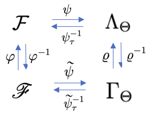
Figure 2: Schematic of maps involved in the slicing transform. Here $\varphi$ maps the multivariate distribution space $\mathscr{F}$ to the multivariate density space $\mathcal{F}$ and $\varrho$ maps the quantile slicing space $\Gamma_{\Theta}$ to the density slicing space $\Lambda_{\Theta}$. A slicing transform $\psi$ and its inverse $\psi_{\tau}^{-1}$ with a tuning parameter $\tau$ between $\mathcal{F}$ and $\Lambda_{\Theta}$ can be naturally extended to a slicing transform between $\mathscr{F}$ and $\Gamma_{\Theta}$ through the induced maps $\widetilde{\psi}$ and $\widetilde{\psi}_{\tau}^{-1}$.

Define the distribution-slicing Wasserstein metric on $\Gamma_{\Theta}$ through the aggregated Wasserstein distance across the slices

$$d_{DW}(\gamma_{1},\gamma_{2}) =\left(\int_{\Theta}d_{W}^{2}\left({G^{-1}}(\gamma_{1}(\theta)),G^{-1}\left(\gamma_{2}(\theta)\right)\right)d\theta\right)^{1/2}$$

$$=\left(\int_{\Theta}\int_{[0,1]}\left(\gamma_{1}(\theta)(s)-\gamma_{2}(\theta)(s)\right)^{2}d\theta\right)^{1/2},\quad\gamma_{1},\gamma_{2}\in\Gamma_{\Theta}.$$ (8)

Here the integral is well defined because of the Cauchy-Schwarz inequality. We then define the slice-averaged Wasserstein distance as

$$d_{SW}(\mu_{1},\mu_{2})=d_{DW}(\widetilde{\psi}(\mu_{1}),\widetilde{\psi}(\mu_{2})),\quad\text{ for all }\mu_{1},\mu_{2}\in\mathscr{F}.$$ (9)

Note that the sliced Wasserstein distance or the generalized sliced Wasserstein distance are special cases of the slice-averaged Wasserstein distance when taking the slicing transform as the Radon or the generalized Radon transform (Bonneel et al., 2015; Kolouri et al., 2019). This distance is well-defined when (T0) holds.

Proposition 3.

The slice-averaged Wasserstein distance is a distance over $\mathscr{F}$ if and only if (T0) is satisfied.

4 SLICED WASSERSTEIN REGRESSION FOR MULTIVARIATE DISTRIBUTIONS

A general approach for the regression of metric-valued responses and Euclidean predictors is Fréchet regression with both global parametric and local smoothing versions (Petersen and Müller, 2019; Chen and Müller, 2022). We provide here a novel extension of Fréchet regression to the case of multivariate distributions by providing two types of sliced regression models. The first model applies Fréchet regression to the multivariate distribution space $\mathscr{F}$ equipped with the slice-averaged Wasserstein distance, while the second model applies a Fréchet regression step for each slice, followed by the regularized inverse transform.

Suppose $(X,\mu)\sim F$ is a random pair, where predictors $X$ and responses $\mu$ take values in $\mathbb{R}^{q}$ and $\mathscr{F}$ and $F$ is their joint distribution. Denote the marginal distributions of $X$ and $\mu$ as $F_{X}$ and $F_{\mu}$ respectively, and assume that mean $E(X)$ and variance $\operatorname*{Var}(X)$ exist, where $\operatorname*{Var}(X)$ is positive definite. The conditional distributions $F_{\mu|X}$ and $F_{X|\mu}$ are also assumed to exist. The Fréchet mean and Fréchet variance of the random distribution $\mu$ are defined as

$$\omega_{\oplus}=\operatorname*{argmin}_{\omega\in\mathscr{F}}E\left[d^{2}(\mu,\omega)\right],\quad V_{\oplus}=E\left[d^{2}(\mu,\omega_{\oplus})\right].$$ (10)

The conditional Fréchet mean, which corresponds to the regression function of $\mu$ given $X=x$, corresponds to an M estimator defined as

$$m(x)=\operatorname*{argmin}_{\omega\in\mathscr{F}}M(\omega,x),\quad M(\cdot,x)=E\left[d^{2}(\mu,\cdot)|X=x\right],$$ (11)

where $M(\cdot,x)$ is referred to as the conditional Fréchet function. The global Fréchet regression given $x$ is defined as

$$m_{G}(x)=\operatorname*{argmin}_{\omega\in\mathscr{F}}M_{G}(\omega,x),\quad M_{G}(\cdot,x)=E\left[s_{G}(X,x)d^{2}(\mu,\cdot)\right],$$ (12)

where the weight $s_{G}(X,x)=1+(X-E(X))^{T}\operatorname*{Var}(X)^{-1}(x-E(X))$ is linear in $x$.

The proposed slice-averaged Wasserstein (SAW) regression employs Fréchet regression over the multivariate distribution space $\mathscr{F}$ equipped with the slice-averaged Wasserstein distance,

$$m^{SAW}(x)=\operatorname*{argmin}_{\omega\in\mathscr{F}}M^{SAW}(\omega,x),\quad M^{SAW}(\cdot,x)=E\left[d_{SW}^{2}(\mu,\cdot)|X=x\right].$$ (13)

The global slice-averaged Wasserstein (GSAW) regression given $x$ is defined as

$$m_{G}^{SAW}(x)=\operatorname*{argmin}_{\omega\in\mathscr{F}}M_{G}^{SAW}(\omega,x),\quad M_{G}^{SAW}(\cdot,x)=E\left[s_{G}(X,x)d_{SW}^{2}(\mu,\cdot)\right].$$ (14)

The second proposed model is the slice-wise Wasserstein (SWW) regression, where Fréchet regression is applied over the quantile slicing space $\Gamma_{\Theta}$, equipped with the distribution-slicing Wasserstein metric, followed by the regularized inverse transform,

$$m^{SWW}_{\tau}(x)=\widetilde{\psi}^{-1}_{\tau}\left[\operatorname*{argmin}_{\gamma\in\Gamma_{\Theta}}M^{SWW}(\gamma,x)\right],\quad M^{SWW}(\cdot,x)=E\left[d_{DW}^{2}(\widetilde{\psi}(\mu),\cdot)|X=x\right].$$ (15)

The global slice-wise Wasserstein (GSWW) regression given $x$ is

$$m_{G,\tau}^{SWW}(x)=\widetilde{\psi}_{\tau}^{-1}\left[\operatorname*{argmin}_{\gamma\in\Gamma_{\Theta}}M_{G}^{SWW}(\gamma,x)\right],\quad M_{G}^{SWW}(\cdot,x)=E\left[s_{G}(X,x)d_{DW}^{2}(\widetilde{\psi}(\mu),\cdot)\right].$$ (16)

We note that for SAW based models the minimization is carried out over the space $\mathscr{F}$ and thus is automatically a multivariate distribution, that provides an implementation of the conditional Fréchet mean, while for SWW based models the minimization is carried out slicewise and since the slicewise minimizers are not guaranteed to be situated in $\psi(\mathscr{F})$, the regularized inverse is required here as the inverse $\psi^{-1}$ is only defined on $\psi(\mathscr{F})$. Formally, we show that SWW regression is equivalent to applying the Fréchet regression along each slice $\theta$ followed by an inverse transform.

Proposition 4.

Let $\gamma_{G,x}=\operatorname*{argmin}_{\gamma\in\Gamma_{\Theta}}M_{G}^{SWW}(\gamma,x)$, see (16). It can be characterized as

$$\gamma_{G,x}(\theta)=\operatorname*{argmin}_{\nu\in\mathscr{G}}E\left[s_{G}(X,x)d_{W}^{2}\left(G^{-1}\left(\widetilde{\psi}(\mu)(\theta)\right),\nu\right)\right],\quad{\text{for almost all }}\theta\in\Theta.$$

This characterization of the SWW regression provides a practical implementation of this method. Proposition S4 in the Supplement further establishes the connection between the SWW and the SAW regression, demonstrating that the search space of SAW is a subset of the search space of SWW. Note that besides global Fréchet regression as described above one can analogously develop more flexible local Fréchet regression based models for SAW and SWW. Details about implementations with local Fréchet regression are in Section S.3 in the Supplement.

5 ESTIMATION

Suppose we have a sample of independent random pairs $\{(X_{i},\mu_{i})\}_{i=1}^{n}\sim F$, then the sample mean and variance can be obtained as

$$\bar{X}=n^{-1}\sum_{i=1}^{n}X_{i},\quad\hat{\Sigma}=n^{-1}\sum_{i=1}^{n}(X_{i}-\bar{X})(X_{i}-\bar{X})^{T}.$$

If random distributions $\mu_{i}$ are fully observed, sample estimators of the GSAW and GSWW are

$$\check{m}_{G}^{SAW}(x)=\operatorname*{argmin}_{\omega\in\mathscr{F}}\check{M}_{G}^{SAW}(\omega,x),\quad\check{M}_{G}^{SAW}(\cdot,x)=n^{-1}\sum_{i=1}^{n}\left[s_{iG}(x)d_{SW}^{2}(\mu_{i},\cdot)\right],$$

$$\check{m}_{G,\tau}^{SWW}(x)=\widetilde{\psi}_{\tau}^{-1}\left[\operatorname*{argmin}_{\gamma\in\Gamma_{\Theta}}\check{M}_{G}^{SWW}(\gamma,x)\right],\quad\check{M}_{G}^{SWW}(\cdot,x)=n^{-1}\sum_{i=1}^{n}\left[s_{iG}(x)d_{DW}^{2}(\widetilde{\psi}(\mu_{i}),\cdot)\right],$$

where $s_{iG}(x)=1+(X_{i}-\bar{X})^{T}\hat{\Sigma}^{-1}(x-\bar{X})$ is the sample version estimator of $s_{G}(X,x)$. In practice, random distributions $\{\mu_{i}\}_{i=1}^{n}$ may not be fully observed and one may have only observations that they generate. In such scenarios, a preliminary density estimation step may be required; further details on this are in Section S.2 in the Supplement. If the random distributions $\mu_{i}$ are estimated by the product kernel density estimator $\hat{\mu}_{i}$ through (S.1), the corresponding estimators are

$$\hat{m}_{G}^{SAW}(x)=\operatorname*{argmin}_{\omega\in\mathscr{F}}\hat{M}_{G}^{SAW}(\omega,x),\quad\hat{M}_{G}^{SAW}(\cdot,x)=n^{-1}\sum_{i=1}^{n}\left[s_{iG}(x)d_{SW}^{2}\left(\hat{\mu}_{i},\cdot\right)\right],$$ (17)

$$\hat{m}_{G,\tau}^{SWW}(x)=\widetilde{\psi}_{\tau}^{-1}\left[\operatorname*{argmin}_{\gamma\in\Gamma_{\Theta}}\hat{M}_{G}^{SWW}(\gamma,x)\right],\quad\hat{M}_{G}^{SWW}(\cdot,x)=n^{-1}\sum_{i=1}^{n}\left[s_{iG}(x)d_{DW}^{2}(\widetilde{\psi}(\hat{\mu}_{i}),\cdot)\right].$$ (18)

Sample version estimators of the local smoothing models for SAW and SWW, along with an analysis of the bandwidth selection, can be found in Section S.3.2 in the Supplement.

A practical data-driven approach to select the tuning parameter $\tau$ when an i.i.d. sample of random pairs $\{(X_{i},\mu_{i})\}_{i=1}^{n}$ is available can be obtained by leave-one-out cross-validation. Specifically, we aim to minimize the discrepancy between predicted and observed distributions, given by

$$\hat{\tau}=\operatorname*{argmin}_{\tau}\sum_{i=1}^{n}d_{SW}^{2}({\mu_{i}},\hat{m}_{G,\tau,-i}^{SWW}(X_{i})),$$

where $\hat{m}_{G,\tau,-i}^{SWW}(X_{i})$ is the prediction at $X_{i}$ from the GSWW regression of the $i$th-left-out sample $\{(X_{i^{{}^{\prime}}},\mu_{i^{{}^{\prime}}})\}_{i^{{}^{\prime}}\neq i}$. When the sample size $n$ exceeds $30$, we substitute leave-one-out cross-validation with 5-fold cross-validation to strike a balance between computational efficiency and the accuracy of the tuning parameter selection.

We define a slice-averaged Wasserstein $R^{2}$ coefficient to quantify the discrepancy between observed distributions and predicted distributions from the regression model as

$$R_{\oplus}^{2}=1-\frac{E[d_{SW}^{2}(\mu,m(x))]}{E[d_{SW}^{2}(\mu,\mu_{\oplus})]},$$

where $m(x)$ is a regression object through either SAW or SWW regression and $\mu_{\oplus}$ is the slice-averaged Wasserstein Fréchet mean $\mu_{\oplus}=\operatorname*{argmin}_{\omega\in\mathscr{F}}d_{SW}^{2}(\mu,\omega)$.

One can estimate $R_{\oplus}^{2}$ from a sample $\{(X_{i},\mu_{i})\}_{i=1}^{n}$ by

$$\hat{R}_{\oplus}^{2}=1-\frac{\sum_{i=1}^{n}d_{SW}^{2}({\mu}_{i},\hat{m}(x))}{\sum_{i=1}^{n}d_{SW}^{2}({\mu}_{i},\hat{\mu}_{\oplus})},$$ (19)

where $\hat{\mu}_{\oplus}=\operatorname*{argmin}_{\omega\in\mathscr{F}}n^{-1}\sum_{i=1}^{n}d_{SW}^{2}({\mu}_{i},\omega)$ is the sample Fréchet mean and $\hat{m}(x)$ is the sample estimator of the regression object $m(x)$ through either SAW or SWW regression.

6 ASYMPTOTIC CONVERGENCE

The study of convergence of the SAW regression and the SWW regression requires a curvature condition at the true minimizer, as commonly required for M estimators. The Fréchet regression requires such a curvature condition which has been established for the case of univariate distributions but not for multivariate distributions as objects. Certain convexity assumptions (Fan and Müller, 2021; Boissard et al., 2011) have been typically required previously. To establish asymptotic convergence, we require the following assumptions.

(P1) $N(n)=\min_{1\leq i\leq n}N_{i}\gtrsim n^{(p+4)/8}$, where $N_{i}$ is the number of random observations for the $i$-th distribution $\mu_{i}$ when densities need to be estimated (Section S.2 in the Supplement).
(P2) $\operatorname*{argmin}_{\gamma\in\Gamma_{\Theta}}M_{G}^{SWW}(\gamma,x)$ as per (16) is in $\widetilde{\psi}(\mathscr{F})$.
(A1) $\widetilde{\psi}(\mathscr{F})$ is closed and convex.

Assumption (P1) is used to establish that the convergence rate of the multivariate density estimated from random observations is faster than the parametric rate $n^{-1/2}$, as shown in (S.2). Assumption (P2) ensures the underlying minimizer of the GSWW regression belongs to the image space of the slicing transform. Assumption (A1) guarantees the existence and uniqueness of the minimizer of the SAW regression. Additional assumptions (K1) and (K2) in Section S.1 in the Supplement are standard for the kernel density estimation.

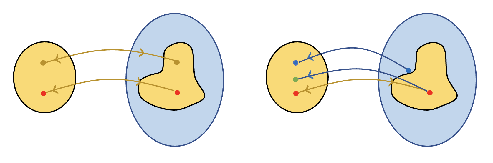
Figure 3: Diagram for SAW (left) and SWW (right) sample estimation. The red dots are population minimizers, the yellow dots are the sample SAW minimizer, the blue dots are the sample SWW minimizers and the green dot is the intermediate state used to facilitate the error analysis of SWW. Bidirectional yellow curves correspond to $\widetilde{\psi}$ and $\widetilde{\psi}^{-1}$ while directional blue curves are connected with the regularized inverse $\widetilde{\psi}_{\tau}^{-1}$.

Theorem 2.

Assume (D1), (F1), (F2), (K1), (K2), (P1), (A1) and (T0)-(T2). For a fixed $x\in\mathbb{R}^{q}$, it holds that for $m_{G}^{SAW}(x)$ and $\hat{m}_{G}^{SAW}(x)$ as per (14) and (17),

$$d_{SW}\left(m_{G}^{SAW}(x),\hat{m}_{G}^{SAW}(x)\right)=O_{p}(n^{-1/2}).$$

Furthermore, for a given $B>0$ and any $\epsilon>0$,

$$\sup_{\|x\|_{E}\leq B}d_{SW}\left(m_{G}^{SAW}(x),\hat{m}_{G}^{SAW}(x)\right)=O_{p}(n^{-1/(2+\epsilon)}).$$

Under regularity conditions, using the global estimator for tracking the global SAW target thus yields a parametric convergence rate that does not depend on the dimension of the distribution space. For SAW, convergence in terms of the sup norm is not possible due to the inverse transform $\widetilde{\psi}^{-1}$, which amplifies estimation error in the image space, as exemplified above for the Radon transform. However, for SWW, the regularized inverse transform $\widetilde{\psi}_{\tau}^{-1}$ is continuous due to (T3), and thus one can obtain sup norm convergence. Under assumption (P2), we define the population-level target $m_{G}^{SWW}$ by

$$m_{G}^{SWW}=\widetilde{\psi}^{-1}\left[\operatorname*{argmin}_{\gamma\in\Gamma_{\Theta}}M_{G}^{SWW}(\gamma,x)\right],$$ (20)

where $M_{G}^{SWW}$ is defined as per (16).

Theorem 3.

Assume (D1), (D2), (F1), (F2), (G1), (G2), (K1), (K2), (P1), (P2), (T0)-(T3). For a fixed $x\in\mathbb{R}^{q}$, it holds that for $m_{G}^{SWW}(x)$ and $\hat{m}_{G,\tau}^{SWW}(x)$ as per (20) and (18), $C_{1}(\tau)$ and $C_{2}(\tau)$ from (T3),

$$d_{\infty}\left(m_{G}^{SWW}(x),\hat{m}_{G,\tau}^{SWW}(x)\right)=O_{p}\left({C_{1}(\tau)+C_{2}(\tau)}{n^{-2/7}}\right).$$

Furthermore, for a given $B>0$ and any $\epsilon>0$,

$$\sup_{\|x\|_{E}\leq B}d_{\infty}\left(m_{G}^{SWW}(x),\hat{m}_{G,\tau}^{SWW}(x)\right)=O_{p}\left(C_{1}(\tau)+C_{2}(\tau)n^{-2/(7+\epsilon)}\right).$$

The reconstruction error has two parts. The first term $C_{1}(\tau)$ is linked to the approximation bias in the reconstruction, while the second term $C_{2}(\tau)$ ensures that the approximation in the transformed space $\Gamma_{\Theta}$ is not excessively amplified. See Figure 3. Additionally, since we estimate the derivative of the quantile function to reconstruct the multivariate density, an extra cost is incurred. In the case of the Radon transform, Corollary 2 shows that the curse of dimensionality is manifested in both $C_{1}(\tau)$ and $C_{2}(\tau)$, as a higher order of smoothness is required for a higher dimensional distribution to achieve the same convergence rate.

Corollary 2.

When taking the Radon transform $\mathcal{R}$ and the corresponding regularized inverse $\mathcal{R}^{-1}_{\tau}$ as per (2) and (5), under assumptions of Theorem 3,

$$d_{\infty}\left(m_{G}^{SWW}(x),\hat{m}_{G,\tau}^{SWW}(x)\right)=O_{p}\left(\tau^{-(k-p)}+\tau^{p}{n^{-2/7}}\right),$$

$$\sup_{\|x\|_{E}\leq B}d_{\infty}\left(m_{G}^{SWW}(x),\hat{m}_{G,\tau}^{SWW}(x)\right)=O_{p}\left(\tau^{-(k-p)}+\tau^{p}n^{-2/(7+\epsilon)}\right),$$

and with $\tau\sim n^{1/3k}$,

$$d_{\infty}\left(m_{G}^{SWW}(x),\hat{m}_{G,\tau}^{SWW}(x)\right)=O_{p}\left(n^{-2(k-p)/7k}\right).$$

$$\sup_{\|x\|_{E}\leq B}d_{\infty}\left(m_{G}^{SWW}(x),\hat{m}_{G,\tau}^{SWW}(x)\right)=O_{p}\left(n^{-2(k-p)/(7k+\epsilon)}\right).$$

For the local version of the SAW and SWW regression, the analogous results are provided in Section S.3.3 in the Supplement.

7 NUMERICAL ALGORITHM

7.1 SAW Regression

To solve problem (17) in practice, we use a numerical optimization process proposed in Bonneel et al. (2015) that involves parametrizing a probability measure with equal weights. Specifically, we use random observations $\mathbf{W}=\{\mathbf{W}_{j}\}_{j=1}^{N}\in\mathbb{R}^{p\times N}$ where each observation ${\mathbf{W}}_{j}\in\mathbb{R}^{p}$ follows a distribution characterized by a density function $f_{\mathbf{W}}$ in $\mathcal{F}$. We introduce the Radon slicing operation $\langle\cdot,\theta\rangle:\mathbb{R}^{p}\rightarrow\mathbb{R}$ for each random observation, resulting in a univariate distribution with the density function $\mathcal{R}\circ f_{\mathbf{W}}(\theta)$. The multivariate distribution $\mu$ corresponding to the density $f_{\mathbf{W}}$ can be represented as a discrete input measure $\mu_{\mathbf{W}}=\frac{1}{N}\sum_{j=1}^{N}\delta_{\mathbf{W}_{j}}$. Similarly, we represent the $i$-th distribution $\mu_{i}$ as a discrete input measure $\mu_{\mathbf{W}^{(i)}}=\frac{1}{N}\sum_{j=1}^{N}\delta_{\mathbf{W}_{ij}}$ where $\mathbf{W}^{(i)}=\{\mathbf{W}_{ij}\}_{j=1}^{n_{i}}\in\mathbb{R}^{p\times N}$ and $\mathbf{W}_{ij}\sim\mu_{i}$. The GSAW regression of (17) given $X=x$ can be represented as

$$\operatorname*{argmin}_{\mathbf{W}\in\mathbb{R}^{p\times N}}\mathcal{M}_{G}(\mathbf{W},x)=n^{-1}\sum_{i=1}^{n}\left[s_{iG}(x)d_{SW}^{2}(\mu_{\mathbf{W}^{(i)}},\mu_{\mathbf{W}})\right].$$ (21)

The following proposition states that the target function is smooth for the Radon transform. Denote $\mathbf{W}(\theta)=(\langle\mathbf{W}_{j},\theta\rangle)_{j=1}^{N}\in\mathbb{R}^{N}$ and similarly $\mathbf{W}^{(i)}(\theta)=(\langle\mathbf{W}_{ij},\theta\rangle)_{j=1}^{N}\in\mathbb{R}^{N}$. For any $A=\{A_{j}\}_{j=1}^{N}\in\mathbb{R}^{N}$ where $A_{j}\in\mathbb{R}$, $\Pi_{A}$ is a permutation operator on $A$, such that $\Pi_{A}(A)=(A_{\Pi(1)},A_{\Pi(2)},...,A_{\Pi(N)})^{T}$ with $A_{\Pi(1)}\leq A_{\Pi(2)}\leq\cdots\leq A_{\Pi(N)}$.

Proposition 5 (Theorem 1 (Bonneel et al., 2015)).

For each fixed $x$ and $N_{i}\equiv N$, $\mathcal{M}_{G}(\mathbf{W},x):\mathbb{R}^{p\times N}\rightarrow\mathbb{R}$ is a $L^{1}$ function with a uniformly $\rho_{G}$-Lipschitz gradient for some $\rho_{G}>0$ given by

$$\nabla\mathcal{M}_{G}(\mathbf{W},x)=n^{-1}\sum_{i=1}^{n}\left[s_{iG}(x)\int_{\Theta}\theta\left(\mathbf{W}(\theta)-\Pi_{\mathbf{W}(\theta)}^{-1}\circ\Pi_{\mathbf{W}^{(i)}(\theta)}\circ\mathbf{W}^{(i)}(\theta)\right)^{T}d\theta\right].$$

The operation $\Pi_{\mathbf{W}(\theta)}^{-1}\circ\Pi_{\mathbf{W}^{(i)}(\theta)}\circ\mathbf{W}^{(i)}(\theta)$ aligns $\mathbf{W}^{(i)}(\theta)$ with $\mathbf{W}(\theta)$ in the sense of non-decreasing order for calculating the empirical Wasserstein distance. In practice, an equidistant grid $(\theta_{1},\theta_{2},...,\theta_{L})$ along the angular coordinate of the polar coordinate system is used to approximate the integration along $\Theta$. Note that (21) is non-convex and Algorithm 1 uses gradient descent to find a stationary point. See Section S.3.4 in the Supplement for further discussion about the local model for SAW.

Algorithm 1 GSAW Algorithm when using the Radon Transform

1:Initialize a grid $(\theta_{1},\theta_{2},...,\theta_{L})$ along $\Theta$

2:Set $N=\min_{i=1,...,n}N_{i}$, threshold $\varepsilon$ and step $\eta$

3:For each $\mu_{\mathbf{W}^{(i)}}$, downsample $\mathbf{W}^{(i)}$ such that $\mathbf{W}^{(i)}\in\mathbb{R}^{p\times N}$

4:Initialize $\mathbf{W}^{[0]}\in\mathbb{R}^{p\times N}$ arbitrarily and fix the output predictor $X=x$

5:repeat

6:     Calculate $\nabla\mathcal{M}_{G}(\mathbf{W}^{[k]},x)$

$$\nabla\mathcal{M}_{G}(\mathbf{W}^{[k]},x)=(nL)^{-1}\sum_{i=1}^{n}\sum_{l=1}^{L}s_{iG}(x)\theta_{l}\left(\mathbf{W}(\theta_{l})-\Pi_{\mathbf{W}(\theta_{l})}^{-1}\circ\Pi_{\mathbf{W}^{(i)}(\theta_{l})}\circ\mathbf{W}^{(i)}(\theta_{l})\right)^{T}$$

7:     $\mathbf{W}^{[k+1]}=\mathbf{W}^{[k]}-\eta\nabla\mathcal{M}_{G}(\mathbf{W}^{[k]},x)$

8:until Algorithm converge $\left\|\mathbf{W}^{[k+1]}-\mathbf{W}^{[k]}\right\|_{2}/\left\|\mathbf{W}^{[k]}\right\|_{2}<\varepsilon$

7.2 Slicewise Wasserstein Regression

Since the SWW regressions are conducted slicewise and therefore do not entangle with each other, we can leverage parallel computing to significantly enhance the computing efficiency and do not require the permutation operator. Note that the local model for SWW can be implemented analogously simply by using local instead of global Fréchet regression in the algorithm.

Algorithm 2 GSWW Algorithm for the Radon Transform

1:Initialize a grid $(\theta_{1},\theta_{2},...,\theta_{L})$ along $\Theta$ and fix the output predictor $X=x$

2:Perform a Radon slicing operation over random observations, i.e. $\langle\mathbf{W}^{(i)},\theta_{l}\rangle$, $i=1,...,n,l=1,...,L$

3:for $l=1,...,L$ do in parallel

4:     Apply the Fréchet regression for sliced random pairs, $\left(X_{i},\langle\mathbf{W}^{(i)},\theta_{l}\rangle\right)$, $i=1,...,n$

5:     Calculate the fitted density on the output $X=x$ as $\hat{\lambda}(\theta_{l})$

6:end for

7:Apply the regularized Radon reconstruction $\hat{f}=\mathcal{R}_{\tau}^{-1}(\hat{\lambda})$ through (5)

8 SIMULATION STUDY

We consider two simulation scenarios, one of which is inspired by Fan and Müller (2021) and involves bivariate Gaussian distributions with mean and covariance depending linearly on a predictor variable $x\in[-0.5,0.5]$, with distributions truncated on the compact support $[-1,1]\times[-1,1]$. We generate a scaler predictor $X$ from a uniform distribution on $[-0.5,0.5]$ and the distributional trajectories as $\alpha|X=x\sim\mathcal{N}((0.4x,0.4x)^{T},\mathcal{V}(x))$ where $\mathcal{V}(x)=V\mathscr{D}V^{T}$ with $V=\left[\begin{array}[]{cc}\frac{\sqrt{2}}{2}&\frac{\sqrt{2}}{2}\\ -\frac{\sqrt{2}}{2}&\frac{\sqrt{2}}{2}\end{array}\right]$, $\mathscr{D}=\text{diag}(\xi_{1},\xi_{2})$ with $(\xi_{1},\xi_{2})|X=x\sim\frac{1}{100}\mathcal{N}\left((1.25+0.5x,0.75-0.5x)^{\prime},0.01\mathbf{I}_{2}\right)$.

The second simulation scenario features distributional trajectories $\alpha|X=x\sim\mathcal{N}(0.4x,0.4x-0.05\sin(\pi x/0.5))^{T},\mathcal{V}(x))$ with the same covariance matrix $\mathcal{V}(x)$ as above and $(\xi_{1},\xi_{2})|X=x\sim\frac{1}{100}\mathcal{N}((0.75+x^{2},0.625+x^{3})^{\prime},0.01\mathbf{I}_{2})$.

We perform simulations with sample sizes $n=50$ and $n=100$, each with two sets of random observations, $N=50$ and $N=100$. The mean integrated sliced Wasserstein error (MISWE) is used as the evaluation metric, $\text{MISWE}={E\left[\int_{0}^{1}d_{SW}^{2}(\hat{m}(x),m(x))dx\right]}$, where $\hat{m}(x)$ is the fitted and $m(x)$ the true model. The empirical MISWE is estimated through Monte Carlo runs,

$$\text{EMISWE}=\frac{1}{M_{c}}\sum_{k=1}^{M_{c}}\int_{0}^{1}d_{SW}^{2}(\hat{m}_{k}(x),m(x))dx,$$ (22)

where $\hat{m}_{k}(x)$ is the fit for the $k$-th Monte Carlo run. Results are presented in Table 1.

		$n=50$			$n=100$
Set	Methods	$N=50$	$N=100$		$N=50$	$N=100$
Set1	GSWW	7.84	7.36		6.92	6.80
	GSAW	13.2	11.0		12.0	10.8
Set2	GSWW	10.5	9.70		9.80	9.52
	GSAW	13.4	11.9		13.1	11.7

Table 1: Simulation results for Set1 and Set2. The EMISWE as per (22) are reported for different sample sizes of distributions ($n$) and numbers of random observations ($N$). The results are averaged over 100 Monte Carlo runs and reported in units of $10^{-4}$.

In the first set, both the GSAW and GSWW methods align with the true model, resulting in a smaller error than local models. In the second set, the local models retrieve the nonlinear true model, leading to a smaller error than the global models. Across both settings, both the global and local SWW methods consistently demonstrate superior performance compared to their SAW method counterparts. See Section S.4 in the Supplement for additional simulation results for local models. This can be attributed to the fact that the SWW method seeks to identify a unique minimizer for each slice where the objective function is guaranteed to be convex. Moreover, by aggregating the slicing information, the regularized inverse ensures that the overall error is kept under control. On the other hand, the SAW method employs gradient descent to directly search for a multivariate distribution target and requires a convexity assumption.

9 DATA ANALYSIS

In this section, we present two data analyses by using global models of the sliced Wasserstein regression on blood pressure and mortality data. In Section S.5 of the Supplement, we employ the local models of sliced Wasserstein regression to analyze the Exchange Traded Funds data.

9.1 Baltimore Longitudinal Study of Aging

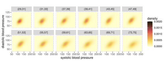
Figure 4: Observed smoothed densities for some selected age groups.

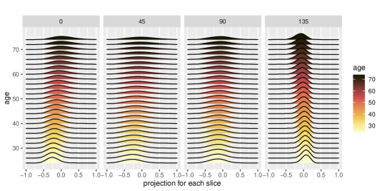
Figure 5: Fréchet regressions for GSWW between age (predictor, on the $y$-axis) and fitted slicing distributions (responses, on the $x$-axis) for various projections. The number at the top of each panel indicates the angle of the respective projection with the $x$-axis (SBP) in Figure 4.

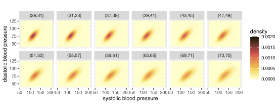
Figure 6: Fitted density surfaces for some age groups obtained by the GSWW version of sliced Wasserstein regression with sliced Wasserstein fraction of variance explained at level 0.80.

Figure 7: Fitted density surfaces for some age groups obtained by the GSAW version of sliced Wasserstein regression with sliced Wasserstein fraction of variance explained at level 0.75.

Systolic (SBP) and diastolic (DBP) blood pressure were assessed longitudinally in the Baltimore longitudinal study of aging (BLSA) https://www.blsa.nih.gov/, where 16715 measurements are available from approximately 2800 individuals. The number of visits per individual ranged from 1 to 26, and the ages of the participants from 17 to 75 years.

We divided the data into 25 groups, each containing over 200 randomly sampled measurements and used 51 equidistant grid points in each direction over the domains $[75,225]$ for SBP and $[40,125]$ for DBP. Figure 4 shows estimated kernel density surfaces for randomly selected age groups, which correspond to the observed response distributions, while Figure 5 illustrates global Fréchet regressions for representative angles of GSWW regression. Our analysis reveals that as age increases, the center of the slicing distribution shifts towards higher values for 0, 45, and 90-degree angles relative to the $x$ axis (SBP), and towards lower values at a 135-degree angle. This indicates that the increase along SBP is faster compared to DBP as people age. Moreover, variation is seen to increase with age for all slices.

Figures 6 and 7 present the fitted density surfaces using GSWW and GSAW regression models, respectively. The sliced Wasserstein fraction of variance explained for GSWW and GSAW models, as per (19), is 0.80 and 0.75, respectively. Our analysis reveals that both models capture the underlying transition from a safe region centered at around SBP = 110, DBP = 75 to an unsafe region centered at around SBP = 135, DBP = 90 with higher age. Additionally, there is an increase of covariance with age. It also emerges that the GSWW approach provides better fits than GSAW, providing further support for the slice-wise optimization approach of SWW.

9.2 Excess Winter Deaths in Europe

Excess winter deaths are a social and health challenge. For European countries they have become an acute problem due to rapidly rising heating costs. It is known that in general Northern European countries have lower excess winter mortality rates compared to Southern European countries (Healy, 2003; Fowler et al., 2015). Our goal in this analysis was to follow up on this by modeling conditional distributions directly, rather than characterizing mortality effects through summary statistics such as sample mean or standard deviation, as was done in previous studies.

We focused on $n=31$ countries with available data from 1999 to 2021, for which we adopted the proposed GSWW and GSAW models with the country-level base winter temperature averaged from 1961-90 as predictor and the country-level bivariate distribution between the excess rate of winter mortality relative to the previous summer and winter temperature anomaly relative to the base winter temperature from 1961-90 as the response. The absolute numbers of deaths in each of the 31 European countries from 1999 to 2021 were obtained from the Eurostat database https://ec.europa.eu/eurostat/web/main/data/database and the average winter temperature anomalies and the base winter temperatures from 1961-90 from https://www.uea.ac.uk/groups-and-centres/climatic-research-unit/data.

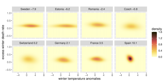
Figure 8: Observed smoothed densities of the joint distributions of excess winter death rates ($y$-axis) and winter temperature anomaly ($x$-axis) for a few European countries, arranged in order of their base winter temperature. Each panel is labeled by the name of the country; the corresponding average base winter temperature (in degrees C) from 1961-1990 is also indicated.

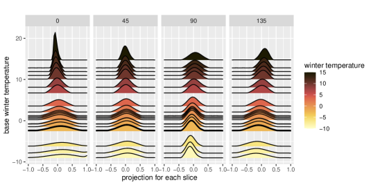
Figure 9: Fréchet regression between the base winter temperature (predictor, on the $y$-axis) and the slicing distributions (responses, on the $x$-axis) for various projections. The number at the top of each panel indicates the angle of the respective projection with the $x$-axis in Figure 8.

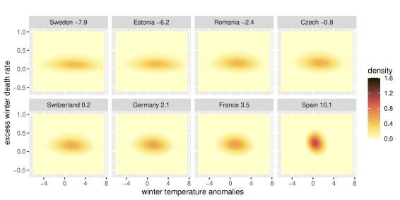
Figure 10: Fitted density surfaces for randomly selected countries obtained by the GSWW version of sliced Wasserstein regression with sliced Wasserstien fraction of variance explained at level 0.53.

The observed smoothed bivariate distributions are in Figure 8 for a few selected countries, ordered by the base winter temperature. Figure 9 displays the global Fréchet regression for some representative projections and illustrates the Fréchet regression step of the GSWW sliced Wasserstein regression. As the base temperature increases, the variance of the temperature anomalies decreases and the excess winter death rates shift to a higher level. Additionally, from the slicing angle at 135 degrees, the excess death rate becomes more responsive to temperature anomalies as the base winter temperature increases, as exemplified by Spain.

The fitted densities obtained from the GSWW model are shown in Figure 10 with the corresponding sliced Wasserstein fraction of variance explained taking a value of 0.53; the fitted densities when fitting GSAW for the same countries can be found in Section S.10 in the Supplement. Countries with warmer climates typically experience a higher rate of excess deaths during the winter season compared to colder countries for the same temperature anomaly. For instance, in Spain, a country with a warm climate, there is a roughly 30% increase in the number of deaths during the winter months compared to the preceding summer. However, in Sweden, a country with a colder climate, this increase is only around 15%. Again, the fitted density for Spain is illustrative for this effect.

Supplement to "Sliced Wasserstein Regression"

S.1 ADDITIONAL ASSUMPTIONS

(K1) The kernel function $\kappa$ as per (S.1) is nonnegative, has bounded support and is symmetric around 0.

(K2) $\int\kappa(u)^{2}du<\infty$ and $\int u^{2}\kappa(u)du<\infty$.

(P3) $\operatorname*{argmin}_{\gamma\in\Gamma_{\Theta}}M_{L,h}^{SWW}(\gamma,x)\in\widetilde{\psi}(\mathscr{F})$ as per (S.5).
(L1) The kernel $K$ used for the local sliced Wasserstein regression in Section S.3 is a probability density function and is symmetric around zero. Furthermore, defining $K_{kj}=\int_{\mathbb{R}}K^{k}(u)u^{j}du$, $|K_{14}|$ and $|K_{26}|$ are both finite.
(L2) The marginal density of $X,$ as well as the conditional density of $X$ given $\mu=\omega$, $\mathcal{E}_{X|\mu}(\cdot,\omega)$, exist and are twice continuously differentiable, the latter for all $\omega\in\mathscr{F}$, and $\sup_{x,\omega}|\left(\partial^{2}\mathcal{E}_{X|\mu}/\partial x^{2}\right)(x,\omega)|<\infty$. Additionally, for any open $U\subset\mathscr{F}$, $\int_{U}dF_{\mu|X}(x,\omega)$ is continuous as a function of $x$.
(L3) The kernel $K$ is a probability density function, symmetric around zero, and uniformly continuous on $\mathbb{R}$. Furthermore, defining $K_{jk}=\int_{\mathbb{R}}K(u)^{j}u^{k}du$, for $j,k\in\mathbb{N}$, $|K_{14}|$ and $|K_{26}|$ are both finite. The derivative $K^{\prime}$ exists and is bounded on the support of $K$, i.e., $\sup_{K(u)>0}|K^{\prime}(u)|<\infty$; additionally, $\int_{\mathbb{R}}u^{2}|K^{\prime}(u)|(|u\log|u||)^{1/2}du<\infty$.
(L4) Let $\mathcal{T}$ be a closed interval in $\mathbb{R}$ and $\mathcal{T}^{o}$ be its interior. The marginal density of $X$, $\mathcal{E}_{X}(x)$, as well as the conditional density of $X$ given $\mu=\omega$, $\mathcal{E}_{X|\mu}(\cdot,\omega)$, exist and are twice continuously differentiable on $\mathcal{T}^{o}$, the latter for all $\omega\in\mathscr{F}$. The marginal density $\mathcal{E}_{X}(x)$ is bounded away from zero on $\mathcal{T}$, $\inf_{x\in\mathcal{T}}\mathcal{E}_{X}(x)>0$. The second-order derivative $\mathcal{E}_{X}^{\prime\prime}(x)$ is bounded, $\sup_{x\in\mathcal{T}^{o}}|\mathcal{E}_{X}^{\prime\prime}(x)|<\infty$. The second-order partial derivatives $(\partial^{2}\mathcal{E}_{X|\mu}(x,\omega)/\partial x^{2})(x,\omega)$ are uniformly bounded, i.e., $\sup_{x\in\mathcal{T}^{o},\omega\in\mathscr{F}}|(\partial^{2}\mathcal{E}_{X|\mu}/\partial x^{2})(x,\omega)|<\infty$. Additionally, for any open set $U\subset\mathscr{F}$, $\int_{U}dF_{\mu|X}(x,\omega)$ is continuous as a function of $x$; for any $x\in\mathcal{T}$, $M(\cdot,x)$ is equicontinuous, i.e.,

$$\limsup_{y\rightarrow x}\sup_{\omega\in\mathscr{F}}|M(\omega,y)-M(\omega,x)|=0.$$

S.2 PRELIMINARY DENSITY ESTIMATION STEP

We assume there are two independent random mechanisms, the first generates a sample of independent random pairs $\{(X_{i},\mu_{i})\}_{i=1}^{n}$ and the second the random observations $\mathbf{W}^{(i)}=\{\mathbf{W}_{ij}\}_{j=1}^{n_{i}}$ from each random distribution $\mu_{i}$. To obtain consistency of estimates of SAW regression and SWW regression, we first need to quantify the discrepancy between densities of the true distributions $\{\mu_{i}\}_{i=1}^{n}$ and their estimates. A preliminary density estimation step can be implemented with standard density estimation methods, which have been extensively studied in the literature for both univariate and multivariate scenarios (Cowling and Hall, 1996; Hazelton and Marshall, 2009).

Let $\mu\in\mathscr{F}$ be a random probability distribution with density function $f\in\mathcal{F}$, where random observations ${Z}_{1},...,{Z}_{N}\stackrel{{\scriptstyle i.i.d}}{{\sim}}\mu$ are available. A standard product kernel density estimator is

$$\hat{f}\left(z_{1},\ldots,z_{p}\right)=\frac{1}{N\prod_{s=1}^{p}b_{s}}\sum_{j=1}^{N}\prod_{s=1}^{p}\kappa\left(\frac{z_{s}-Z_{js}}{b_{s}}\right),$$ (S.1)

where each observation $Z_{j}=(Z_{j1},Z_{j2},...,Z_{jp})$ is a $p$-dimensional vector. Here, $\kappa$ is a kernel function with bandwidths $\{b_{s}\}_{s=1}^{p}$ satisfying assumptions (K1) and (K2) in Section S.1.

Proposition S1.

Assume (D1), (F1), (F2), (K1) and (K2). By taking $b_{s}\sim N^{-\frac{1}{p+4}}$, the kernel density estimator $\hat{f}$ in (S.1) satisfies that

$$\sup_{f\in\mathcal{F}}E\left[d_{2}\left(f,\hat{f}\right)^{2}\middle|f\right]=O(N^{-4/(4+p)}).$$ (S.2)

S.3 LOCAL SLICED WASSERSTEIN REGRESSION

S.3.1 Regression Model

For local Fréchet regression (Petersen and Müller, 2019) we consider the case of a scalar predictor $X\in\mathbb{R}$ while the extension to ${X\in\mathbb{R}^{q}}$ with $q>1$ is easily possible but tedious and for $q>3$ usually subject to the curse of dimensionality, just like ordinary nonparametric regression approaches. For a smoothing kernel $K(\cdot)$ corresponding to a probability density and $K_{h}=h^{-1}K_{h}(\cdot/h)$, where $h$ is a bandwidth, local Fréchet regression at $x$ is defined as

$${m_{L,h}(x)}=\operatorname*{argmin}_{\omega\in\mathscr{F}}M_{L,h}(\omega,x),\quad M_{L,h}(\cdot,x)=E\left[s_{L}(X,x,h)d^{2}\left(\mu,\cdot\right)\right],$$ (S.3)

where $s_{L}(X,x,h)=K_{h}(X-x)[\upsilon_{2}-\upsilon_{1}(X-x)]/\sigma^{2}_{0}$ with $\upsilon_{j}=E[K_{h}(X-x)(X-x)^{j}]$ for $j=0,1,2$ and $\sigma^{2}_{0}=\upsilon_{0}\upsilon_{2}-\upsilon_{1}^{2}$. The proposed local slice-averaged Wasserstein (LSAW) regression at $x$ is

$$m_{L,h}^{SAW}(x)=\operatorname*{argmin}_{\omega\in\mathscr{F}}M^{SAW}_{L,h}(\omega,x),\quad M^{SAW}_{L,h}(\cdot,x)=E\left[s_{L}(X,x,h)d^{2}_{SW}\left(\mu,\cdot\right)\right].$$ (S.4)

The proposed local slice-wise Wasserstein (LSWW) regression at $x$ is defined as

$$m_{L,h,\tau}^{SWW}(x)=\widetilde{\psi}^{-1}_{\tau}\left[\operatorname*{argmin}_{\gamma\in\Gamma_{\Theta}}M_{L,h}^{SWW}(\gamma,x)\right],\quad M_{L,h}^{SWW}(\cdot,x)=E\left[s_{L}(X,x,h)d_{DW}^{2}(\widetilde{\psi}(\mu),\cdot)\right].$$ (S.5)

In analogy to Proposition 4 for GSWW, the following result shows that the LSWW regression is equivalent to applying the Fréchet regression along each slice $\theta$ followed by an inverse transform.

Proposition S2.

The minmizing argument $\gamma_{L,h,x}=\operatorname*{argmin}_{\gamma\in\Gamma_{\Theta}}M_{L,h}^{SWW}(\gamma,x)$, see (S.5), is characterized as

$$\gamma_{L,h,x}(\theta)=\operatorname*{argmin}_{\nu\in\mathscr{G}}E\left[s_{L}(X,x,h)d_{W}^{2}\left(G^{-1}\left(\widetilde{\psi}(\mu)(\theta)\right),\nu\right)\right],\quad{\text{for almost all }}\theta\in\Theta.$$

S.3.2 Estimation

Suppose we have a sample of independent random pairs $\{(X_{i},\mu_{i})\}_{i=1}^{n}\sim F$, then the sample mean and variance are

$$\bar{X}=n^{-1}\sum_{i=1}^{n}X_{i},\quad\hat{\Sigma}=n^{-1}\sum_{i=1}^{n}(X_{i}-\bar{X})(X_{i}-\bar{X})^{T}.$$

If random distributions $\mu_{i}$ are fully observed, sample estimators of LSAW and LSWW are obtained as

$$\check{m}_{L,h}^{SAW}(x)=\operatorname*{argmin}_{\omega\in\mathscr{F}}\check{M}_{L,h}^{SAW}(\omega,x),\quad\check{M}_{L,h}^{SAW}(\cdot,x)=n^{-1}\sum_{i=1}^{n}\left[s_{iL,h}(x)d^{2}_{SW}\left(\mu_{i},\cdot\right)\right],$$

$$\check{m}_{L,h,\tau}^{SWW}(x)=\widetilde{\psi}_{\tau}^{-1}\left[\operatorname*{argmin}_{\gamma\in\Gamma_{\Theta}}\check{M}_{L,h}^{SWW}(\gamma,x)\right],\,\check{M}_{L,h}^{SWW}(\cdot,x)=n^{-1}\sum_{i=1}^{n}\left[s_{iL,h}(x)d_{DW}^{2}(\widetilde{\psi}(\mu_{i}),\cdot)\right],$$

where $s_{iL,h}(x)=K_{h}(X_{i}-x)[\hat{\upsilon}_{2}-\hat{\upsilon}_{1}(X_{i}-x)]/\hat{\sigma}_{0}^{2}$ with $\hat{\upsilon}_{j}=n^{-1}\sum_{i=1}^{n}K_{h}(X_{i}-x)(X_{i}-x)^{j}$, $j=0,1,2$ and $\hat{\sigma}_{0}^{2}=\hat{\upsilon}_{0}\hat{\upsilon}_{2}-\hat{\upsilon}_{1}^{2}$. If the random distributions $\mu_{i}$ are estimated by $\hat{\mu}_{i}$ as per (S.1), the corresponding estimators are

$$\hat{m}_{L,h}^{SAW}(x)=\operatorname*{argmin}_{\omega\in\mathscr{F}}\hat{M}_{L,h}^{SAW}(\omega,x),\quad\hat{M}_{L,h}^{SAW}(\cdot,x)=n^{-1}\sum_{i=1}^{n}\left[s_{iL,h}(x)d^{2}_{SW}\left(\hat{\mu}_{i},\cdot\right)\right];$$ (S.6)

$$\hat{m}_{L,h,\tau}^{SWW}(x)=\widetilde{\psi}_{\tau}^{-1}\left[\operatorname*{argmin}_{\gamma\in\Gamma_{\Theta}}\hat{M}_{L,h}^{SWW}(\gamma,x)\right],\,\hat{M}_{L,h}^{SWW}(\cdot,x)=n^{-1}\sum_{i=1}^{n}\left[s_{iL,h}(x)d_{DW}^{2}(\widetilde{\psi}(\hat{\mu}_{i}),\cdot)\right].$$ (S.7)

A practical data-driven approach to select the tuning parameter $\tau$ and bandwidth $h$ when an i.i.d. sample of random pairs $\{(X_{i},\mu_{i})\}_{i=1}^{n}$ is available can be obtained through leave-one-out cross-validation. Specifically, we aim to minimize the discrepancy between predicted and observed distributions, given by

$$\hat{\tau},\hat{h}=\operatorname*{argmin}_{\tau,h}\sum_{i=1}^{n}d_{SW}^{2}\left({\mu_{i}},\hat{m}_{L,h,\tau,-i}^{SWW}(X_{i})\right),$$

where $\hat{m}_{L,h,\tau,-i}^{SWW}(X_{i})$ is the prediction at $X_{i}$ from the LSWW regression of the $i$th-left-out sample $\{(X_{i^{{}^{\prime}}},\mu_{i^{{}^{\prime}}})\}_{i^{{}^{\prime}}\neq i}$. When the sample size $n$ exceeds $30$, we substitute leave-one-out cross-validation with 5-fold cross-validation to strike a balance between computational efficiency and the accuracy of the tuning parameter selection.

S.3.3 Asymptotic Convergence

Some additional assumptions listed in Section S.1 are required to derive asymptotic convergence result for the local models. Assumption (P3) ensures the underlying minimizer of the LSWW regression belongs to the image space of the slicing transform. Additional kernel and distributional assumptions (L1)-(L4) are standard for local regression estimation. We provide the following convergence result for LSAW.

Theorem S1.

Assume (D1), (F1), (F2), (K1), (K2), (P1), (A1), (T0)-(T2) and (L1)-(L2). By adopting the slice-averaged Wasserstein distance, for a fixed $x\in\mathbb{R}$ and $m^{SAW}(x),m^{SAW}_{L,h}$, and $\hat{m}^{SAW}_{L,h}(x)$ as per (13), (S.4) and (S.6),

$$d_{SW}(m^{SAW}(x),m^{SAW}_{L,h}(x))=O\left(h^{2}\right),$$

$$d_{SW}(m_{L,h}^{SAW}(x),\hat{m}_{L,h}^{SAW}(x))=O_{p}\left(\left(nh\right)^{-1/2}\right),$$

and when taking $h\sim n^{-1/5}$,

$$d_{SW}(m^{SAW}(x),\hat{m}^{SAW}_{L,h}(x))=O_{p}(n^{-2/5}).$$

Furthermore, assuming (L3)-(L4) for a closed interval $\mathcal{T}\subset\mathbb{R}$, if $h\rightarrow 0$, $nh^{2}(-\log h)^{-1}\rightarrow\infty$ as $n\rightarrow\infty$, for any $\epsilon>0$,

$$\sup_{x\in\mathcal{T}}d_{SW}(m^{SAW}(x),m^{SAW}_{L,h}(x))=O\left(h^{2}\right),$$

$$\sup_{x\in\mathcal{T}}d_{SW}(m^{SAW}_{L,h}(x),\hat{m}^{SAW}_{L,h}(x))=O_{p}(\max\{\left(nh^{2}\right)^{-1/(2+\epsilon)},[nh^{2}(-\log h)^{-1}]^{-1/2}\}),$$

and when taking $h\sim n^{-1/(6+2\epsilon)}$,

$$\sup_{x\in\mathcal{T}}d_{SW}(m^{SAW}(x),\hat{m}^{SAW}_{L,h}(x))=O_{p}\left(n^{-1/(3+\epsilon)}\right).$$

The pointwise convergence rate of the LSAW estimator achieves the optimal rates established for local linear estimators for the special case of real-valued responses.

Under assumption (P3), we define the population-level targets $m^{SWW}$ as

$$m^{SWW}=\widetilde{\psi}^{-1}\left[\operatorname*{argmin}_{\gamma\in\Gamma_{\Theta}}M^{SWW}(\gamma,x)\right].$$ (S.8)

The convergence of LSWW is as follows.

Theorem S2.

Assume (D1), (D2), (F1), (F2), (G1), (G2), (K1), (K2), (P1), (P3), (T0)-(T3) and (L1)-(L2) and $\psi$ is a valid slicing transform. By adapting the slice-averaged Wasserstein distance, for a fixed $x\in\mathbb{R}$ and $m^{SWW}(x)$, $m^{SWW}_{L,h,\tau}$ and $\hat{m}^{SWW}_{L,h,\tau}(x)$ as per (S.8), (S.5) and (S.7), with $C_{1}(\tau)$ and $C_{2}(\tau)$ from (T3),

$$d_{\infty}(m^{SWW}(x),m^{SWW}_{L,h,\tau}(x))=O\left(C_{1}(\tau)+C_{2}(\tau)h^{8/7}\right),$$

$$d_{\infty}(m^{SWW}_{L,h,\tau}(x),\hat{m}_{L,h,\tau}^{SWW}(x))=O_{p}\left(C_{2}(\tau)\left(nh\right)^{-2/7}\right),$$

and when taking $h\sim n^{-1/5}$,

$$d_{\infty}(m^{SWW}(x),\hat{m}^{SWW}_{L,h,\tau}(x))=O_{p}\left(C_{1}(\tau)+C_{2}(\tau)n^{-8/35}\right).$$

Furthermore, assume (L3)-(L4) for a closed interval $\mathcal{T}\subset\mathbb{R}$, if $h\rightarrow 0$, $nh^{2}(-\log h)^{-1}\rightarrow\infty$ as $n\rightarrow\infty$, then for any $\epsilon>0$,

$$\sup_{x\in\mathcal{T}}d_{\infty}(m^{SWW}(x),m^{SWW}_{L,h,\tau}(x))=O\left(C_{1}(\tau)+C_{2}(\tau)h^{8/7}\right),$$

$$\sup_{x\in\mathcal{T}}d_{\infty}({m}^{SWW}_{L,h,\tau}(x),\hat{m}^{SWW}_{L,h,\tau}(x))=O_{p}\left(C_{2}(\tau)\max\left\{\left(nh^{2}\right)^{-2/(7+\epsilon)},\left[nh^{2}(-\log h)^{-1}\right]^{-2/7}\right\}\right),$$

and when taking $h\sim n^{-1/(6+\epsilon)}$,

$$\sup_{x\in\mathcal{T}}d_{\infty}\left(m^{SWW}(x),\hat{m}^{SWW}_{L,h,\tau}(x)\right)=O_{p}\left(C_{1}(\tau)+C_{2}(\tau)n^{-4/(21+\epsilon)}\right).$$

This result demonstrates the convergence rate of LSWW regression and provides a decomposition of the reconstruction error into two components, similar to the situation for GSWW. In the special case of a Radon transform, Corollary S1 shows that the curse of dimensionality is manifested in both $C_{1}(\tau)$ and $C_{2}(\tau)$, as a higher order of smoothness is required for a higher dimensional distribution to achieve the same convergence rate.

Corollary S1.

When taking the Radon transform $\mathcal{R}$ and the corresponding regularized inverse $\mathcal{R}^{-1}_{\tau}$ as per (2) and (5), under the assumptions of Theorem S2,

$$d_{\infty}\left(m^{SWW}(x),\hat{m}_{L,h,\tau}^{SWW}(x)\right)=O_{p}\left(\tau^{-(k-p)}+\tau^{p}{n^{-8/35}}\right),$$

$$\sup_{x\in\mathcal{T}}d_{\infty}\left(m^{SWW}(x),\hat{m}_{L,h,\tau}^{SWW}(x)\right)=O_{p}\left(\tau^{-(k-p)}+\tau^{p}n^{-4/(21+\epsilon)}\right),$$

and with $\tau\sim n^{8/(35k)}$,

$$d_{\infty}\left(m^{SWW}(x),\hat{m}_{L,h,\tau}^{SWW}(x)\right)=O_{p}\left(n^{-8(k-p)/35k}\right).$$

Furthermore, for $\tau\sim n^{4/(21k)}$,

$$\sup_{x\in\mathcal{T}}d_{\infty}\left(m^{SWW}(x),\hat{m}_{L,h,\tau}^{SWW}(x)\right)=O_{p}\left(n^{-4(k-p)/(21k+\epsilon)}\right).$$

S.3.4 Numerical Algorithm

Following the notations in Section 7, the LSAW regression of (S.6) given $X=x$ is defined as,

$$\operatorname*{argmin}_{\mathbf{W}\in\mathbb{R}^{p\times N}}\mathcal{M}_{L,h}(\mathbf{W},x)=n^{-1}\sum_{i=1}^{n}\left[s_{iL,h}(x)d_{SW}^{2}(\mu_{\mathbf{W}^{(i)}},\mu_{\mathbf{W}})\right].$$ (S.9)

The following proposition states that the target function of LSAW is smooth for the case of the Radon transform.

Proposition S3 (Theorem 1 (Bonneel et al., 2015)).

For each fixed $x$ and $N_{i}\equiv N$, $\mathcal{M}_{L,h}(\mathbf{W},x):\mathbb{R}^{p\times N}\rightarrow\mathbb{R}$ is a $L^{1}$ function with a uniformly $\rho_{L}$-Lipschitz gradient for some $\rho_{L}>0$ given by

$$\nabla\mathcal{M}_{L,h}(\mathbf{W},x)=n^{-1}\sum_{i=1}^{n}\left[s_{iL,h}(x)\int_{\Theta}\theta\left(\mathbf{W}(\theta)-\Pi_{\mathbf{W}(\theta)}^{-1}\circ\Pi_{\mathbf{W}^{(i)}(\theta)}\circ\mathbf{W}^{(i)}(\theta)\right)^{T}d\theta\right].$$

In analogy to Algorithm 1, we use the following gradient descent algorithm to find a stationary point.

Algorithm S3 LSAW Algorithm when using the Radon Transform

1:Initialize a grid $(\theta_{1},\theta_{2},...,\theta_{L})$ along $\Theta$

2:Set $N=\min_{i=1,...,n}N_{i}$, threshold $\varepsilon$ and step $\eta$

3:For each $\mu_{\mathbf{W}^{(i)}}$, downsample $\mathbf{W}^{(i)}$ such that $\mathbf{W}^{(i)}\in\mathbb{R}^{p\times N}$

4:Initialize $\mathbf{W}^{[0]}\in\mathbb{R}^{p\times N}$ arbitrarily and fix the output predictor $X=x$

5:repeat

6:     Calculate $\nabla\mathcal{M}_{L,h}(\mathbf{W}^{[k]},x)$ through

$$\nabla\mathcal{M}_{L,h}(\mathbf{W}^{[k]},x)=(nL)^{-1}\sum_{i=1}^{n}\sum_{l=1}^{L}s_{iL,h}(x)\theta_{l}\left(\mathbf{W}(\theta_{l})-\Pi_{\mathbf{W}(\theta_{l})}^{-1}\circ\Pi_{\mathbf{W}^{(i)}(\theta_{l})}\circ\mathbf{W}^{(i)}(\theta_{l})\right)^{T}$$

7:     $\mathbf{W}^{[k+1]}=\mathbf{W}^{[k]}-\eta\nabla\mathcal{M}_{L,h}(\mathbf{W}^{[k]},x)$

8:until Algorithm converge $\|\mathbf{W}^{[k+1]}-\mathbf{W}^{[k]}\|_{2}/\|\mathbf{W}^{[k]}\|_{2}<\varepsilon$

S.4 ADDITIONAL SIMULATION RESULTS

We summarize the results for both global parametric models and local smoothing models in Tables S2 and S3. Overall, the SWW method demonstrates superior performance compared to the SAW method across the two settings that we studied. In particular, GSWW outperforms all other methods in the first set where the global model tracks the true model, while LSWW outperforms all other methods in the second set where the local model tracks the underlying nonlinear model.

	$n=50$			$n=100$
Methods	$N=50$	$N=100$		$N=50$	$N=100$
GSWW	7.84	7.36		6.92	6.80
GSAW	13.2	11.0		12.0	10.8
LSWW	11.5	10.0		9.20	7.82
LSAW	14.1	11.8		13.9	11.6

Table S2: Additional simulation results for Set 1. The values of EMISWE as per (22) are reported for various sample sizes of distributions ($n$), numbers of random observations ($N$) and methods. The results are averaged over 100 Monte Carlo runs and reported in units of $10^{-4}$.

	$n=50$			$n=100$
Methods	$N=50$	$N=100$		$N=50$	$N=100$
GSWW	10.5	9.70		9.80	9.52
GSAW	13.4	11.9		13.1	11.7
LSWW	10.4	9.59		9.57	8.55
LSAW	12.2	10.3		11.9	9.97

Table S3: Additional simulation results for Set 2. The values of EMISWE as per (22) are reported for different sample sizes of distributions ($n$), numbers of random observations ($N$) and methods. The results are averaged on 100 Monte Carlo runs and reported in units of $10^{-4}$.

S.5 ADDITIONAL DATA APPLICATION

We provide an additional data application to further illustrate the LSAW and LSWW regression models. Exchange Traded Funds (ETFs) are investment vehicle that invests assets to track a benchmark, such as a general index, sector, bonds, fixed income, etc. Sector ETFs that track a particular industry have become popular among investors and are widely used for hedging and statistical arbitrage. Historical data for sector ETFs can be obtained from Yahoo finance https://finance.yahoo.com/. For each year, we model the bivariate distribution between the weekly return of iShares Biotechnology ETF (IBB) and the weekly return of iShares U.S. Real Estate ETF (IYR). Kernel density estimates of the data are in Figure S1.

Figure S4 displays the local Fréchet regressions for representative angles for LSWW. The variance of weekly returns for the two included sectors increased during the financial crisis of 2008-2009 and the COVID-19 pandemic in 2020, indicating increased market uncertainty during these periods. The real estate market was impacted more significantly than biotechnology, likely due to its sensitivity to economic and financial conditions.

Reconstructed density surfaces obtained from LSWW are shown in Figure S2 while those obtained from LSAW are shown in Figure S3. The sliced Wasserstein fraction of variance explained for LSWW and LSAW models, as per (19), is 0.95 and 0.74. During periods of economic expansion and positive investor sentiment, the biotech and real estate sectors both benefit and become positively correlated, as was the case during the housing bubble from 2002 to 2008 and the post-crisis period from 2010 to 2018. Conversely, during times of economic uncertainty or market volatility, correlations between sectors tend to decrease as investors shift toward safe-haven assets. This was evident during the financial crisis of 2008-2009 and the COVID-19 pandemic in 2020. Both LSWW and LSAW models reveal the general trends of the joint distribution and achieve satisfactory values of the sliced Wasserstein fraction of variance explained.

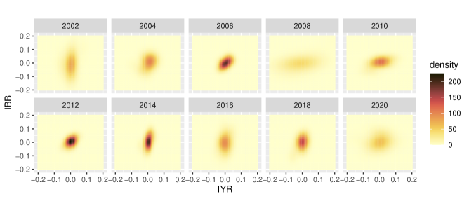
Figure S1: Kernel smoothed densities across different years for Biotechnology (IBB) and Real Estate (IYR) ETFs.

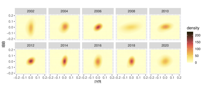
Figure S2: Fitted density surfaces for different years obtained by the LSWW version of sliced Wasserstein regression with sliced Wasserstein fraction of variance explained at level 0.95 for Biotechnology (IBB) and Real Estate (IYR) ETFs.

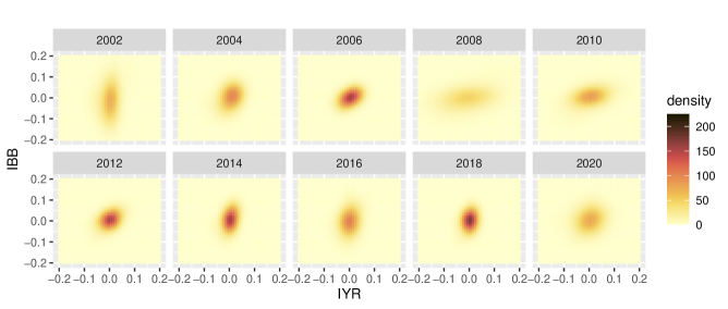
Figure S3: Fitted density surfaces for different years obtained by the LSAW version of sliced Wasserstein regression with sliced Wasserstein fraction of variance explained at level 0.74 for Biotechnology (IBB) and Real Estate (IYR) ETFs.

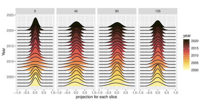
Figure S4: Fréchet regressions for LSWW between year (predictor, on the $y$-axis) and fitted slicing distributions (response, on the $x$-axis) for various projections. The number at the top of each panel indicates the angle of the respective projection with the $x$-axis (IYR) in Figure S1.

S.6 SLICING TRANSFORMS

Various slicing transforms besides the Radon transform may be of interest. One of these is the circular Radon transform $\mathcal{CR}$ (Kuchment, 2006). This transform is the integral of a function $f$ over a sphere centered at $\theta\in\Theta$, where

$$\mathcal{CR}(f)(\theta,u)=\int_{|z-\theta|=u}f(z)d\sigma(z),\quad\theta\in\Theta.$$

The injectivity property of the circular Radon transform has been studied previously, especially for the case when $\Theta$ is a unit sphere (Agranovsky and Quinto, 1996; Ehrenpreis, 2003). However, the analytic inverse formulas for even dimensions are still unknown (Finch and Patch, 2004).

Another transform of interest is the generalized Radon transform, which extends the classic Radon transform (Beylkin, 1984; Ehrenpreis, 2003). The generalized Radon transform $\mathcal{GR}$ is defined as an integral over $I_{u,\theta}=\{z\in D|\chi(z,\theta)=u\}$,

$$\mathcal{GR}\left(f\right)(\theta,u)=\int_{\chi(z,\theta)=u}f(z)d\sigma(z),$$

where $d\sigma(z)$ integrates the surface area on $I_{u,\theta}$ and $\chi$ is a so-called defining function if it satisfies some regularity conditions (Beylkin, 1984). The sliced Wasserstein distance has been extended to the generalized Radon transform (Kolouri et al., 2019).

S.7 AUXILIARY LEMMAS AND PROPOSITIONS

Lemma S1.

Assume (D1) and (F2). For any vector $\mathbf{k}=(k_{1},...,k_{p})$ of $p$ non-negative integers with $\sum_{l=1}^{p}k_{l}=k$ let $\mathcal{D}^{\mathbf{k}}=\frac{\partial^{k}}{\partial z_{k_{1}}\cdots\partial z_{k_{p}}}$. It holds that $\mathcal{R}(f)(\theta,\cdot),f\in\mathcal{F},$ is $k-$times differentiable, and

$$\mathcal{R}\left[\mathcal{D}^{\mathbf{k}}f\right](\theta,u)=(-1)^{k}\left(\prod_{l=1}^{p}\theta_{l}^{k_{l}}\right)\frac{\partial^{k}\left(\mathcal{R}(f)\right)}{\partial u^{k}}(\theta,u),$$ (S.10)

for each $\theta=(\theta_{1},...,\theta_{p})\in\Theta$. Furthermore,

$$\left|\frac{\partial^{k}(\mathcal{R}(f))}{\partial u^{k}}(\theta,u)\right|\leq B_{1}p^{k/2}<\infty,$$

for each $\theta\in\Theta$ where the constant $B_{1}$ does not depend on $f$ or $\theta$.

Proof.

Assumptions (D1) and (F2) imply $f$ has bounded support and continuous partial derivatives of order $k$, and formula (S.10) follows from Proposition 6.1.3 in Epstein (2007). For each $\theta=(\theta_{1},...,\theta_{p})\in\Theta$, $\sum_{j=1}^{p}\theta_{j}^{2}=1$,

$$\max_{j=1,..,p}|\theta_{j}|\geq p^{-1/2}.$$

Let $j(\theta)=\operatorname*{argmax}_{j=1,\cdots,p}|\theta_{j}|$. Taking $\mathbf{k}(\theta)=(0,...,0,k,0,...,0)$ with all components equal to $0$ except the $j(\theta)$-th as $k$, so that

$$\left|\left(\prod_{l=1}^{p}\theta_{l}^{k_{l}}\right)\right|=\left(\prod_{l=1}^{p}|\theta_{l}|^{k_{l}}\right)\geq p^{-k/2}.$$

Since $\norm{\mathcal{D}^{\mathbf{k}(\theta)}f}_{\infty}\leq B_{1}$ for a constant $B_{1}$ from (F2), it follows from the definition of the Radon transform that $\norm{\mathcal{R}\left[\mathcal{D}^{\mathbf{k}(\theta)}f\right](\theta,u)}_{\infty}\leq B_{1}$. Hence,

$$\absolutevalue{\frac{\partial^{k}\left(\mathcal{R}(f)\right)}{\partial u^{k}}(\theta,u)}\leq B_{1}p^{k/2}.$$

∎

Lemma S2.

Suppose $h_{1},h_{2}$ are three times continuously differentiable on [0,1] with
$\max\{\|h_{1}^{(3)}(s)\|_{\infty},\|h_{2}^{(3)}(s)\|_{\infty}\}\leq B_{0}$ where $B_{0}$ is a constant, then

$$|h_{1}^{\prime}(s)-h_{2}^{\prime}(s)|\leq C(B_{0})d_{2}^{4/7}(h_{1},h_{2}),\quad\forall z\in[0,1].$$

Proof.

From Lemma 1 in Chen et al. (2020), arbitrarily fix $s\in(0,1)$, and assume for the bandwidth $a$ that $a\leq\min\{s,1-s\}$. As $a\rightarrow 0$,

$$\int_{0}^{1}a^{-1}h_{1}(u)\mathcal{K}\left(\frac{s-u}{a}\right)du=h_{1}(s)+\frac{1}{2}a^{2}\sigma^{2}(\mathcal{K})h_{1}^{(2)}(s)+R_{11}(a),$$

$$\int_{0}^{1}a^{-2}h_{1}(u)\mathcal{K}^{\prime}\left(\frac{s-u}{a}\right)du=h_{1}^{\prime}(s)+\frac{1}{2}a^{2}\sigma^{2}(\mathcal{K})h_{1}^{(3)}(s)+R_{12}(a).$$

Consider a kernel function $\mathcal{K}(\cdot)$ that is a symmetric probability density function with compact support on [-1,1] and a bounded derivative $\mathcal{K}^{\prime}$. Furthermore, assume $\mathcal{K}$ satisfies that $\sigma^{2}(\mathcal{K})=\int u^{2}\mathcal{K}(u)du<\infty$ and $\sigma^{3}(\mathcal{K})=\int|u|^{3}\mathcal{K}(u)du<\infty$. Expanding $h_{1}(u)$,

$$h_{1}(u)=h_{1}(s)+h_{1}^{\prime}(s)(u-s)+h_{1}^{(2)}(s)(u-s)^{2}/2+\int_{s}^{u}\frac{h_{1}^{(3)}(t)(u-t)^{2}}{3!}dt.$$

The remainder terms $R_{11}(a),R_{12}(a)$ can be bounded as follows

$$\left|R_{11}(a)\right|=\left|\int_{0}^{1}a^{-1}\mathcal{K}\left(\frac{s-u}{a}\right)\int_{s}^{u}\frac{h_{1}^{(3)}(t)(u-t)^{2}}{3!}dtdu\right|\lesssim B_{0}a^{3},$$

$$R_{12}(a) =\int_{0}^{1}a^{-2}\mathcal{K}^{\prime}\left(\frac{s-u}{a}\right)\int_{s}^{u}\frac{h_{1}^{(3)}(t)(u-t)^{2}}{3!}dtdu$$

$$\quad-\int_{0}^{1}a^{-1}\mathcal{K}\left(\frac{s-u}{a}\right)\frac{h_{1}^{(3)}(s)(u-s)^{2}}{3!}du\lesssim B_{0}a^{2}.$$

Similarly for $h_{2}(u)$, we have

$$\int_{0}^{1}a^{-2}h_{2}(u)\mathcal{K}^{\prime}\left(\frac{s-u}{a}\right)du=h_{2}^{\prime}(s)+\frac{1}{2}a^{2}\sigma^{2}(\mathcal{K})h_{2}^{(3)}(s)+R_{22}(a).$$

Then

$$|h_{1}^{\prime}(s)-h_{2}^{\prime}(s)| \leq a^{-2}\int_{0}^{1}|h_{1}(u)-h_{2}(u)|\mathcal{K}^{\prime}\left(\frac{s-u}{a}\right)du+\frac{1}{2}a^{2}\sigma^{2}(\mathcal{K})|h_{1}^{(3)}(u)-h_{2}^{(3)}(u)|$$

$$\quad+\left|R_{12}(a)-R_{22}(a)\right|$$

$$\leq a^{-3/2}d_{2}(h_{1},h_{2})\left(\int\left(\mathcal{K}^{\prime}(u)\right)^{2}du\right)^{1/2}+B_{0}a^{2}\sigma^{2}(\mathcal{K})+\left|R_{12}(a)+R_{22}(a)\right|$$

$$\lesssim C_{1}(B_{0})\left(a^{-3/2}d_{2}(h_{1},h_{2})\right)+C_{2}(B_{0})a^{2},$$

for constants $C_{1}(B_{0}),C_{2}(B_{0})$ which only depend on $B_{0}$. By choosing $a\sim d_{2}^{2/7}(h_{1},h_{2})$,

$$|h_{1}^{\prime}(s)-h_{2}^{\prime}(s)|\leq C(B_{0})d_{2}^{4/7}(h_{1},h_{2}).$$

∎

Lemma S3.

If $D$ is compact, the univariate Wasserstein distance is bounded by the $L^{2}$ distance of the corresponding densities

$$d_{W}(\nu_{1},\nu_{2})\lesssim d_{2}\left(\varphi(\nu_{1}),\varphi(\nu_{2})\right),\quad\nu_{1},\nu_{2}\in\mathscr{G}.$$ (S.11)

Proof.

From Theorem 4 in Gibbs and Su (2002),

$$d_{W}(\nu_{1},\nu_{2})\leq\text{diam}(D)d_{TV}(\nu_{1},\nu_{2}),\quad\nu_{1},\nu_{2}\in\mathscr{G},$$

where $\text{diam}(D)=\sup\{d(z_{1},z_{2}):z_{1},z_{2}\in D\}$ and $d_{TV}(\nu_{1},\nu_{2})$ represents the total variation distance $d_{TV}=\sup_{S\subset D}|\nu_{1}(S)-\nu_{2}(S)|$. Note that when $\nu_{1}$ and $\nu_{2}$ have densities $\varphi(\nu_{1})$ and $\varphi(\nu_{2})$, it follows that

$$d_{TV}(\nu_{1},\nu_{2})=\frac{1}{2}\int_{D}|\varphi(\nu_{1})(u)-\varphi(\nu_{2})(u)|du\leq\frac{1}{2}\sqrt{\text{diam}(D)}d_{2}(\varphi(\nu_{1}),\varphi(\nu_{2})).$$

If $D$ is a compact set, $\text{diam}(D)$ is bounded. We conclude that

$$d_{W}(\nu_{1},\nu_{2})\lesssim d_{2}(\varphi(\nu_{1}),\varphi(\nu_{2})).$$ (S.12)

∎

Proposition S4.

Assume (T0) and (T2), for $m_{G}^{SAW}$ as per (14) and $M_{G}^{SWW}$ as per (16),

$$m_{G}^{SAW}(x)=\widetilde{\psi}^{-1}\left[\operatorname*{argmin}_{\gamma\in\Gamma_{\Theta}\cap\widetilde{\psi}(\mathscr{F})}M_{G}^{SWW}(\gamma,x)\right].$$

Similarly, for $m_{L,h}^{SAW}$ as per (S.4) and $M_{L,h}^{SWW}$ as per (S.5),

$$m_{L,h}^{SAW}(x)=\widetilde{\psi}^{-1}\left[\operatorname*{argmin}_{\gamma\in\Gamma_{\Theta}\cap\widetilde{\psi}(\mathscr{F})}M_{L,h}^{SWW}(\gamma,x)\right].$$

Proof.

The change of variable ${\gamma}=\widetilde{\psi}(\omega)\in\widetilde{\psi}(\mathscr{F})$, $\omega\in\mathscr{F}$ is a bijection because of the injectivity of the transform $\widetilde{\psi}$. Hence,

$$m_{G}^{SAW}(x) =\operatorname*{argmin}_{\omega\in\mathscr{F}}E\left[s_{G}(X,x)d_{SW}^{2}(\mu,\omega)\right]$$

$$=\operatorname*{argmin}_{\omega\in\mathscr{F}}E\left[s_{G}(X,x)d_{DW}^{2}(\widetilde{\psi}(\mu),\widetilde{\psi}(\omega))\right]$$

$$=\widetilde{\psi}^{-1}\left(\operatorname*{argmin}_{{\gamma}\in\Gamma_{\Theta}\bigcap\widetilde{\psi}(\mathscr{F})}E\left[s_{G}(X,x)d_{DW}^{2}(\widetilde{\psi}(\mu),\gamma)\right]\right)$$

$$=\widetilde{\psi}^{-1}\left[\operatorname*{argmin}_{{\gamma}\in\Gamma_{\Theta}\bigcap\widetilde{\psi}(\mathscr{F})}M_{G}^{SWW}(\omega,x)\right].$$

Similarly,

$$m_{L,h}^{SAW}(x)=\widetilde{\psi}^{-1}\left[\operatorname*{argmin}_{\gamma\in\Gamma_{\Theta}\cap\widetilde{\psi}(\mathscr{F})}M_{L,h}^{SWW}(\gamma,x)\right].$$

∎

S.8 PROOFS

S.8.1 Proof of Proposition 1

Proof.

First, we show that if assumptions (D1), (F1), and (F2) are satisfied, $\mathcal{R}(\mathcal{F})$ satisfies assumptions (D2), (G1) and (G2). It is clear that $\mathcal{R}(f)\geq 0$ and $\int_{u}\mathcal{R}(f)(\theta,u)du=1$, where we denote $\mathcal{R}(f)(\theta,u)$ as $\mathcal{R}(f)(\theta)(u)$ for simplicity. The validity of (D2) follows from (D1) and the definition of the Radon transform. Furthermore, (G1) can be deduced from (D1) and (F1), while (G2) holds based on (D1) and the implications of Lemma S1. Next, we prove that (T0) and (T1) are satisfied. The injectivity of the Radon transform is evident from the definition. Hence, (T0) is satisfied. Since $D$ is compact, there exists a constant $C$ such that $\norm{D}_{\infty}\leq C$. Computing the $L^{2}$-distance between $\mathcal{R}(f_{1})$ and $\mathcal{R}(f_{2})$ for fixed $\theta\in\Theta$,

$${\int_{\mathbb{R}}\absolutevalue{\mathcal{R}(f_{1})(\theta,u)-\mathcal{R}(f_{2})(\theta,u)}^{2}du}$$

$$=\int_{-C}^{C}\left(\int_{-C}^{C}\cdots\int_{-C}^{C}\left(\left(f_{1}-f_{2}\right)\left(u\theta+\sum_{j=1}^{p-1}s_{j}e_{j}\right)\right)ds_{1}\cdots ds_{p}\right)^{2}du$$

$$\leq(2C)^{p-1}\int_{-C}^{C}\cdots\int_{-C}^{C}\left(\left(f_{1}-f_{2}\right)\left(u\theta+\sum_{j=1}^{p-1}s_{j}e_{j}\right)\right)^{2}ds_{1}\cdots ds_{p}du$$

$$\leq(2C)^{p-1}d_{2}^{2}(f_{1},f_{2}).$$

The first inequality follows from the Cauchy-Schwarz inequality. Thus, (T1) holds as well. ∎

S.8.2 Proof of Theorem 1

Proof.

Set ${\widebar{\mathcal{R}(f)}(\theta,r)}=\mathcal{J}_{1}(\mathcal{R}(f)(\theta))(r)$, $r\in\mathbb{R}$ and $\check{\Delta}_{\tau,1}=f-\check{\mathcal{R}}_{\tau}(\mathcal{R}(f))$. Then we have

$$\check{\Delta}_{\tau,1} =\frac{1}{2(2\pi)^{p}}\int_{\Theta}\int_{|r|>\tau}\widebar{\mathcal{R}(f)}(\theta,r)e^{ir\langle\theta,z\rangle}|r|^{p-1}drd\theta.$$

Since $\mathcal{R}(f)(\theta)(\cdot)$ has uniform bounded $k$-derivative for each $\theta\in\Theta$ from (G2), it follows from Proposition 3.2.2 in Epstein (2007) that

$$|\widebar{\mathcal{R}(f)}(\theta,r)|\leq M_{3}|r|^{-k},$$

where $M_{3}$ is a constant such that $\|\mathcal{R}(f)(\theta)(\cdot)\|_{\infty}\leq M_{3}$. Therefore, we get

$$\norm{\check{\Delta}_{\tau,1}}_{\infty} \leq\frac{1}{2(2\pi)^{p}}\int_{\Theta}\int_{|r|>\tau}\absolutevalue{\widebar{\mathcal{R}(f)}(\theta,r)}|r|^{p-1}drd\theta$$

$$\leq\frac{M_{3}}{2(2\pi)^{p}}\int_{\Theta}d\theta\int_{|r|>\tau}|r|^{p-k-1}dr$$

$$=O\left(\tau^{-(k-p)}\right),$$

where we note that $k\geq p+1$ from (F2). Since $\int_{D}f(z)dz=1>0$ and $\|f\|_{\infty}\leq M_{0}$ from (F1), we obtain $\|\Delta_{\tau,1}\|_{\infty}=O\left(\tau^{-(k-p)}\right)$.

Next, set ${\lambda_{f}=\mathcal{R}(f)}$, $\lambda_{f}^{*}=\widetilde{\mathcal{R}(f)}\in\Lambda_{\Theta}$ and $\check{\Delta}_{\tau,2}=\check{\mathcal{R}}^{-1}_{\tau}(\lambda_{f})-\check{\mathcal{R}}^{-1}_{\tau}(\lambda_{f}^{*})$, yielding

$$\norm{\check{\Delta}_{\tau,2}}_{\infty} =\frac{1}{2(2\pi)^{p}}\int_{\Theta}\int_{|r|\leq\tau}(\widebar{\lambda_{f}}(\theta,r)-\widebar{\lambda_{f}^{*}}(\theta,r))|r|^{p-1}e^{ir\langle\theta,z\rangle}drd\theta$$

$$\leq\frac{\tau^{p-1}}{2(2\pi)^{p}}\int_{\Theta}\int_{|r|\leq\tau}\absolutevalue{\widebar{\lambda_{f}}(\theta,r)-\widebar{\lambda_{f}^{*}}(\theta,r)}drd\theta$$

$$\leq\frac{\tau^{p-1}}{2(2\pi)^{p}}\int_{\Theta}\int_{|r|\leq\tau}\int_{\mathbb{R}}|\lambda_{f}(\theta,u)-\lambda_{f}^{*}(\theta,u)|dudrd\theta$$

$$\lesssim\frac{\tau^{p}}{2(2\pi)^{p}}d_{2}(\lambda_{f},\lambda_{f}^{*}).$$

The last inequality follows from the bounded support of $\Lambda_{\Theta}$ and $\mathcal{F}$. Note that $\|\check{\mathcal{R}}_{\tau}(\mathcal{R}(f))-f\|_{\infty}=O\left(\tau^{-(k-p)}\right)$ as $\tau\rightarrow\infty$. The boundedness of $\Delta_{\tau,2}$ follows from the fact $\int_{D}f(z)dz=1$ and the condition that $d_{2}(\lambda_{f}^{*},\lambda_{f})\rightarrow 0$, whence

$$\norm{\Delta_{\tau,2}}_{\infty}=O\left(\tau^{p}d_{2}(\lambda_{f},\lambda_{f}^{*})\right)=O\left(\tau^{p}d_{2}\left({\mathcal{R}(f),\widetilde{\mathcal{R}(f)}}\right)\right).$$

∎

S.8.3 Proof of Proposition 3

This proof follows a similar approach as Proposition 1 of Kolouri et al. (2019), but we present it for a more generalized version of the slicing transform as follows. If $\mu_{1}=\mu_{2},\,\mu_{1},\mu_{2}\in\mathscr{F}$, the slice-averaged Wasserstein distance satisfies $d_{SW}(\mu_{1},\mu_{2})=0$. The non-negativity and symmetry properties of the slice-averaged Wasserstein distance are direct consequences of the Wasserstein distance being a metric. We next consider the triangle inequality. For any $\mu_{1},\mu_{2},\mu_{3}\in\mathscr{F}$,

$$d_{SW}(\mu_{1},\mu_{3}) =\left(\int_{\Theta}d_{W}^{2}(G^{-1}\left(\widetilde{\psi}(\mu_{1})(\theta)\right),G^{-1}\left(\widetilde{\psi}(\mu_{3})(\theta)\right))\right)^{1/2}$$

$$\leq\left(\int_{\Theta}d_{W}^{2}(G^{-1}\left(\widetilde{\psi}(\mu_{1})(\theta)\right),G^{-1}\left(\widetilde{\psi}(\mu_{2})(\theta)\right))\right)^{1/2}$$

$$\quad+\left(\int_{\Theta}d_{W}^{2}(G^{-1}\left(\widetilde{\psi}(\mu_{2})(\theta)\right),G^{-1}\left(\widetilde{\psi}(\mu_{3})(\theta)\right))\right)^{1/2}$$

$$=d_{SW}(\mu_{1},\mu_{2})+d_{SW}(\mu_{2},\mu_{3})$$

The last inequality is obtained using the Minkowski inequality. We have thus established that the slice-averaged Wasserstein distance satisfies non-negativity, symmetry and the triangle inequality, hence it is a pseudo-metric. If $d_{SW}(\mu_{1},\mu_{2})=0$,

$$d_{W}\left(G^{-1}\left(\widetilde{\psi}(\mu_{1})(\theta)\right),G^{-1}\left(\widetilde{\psi}(\mu_{2})(\theta)\right)\right)=0,\quad\text{for almost all }\theta\in\Theta.$$

Equivalently, considering that the Wasserstein distance is a metric, we have $\widetilde{\psi}(\mu_{1})=\widetilde{\psi}(\mu_{2})$. Therefore, the slice-averaged Wasserstein distance is a distance if and only if $\widetilde{\psi}(\mu_{1})=\widetilde{\psi}(\mu_{2})$ implies $\mu_{1}=\mu_{2}$, which is equivalent to the injectivity of $\widetilde{\psi}$. Note that $\widetilde{\psi}$ is induced from $\psi$, and since $\varphi$ and $\varrho$ are bijective, the injectivity of $\widetilde{\psi}$ is equivalent to (T0).

S.8.4 Proof of Proposition 4 and Proposition S2

Proof.

For any $\gamma_{1},\gamma_{2}\in\Gamma_{\Theta}$,

$$d_{DW}^{2}(\gamma_{1},\gamma_{2}) =\int_{\Theta}d_{W}^{2}(G^{-1}\left(\gamma_{1}(\theta)\right),G^{-1}\left(\gamma_{2}(\theta)\right))d\theta$$

$$\lesssim\int_{\Theta}d_{2}^{2}(\varrho(\gamma_{1})(\theta),\varrho(\gamma_{2})(\theta))d\theta,$$

$$\lesssim\int_{\Theta}d_{\infty}^{2}(\varrho(\gamma_{1})(\theta),\varrho(\gamma_{2})(\theta))d\theta.$$

The first inequality comes from the distance relationship discussed in Lemma S3. Following the boundedness condition in (D1) and (G1), $d_{DW}(\gamma_{1},\gamma_{2})$ is bounded from above. Therefore,

$$\quad E\left[s_{G}(X,x)d_{DW}^{2}(\widetilde{\psi}(\mu),\gamma)\right]$$

$$=\int_{X,\mu}s_{G}(X,x)\int_{\Theta}d_{W}^{2}\left(G^{-1}\left(\widetilde{\psi}(\mu)(\theta)\right),G^{-1}\left(\gamma(\theta)\right)\right)d\theta d_{F}(X,\mu)$$

$$=\int_{\Theta}\int_{X,\mu}s_{G}(X,x)d_{W}^{2}\left(G^{-1}\left(\widetilde{\psi}(\mu)(\theta)\right),G^{-1}\left(\gamma(\theta)\right)\right)d_{F}(X,\mu)d\theta$$

$$=\int_{\Theta}E\left[s_{G}(X,x)d_{W}^{2}\left(G^{-1}\left(\widetilde{\psi}(\mu)(\theta)\right),G^{-1}\left(\gamma(\theta)\right)\right)\right]d\theta.$$

Since $s_{G}(X,x)>0$, the second equation follows from the Fubini theorem. The last equation indicates that finding the minimum in $E\left[s_{G}(X,x)d_{DW}^{2}(\widetilde{\psi}(\mu),\gamma)\right]$ is equivalent to finding the minimum in $E\left[s_{G}(X,x)d_{W}^{2}\left(G^{-1}\left(\widetilde{\psi}(\mu)(\theta)\right),G^{-1}\left(\gamma(\theta)\right)\right)\right]$ for almost all $\theta\in\Theta$. The result for the local slice-wise Wasserstein regression can be derived analogously. ∎

S.8.5 Proof of Proposition S1

Proof.

Set $z=(z_{1},...,z_{p})^{T}\in\mathbb{R}^{p}$ and $t=(t_{1},...,t_{p})^{T}\in\mathbb{R}^{p}$. We can express the expected value as follows

$$E\left[\hat{f}(z)\middle|f\right] =\frac{1}{\prod_{s=1}^{p}b_{s}}\int\prod_{s=1}^{p}\kappa\left(\frac{z_{s}-t_{s}}{b_{s}}\right)f(t_{1},...,t_{p})dt_{1},...,dt_{p}.$$ (S.13)

Expanding the multivariate density function $f(t)$ yields

$$f(t)=f(z)+\sum_{s=1}^{p}\frac{\partial f(z)}{\partial z_{s}}(t_{s}-z_{s})+\sum_{s_{1}=1}^{p}\sum_{s_{2}=1}^{p}\frac{\partial f^{2}(z^{*})}{\partial z_{s_{1}}z_{s_{2}}}(t_{s_{1}}-z_{s_{1}})(t_{s_{2}}-z_{s_{2}})/2,$$

where $z^{*}=z+\alpha(t-z)$ for a $\alpha\in(0,1)$. With (S.13),

$$E\left[\hat{f}(z)\middle|f\right]=f(z)+\frac{1}{2}\sum_{s=1}^{p}\int b_{s}^{-1}\frac{\partial^{2}f(z^{*})}{\partial z_{s}^{2}}\kappa\left(\frac{z_{s}-t_{s}}{b_{s}}\right)(z_{s}-t_{s})^{2}dt_{s}.$$

Here we use the symmetry property (K1) of the kernel function which implies $\int_{\mathbb{R}}u\kappa(u)du=0$. From (F2), there exists a constant $M_{3}$ that does not depend on the function $f$ such that the partial derivative $|\partial^{2}f(z^{*})/\partial z_{s}^{2}|$ is uniformly bounded by $M_{3}$ for $s=1,...,p$. Then

$$\sup_{f\in\mathcal{F}}\left|E\left[\hat{f}(z)\middle|f\right]-f(z)\right|=O(\sum_{s=1}^{p}b_{s}^{2}),$$

where we use (K2). Next, we establish the boundedness of the variance of $\hat{f}(z)$,

$$\operatorname*{Var}\left(\hat{f}(z)\middle|f\right) =\frac{1}{N}\operatorname*{Var}\left(\prod_{s=1}^{p}\kappa\left(\frac{z_{s}-Z_{js}}{b_{s}}\right)b_{s}^{-1}\middle|f\right)$$

$$\leq\frac{1}{N}\int\dots\int\prod_{s=1}^{p}\kappa\left(\frac{z_{s}-t_{s}}{b_{s}}\right)^{2}b_{s}^{-2}f(t_{1},...,t_{p})dt_{1}\cdots dt_{p}$$

$$\leq\frac{M_{0}}{N}\prod_{s=1}^{p}\int\kappa\left(\frac{z_{s}-t_{s}}{b_{s}}\right)^{2}b_{s}^{-2}dt_{s},$$

where $M_{0}$ from assumption (F1) is a constant that does not depend on the density function $f$. From (K2),

$$\sup_{f\in\mathcal{F}}\operatorname*{Var}\left(\hat{f}(z)\middle|f\right)=O\left(\frac{1}{N\prod_{s=1}^{p}b_{s}}\right).$$

Combining the above results, we obtain

$$\sup_{f\in\mathcal{F}}E\left(d_{2}(f,\hat{f})\middle|f\right)=O\left(\frac{1}{N\prod_{s=1}^{p}b_{s}}+\left(\sum_{s=1}^{p}b_{s}^{2}\right)^{2}\right).$$

Choosing $b_{s}\sim N^{-\frac{1}{p+4}}$ leads to

$$\sup_{f\in\mathcal{F}}E\left(d_{2}(f,\hat{f})\middle|f\right)=O\left(N^{-4/(4+p)}\right).$$

∎

S.8.6 Proof of Theorem 2

Proof.

The proof proceeds in two steps.

Step 1. We first prove $d_{SW}\left(m_{G}^{SAW}(x),\check{m}_{G}^{SAW}(x)\right)=O_{p}\left(n^{-1/2}\right)$ and establish the following three properties for the SAW estimator $\check{m}_{G}^{SAW}(x)$.

(R1): The objects $m_{G}^{SAW}(x)$ and $\check{m}_{G}^{SAW}(x)$ exist and are unique, the latter almost surely, and, for any $\epsilon>0$,

$$\inf_{d_{SW}\left(m_{G}^{SAW}(x),\omega\right)>\epsilon}M_{G}^{SAW}(\omega,x)>M_{G}^{SAW}\left(m_{G}^{SAW}(x),x\right).$$

(R2): Let $B_{\delta}\left[m_{G}^{SAW}(x)\right]$ be the $\delta$-ball in $\mathscr{F}$ centered at $m_{G}^{SAW}(x)$ and $N(\epsilon,\mathscr{F},d_{SW})$ its covering number using balls of size $\epsilon$. Then

$$\int_{0}^{1}\left(1+\log N\left\{\delta\epsilon,B_{\delta}\left[m_{G}^{SAW}(x)\right],d_{SW}\right\}\right)^{1/2}d\epsilon=O(1)\quad\text{ as }\delta\rightarrow 0\text{. }$$

(R3) There exists $\eta_{0}>0,\beta_{0}>0,$ possibly depending on $x$, such that

$$\inf_{d_{SW}\left(m_{G}^{SAW}(x),\omega\right)<\eta_{0}}\left\{M_{G}^{SAW}(\omega,x)-M_{G}^{SAW}\left(m_{G}^{SAW}(x),x\right)-\beta_{0}d_{SW}\left(m_{G}^{SAW}(x),\omega\right)^{2}\right\}\geq 0.$$

Proof of (R2): We note that $d_{W}^{2}(\nu_{1},\nu_{2})=O(d_{2}(\varphi(\nu_{1}),\varphi(\nu_{2})))$ from Lemma S3, whence

$$d_{SW}(\mu_{1},\mu_{2}) =\left(\int_{\Theta}d_{W}^{2}(G^{-1}\left(\widetilde{\psi}(\mu_{1})(\theta)\right),G^{-1}\left(\widetilde{\psi}(\mu_{2})(\theta)\right))d\theta\right)^{1/2}$$

$$\lesssim\left(\int_{\Theta}d_{2}^{2}(\psi\circ\varphi(\mu_{1})(\theta),\psi\circ\varphi(\mu_{2})(\theta))d\theta\right)^{1/2}$$

$$\lesssim d_{2}(\varphi(\mu_{1}),\varphi(\mu_{2})),$$ (S.14)

where the last inequality follows from (T1) and the compactness of $\Theta$. Using Theorem 2.7.1 of Vaart and Wellner (1996), there exists a constant $A_{1}$ depending only on $k$ and $p$ such that

$$\log N(\epsilon,\mathcal{F},\|\|_{\infty})\leq A_{1}{\epsilon}^{-p/k},$$

for every $\epsilon>0$ and $k\geq p+1$ from (F2). Note that $d_{SW}(\mu_{1},\mu_{2})=O(d_{2}(\varphi(\mu_{1}),\varphi(\mu_{2})))=O(d_{\infty}(\varphi(\mu_{1}),\varphi(\mu_{2}))$ and from the boundedness of the support set $D$, we have $B_{A_{2}\epsilon}(\mu,\|\|_{\infty})\subset B_{\epsilon}(\mu,d_{SW})$ for some constant $A_{2}$. Thus, we have $N(\epsilon,\mathscr{F},d_{SW})\leq A_{3}N(\epsilon,\mathcal{F},\|\|_{\infty})$. It follows that

$$\int_{0}^{1}\sqrt{1+\log N\{\delta\epsilon,B_{\delta}[m_{G}^{SAW}(x)],d_{SW}\}}d\epsilon <\int_{0}^{1}\sqrt{1+\log N\{\delta\epsilon,\mathscr{F},d_{SW}\}}d\epsilon$$

$$\leq\int_{0}^{1}\sqrt{1+A_{3}A_{1}\epsilon^{-p/k}}<\infty.$$ (S.15)

Proof of (R1) and (R3): We define the Hilbert space $\mathcal{H}$ as the set of all functions

$$\mathcal{H}:=\{\varsigma\in\mathcal{H}:\Theta\times[0,1]\rightarrow\mathbb{R},\int_{\Theta}\int_{[0,1]}\varsigma^{2}(\theta,s)dsd\theta<\infty\}$$

with the inner product

$$\langle\varsigma_{1},\varsigma_{2}\rangle=\int_{\Theta}\int_{[0,1]}\varsigma_{1}(\theta,s)\varsigma_{2}(\theta,s)dsd\theta.$$

Here the integral is well defined due to the Cauchy-Schwarz inequality. It is easy to verify that the space $\mathcal{H}$ is a vector space over the field $\mathbb{R}$. The inner product satisfies the conditions of conjugate symmetry, linearity, and positive definiteness. The compactness of the Hilbert space follows from the fact that $\mathcal{H}$ consists of measurable functions that are square integrable. We define the $L^{2}$ distance between two functions $\varsigma_{1},\varsigma_{2}\in\mathcal{H}$ as $d_{2}(\varsigma_{1},\varsigma_{2})=\langle\varsigma_{1}-\varsigma_{2},\varsigma_{1}-\varsigma_{2}\rangle$. Note that the quantile slicing space $\Gamma_{\Theta}$ is a subspace of $\mathcal{H}$ and the distribution slicing Wasserstein metric coincides with the $L^{2}$ distance, i.e., $d_{DW}(\gamma_{1},\gamma_{2})=d_{2}(\gamma_{1},\gamma_{2})$ for $\gamma_{1},\gamma_{2}\in\Gamma_{\Theta}$. Let $B_{G}(x)=E[s_{G}(X,x)\widetilde{\psi}(\mu)]$, then for any fixed $\omega\in\mathscr{F}$,

$$M_{G}^{SAW}(\omega,x) =E[s_{G}(X,x)d_{SW}^{2}(\mu,\omega)]$$

$$=E[s_{G}(X,x)d_{2}^{2}(\widetilde{\psi}(\mu),\widetilde{\psi}(\omega))]$$

$$=E[s_{G}(X,x)\langle\widetilde{\psi}(\mu)-\widetilde{\psi}(\omega),\widetilde{\psi}(\mu)-\widetilde{\psi}(\omega)\rangle]$$

$$=E[s_{G}(X,x)\langle\widetilde{\psi}(\mu)-B_{G}(x),\widetilde{\psi}(\mu)-B_{G}(x)\rangle]$$

$$\qquad+E[s_{G}(X,x)\langle B_{G}(x)-\widetilde{\psi}(\omega),B_{G}(x)-\widetilde{\psi}(\omega)\rangle]$$

$$\qquad+2E[s_{G}(X,x)\langle\widetilde{\psi}(\mu)-B_{G}(x),B_{G}(x)-\widetilde{\psi}(\omega)\rangle]$$

$$=E[s_{G}(X,x)d_{2}^{2}(\widetilde{\psi}(\mu),B_{G}(x))]+E[s_{G}(X,x)d_{2}^{2}(B_{G}(x),\widetilde{\psi}(\omega))]$$

$$=E[s_{G}(X,x)d_{2}^{2}(\widetilde{\psi}(\mu),B_{G}(x))]+d_{2}^{2}(B_{G}(x),\widetilde{\psi}(\omega)),$$

where the last equation follows from the fact that $E[s_{G}(X,x)]=1$. Thus,

$$m_{G}^{SAW}(x)=\operatorname*{argmin}_{\omega\in\mathscr{F}}d_{2}^{2}(B_{G}(x),\widetilde{\psi}(\omega)).$$

Using $n^{-1}\sum_{i=1}^{n}s_{iG}(x)=1$, one can similarly show that

$$\check{m}_{G}^{SAW}(x)=\operatorname*{argmin}_{\omega\in\mathscr{F}}d_{2}^{2}(\check{B}_{G}(x),\widetilde{\psi}(\omega)),$$ (S.16)

where $\check{B}_{G}(x)=n^{-1}\sum_{i=1}^{n}s_{iG}(x)\widetilde{\psi}(\mu_{i})$. From the convexity and closedness of space $\widetilde{\psi}(\mathscr{F})$, the minimizers $m_{G}^{SAW}(x)$ and $\check{m}_{G}^{SAW}(x)$ exist and are unique for any $x\in\mathbb{R}^{q}$, so that (R1) is satisfied. The best approximation $m_{G}^{SAW}(x)\in\mathscr{F}$ can be characterized by (Deutsch, 2012, chap.4)

$$\langle B_{G}(x)-\widetilde{\psi}(m_{G}^{SAW}(x)),\widetilde{\psi}(\omega)-\widetilde{\psi}(m_{G}^{SAW}(x))\rangle\leq 0,\text{ for all }\omega\in\mathscr{F}.$$ (S.17)

Consequently, $d_{2}^{2}(B_{G}(x),\widetilde{\psi}(\omega))\geq d_{2}^{2}(B_{G}(x),\widetilde{\psi}(m_{G}^{SAW}(x)))+d_{2}^{2}(\widetilde{\psi}(m_{G}^{SAW}(x)),\widetilde{\psi}(\omega))$. Then,

$$M_{G}^{SAW}(\omega,x) \geq M_{G}^{SAW}(m_{G}^{SAW}(x),x)+d_{2}^{2}(\widetilde{\psi}(m_{G}^{SAW}(x)),\widetilde{\psi}(\omega))$$

$$=M_{G}^{SAW}(m_{G}^{SAW}(x),x)+d_{SW}^{2}(m_{G}^{SAW}(x),\omega),$$

for all $\omega\in\mathscr{F}$. Hence, we may choose $\beta_{0}=1$.

Under Properties (R1)-(R3), it follows from Petersen and Müller (2019) that

$$d_{SW}(m_{G}^{SAW}(x),\check{m}_{G}^{SAW}(x))=O_{p}(n^{-1/2}).$$ (S.18)

Step 2. Here we show that $d_{SW}(m_{G}^{SAW}(x),\hat{m}_{G}^{SAW}(x))=O_{p}(n^{-1/2})$. As before, $\varphi(\mu_{i})$ and $\varphi(\hat{\mu}_{i})$ denote the density functions of the $i$-th sample distribution $\mu_{i}$ and the estimator $\hat{\mu}_{i}$ (see (S.1)). From Proposition S1,

$$\max_{i=1,...,n}d_{2}(\varphi(\mu_{i}),\varphi(\hat{\mu}_{i}))=O_{p}\left(N^{-4/(4+p)}\right),$$

and the derivation of (S.14) implies

$$d_{2}(\widetilde{\psi}(\mu_{i}),\widetilde{\psi}(\hat{\mu}_{i}))=d_{SW}(\mu_{i},\hat{\mu}_{i})\lesssim d_{2}\left(\varphi(\mu_{i}),\varphi(\hat{\mu}_{i})\right).$$

Consequently,

$$\max_{i=1,...,n}d_{2}(\widetilde{\psi}(\mu_{i}),\widetilde{\psi}(\hat{\mu}_{i}))=O_{p}\left(N^{-4/(4+p)}\right).$$

Setting $\hat{B}_{G}(x)=n^{-1}\sum_{i=1}^{n}s_{iG}(x)\widetilde{\psi}(\hat{\mu}_{i})$ and noting that $n^{-1}\sum_{i=1}^{n}s_{iG}(x)=1$,

$$d_{2}(\check{B}_{G}(x),\hat{B}_{G}(x))=O_{p}\left(N^{-4/(4+p)}\right).$$

Similarly from the derivation of (S.16), we have

$$\hat{m}_{G}^{SAW}(x)=\operatorname*{argmin}_{\omega\in\mathscr{F}}d_{2}(\hat{B}_{G}(x),\widetilde{\psi}(\omega)).$$

By Theorem 5.3 of Deutsch (2012), considering the closeness and convexity of $\widetilde{\psi}(\mathcal{F})$, we obtain

$$d_{2}(\widetilde{\psi}(\check{m}_{G}^{SAW}(x)),\widetilde{\psi}(\hat{m}_{G}^{SAW}(x)))=O_{p}\left(N^{-4/(4+p)}\right),$$

whence

$$d_{SW}\left(\check{m}_{G}^{SAW}(x),\hat{m}_{G}^{SAW}(x)\right)=O_{p}\left(N^{-4/(4+p)}\right).$$ (S.19)

From (S.18) and assumption (P1), we conclude that

$$d_{SW}(m_{G}^{SAW}(x),\hat{m}_{G}^{SAW}(x))=O_{p}(n^{-1/2}).$$

Uniform convergence results require stronger versions of these properties provided by (R4)-(R6) as stated below. Let $\|\cdot\|_{E}$ be the Euclidean norm on $\mathbb{R}^{q}$ and $B>0$ a constant.

(R4) Almost surely, for all $\|x\|_{E}\leq B$, the objects $m_{G}^{SAW}(x)$ and $\check{m}_{G}^{SAW}(x)$ exist and are unique. Additionally, for any $\epsilon>0$,

$$\inf_{\|x\|_{E}\leq B}\inf_{d_{SW}\left(m_{G}^{SAW}(x),\omega\right)>\epsilon}\left\{M_{G}^{SAW}(\omega,x)-M_{G}^{SAW}\left[m_{G}^{SAW}(x),x\right]\right\}>0$$

and there exists $\zeta=\zeta(\epsilon)>0$ such that

$$\operatorname{pr}\left(\inf_{\|x\|_{E}\leq B}\inf_{d_{SW}\left[\check{m}_{G}^{SAW}(x),\omega\right]>\epsilon}\left\{\check{M}_{G}^{SAW}(\omega,x)-\check{M}_{G}^{SAW}\left[\check{m}_{G}^{SAW}(x),x\right]\right\}\geq\zeta\right)\rightarrow 1.$$

(R5) With $B_{\delta}[m_{G}^{SAW}(x)]$ and $N\left\{\epsilon,B_{\delta}\left[m_{G}^{SAW}(x)\right],d_{SW}\right\}$ as in condition (R2),

$$\int_{0}^{1}\sup_{\|x\|_{E}\leq B}\left(1+\log N\left\{\delta\epsilon,B_{\delta}\left[m_{G}^{SAW}(x)\right],d_{SW}\right\}\right)^{1/2}d\epsilon=O(1)\quad\text{ as }\delta\rightarrow 0.$$

(R6) There exist $\tau_{0}>0$, $C_{0}>0$, possibly depending on $B$, such that

$$\inf_{\begin{subarray}{c}\|x\|_{E}\leq B,\\ d_{SW}\left(m_{G}^{SAW}(x),\omega\right)<\tau_{0}\end{subarray}}\left\{M_{G}^{SAW}(\omega,x)-M_{G}\left[m_{G}^{SAW}(x),x\right]-C_{0}d_{SW}\left[m_{G}^{SAW}(x),\omega\right]^{2}\right\}\geq 0.$$

The derivation of (R1) and (R3) lead to (R4) and (R6) with $C_{0}=1$. From equation (S.8.6), we find that (R5) is satisfied. From Theorem 2 of Petersen and Müller (2019), we conclude that

$$\sup_{\|x\|_{E}\leq B}d_{SW}\left(m_{G}^{SAW}(x),\check{m}_{G}^{SAW}(x)\right)=O_{p}\left(n^{-1/(2+\epsilon)}\right).$$

Note that formula (S.19) is uniform for $\|x\|\leq B$, leading to

$$\sup_{\|x\|_{E}\leq B}d_{SW}\left(m_{G}^{SAW}(x),\hat{m}_{G}^{SAW}(x)\right)=O_{p}\left(n^{-1/(2+\epsilon)}\right).$$

∎

S.8.7 Proof of Theorem S1

Proof.

We first show that

$$d_{SW}\left(m^{SAW}(x),m_{L,h}^{SAW}(x)\right)=O\left(h^{2}\right),$$ (S.20)

$$d_{SW}\left(m_{L,h}^{SAW}(x),\check{m}_{L,h}^{SAW}(x)\right)=O_{p}\left(\left(nh\right)^{-1/2}\right).$$ (S.21)

We establish the following three properties for the SAW estimator $\check{m}_{L,h}^{SAW}(x)$.

(U1) The minimizers $m^{SAW}(x),m^{SAW}_{L,h}(x)$ and $\check{m}_{L,h}^{SAW}(x)$ exist and are unique, the last almost surely. Additionally, for any $\epsilon>0$,

$$\inf_{d_{SW}\left(m^{SAW}(x),\omega\right)>\epsilon}\{M^{SAW}(\omega,x)-M^{SAW}[m^{SAW}(x),x]\}>0,$$

$$\liminf_{h\rightarrow 0}\inf_{d_{SW}\left(m^{SAW}_{L,h}(x),\omega\right)>\epsilon}\left\{M^{SAW}_{L,h}(\omega,x)-M^{SAW}_{L,h}\left[m^{SAW}_{L,h}(x),x\right]\right\}>0.$$

(U2) Let $B_{\delta}[m^{SAW}(x)]$ be the ball of radius $\delta$ centered at $m^{SAW}(x)$ with covering number $N\left\{\delta\epsilon,B_{\delta}[m^{SAW}(x)],d_{SW}\right\}$. Then

$$\int_{0}^{1}\left(1+\log N\left\{\delta\epsilon,B_{\delta}[m^{SAW}(x)],d_{SW}\right\}\right)^{1/2}d\epsilon=O(1)\quad\text{ as }\delta\rightarrow 0.$$

(U3) There exists $\eta_{1},\eta_{2}>0$, $\beta_{1},\beta_{2}>0$ such that

$$\inf_{d_{SW}\left(m^{SAW}(x),\omega\right)<\eta_{1}}\left\{M^{SAW}(\omega,x)-M^{SAW}[m^{SAW}(x),x]-\beta_{1}d_{SW}\left(m^{SAW}(x),\omega\right)^{2}\right\}\geq 0,\\ \liminf_{h\rightarrow 0}\inf_{d_{SW}\left(m^{SAW}_{L,h}(x),\omega\right)<\eta_{2}}\left\{M^{SAW}_{L,h}(\omega,x)-M^{SAW}_{L,h}\left[m^{SAW}_{L,h}(x),x\right]\right.\\ \left.-\beta_{2}d_{SW}\left(m^{SAW}_{L,h}(x),\omega\right)^{2}\right\}\geq 0.$$

Proof of (U2). Similar to the derivation of (S.8.6), we have

$$\int_{0}^{1}\sqrt{1+\log N\{\delta\epsilon,B_{\delta}[m^{SAW}(x)],d_{SW}\}}d\epsilon <\int_{0}^{1}\sqrt{1+\log N\{\delta\epsilon,\mathscr{F},d_{SW}\}}d\epsilon$$

$$\leq\int_{0}^{1}\sqrt{1+A_{3}A_{1}\epsilon^{-p/k}}d\epsilon<\infty.$$

Proof of (U1) and (U3). For any distribution $\mu\in\mathscr{F}$, let $\widetilde{\psi}(\mu)\in\widetilde{\psi}(\mathscr{F})$ and $B(x)=E[\widetilde{\psi}(\mu)|X=x]$. Then

$$M^{SAW}(\omega,x) =E[d_{SW}^{2}(\mu,\omega)|X=x]$$

$$=E[d_{2}^{2}(\widetilde{\psi}(\mu),\widetilde{\psi}(\omega))|X=x]$$

$$=E[d_{2}^{2}(\widetilde{\psi}(\mu),B(x))|X=x]+E[d_{2}^{2}(B(x),\widetilde{\psi}(\omega))|X=x]$$

$$=M^{SAW}\left[B(x),x\right]+d_{2}^{2}\left(B(x),\widetilde{\psi}(\omega)\right)$$

for all $\omega\in\mathscr{F}$, whence

$$m^{SAW}(x)=\operatorname*{argmin}_{\omega\in\mathscr{F}}d_{2}^{2}\left(B(x),\widetilde{\psi}(\omega)\right).$$

Set $B_{L,h}(x)=E\left[s_{L}(X,x,h)\widetilde{\psi}(\mu)\right],\check{B}_{L,h}(x)=n^{-1}\sum_{i=1}^{n}s_{iL,h}(x)\widetilde{\psi}(\mu_{i})$. Considering $E[s_{L}(x,h)]=1$ and $n^{-1}\sum_{i=1}^{n}s_{iL,h}(x)=1$, one finds

$$m^{SAW}_{L,h}(x)=\operatorname*{argmin}_{\omega\in\mathscr{F}}d_{2}^{2}\left(B_{L,h}(x),\widetilde{\psi}(\omega)\right),$$

$$\check{m}^{SAW}_{L,h}(x)=\operatorname*{argmin}_{\omega\in\mathscr{F}}d_{2}^{2}\left(\check{B}_{L,h}(x),\widetilde{\psi}(\omega)\right).$$

From the convexity and closedness of space $\widetilde{\psi}(\mathscr{F})$, the minimizers $m^{SAW}(x)$, $m_{L,h}^{SAW}(x)$ and $\check{m}_{L,h}^{SAW}(x)$ exist uniquely for any $x\in\mathbb{R}$, so that (U1) is satisfied. Following the characterization of the best approximation as per (S.17), we have

$$M^{SAW}(\omega,x)\geq M^{SAW}\left(m^{SAW}(x),x\right)+d_{SW}^{2}\left(m^{SAW}(x),\omega\right).$$

Similarly,

$$M^{SAW}_{L,h}(\omega,x)\geq M^{SAW}_{L,h}\left(m^{SAW}_{L,h}(x),x\right)+d_{SW}^{2}\left(m^{SAW}_{L,h}(x),\omega\right).$$

Thus, (U3) is satisfied with $\beta_{1}=\beta_{2}=1$ and $\eta_{1},\eta_{2}$ chosen arbitrarily. Under conditions (L1)-(L2) and (U1)-(U3), it follows from Theorem 3 and Theorem 4 in Petersen and Müller (2019) that

$$d_{SW}\left(m^{SAW}(x),m_{L,h}^{SAW}(x)\right)=O\left(h^{2}\right),$$

$$d_{SW}\left(m_{L,h}^{SAW}(x),\check{m}_{L,h}^{SAW}(x)\right)=O_{p}\left(\left(nh\right)^{-1/2}\right).$$

Hence, we conclude that (S.20) and (S.21) are satisfied. Similarly to the derivation of (S.19), it follows that

$$d_{SW}\left(m^{SAW}_{L,h}(x),\hat{m}^{SAW}_{L,h}(x)\right)=O_{p}\left(\left(nh\right)^{-1/2}+N^{-4/(4+p)}\right).$$

From assumption (P1), we conclude that

$$d_{SW}\left(m^{SAW}_{L,h}(x),\hat{m}^{SAW}_{L,h}(x)\right)=O_{p}\left(\left(nh\right)^{-1/2}\right).$$

Next, we provide stronger versions of the assumptions and then show that the previous results can be extended to hold uniformly over a closed interval $\mathcal{T}\subset\mathbb{R}$.

(U4) For all $x\in\mathcal{T}$, the minimizers $m^{SAW}(x),m^{SAW}_{L,h}(x)$ and $\check{m}^{SAW}_{L,h}(x)$ exist and are unique, the latter almost surely. Additionally, for any $\epsilon>0$,

$$\inf_{x\in\mathcal{T}}\inf_{d_{SW}\left(m(x),\omega\right)>\epsilon}\left\{M^{SAW}(\omega,x)-M^{SAW}[m^{SAW}(x),x]\right\}>0,$$

$$\liminf_{h\rightarrow 0}\inf_{x\in\mathcal{T}}\inf_{d_{SW}\left(m^{SAW}_{L,h}(x),\omega\right)>\epsilon}\left\{M^{SAW}_{L,h}(\omega,x)-M^{SAW}_{L,h}\left[m^{SAW}_{L,h}(x),x\right]\right\}>0,$$

and there exists $\zeta=\zeta(\epsilon)>0$ such that

$$\operatorname{pr}\left(\inf_{x\in\mathcal{T}}\inf_{d_{SW}\left(\check{m}^{SAW}_{L,n}(x),\omega\right)>\epsilon}\left\{\check{M}^{SAW}_{L,n}(\omega,x)-\check{M}^{SAW}_{L,n}\left[\check{m}^{SAW}_{L,n}(x),x\right]\right\}\geq\zeta\right)\rightarrow 1.$$

(U5) With $B_{\delta}\left[m^{SAW}(x)\right]$ and $N\left\{\delta\epsilon,B_{\delta}[m^{SAW}(x)],d_{SW}\right\}$ as in condition (R5),

$$\int_{0}^{1}\sup_{x\in\mathcal{T}}\left(1+\log N\left\{\delta\epsilon,B_{\delta}[m^{SAW}(x)],d_{SW}\right\}\right)^{1/2}d\epsilon=O(1)\quad\text{ as }\delta\rightarrow 0.$$

(U6) There exists $\tau_{1},\tau_{2}>0$ and $C_{1},C_{2}>0$, such that

$$\inf_{x\in\mathcal{T}}\inf_{d_{SW}\left(m^{SAW}(x),\omega\right)<\tau_{1}}\left\{M^{SAW}(\omega,x)-M^{SAW}[m^{SAW}(x),x]-C_{1}d_{SW}(m^{SAW}(x),\omega)^{2}\right\}\geq 0,\\ \liminf_{h\rightarrow 0}\inf_{x\in\mathcal{T}}\inf_{d_{SW}\left(m^{SAW}_{L,h}(x),\omega\right)<\tau_{2}}\left\{M^{SAW}_{L,h}(\omega,x)-M^{SAW}_{L,h}\left[m^{SAW}_{L,h}(x),x\right]\right.\\ \left.-C_{2}d_{SW}\left(m^{SAW}_{L,h}(x),\omega\right)^{2}\right\}\geq 0.$$

The arguments provided for (U1) and (U3) lead to (U4) and (U6) with $C_{1}=C_{2}=1$. Using (S.8.6), one finds that (U5) is satisfied. With assumptions (L1)-(L2) from Theorem 1 of Chen and Müller (2022), we may conclude that

$$\sup_{x\in\mathcal{T}}d_{SW}\left(m^{SAW}(x),m_{L,h}^{SAW}(x)\right)=O\left(h^{2}\right),$$

$$\sup_{x\in\mathcal{T}}d_{SW}\left(m^{SAW}_{L,h}(x),\check{m}^{SAW}_{L,h}(x)\right)=O_{p}\left(\max\left\{\left(nh^{2}\right)^{-1/(2+\epsilon)},[nh^{2}(-\log h)^{-1}]^{-1/2}\right\}\right).$$

From (S.19) which holds uniformly for $x\in\mathcal{T}$ and assumption (P1),

$$\sup_{x\in\mathcal{T}}d_{SW}\left(m^{SAW}_{L,h}(x),\hat{m}^{SAW}_{L,h}(x)\right)=O_{p}\left(\max\left\{\left(nh^{2}\right)^{-1/(2+\epsilon)},\left[nh^{2}(-\log h)^{-1}\right]^{-1/2}\right\}\right).$$

∎

S.8.8 Proof of Theorem 3

Proof.

Let $\gamma_{G}=\operatorname*{argmin}_{\gamma\in\Gamma_{\Theta}}M_{G}^{SWW}(\gamma,x)$ and $\hat{\gamma}_{G}=$ $\operatorname*{argmin}_{\gamma\in\Gamma_{\Theta}}$ $\hat{M}_{G}^{SWW}(\gamma,x)$. Note that the space $\Gamma_{\Theta}$ is convex and bounded. Then applying the arguments used for Theorem 2 to the metric space $(\Gamma_{\Theta},d_{DW})$, it follows that

$$d_{DW}^{2}\left(\gamma_{G}(x),\hat{\gamma}_{G}(x)\right)=\int_{\Theta}\int_{[0,1]}\left(\gamma_{G}(\theta)(s)-\hat{\gamma}_{G}(\theta)(s)\right)^{2}dsd\theta=O_{p}\left(n^{-1}\right).$$ (S.22)

Recall that $G$ maps a univariate distribution to the corresponding quantile function while $G^{-1}$ maps a quantile function to the corresponding distribution. Let $\Psi$ map the quantile function to the cumulative distribution function. The arguments given in the proof of Proposition 2 in Petersen and Müller (2016) lead to

$$\quad\int_{\Theta}\int_{\mathbb{R}}\left(\Psi\left(\gamma_{G}(\theta)\right)(u)-\Psi\left(\hat{\gamma}_{G}(\theta)\right)(u)\right)^{2}dud\theta$$

$$\lesssim\int_{\Theta}\int_{[0,1]}\left(\gamma_{G}(\theta)(s)-\hat{\gamma}_{G}(\theta)(s)\right)^{2}dsd\theta,$$

where we observe that by assumption (G1) the derivatives of $\Psi\left(\gamma_{G}(\theta)\right)$ and $\Psi\left(\hat{\gamma}_{G}(\theta)\right)$ are bounded above and below. From Lemma S2 and the fact that $\varphi(G^{-1}\left(\gamma_{G}(\theta))\right)=\partial\Psi\left(\gamma_{G}(\theta)\right)(u)/\partial u$ we obtain

$$\quad\int_{\Theta}\|\varphi(G^{-1}(\gamma_{G}(\theta)))(u)-\varphi(G^{-1}(\hat{\gamma}_{G}(\theta)))(u)\|_{\infty}^{2}d\theta$$

$$\leq\int_{\Theta}\left(\int_{\mathbb{R}}\left(\Psi(\gamma_{G}(\theta))(u)-\Psi(\hat{\gamma}_{G}(\theta)(u))\right)^{2}du\right)^{4/7}d\theta$$

$$\lesssim\left(\int_{\Theta}\int_{\mathbb{R}}\left(\Psi(\gamma_{G}(\theta))(u)-\Psi(\hat{\gamma}_{G}(\theta)(u))\right)^{2}dud\theta\right)^{4/7}=O_{p}(n^{-4/7}).$$

Here the first inequality follows from Lemma S2 and the second inequality from Hölder’s inequality and the compactness of $\Theta$. By assumption (D2) the support of elements in $\mathcal{G}$ is uniformly bounded, whence

$$\int_{\Theta}\int_{\mathbb{R}}\left(\varphi(G^{-1}(\gamma_{G}(\theta)))(u)-\varphi(G^{-1}(\hat{\gamma}_{G}(\theta)))(u)\right)^{2}dud\theta=O_{p}(n^{-4/7}).$$

Recalling the notation $\varrho(\gamma_{G})(\theta)=\varphi(G^{-1}(\gamma_{G}(\theta)))$ and the definition of $L^{2}$ distance in (1), we conclude

$$d_{2}\left(\varrho(\gamma_{G}),\varrho(\hat{\gamma}_{G})\right)=O_{p}\left(n^{-2/7}\right).$$ (S.23)

From assumption (T3), we have

$$d_{\infty}\left(m_{G}^{SWW}(x),\hat{m}_{G,\tau}^{SWW}\right)=O_{p}\left(C_{1}(\tau)+C_{2}(\tau)n^{-2/7}\right).$$

Uniform convergence then follows similarly to the uniform convergence in Theorem 2,

$$\sup_{\|x\|\leq B}d_{DW}\left(\gamma_{G}(x),\hat{\gamma}_{G}(x)\right)=O_{p}\left(n^{-1/(2+\epsilon)}\right),$$

for a given $B>0$ and any $\epsilon>0$. Since this holds uniformly across $x$, we have

$$\sup_{\|x\|\leq B}d_{\infty}\left(m_{G}^{SWW}(x),\hat{m}_{G,\tau}^{SWW}\right)=O_{p}\left(C_{1}(\tau)+C_{2}(\tau)n^{-2/(7+\epsilon)}\right).$$

∎

S.8.9 Proof of Theorem S2

Consider the following notations

$$\gamma_{x}=\operatorname*{argmin}_{\gamma\in{\Gamma_{\Theta}}}M^{SWW}(\gamma,x),$$

$$\gamma_{x,L,h}=\operatorname*{argmin}_{\gamma\in\Gamma_{\Theta}}M_{L,h}^{SWW}(\gamma,x),$$

$$\hat{\gamma}_{x,L,h}=\operatorname*{argmin}_{\gamma\in\Gamma_{\Theta}}\hat{M}_{L,h}^{SWW}(\gamma,x).$$

Note that the space $\Gamma_{\Theta}$ is convex and closed. Applying the arguments in the proof of Theorem S1 to the metric space $(\Gamma_{\Theta},d_{DW})$, it follows that

$$d_{DW}(\gamma_{x,L,h},{\gamma}_{x})=O_{p}\left(h^{2}\right),$$

$$d_{DW}(\gamma_{x,L,h},\hat{\gamma}_{x,L,h})=O_{p}\left(\left(nh\right)^{-1/2}\right).$$

In analogy to the derivation of (S.23), we have

$$d_{2}\left(\varrho(\gamma_{x,L,h}),\varrho({\gamma}_{x})\right)=O_{p}\left(h^{8/7}\right),$$

$$d_{2}\left(\varrho(\gamma_{x,L,h}),\varrho(\hat{\gamma}_{x,L,h})\right)=O_{p}\left(\left(nh\right)^{-2/7}\right).$$

From assumption (T3), we obtain

$$d_{\infty}\left(m^{SWW}(x),m_{L,h,\tau}^{SWW}(x)\right)=O_{p}\left(C_{1}(\tau)+C_{2}(\tau)h^{8/7}\right),$$

$$d_{\infty}\left(m_{L,h,\tau}^{SWW}(x),\hat{m}_{L,h,\tau}^{SWW}(x)\right)=O_{p}\left(C_{2}(\tau)\left(nh\right)^{-2/7}\right).$$

When choosing $h\sim n^{-1/5}$, the resulting convergence rate is

$$d_{\infty}\left(m^{SWW}(x),\hat{m}_{L,h,\tau}^{SWW}(x)\right)=O_{p}\left(C_{1}(\tau)+C_{2}(\tau)n^{-8/35}\right).$$

Under the additional assumptions (L3)-(L4), the uniform convergence rate similarly is obtained as

$$\sup_{x\in\mathcal{T}}d_{\infty}(m^{SWW}(x),m^{SWW}_{L,h,\tau}(x))=O\left(C_{1}(\tau)+C_{2}(\tau)h^{8/7}\right),$$

$$\sup_{x\in\mathcal{T}}d_{\infty}({m}^{SWW}_{L,h,\tau}(x),\hat{m}^{SWW}_{L,h,\tau}(x))=O_{p}\left(C_{2}(\tau)\max\left\{\left(nh^{2}\right)^{-2/(7+\epsilon)},\left[nh^{2}(-\log h)^{-1}\right]^{-2/7}\right\}\right),$$

and when taking $h\sim n^{-1/(6+\epsilon)}$,

$$\sup_{x\in\mathcal{T}}d_{\infty}\left(m^{SWW}(x),\hat{m}^{SWW}_{L,h,\tau}(x)\right)=O_{p}\left(C_{1}(\tau)+C_{2}(\tau)n^{-4/(21+\epsilon)}\right).$$

S.9 NOTATIONS

Notation	Explanation
$D$	support of multivariate distribution
$|D|$	Lebesgue measure of the support $D$
$p$	dimension of the multivariate distribution
$q$	dimension of the predictor $X$
$f(z)$, $\mathcal{F}$	multivariate density functions (space)
$g(u)$, $\mathcal{G}$	univariate density functions (space)
$I(g)$	support of univariate distribution, $g\in\mathcal{G}$
$q(s)$, $\mathcal{Q}$	quantile functions (space)
$\mu,\mathscr{F}$	multivariate distributions (space)
$\nu,\mathscr{G}$	univariate distributions (space)
$\theta,\Theta$	slicing parameter (set)
$\lambda$, $\Lambda_{\Theta}$	density slicing functions (space) from $\Theta$ to $\mathcal{G}$
$\gamma$, $\Gamma_{\Theta}$	quantile slicing functions (space) from $\Theta$ to $\mathscr{G}$
$\psi$, $\psi_{\tau}$	slicing (regularized slicing) transform from $\mathcal{F}$ to $\Lambda_{\Theta}$
$\mathcal{R}$, $\mathcal{R}_{\tau}$	Radon (regularized Radon) transform from $\mathcal{F}$ to $\Lambda_{\Theta}$
$\phi_{\tau}(r)$	a regularizing function on Fourier domain
$\Delta_{\tau}$	reconstruction error
$\mathcal{J}_{1},\mathcal{J}_{p}$	univariate (multivariate) Fourier transform
$\varphi$	map from $\mathscr{F}$ to $\mathcal{F}$ or from $\mathscr{G}$ to $\mathcal{G}$
$\varrho$	map from $\Gamma_{\Theta}$ to $\Lambda_{\Theta}$
$G$	map from $\mathscr{G}$ to $\mathcal{Q}$
$\widetilde{\psi},\widetilde{\psi}_{\tau}$	induced slicing (regularized slicing) transform from $\mathscr{F}$ to $\Gamma_{\Theta}$

Table S4: List of notations (1). The bracketed explanation corresponds to the second half of the notation.

Notation	Explanation
$d$	metric on $\mathscr{F}$
$d_{W}$	Wasserstein distance on $\mathscr{F}$ or $\mathscr{G}$
$d_{DW}$	distribution-slicing Wasserstein metric on $\Gamma_{\Theta}$
$d_{SW}$	slice-averaged Wasserstein distance on $\mathscr{F}$
$d_{2}$	$L^{2}$ norm
$d_{\infty}$	$L^{\infty}$ norm
$Z_{1},Z_{2}$	random variables on $\mathbb{R}^{p}$
$\mathcal{P}(\mu_{1},\mu_{2})$	probability measure with marginal distributions $\mu_{1},\mu_{2}$
$\mu,X$	random pair with $\mu\in\mathscr{F},X\in\mathbb{R}^{q}$
$F$	joint distribution of $X$ and $\mu$
$F_{X},F_{\mu}$	marginal distribution of $X$ (of $\mu$)
$m(x)$	Fréchet minimizer
$M(\cdot,x)$	conditional Fréchet function
$s_{G}(X,x),s_{i,G}(x)$	(sample) weight function of global Fréchet regression
SAW, GSAW	(global) slice-averaged Wasserstein
SWW, GSWW	(global) slice-wise Wasserstein
$m_{G}^{SAW}(x),m_{G,\tau}^{SWW}$	GSAW (GSWW) regression minimizer
$M_{G}^{SAW}(\cdot,x),M_{G}^{SWW}(\cdot,x)$	GSAW (GSWW) conditional Fréchet function
$\gamma_{G,x}$	minimizer of $M_{G}^{SWW}(\cdot,x)$
$\{(X_{i},\mu_{i})\}_{i=1}^{n}$	a sample of random pairs of predictors and measures
$\hat{\mu}_{i},\hat{f}(x)$	estimated distribution (density function)
$\bar{X},\hat{\Sigma}$	sample mean (variance) of $\{X_{i}\}_{i=1}^{n}$
$R_{\oplus}^{2}$	slice-averaged Wasserstein $R^{2}$ coefficient
$\mathbf{W}=\{\mathbf{W}_{j}\}_{j=1}^{N}$	random observations
$\mathbf{W}^{(i)}=\{\mathbf{W}_{ij}\}_{j=1}^{n_{i}}$	random observations from $\mu_{i}$
$\mathbf{W}(\theta),\mathbf{W}^{(i)}(\theta)$	sliced observation (observations from $\mu_{i}$)
$\mathcal{M}_{G}(\mathbf{W},x)$	GSAW objective function
$\langle\cdot,\theta\rangle$	Radon slicing operation on random observation in $\mathbb{R}^{p}$
$\Pi_{A}$	permutation operator on $A\in\mathbb{R}^{N}$
$\eta$	step parameter in the gradient descent

Table S5: List of notations (2). The bracketed explanation corresponds to the second half of the notation.

Notation	Explanation
$\alpha|X=x$	distribution trajectory
$\mathcal{V}(x)=V\mathscr{D}V^{T}$	covariance matrix
$\mathscr{D}=(\xi_{1},\xi_{2})$	eigenvalues
$M_{c}$	Monte Carlo run
MISWE, EMISWE	(empirical) mean integrated sliced Wasserstein error

Table S6: Notations for the simulation. The bracketed explanation corresponds to the second half of the notation.

Notation	Explanation
$\kappa,\{b_{j}\}_{j=1}^{p}$	kernel function (bandwidths) for density estimation
$\mathcal{E}_{X|\mu},\mathcal{E}_{X}$	conditional (marginal) density of $X$
$K,h$	kernel function (bandwidth) for local regression
$\mathcal{T}$	domain of the predictor $X$ when $q=1$
$s_{L}(X,x,h),s_{iL,h}(x)$	(sample) weight function of local Fréchet regression
LSAW	local slice-averaged Wasserstein
LSWW	local slice-wise Wasserstein
$m_{L,h}^{SAW}(x),m_{L,h,\tau}^{SWW}$	LSAW (LSWW) regression minimizer
$M_{L,h}^{SAW}(\cdot,x),M_{L,h}^{SWW}(\cdot,x)$	LSAW (LSWW) conditional Fréchet function
$\gamma_{L,h,x}$	minimizer of $M_{L,h}^{SWW}(\cdot,x)$
$\mathcal{M}_{L,h}(\mathbf{W},x)$	GSAW objective function
${\mathcal{D}}^{\mathbf{k}}$	differentiation operator on $\mathcal{F}$
$\mathcal{K},a$	kernel function (bandwidth) used for a proof
$N(\epsilon,\mathscr{F},d)$	covering number using balls of size $\epsilon$
$B_{\delta}[m_{G}^{SAW}(x)]$	$\delta$-ball in $\mathscr{F}$centered at $m_{G}^{SAW}(x)$
$B_{G}(x)$	best approximation
$\Psi$	map from quantile functions to distribution functions
$\eta_{0},\eta_{1},\eta_{2},\beta_{0},\beta_{1},\beta_{2}$	constants
$A_{1},A_{2},A_{3},B_{0},B_{1}$	constants
$\tau_{0},\tau_{1},\tau_{2},C_{0},C_{1},C_{2},C,\zeta$	constants

Table S7: List of notations for the Supplementary material. The bracketed explanation corresponds to the second half of the notation.

S.10 ADDITIONAL FIGURE

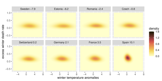
Figure S5: Excess Winter Death Rates: Fitted density surfaces for randomly selected countries obtained by the GSAW version of sliced Wasserstein regression with sliced Wasserstein fraction of variance explained at level 0.28.

REFERENCES

• Abeida et al. (2012) Abeida, H., Zhang, Q., Li, J., and Merabtine, N. (2012), “Iterative sparse asymptotic minimum variance based approaches for array processing,” IEEE Transactions on Signal Processing, 61, 933–944.
• Agranovsky and Quinto (1996) Agranovsky, M. L. and Quinto, E. T. (1996), “Injectivity sets for the Radon transform over circles and complete systems of radial functions,” Journal of Functional Analysis, 139, 383–414.
• Beylkin (1984) Beylkin, G. (1984), “The inversion problem and applications of the generalized Radon transform,” Communications on Pure and Applied Mathematics, 37, 579–599.
• Bigot et al. (2017) Bigot, J., Gouet, R., Klein, T., and López, A. (2017), “Geodesic PCA in the Wasserstein space by convex PCA,” Annales de l’Institut Henri Poincaré B: Probability and Statistics, 53, 1–26.
• Boissard et al. (2011) Boissard, E., Gouic, T. L., and Loubes, J.-M. (2011), “Distribution’s template estimate with Wasserstein metrics,” arXiv preprint arXiv:1111.5927.
• Bonneel et al. (2015) Bonneel, N., Rabin, J., Peyré, G., and Pfister, H. (2015), “Sliced and Radon Wasserstein barycenters of measures,” Journal of Mathematical Imaging and Vision, 51, 22–45.
• Bracewell (1956) Bracewell, R. N. (1956), “Strip integration in radio astronomy,” Australian Journal of Physics, 9, 198–217.
• Chen et al. (2020) Chen, Y., Dawson, M., and Müller, H.-G. (2020), “Rank dynamics for functional data,” Computational Statistics & Data Analysis, 149, 106963.
• Chen et al. (2021) Chen, Y., Lin, Z., and Müller, H.-G. (2021), “Wasserstein regression,” Journal of the American Statistical Association, 1–14.
• Chen and Müller (2022) Chen, Y. and Müller, H.-G. (2022), “Uniform convergence of local Fréchet regression with applications to locating extrema and time warping for metric space valued trajectories,” The Annals of Statistics, 50, 1573–1592.
• Courty et al. (2017) Courty, N., Flamary, R., Habrard, A., and Rakotomamonjy, A. (2017), “Joint distribution optimal transportation for domain adaptation,” Advances in Neural Information Processing Systems, 30.
• Cowling and Hall (1996) Cowling, A. and Hall, P. (1996), “On pseudodata methods for removing boundary effects in kernel density estimation,” Journal of the Royal Statistical Society: Series B (Methodological), 58, 551–563.
• Dai (2022) Dai, X. (2022), “Statistical inference on the Hilbert sphere with application to random densities,” Electronic Journal of Statistics, 16, 700–736.
• Deutsch (2012) Deutsch, F. (2012), Best Approximation in Inner Product Spaces, CMS Books in Mathematics, Springer New York.
• Ehrenpreis (2003) Ehrenpreis, L. (2003), The Universality of the Radon Transform, Oxford University Press.
• Epstein (2007) Epstein, C. L. (2007), Introduction to the Mathematics of Medical Imaging, SIAM.
• Fan and Müller (2021) Fan, J. and Müller, H.-G. (2021), “Conditional Wasserstein barycenters and interpolation/extrapolation of distributions,” arXiv preprint arXiv:2107.09218.
• Finch and Patch (2004) Finch, D. and Patch, S. K. (2004), “Determining a function from its mean values over a family of spheres,” SIAM Journal on Mathematical Analysis, 35, 1213–1240.
• Fowler et al. (2015) Fowler, T., Southgate, R. J., Waite, T., Harrell, R., Kovats, S., Bone, A., Doyle, Y., and Murray, V. (2015), “Excess winter deaths in Europe: A multi-country descriptive analysis,” The European Journal of Public Health, 25, 339–345.
• Ghosal et al. (2021) Ghosal, R., Varma, V. R., Volfson, D., Hillel, I., Urbanek, J., Hausdorff, J. M., Watts, A., and Zipunnikov, V. (2021), “Distributional data analysis via quantile functions and its application to modeling digital biomarkers of gait in Alzheimer’s Disease,” arXiv preprint arXiv:2102.10783.
• Gibbs and Su (2002) Gibbs, A. L. and Su, F. E. (2002), “On choosing and bounding probability metrics,” International Statistical Review, 70, 419–435.
• Guégan and Iacopini (2018) Guégan, D. and Iacopini, M. (2018), “Nonparametric forecasting of multivariate probability density functions,” University Ca’Foscari of Venice, Dept. of Economics Research Paper Series No, 15.
• Hazelton and Marshall (2009) Hazelton, M. L. and Marshall, J. C. (2009), “Linear boundary kernels for bivariate density estimation,” Statistics & Probability Letters, 79, 999–1003.
• Healy (2003) Healy, J. D. (2003), “Excess winter mortality in Europe: A cross country analysis identifying key risk factors,” Journal of Epidemiology & Community Health, 57, 784–789.
• Helgason (2010) Helgason, S. (2010), Integral Geometry and Radon Transforms, Springer New York.
• Herman (2009) Herman, G. T. (2009), Fundamentals of Computerized Tomography: Image Reconstruction from Projections, Springer Science & Business Media.
• Horbelt et al. (2002) Horbelt, S., Liebling, M., and Unser, M. (2002), “Discretization of the Radon transform and of its inverse by spline convolutions,” IEEE Transactions on medical imaging, 21, 363–376.
• Hron et al. (2020) Hron, K., Machalová, J., and Menafoglio, A. (2020), “Bivariate densities in Bayes spaces: Orthogonal decomposition and spline representation,” arXiv preprint arXiv:2012.12948.
• Hron et al. (2016) Hron, K., Menafoglio, A., Templ, M., Hruzova, K., and Filzmoser, P. (2016), “Simplicial principal component analysis for density functions in Bayes spaces,” Computational Statistics and Data Analysis, 94, 330–350.
• Kak and Slaney (2001) Kak, A. C. and Slaney, M. (2001), Principles of Computerized Tomographic Imaging, SIAM.
• Kantorovich (2006) Kantorovich, L. V. (2006), “On the translocation of masses,” Journal of Mathematical Sciences, 133, 1381–1382.
• Kolouri et al. (2019) Kolouri, S., Nadjahi, K., Simsekli, U., Badeau, R., and Rohde, G. (2019), “Generalized sliced Wasserstein distances,” Advances in Neural Information Processing Systems, 32.
• Kolouri et al. (2016) Kolouri, S., Zou, Y., and Rohde, G. K. (2016), “Sliced Wasserstein kernels for probability distributions,” in Proceedings of the IEEE Conference on Computer Vision and Pattern Recognition, pp. 5258–5267.
• Kuchment (2006) Kuchment, P. (2006), “Generalized transforms of Radon type and their applications,” in Proceedings of Symposia in Applied Mathematics, vol. 63, p. 67.
• Matabuena et al. (2021) Matabuena, M., Petersen, A., Vidal, J. C., and Gude, F. (2021), “Glucodensities: A new representation of glucose profiles using distributional data analysis,” Statistical Methods in Medical Research, 30, 1445–1464.
• Menafoglio et al. (2018) Menafoglio, A., Grasso, M., Secchi, P., and Colosimo, B. M. (2018), “Profile monitoring of probability density functions via simplicial functional PCA with application to image data,” Technometrics, 60, 497–510.
• Mersereau and Oppenheim (1974) Mersereau, R. M. and Oppenheim, A. V. (1974), “Digital reconstruction of multidimensional signals from their projections,” Proceedings of the IEEE, 62, 1319–1338.
• Meunier et al. (2022) Meunier, D., Pontil, M., and Ciliberto, C. (2022), “Distribution regression with sliced Wasserstein kernels,” arXiv preprint arXiv:2202.03926.
• Nadjahi et al. (2020) Nadjahi, K., Durmus, A., Chizat, L., Kolouri, S., Shahrampour, S., and Simsekli, U. (2020), “Statistical and topological properties of sliced probability divergences,” Advances in Neural Information Processing Systems, 33, 20802–20812.
• Nadjahi et al. (2019) Nadjahi, K., Durmus, A., Simsekli, U., and Badeau, R. (2019), “Asymptotic guarantees for learning generative models with the sliced-Wasserstein distance,” Advances in Neural Information Processing Systems, 32.
• Natterer (2001) Natterer, F. (2001), The Mathematics of Computerized Tomography, SIAM.
• Pegoraro and Beraha (2022) Pegoraro, M. and Beraha, M. (2022), “Projected statistical methods for distributional data on the real line with the Wasserstein metric.” Journal of Machine Learning Research, 23, 37–1.
• Petersen and Müller (2016) Petersen, A. and Müller, H.-G. (2016), “Functional data analysis for density functions by transformation to a Hilbert space,” The Annals of Statistics, 44, 183–218.
• Petersen and Müller (2019) Petersen, A. and Müller, H.-G. (2019), “Fréchet regression for random objects with Euclidean predictors,” The Annals of Statistics, 47, 691–719.
• Petersen et al. (2022) Petersen, A., Zhang, C., and Kokoszka, P. (2022), “Modeling probability density functions as data objects,” Econometrics and Statistics, 21, 159–178.
• Peyré et al. (2019) Peyré, G., Cuturi, M., et al. (2019), “Computational optimal transport: With applications to data science,” Foundations and Trends® in Machine Learning, 11, 355–607.
• Quellmalz et al. (2023) Quellmalz, M., Beinert, R., and Steidl, G. (2023), “Sliced optimal transport on the sphere,” arXiv preprint arXiv:2304.09092.
• Qureshi et al. (2005) Qureshi, S. A., Mirza, S. M., and Arif, M. (2005), “Inverse Radon transform-based image reconstruction using various frequency domain filters in parallel beam transmission tomography,” in 2005 Student Conference on Engineering Sciences and Technology, IEEE, pp. 1–8.
• Rabin et al. (2011) Rabin, J., Peyré, G., Delon, J., and Bernot, M. (2011), “Wasserstein barycenter and its application to texture mixing,” in International Conference on Scale Space and Variational Methods in Computer Vision, Springer, pp. 435–446.
• Radon (1917) Radon, J. (1917), “Über die Bestimmung von Funktionen durch ihre Integralwerte längs gewisser Mannigfaltigkeiten,” Akad. Wiss., 69, 262–277.
• Rustamov and Majumdar (2020) Rustamov, R. M. and Majumdar, S. (2020), “Intrinsic sliced Wasserstein distances for comparing collections of probability distributions on manifolds and graphs,” arXiv preprint arXiv:2010.15285.
• Shepp and Vardi (1982) Shepp, L. A. and Vardi, Y. (1982), “Maximum likelihood reconstruction for emission tomography,” IEEE Transactions on Medical Imaging, 1, 113–122.
• Tanguy et al. (2023) Tanguy, E., Flamary, R., and Delon, J. (2023), “Reconstructing discrete measures from projections. Consequences on the empirical sliced Wasserstein distance,” arXiv preprint arXiv:2304.12029.
• Vaart and Wellner (1996) Vaart, A. W. and Wellner, J. A. (1996), Weak Convergence and Empirical Processes, Springer.
• Villani (2003) Villani, C. (2003), Topics in Optimal Transportation, American Mathematical Society.
• Zhang et al. (2022) Zhang, Q., Li, B., and Xue, L. (2022), “Nonlinear sufficient dimension reduction for distribution-on-distribution regression,” arXiv preprint arXiv:2207.04613.
• Zhu and Müller (2023) Zhu, C. and Müller, H.-G. (2023), “Spherical autoregressive models, with application to distributional and compositional time series,” Journal of Econometrics.