DropCompute: simple and more robust distributed synchronous training via compute variance reduction

Abstract

Background. Distributed training is essential for large scale training of deep neural networks (DNNs). The dominant methods for large scale DNN training are synchronous (e.g. All-Reduce), but these require waiting for all workers in each step. Thus, these methods are limited by the delays caused by straggling workers.
Results. We study a typical scenario in which workers are straggling due to variability in compute time. We find an analytical relation between compute time properties and scalability limitations, caused by such straggling workers. With these findings, we propose a simple yet effective decentralized method to reduce the variation among workers and thus improve the robustness of synchronous training. This method can be integrated with the widely used All-Reduce. Our findings are validated on large-scale training tasks using 200 Gaudi Accelerators. A reference implementation is provided.

1 Introduction

Deep Neural Networks (DNNs) training continues to scale over size and computational footprint, as a result of a higher number of trainable parameters, wider and deeper models, and growing amounts of training data. As improvements in model quality (measured by test loss, for example) (Kaplan et al., 2020) lead over hardware capabilities (Hooker, 2020), this scale-up translates into a need for a growing number of training devices working in tandem (Chowdhery et al., 2022), turning distributed training to the standard approach for training DNNs on a large scale.

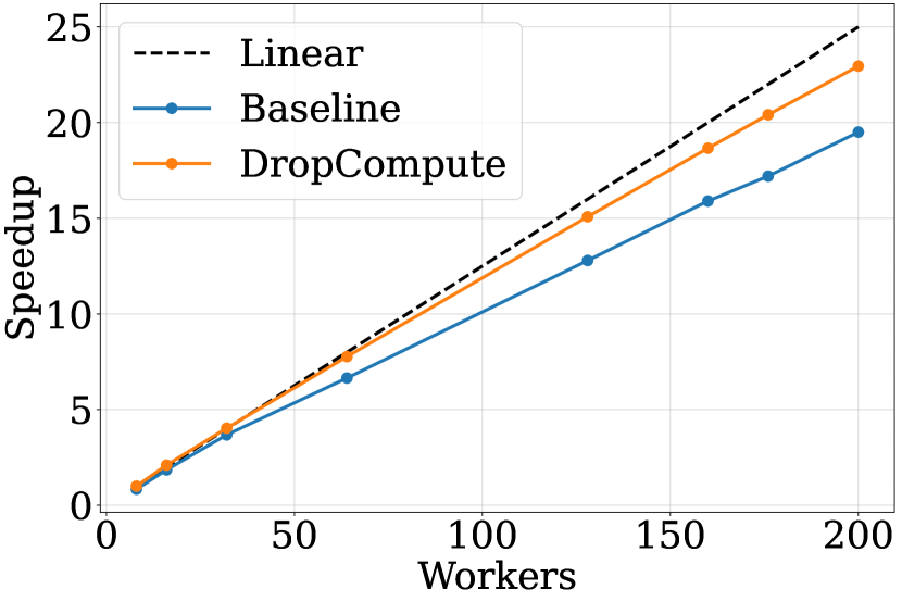
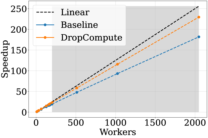
Figure 1: DropCompute improves robustness and scalability of synchronous training. A scale graph, showcasing the proposed method runtime performance of synchronous training of a 1.5 billion parameter model with additive noise, simulating compute variance. The baseline represents existing synchronous training and the dashed black line is linear scaling. (left) Real measurements of up to 200 workers. (right) An extrapolation to 2048 workers using a theoretical estimation, also proposed in the paper. More details are provided in section 5.2.

Distributed training typically refers to three parallelism paradigms — data parallel, model parallel and layer pipelining (Ben-Nun & Hoefler, 2019). Several variants and hybrid solutions exist in modern implementations such as tensor parallel (Narayanan et al., 2021) and parameter sharding (Rajbhandari et al., 2020; Rasley et al., 2020). These can be used separately or combined as they are orthogonal to each other. Mainly, data parallelism is straightforward, where the data is sharded among workers, and all workers share the same global model state. At each step, workers compute gradients locally and then aggregate them before taking an optimization step. When training synchronously, workers update their parameters in lockstep. This ensures that all workers hold a consensus on the same model and that gradients are averaged over all workers before being applied to the model. This approach is easy to implement and allows for good convergence properties, and correspondingly is the prevalent optimization method.

Although state-of-the-art models use synchronous optimization for training, synchronous methods scale poorly, as stragglers and communication overhead might severely deteriorate system utilization. Many resources are invested in alleviating these issues in large-scale training systems since even minor improvements can be worth hundreds of thousands of dollars. These issues are exacerbated as the required scale grows, even in homogeneous high-performance computing clusters (Petrini et al., 2003; Hoefler et al., 2010). In this paper, we are interested in cases where significant computing variance between the workers exists. This includes (but is not limited to) straggling workers.

For instance, certain learning tasks entail heterogeneity in the required computation of data, such as varying sentence lengths in language processing, or different image sizes and frame numbers in computer vision. In addition, recent state-of-the-art models use all three parallelism paradigms (data (DP), tensor (TP), and pipeline (PP) parallelism), thus each data parallel node is a set of processing units (accelerators) communicating between them (via TP and PP) to calculate the model gradients collectively. This could potentially intensify compute variance between data parallel workers. Moreover, sub-optimal hardware systems can also lead to straggling workers. Although some sources of heterogeneity can be mitigated by non-trivial engineering work, they still persist as challenges that can introduce compute variance and substantial performance drops. This is further discussed in appendix A.

In this paper, we suggest a simple, yet effective method called DropCompute to improve the robustness and scalability of synchronous optimization in the face of compute variance. We model the compute time as a random variable and show that under reasonable assumptions, a tail of straggling workers slows down the system at a rate that is not proportional to the contributed compute by these straggling workers. We harness the gradient accumulation method widely used in Large Language Models (LLMs) (Ott et al., 2018; Liu et al., 2019) to implement the method in a few lines of code on a relevant large-scale learning task.

The contributions of our work include:

• DropCompute: a novel, decentralized method to better handle heterogeneity or stragglers without additional hyper-parameters. DropCompute is hardware and framework agnostic, runs on top of existing optimizers, and can also be combined with other methods that improve other aspects of robustness such as communication overhead.

• A theoretical convergence proof of SGD with stochastic batch size, as in DropCompute.

• A theoretical runtime analysis on standard synchronous training and the proposed method. We find an approximation of the expected speedup using DropCompute, and show this speedup goes to infinity as the number of workers grows.

• An empirical evaluation of the proposed method on a relevant large scale task, using up to 200 accelerators connected with high bandwidth communication. For example, when using DropCompute before and after system optimizations (for both software and hardware) we show accelerations of 18% and 5%, respectively.

2 Related Work

The challenge of training deep neural networks on a large scale has been extensively explored. With rapidly growing models and data sizes, numerous works tackled the weaknesses in synchronous DNN training on a large scale and suggested methods to alleviate these weaknesses.

Redundancy methods. This line of work addresses the straggling worker problem using a redundancy mechanism. Redundant workers or redundant data are used such that straggling workers will not slow down the entire system (Chen et al., 2016; Bitar et al., 2020). These methods provide better robustness to synchronous training, even in the event of a complete failure of a subset of the workers or considerable communication slowdown. However, the robustness is limited by the redundancy factor, and more generally, more compute resources are required and full utilization cannot be achieved. In addition, some coordination method is required to keep the training synchronous, i.e., keeping consensus between the model replicas of the workers. In particular, Chen et al. (2016); Bitar et al. (2020) use a centralized approach of a parameter server to determine which workers are left out at each iteration. Modern large-scale systems use decentralized variants of All-Reduce (von Luxburg et al., ; Patarasuk & Yuan, 2009), so it is not trivial to determine which workers should be considered at each step, given that each worker can see a different subset of straggling workers. Moreover, combining redundancy with communication primitive collectives (e.g., All-Reduce) requires adaptation to existing underlying frameworks (Sanders et al., 2019).

Asynchronous optimization. Another approach is introducing asynchrony to the optimization. Asynchronous training is inherently more scalable than synchronous training by being robust to all kinds of workers and communication faults. This includes periodic synchronization by exchanging parameters every $\tau$ optimization steps (Stich, 2019; Lin et al., 2020; Wang & Joshi, 2021; Zhang et al., 2015; Wang et al., 2020; Li et al., 2020b, a), approximate distributed averaging where each worker communicates with a subset of workers each step (Jiang et al., 2017; Lian et al., 2017; Assran et al., 2019; Yang et al., 2020), and many more. These works provide better scale-up properties and improve time performance. The main drawback is asynchronous optimization itself. In practice, the convergence is less stable, and more optimization steps are needed to generalize as well as synchronous training. In addition, hyperparameters should be chosen more precisely to guarantee convergence and generalization properties (Giladi et al., 2019; Mitliagkas et al., 2016). Due to these issues, asynchronous methods are less commonly used on a large scale.

Sparse and compressed communication. Alternatively, several works addressed only the communication overhead. A common technique is to reduce the amount of data exchanged by the workers at each step. This can be done by gradient pruning (Xu et al., 2021), gradient compression (Seide et al., 2014; Chen et al., 2020; Tang et al., 2021) or low-rank approximation (Vogels et al., 2019). These works reduce the communication overhead in a deterministic form while ignoring any compute variance across processing workers. This makes these works orthogonal to ours and potentially can be combined with our method.

3 Reducing Compute Variance

This paper proposes a method called DropCompute that improves the robustness of synchronous training by reducing compute variance. First, we describe the vanilla synchronous training framework. Then, we introduce the proposed approach.

3.1 Problem setup

We start with a model formulation for data-parallel synchronous SGD training with $N$ workers, where each worker holds a replica of the model parameters $\theta$. In parallelism paradigms that combine TP or PP with DP, $N$ represents the count of data-parallel workers, not the total number of workers involved in training. Given a dataset $\mathcal{D}$, we are interested in minimizing the empirical loss

$$\mathcal{L}(\mathcal{D},\theta)=\frac{1}{\left|\mathcal{D}\right|}\sum_{z\in\mathcal{D}}\ell(z,\theta),$$

where $\ell(z,\theta)$ is the loss with respect to data-point $z$ and the model parameters $\theta$. At each step, the workers calculate gradients based on a local batch and then aggregate the gradients before taking an optimization step. An equivalent strategy would be that the workers aggregate the parameters after taking an optimization step based on the local gradients. The aggregation is done in a decentralized fashion, such as AllReduce.

We also consider the use of gradient accumulation to increase the size of the local batch. Gradient accumulation breaks down each worker’s local batch into $M$ micro-batches for computation, which enables reaching a large global batch size beyond hardware capacity. This is common practice in training of LLM on large scale where a substantial number of accumulations are being utilized (Smith et al., 2022; Nvidia, 2023). In each iteration $i$ and accumulation $m$, the gradients of the loss function with respect to the model parameters are computed, denoted by

$$g_{n}^{(m)}(\theta_{i})=\nabla\mathcal{L}(\mathcal{D}_{i,n}^{(m)},\theta_{i})\,,$$

where $\mathcal{D}_{i,n}^{(m)}\subseteq\mathcal{D}$ is the micro-batch $m$ of worker $n$, sampled without replacement from $\mathcal{D}$, and we assume a constant micro-batch size $|\mathcal{D}_{i,n}^{m}|$. The gradients accumulated by worker $n$ at step $i$ are

$$g_{n}(\theta_{i})=\frac{1}{M}\sum_{m=1}^{M}g_{n}^{(m)}(\theta_{i})\,.$$

Finally, the workers aggregate and average the computed gradients to update the model parameters

$$\theta_{i+1}=\theta_{i}-\eta g(\theta_{i});\quad g(\theta_{i})=\frac{1}{N}\sum_{n=1}^{N}g_{n}(\theta_{i})\,,$$ (1)

where $\eta$ is the learning rate. Equation 1 requires all workers to receive all gradients before updating the parameters. This communication restriction is what makes the training synchronous and ensures the model parameters are the same for all workers. However, due to this restriction, the slowest worker at each step dictates the iteration time. More generally, any variation in computation time among workers will lead to workers with idle time. Therefore, to improve the efficiency and robustness of the synchronous training process, we need to reduce the computation time variance among workers (namely, the compute variance).

3.2 Our method: DropCompute

To mitigate the effect of compute variance and to improve the robustness of synchronous training, we propose a simple yet effective method called DropCompute. DropCompute reduces the compute variance by introducing a compute threshold after which workers have to stop calculating local gradients and move directly to the communication phase, i.e., Equation 1.

In each iteration $i$, each worker $n$ measures the time while calculating its local batch, and compares it against a given threshold $\tau$, which is set as described in section 4.4. If that time exceeds the compute threshold, the worker stops and sends the gradients it has calculated so far. The rest of the training remains unchanged, thus synchronous training is intact. The pseudo-code of DropCompute is shown in Algorithm 1. This method maintains a decentralized approach while improving its robustness to compute variance and stragglers in particular. Since our method drops samples, the batch size is no longer deterministic. Specifically, the total batch size (the total number of samples used in one iteration by all workers) can be smaller than the maximal total batch size $b_{\max}=NM|\mathcal{D}_{i,n}^{(m)}|$. Nevertheless, we show both theoretically and empirically that this makes no difference to convergence or generalization when the number of computed samples remains the same. Next, we analyze this method in section 4 and evaluate it in section 5.

Algorithm 1 DropCompute on worker $n$ at iteration $i$

1:Input:  model parameters $\theta_{i}$; total number of micro-batches $M$; compute threshold $\tau$

2:     local batch data $\mathcal{D}_{i,n}=\{\mathcal{D}_{i,n}^{(1)},\mathcal{D}_{i,n}^{(2)},\cdots,\mathcal{D}_{i,n}^{(M)}\}$; step time $T_{n}$ to compute local batch $\mathcal{D}_{i,n}$

3:Initialize step time $T_{n}=0$ and accumulated gradients $g_{n}(\theta_{i})=0$

4:do (1) and (2) in parallel:

5:     (1) for $m=1,\dots,M$ do

6:              $g_{n}^{(m)}(\theta_{i})=\nabla\mathcal{L}(\mathcal{D}_{i,n}^{(m)},\theta_{i})$ $\triangleright$ Compute gradient

7:              $g_{n}(\theta_{i})\leftarrow g_{n}(\theta_{i})+g_{n}^{(m)}(\theta_{i})/M$ $\triangleright$ Accumulate gradients (atomic)      

8:     (2) wait for $T_{n}>\tau$ and break for loop (1)

9:Output: $g_{n}(\theta_{i})$ $\triangleright$ AllReduce

4 Method Analysis

After establishing the notion of compute variance and the formulation of the proposed method, we analyze synchronous training and the potential value of the proposed method on the training time performance. To do so, we start with convergence guarantees when using DropCompute. Then, we theoretically analyze the computation time with synchronous training and when using DropCompute. Through this analysis, we estimate the potential speedup over vanilla synchronous training.

4.1 Convergence analysis of DropCompute

Using DropCompute, the batch size is no longer fixed, but a random variable, which can also potentially depends on the data samples. To the best of our knowledge, this setting is somewhat different from existing convergence guarantees. Therefore, in this section, we provide convergence guarantees for DropCompute by analyzing the convergence of SGD with stochastic batch size.

Assumption 4.1.

Following the notations in section 3.1, consider a possibly non-convex smooth loss function $\mathcal{L}(\mathcal{D},\theta)$, with a global minimum $\theta^{*}\in{\mathbb{R}}^{d}$, and the following (commonly used) assumptions

1. L-smooth: All functions $\mathcal{L}(\cdot,\theta)$ are with L-Lipschitzian gradients.

2. Unbiased estimation: Each $\nabla\ell(z,\theta_{i}),z\in\mathcal{D}$ is an unbiased estimate of $\nabla\mathcal{L}(\mathcal{D},\theta_{i})$ which is the true (full batch) gradient at $\theta_{i}$. Namely, $\forall i:\mathbb{E}[\nabla\ell(z,\theta_{i})|\theta_{i}]=\nabla\mathcal{L}(\mathcal{D},\theta_{i})\,.$

3. Bounded variance: The variance of the stochastic gradient is bounded by a constant $\sigma$,

   $$\forall i:\mathbb{E}[\|\nabla\ell(z,\theta_{i})-\nabla\mathcal{L}(\mathcal{D},\theta_{i})\|^{2}|\theta_{i}]\leq\sigma^{2}\,.$$

Theorem 4.1.

Under the above assumption, applying SGD with DropCompute (Algorithm 1), ensures

$$\mathbb{E}\|\nabla\mathcal{L}(\mathcal{D},\bar{\theta})\|^{2}\leq\frac{2Lb_{\max}(\mathcal{L}(\mathcal{D},\theta_{1})-\mathcal{L}(\mathcal{D},\theta^{*}))}{K}+\frac{2\sigma\sqrt{L(\mathcal{L}(\mathcal{D},\theta_{1})-\mathcal{L}(\mathcal{D},\theta^{*}))}}{\sqrt{K}}~{},$$ (2)

where $b_{\max}$ is the maximal total batch size, $K$ is the total number of samples that are used throughout the training, $\theta_{1}$ is the initial model, and $\bar{\theta}$ is a random sample of $\theta_{i}$ from the trajectory obtained by Algorithm 1, where $i$ is selected with probability proportional to the total batch size at iteration $i$. The expectation is with respect to the randomization introduced due to sampling from $\mathcal{D}$ throughout the optimization process and with respect to choosing $\bar{\theta}$.

The bound in Theorem 4.1 is similar to existing fixed batch-size guarantees (Dekel et al., 2012). The second term in the bound does not degrade with the batch sizes, and behaves like $O(1/\sqrt{K})$, while the first term behaves like $O(b_{\max}/{K})$. This implies that as long as $b_{\max}\leq O(\sqrt{K})$, the second term is dominant and we are in the regime of linear speedup. This shows we can attain a linear speedup despite using changing batch sizes, as long as the maximal batch size is bounded.

Similarly, in Theorem D.1 in appendix D.1 we show that the loss itself converges, in the convex case along with a proof. The proof of Theorem 4.1 is provided in appendix D.2. Lastly, we discuss the impact of the stochastic batch size on generalization in appendix D.4.

4.2 Iteration time in standard synchronous distributed training

We start with finding a closed-form expression for the cumulative distribution function (CDF) of the iteration time, denoted as $T$, defined as

$$T=\max(T_{1},T_{2},...,T_{N})\,,$$

where $T_{n}$ represents the time taken by worker $n$ to compute its local batch, which follows some cumulative probability function $F_{T_{n}}(x)=\mathbb{P}(T_{n}<x),$ which we assume is independent for each worker. Let $F_{T}(x)$ represent the cumulative distribution function and $f_{T}(x)$ represent the probability density function of the maximum iteration time $T$. The relation between $F_{T}(x)$ and $F_{T_{n}}(x)$ is

$$F_{T}(x)=\mathbb{P}\left(\max\left(T_{1},\ldots,T_{N}\right)\leq x\right)=\prod_{n=1}^{N}F_{T_{n}}(x)\,.$$

Differentiating with respect to $x$ and applying the chain rule gives:

$$f_{T}(x)=\frac{dF_{T}}{dx}(x)=\sum_{n=1}^{N}f_{T_{n}}(x)\prod_{n^{\prime}\neq n}^{N}F_{T_{n^{\prime}}}(x)\,.$$

In the special case where all of the workers’ iteration time distributions are identically and independently distributed (i.i.d.), this reduces to the well-known formula:

$$f_{T}(x)=N\cdot f_{T_{n}}(x)\cdot F_{T_{n}}(x)^{N-1}$$ (3)

If the iteration time of each worker is distributed normally ($\sim\mathcal{N}(\mu,\sigma^{2})$), the expected value of $T$ can be approximated as shown by Bailey et al. (2014):

$$\mathbb{E}(T)\approx\sigma\cdot\left((1-\gamma)\cdot\Phi^{-1}\left(1-\frac{1}{N}\right)+\gamma\cdot\Phi^{-1}\left(1-\frac{1}{e\cdot N}\right)\right)+\mu$$ (4)

where $\Phi$ is the CDF of the standard normal distribution, and $\gamma$ is the euler-mascheroni constant. Asymptotically the total iteration time is $\mathbb{E}[T]=\Theta(\sqrt{\text{log}N})$. When the number of micro-batches $M\gg 1$, we can make a similar approximation under Central Limit Theorem (CLT) conditions. More details are in appendix C.2.

4.3 Iteration time and number of micro-batches with DropCompute

When using DropCompute with a constant threshold $\tau$, each worker is preempted at $\tilde{T}_{n}=\min\left\{\tau,T_{n}\right\}$ and joins the AllReduce. Therefore, the total iteration time with DropCompute is

$$\tilde{T}+T^{c}=\min\left\{\tau,T\right\}+T^{c}\,,$$

where $T^{c}$ is a serial latency present in each iteration, which includes the AllReduce step. This upper limit serves to clip extreme values of $T_{n}$, effectively constraining the range of potential outcomes for $\tilde{T}$. As a result, the compute time variability decreases, leading to a narrower distribution and enhanced compute efficiency. These effects are illustrated in Figure 2.

As a consequence of preempting each worker at $\tilde{T}_{n}$, the number of micro-batches computed in each step varies. Denote as $t_{n}^{(m)}$ the compute latency of a single micro-batch $m$ for worker $n$, and $T_{n}^{(m)}=\sum_{j=1}^{m}t_{n}^{(j)}$. We can define the average number of micro-batches computed by each worker before reaching threshold $\tau$ as

$$\tilde{M}=\frac{1}{N}\sum_{n=1}^{N}\sum_{m=1}^{M}\left\{\begin{array}[]{lr}1,&\text{if }T_{n}^{(m)}<\tau\\ 0,&\text{otherwise }\end{array}\right\}~{}.$$

Under CLT conditions, the expected value for $\tilde{M}$ can be approximated in a closed form:

$$\mathbb{E}[\tilde{M}]\approx\sum_{m=1}^{M}\Phi\left(\frac{\tau-m\cdot\mu}{\sqrt{m\cdot\sigma^{2}}}\right)$$ (5)

where $\mu,\sigma^{2}$ are the mean and variance for a single micro-batch $t_{n}^{(m)}$ compute latency, and $\Phi$ is the CDF of the standard normal distribution. This approximation closely fits the real value of $\tilde{M}$ and can be used to analyze the expected gain from DropCompute. More details in appendix C.2.

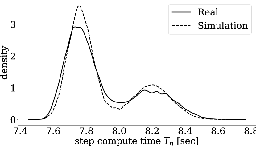
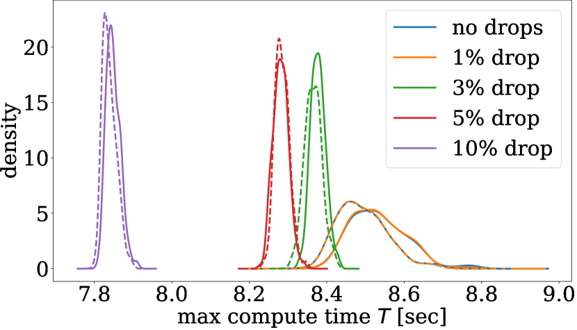
Figure 2: Reduction in variance and mean iteration time using DropCompute. Iteration time distribution of 200 workers using DropCompute on BERT 1.5B. (left) Step time $T_{n}$ distribution of all workers, without DropCompute. (right) Maximum iteration time $T$, across all workers, using DropCompute, with different drop rates. The dashed ‘simulation’ distribution is generated by drawing $T_{n}$ randomly from an independent normal distribution separately for each worker, using the empiric mean and variance of that worker.

4.4 Choosing the threshold

The throughput of the system can be seen as the number of micro-batches computed per second. For $N$ workers, this can be written as $NM/(T+T^{c})$. To evaluate the effectivness of DropCompute, we consider the difference in throughput between the baseline and when using DropCompute. Doing so, we can define the effective speedup for $\tau$ as:

$$S_{\mathrm{eff}}(\tau)=\frac{\text{DropCompute Throughput}}{\text{Baseline Throughput}}=\frac{N\tilde{M}/(\min\left\{\tau,T\right\}+T^{c})}{NM/(T+T^{c})}=\frac{\tilde{M}(T+T^{c})}{M(\min\left\{\tau,T\right\}+T^{c})}$$ (6)

Given the statistical characteristics of the training setting, it is possible to estimate analytically the expected value of the effective speedup $\mathbb{E}[S_{\mathrm{eff}}(\tau)]$ by using Equations 5 and 4. Moreover, when plugging in the asymptotic form of $\mathbb{E}[T]$, we find the expected speedup increases to infinity with $N$

$$\mathbb{E}[T]=\Theta(\sqrt{\text{log}N})\;\;\Rightarrow\;\;\mathbb{E}[S_{\mathrm{eff}}(\tau)](N)\underset{N\to\infty}{\longrightarrow}\infty$$

As shown in figure 3(b), Equation 4 is less accurate when samples deviate from a normal distribution.

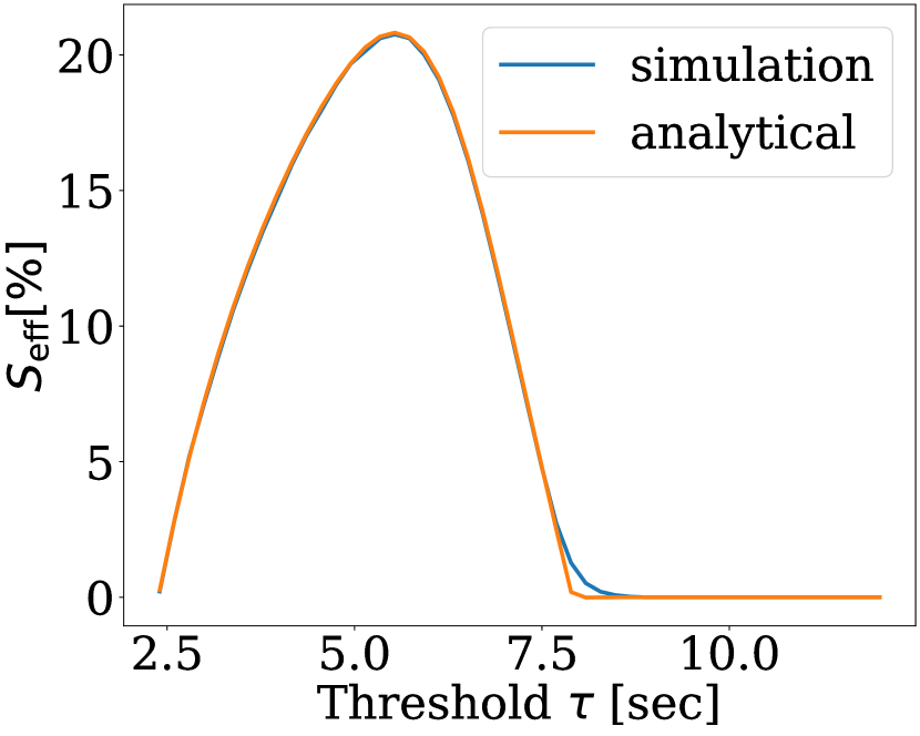
(a)

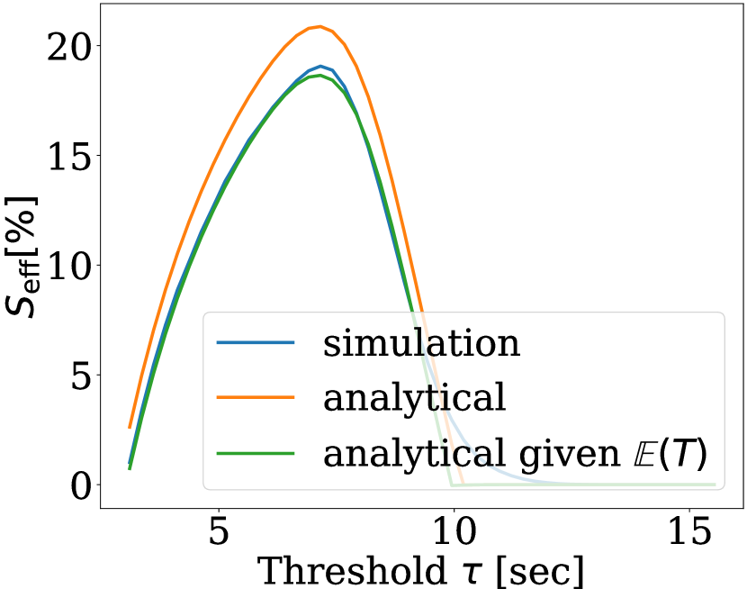
(b)

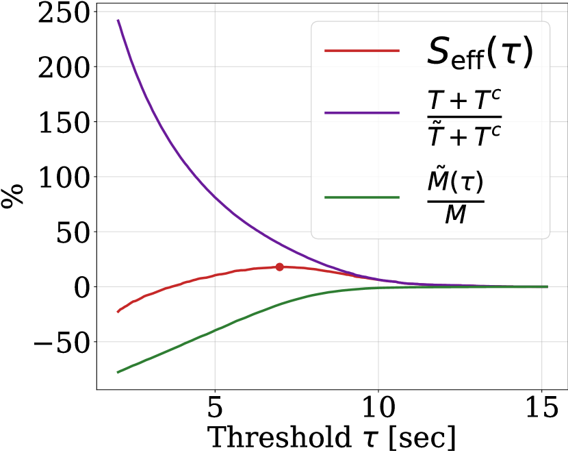
(c)

Figure 3: Statistical characteristics of the micro-batch computation latency $t_{n}^{(m)}$ can provide a reliable estimate of the effective speedup $S_{\mathrm{eff}}$. The graphs depict $S_{\mathrm{eff}}(\tau)$ based on Equation 6. Calculations rely on samples of $t_{n}^{(m)}$ to calculate $\tilde{M}$ and $T$, before plugging them into Equation 6. In the ‘simulation’ curves, we directly use the samples to calculate $\tilde{M}$ and $T$. For the ‘analytical’ curves, only the mean and variance of $t_{n}^{(m)}$ are used to approximate $\tilde{M}$ and $T$ using Equations 5 and 4, respectively. For ‘analytical given $\mathbb{E}[T]$’, $\tilde{M}$ is approximated using Equations 5, but $\mathbb{E}[T]$ is calculated directly from the samples. More details in appendix C.2. Panels: (a) The $t_{n}^{(m)}$ samples follow a normal distribution. (b) samples are taken from BERT1.5B pre-training with simulated delay as described in Section 5.2. (c) The optimal compute threshold can be found automatically. The effective speedup, micro-batch completion rate, and step speedup as a function of $\tau$ in a simulated delay environment.

To find the optimal compute threshold, we synchronize the empirical distribution of micro-batch compute latency between all workers after a few iterations. Given this distribution, we find $T$ and $\tilde{M}$, and search in a decentralized way for the threshold $\tau^{*}$ that maximizes the effective speedup $S_{\mathrm{eff}}(\tau)$ defined in Equation 6. Overall, the cost of synchronizing the empirical distribution and finding $\tau^{*}$ is negligible, compared to a full training session, because it happens only once in a training session. Lowering the threshold leads to reduced compute time but higher compute drop rates. Figure 3(c) highlights this trade-off and the optimal $\tau^{*}$ is marked.

4.5 Compensating for dropped samples

The effective speedup metric $S_{\mathrm{eff}}$, accounts for dropped samples by treating them as a source of slowdown in direct proportion to the drop rate. This consideration enables us to execute additional computations to achieve the theoretical speedup. The extent of extra time spent on redundant calculations can be as much as $R=(M/\tilde{M}-1)$ times the computational effort required when not applying DropCompute.

For instance, when 10% of the samples are dropped, we can expect to perform approximately 11% more calculations. Achieving this can be approached in several ways. One straightforward compensation method for LLM training involves adding an extra $R\cdot I_{\mathrm{base}}$ steps to the training process, where $I_{\mathrm{base}}$ represents the number of training steps conducted without using DropCompute. In practice, achieving the original accuracy often requires even fewer additional steps, as illustrated in Figure 5, resulting in an even higher effective speedup.

Another method of compensating for the dropped samples is to increase the maximal batch size. When increasing the batch by $R$ and dropping in average $1-\tilde{M}/M$, we keep the average batch size the same as without using DropCompute, hence compensating for the lost samples. A third method, orthogonal to the first two, is resampling dropped samples before starting a new epoch to diversify the overall samples seen by the model. These approaches are rigorously tested and compared in Table 1(b)

5 Experiments

To be useful, DropCompute must possess two properties. First, it should not compromise the accuracy of the trained model. This property is put to test in section 5.1 where we fully train BERT-Large and ResNet-50 (Devlin et al., 2018; He et al., 2015), each on a different task, with different drop rates to compare accuracy. Second, DropCompute should maintain a high level of runtime performance, especially when compute variance or straggling workers exist and vanilla synchronous training time deteriorates. Section 5.2 tests runtime performance of DropCompute by training a 1.5 billion parameter language model, BERT1.5B (Devlin et al., 2018) with additive noise to the compute time of each worker.

Experimental setup. The analysis of all BERT models is performed on the same dataset as Devlin et al. (2018), which is a concatenation of Wikipedia and BooksCorpus with 2.5B and 800M words respectively. The finetuning of the pretrained models is performed on SQuAD-v1 (Rajpurkar et al., 2016). We verify the generality of DropCompute by additional evaluation of a ResNet-50 model for image classification on ImageNet (Deng et al., 2009). The experiments depicted in section 5.2 and section 5.1 are executed on Habana Gaudi-1 and Gaudi-2 accelerators, respectively, with high performance network (Habana, 2020).

5.1 Generalization performance

The sole difference in the optimization when DropCompute is applied is that the batch size is not deterministic, but stochastic, as explained in section 3.2. To complement theorem 4.1, we examine the generalization performance achieved with a stochastic batch size on two popular tasks.

Image classification. To evaluate the generality of stochastic batch size and DropCompute in particular, we evaluate the Top-1 accuracy of a ResNet-50 model on the Imagenet dataset using our method. Since it is not common to use gradient accumulation in large scale training of this task, we simulate the drops such that each worker randomly drops its local batch, so the total batch size is stochastic. This simulated environment enables us to examine the extent of drop rate we can use without compromising accuracy. Figure 10 in appendix B.2.2 shows that up to $10\%$ drop rate, which is more than what DropCompute operates on, there is a negligible deterioration in accuracy.

(a) Varying drop rate, no compensation

% Drop rate	F1 score on dev set
0%	91.32 $\pm$ 0.15
2.5-3%	91.34 $\pm$ 0.04
5.5-6%	91.44 $\pm$ 0.02
10-11%	91.19 $\pm$ 0.02

(b) 10% drop rate, with compensation

Compensation method	F1 score on dev set
None	91.19 $\pm$ 0.02
11% extra steps	91.40 $\pm$ 0.08
11% increased batch size	91.38 $\pm$ 0.08
re-computation	91.19 $\pm$ 0.11

Table 1: Maintaining the accuracy of BERT-Large pretraining. Fine-tuning results on SqUAD v1.1, where the F1 score is obtained by the pretrained model. (a) The effect of different drop rates during pretraining on the final accuracy, without compensating for the dropped samples. (b) When 10% drop rate is used during pretraining, with different methods of compensating for the dropped samples.

Large language model. Training LLMs is resource intensive, typically using large batch sizes, which makes DropCompute appealing. We evaluate DropCompute method on this task by fully pretraining BERT-Large model several times, each with a different drop rate. We follow the optimization regime described in You et al. (2019) with a batch size of 64K for phase-1 and 32K for phase-2 (more details are provided in appendix B.2). Each of the pretrained models is fine-tuned on the SQuAD task 3 times with different initializations. Fine-tuning is performed without drops, as it is not a large scale resource consuming task. Table 1(a) shows the average accuracy ($\pm$ standard deviation) obtained for each drop rate. As shown, DropCompute at drop rates of up to $10\%$ have negligible accuracy difference. Higher values measured up to $20\%$ of dropped gradients provide acceleration with a small yet discernible hit on accuracy. We note that these results are for a fixed budget of steps. In the presence of compute variance, the effective speedup indicates that additional steps can be executed while still maintaining competitive runtime performance. This notion is demonstrated in section 5.2.

5.2 Runtime performance

The main purpose of our proposed method is to maintain runtime performance when compute variance is present. We examine this by measuring the speedup of DropCompute over standard synchronous training in several settings. First, we measure the potential speedup for different drop rates and training settings by post analysis of synchronous training without drops. In addition, we introduce compute variance by training with additive noise, and measure actual speedups using DropCompute. The experiments in this section are performed on BERT1.5B. Details are provided in appendix B.1.

Training with different number of workers and micro-batches. We evaluate the potential speedup of DropCompute on several training settings with natural heterogeneity and no drops. For each setting, we post analyze what would have been the speedup for different drop rates. As can be seen in Figure 4, DropCompute exhibits increasing benefits with a growing number of workers and compute requirements. However, there are diminishing returns in terms of speedup with more accumulations. This could possibly be explained by the amortization time of a large number of micro-batches.

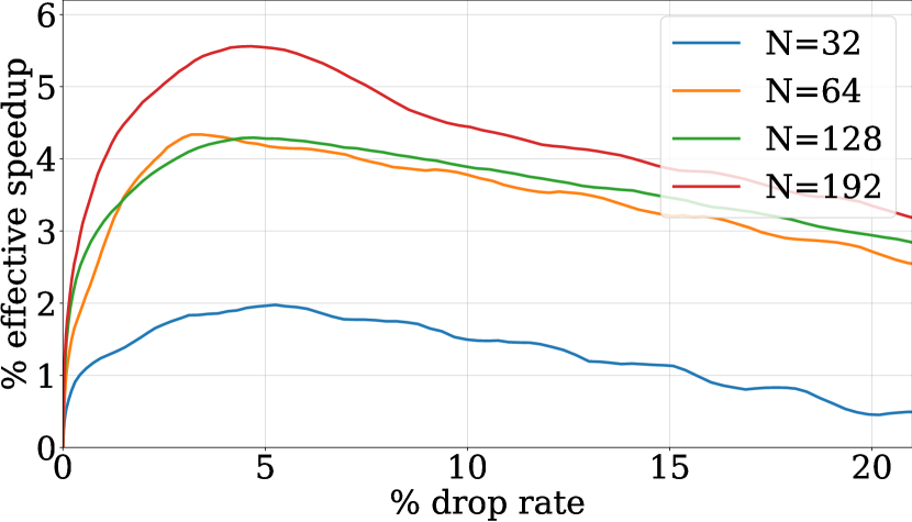
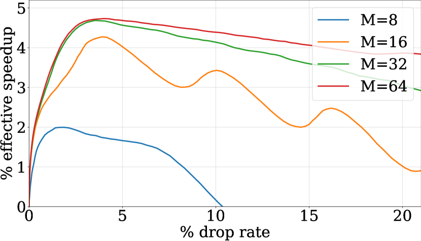
Figure 4: DropCompute exhibits increasing benefit on a large scale. Effective speedup versus drop rate with (left) 32 accumulations and varying workers, and (right) 112 workers and varying number of accumulations.

Simulated delay environment. Although DropCompute may have value when the workers’ compute latency variance is low, its significance becomes crucial when the workers’ compute latency exhibits high variability. To evaluate our method, we introduce a delay environment where random latency is added to each micro-batch computation. This additive noise follows a bounded log-normal distribution. Detailed information and motivation regarding the additive noise are in appendix B.1. The experiments are executed with 12 gradient accumulations and a local batch size of 192. In Figure 1, the negative impact of compute variance on scalability is demonstrated and mitigated using DropCompute. The results in Figure 1 also correspond to section 4 and Equation 11, where a theoretical extrapolation follows the same trend line. When utilizing DropCompute in this setup, achieving the same training loss as the baseline might requires additional training steps, however, it leads to a notable reduction in overall training time. Figure 5 demonstrates it in a training session with 64 workers, where approximately 3% more steps is needed to reach the same loss, in 13% less time.

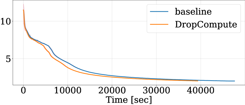
Figure 5: DropCompute improves training time for workers with compute variance. Train loss curve of BERT1.5B pretraining, in a simulated delay environment. (left) Horizontal axis in training steps, and (right) horizontal axis in training time.

6 Discussion

Summary. Efficient scalable systems are a key component to enable the continued development of deep learning models. To this day, state-of-the-art models rely on synchronous distributed optimization. The challenge to maintain synchronous training as an efficient solution grows larger with the quickly growing model sizes and data. Therefore, improving the robustness and scalability of distributed synchronous training is an important endeavor. This paper tackles the challenge of maintaining synchronous training scalable in the face of compute variance. We propose DropCompute to improve the robustness of synchronous training. Workers drop their remaining compute when they reach a compute threshold, determined by exchanging and analyzing the compute latency distribution. We find that for a small percentage of dropped data, a much larger percentage of time can be saved, depending on the compute latency distribution of the workers. In addition, we provide theoretical convergence guarantees and runtime predictions. We further discuss the motivation behind DropCompute and how it effectively solves the problem in appendix A.

Limitations. While DropCompute is simple and straightforward, it deals with system efficiency, and as such, the user-level implementation provided is not optimal. Mainly, the provided implementation is limited by using many gradient accumulations and integrating compute timeout in between them. However, we believe that this is not a major concern since having multiple gradient accumulations is a common practice in training LLM on a large scale and is used in state-of-the-art training configurations (Smith et al., 2022; Nvidia, 2023). In addition, DropCompute addresses variance that originates from the compute stage of the training iteration and does not solve the potential issue of network variance during the all-reduce stage.

Future directions. DropCompute is described and analyzed in this paper as a method built on top of synchronous training. However, this method can be integrated with other possibly asynchronous methods such as periodic synchronization. In appendix B.3, we implement DropCompute on top of Local-SGD (Lin et al., 2020) and show that DropCompute can also improve the robustness of Local-SGD to stragglers. A different extension for DropCompute is to apply it during the model backward calculation and save the partial gradients that were already calculated. This would generalize DropCompute for workloads that do not utilize gradient accumulations. However, it will require further study as it differs from the stochastic batch-size setting where the entire data sample is either saved or dropped.

Appendix

Appendix A Further discussion

In this section, we will further elaborate on the motivation for using DropCompute and how it mitigates existing problems in large-scale training.

A.1 Motivation

The primary objective of DropCompute lies in the mitigation of compute latency variance among workers. This raises the question of the significance of compute variance in the context of our research. Compute variance can arise from various sources, including but not limited to faulty hardware, clock throttling, host preemption/overhead, inefficient load balancing, connectivity issues (particularly in model parallel settings), and more. Inefficient load balancing is especially in particular, when dealing with with dynamic sentence/image sizes (Tan & Le, 2021; Dehghani et al., 2023; Raffel et al., 2020b) because it requires special treatment for each model and data set, often at the expense of performing redundant work. Addressing these issues typically requires intricate engineering efforts:

• Regular testing and replacement of faulty hardware.

• Mitigation of host overhead through the implementation of latency-hiding techniques and script optimization.

• Management of inefficient load balancing on a per-workload basis, employing strategies such as sample padding and packing.

However, it is essential to recognize that each of these issues represents a potential single point of failure. The triggering of any one of them can result in a substantial performance degradation within large-scale systems. Some of our early experiments exhibited naturally such sub-optimal behavior where we clearly see a large variance in compute latency between iterations and workers (as shown in figure 6). As our goal is to improve robustness (i.e. performance for outlier cases), these cases are important. Moreover, after the compute variance was reduced by HW and SW optimizations, we were still left with some compute variance (as shown in figure 2).

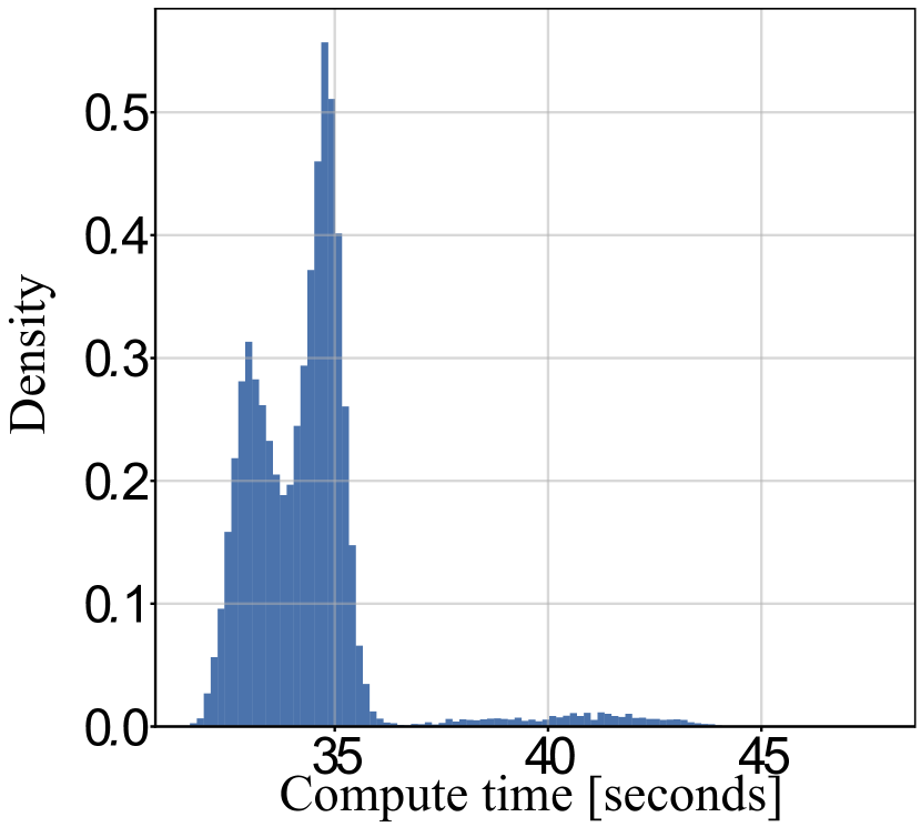
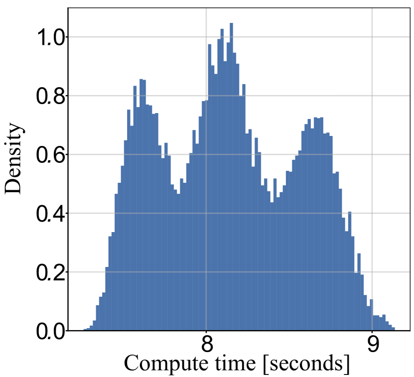
Figure 6: Single iteration latency histogram in a sub-optimal system. These histogram were recorded in BERT1.5B training, before optimizing our system. (left) Training with 162 workers and 64 gradient accumulations. When applying DropCompute in this setting, we achieved $\sim 18\%$ performance boost. (right) Training with 190 workers and 16 gradient accumulations.

These examples lead us to the conclusion that, in practice, workers do not finish computation at the same time, and this can have a significant impact on the training speed. Moreover, the effect of stragglers and compute variance on the training speed is expected to get worse as the distributed scale increases. This is due to the maximal worker distribution relation stated in equation 3. When modeling the additive latency as normally distributed, the average maximal worker latency, $\mathbb{E}[T]$, increases with the number of workers $N$ as $\mathbb{E}[T]=\Theta(\sqrt{\text{log}N})$ as shown in appendix C.2.

A.2 Effectiveness

Mitigating slowdowns resulting from compute variance can be achieved easily buy using DropCompute. For instance, in a sub-optimal system with stragglers, as illustrated in Figure 6 (left), we were able to recover approximately 18% of the runtime performance. The contribution of DropCompute can be even more significant in different systems with varying noise distributions, as demonstrated in Appendix C.3.

Furthermore, even when assuming a normal distribution of noise, theoretical analysis indicates a substantial speedup as the number of workers $N$ increases: $S_{\mathrm{eff}}(N)\underset{N\to\infty}{\longrightarrow}\infty$. On the tested system, after reducing compute variance through hardware and software optimizations, we achieved a 5% performance boost with 196 workers (see Figure 2). Notably, this speedup continues to increase as the scale of the system grows. These examples underscore how DropCompute enhances the robustness of large-scale training, effectively recovering lost performance attributed to stochastic performance outliers.

Lastly, it’s important to emphasize that even a modest improvement in large-scale training performance can yield significant cost savings. For example, assuming a cost of $10–32/hour/8xA100 (according to AWS pricing), saving 5% of the training time for a 176B model, such as (Scao et al., 2022), would result in savings ranging from $67,686 to $216,598. For longer-trained models, like (Touvron et al., 2023), the savings could reach $107.50 to $344,064."

Appendix B Experiments

B.1 Runtime performance experiments

In this section, we provide details for the experiments of section 5.2.

Experiment details. As mentioned in the paper in section 5.2, we pre-train BERT1.5B following Habana (2023). The experiments in this section use up to 200 Gaudi accelerators with high bandwidth inter-connectivity. The training is done with a maximum input sequence length of 128 and 80 maximum predictions per sequence. The training regime consists of a local batch size of 196, 12 gradient accumulations, LANS optimizer (Zheng et al., 2020), and a learning rate of 0.0015. Due to the large capacity of the model, we used ZeRO optimizer stage 1 to fit the model in memory (Rajbhandari et al., 2020).

Simulated delay. Many frameworks use padding to allow for constant input length which improves hardware efficiency (Kosec et al., 2021). However, some learning tasks inherently involve dynamic shapes, such as translation (Ott et al., 2018) and multi-task sequences (Raffel et al., 2020a). These use cases motivate us to explore scenarios of dynamic length via simulation. To demonstrate the value of DropCompute in dealing with compute variance we added to each micro-batch compute time an additional random waiting time. The additive noise is based on a Log-normal distribution since it is typical for user post lengths in internet discussions (Sobkowicz et al., 2013), which are used as training data in recent language models (Radford et al., 2019). To make this setting more realistic, we scale down and bound the noise so that each accumulation takes $\times 1.5$ longer on average, and, in extreme cases, can take up to 6 times longer. This allows us to simulate stragglers and high compute variance while keeping a conservative limit on iteration time. Thus, the additive noise takes the form of

$$\epsilon=\min\left(\frac{1}{\alpha}Z,\beta\right),\;\;\;\;\;\;\;\;\;Z\sim\mathrm{LogNormal}(4,1)\,.$$

This noise was added to each accumulation

$$t_{n}^{(m)}\leftarrow t_{n}^{(m)}+\mu\cdot\epsilon\,,$$

where $\mu$ is the mean value for $t_{n}^{(m)}$, $\alpha=2\exp(4.5)$ and $\beta=5.5$ are the scaling and bounding constants, and the log-normal parameters (4,1) fit user post lengths, as seen in Sobkowicz et al. (2013). As illustrated in Figure 7, the noise distribution leads to each micro-batch latency increased by up to $6\mu$, while the majority of accumulations have low latency. Further analysis on the effect of noise properties is discussed in C.3.

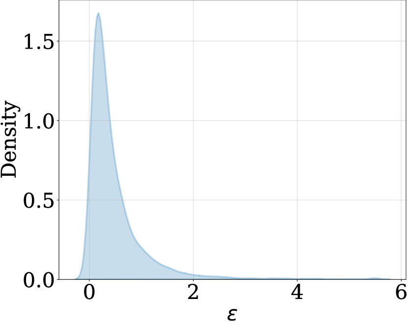
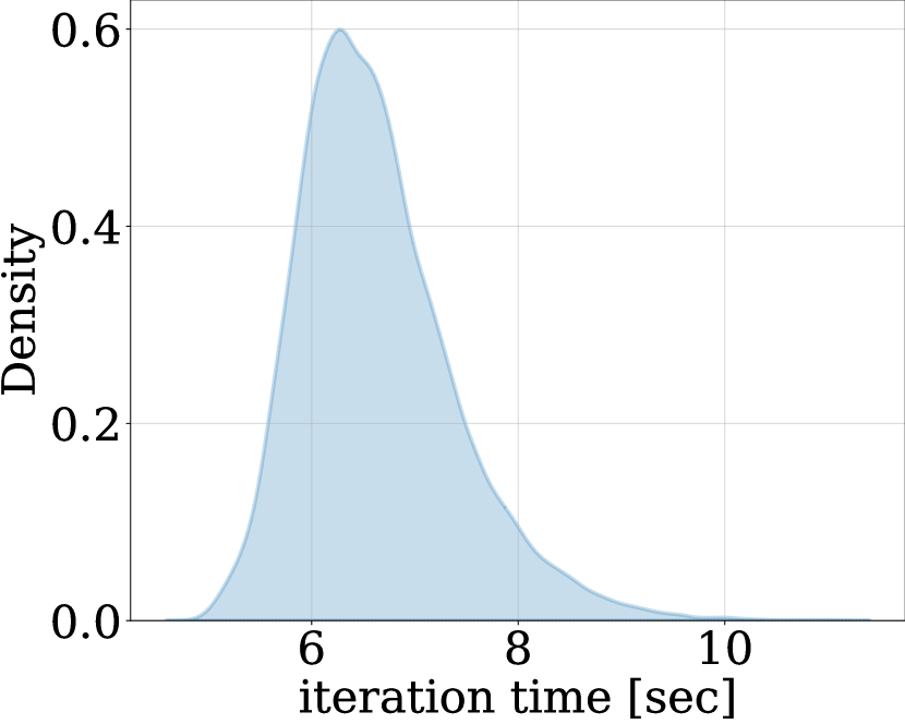
Figure 7: The latency distribution in a simulated delay environment. (left) The distribution of the additive noise $\epsilon$, added to each accumulation. (right) The distribution for iteration time $T_{n}$, with 12 accumulations, each with added noise, in BERT1.5B training.

B.2 Generalization experiments

In this section, we provide details for the experiments of section 5.1.

B.2.1 Large language models

Here we provide more details about how the LLM experiment was executed as well as additional graphs related to the LLM experiment described in section 5.1.

Experiment details. As mentioned in the paper, in section5.1 we follow You et al. (2019) optimization regime with LAMB optimizer. Specifically, for phase-1 where the sequence length is 128 tokens per sample, we use a batch size of 64K, the learning rate is 0.006, the warmup ratio is 0.2843, and the steps number is 7038. For phase-2 where the sequence length is 512, we use a batch size of 32K, the learning rate is 0.004, the warmup ratio is 0.128 and the steps number is 1563. The experiments were executed on 64 workers.

Batch size distribution. As explained in section 5.1 we fully pretrain a BERT-Large model with DropCompute several times, each with a different drop rate. Figure 8 shows the empirical batch distribution of each of the drop rates in phase-1.

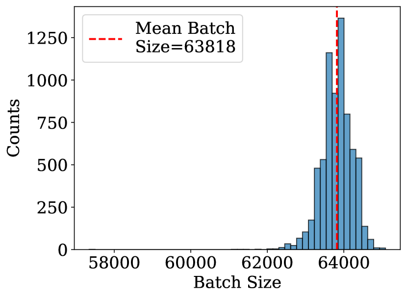
(a)

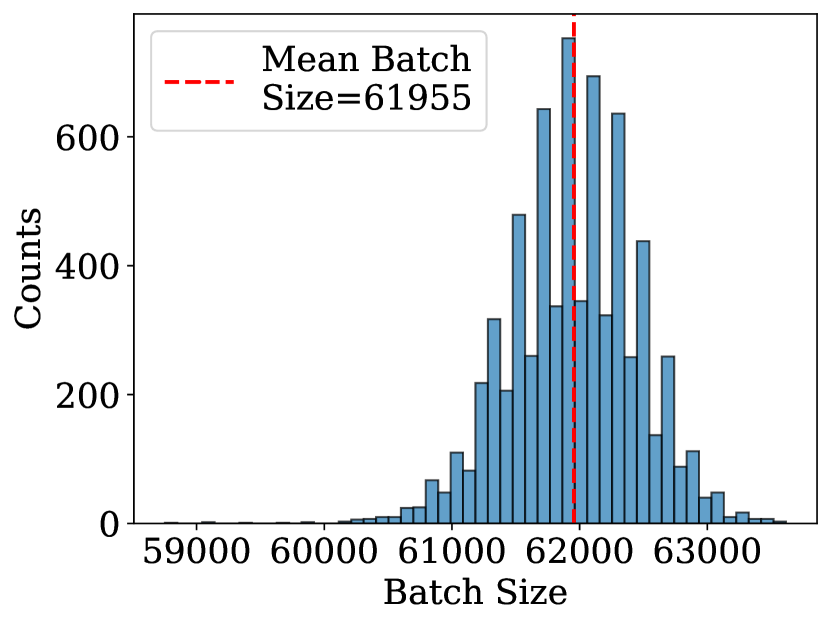
(b)

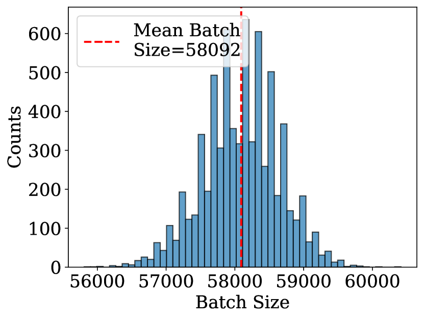
(c)

Figure 8: Batch size distribution. BERT-Large phase-1 pretraining batch size distribution when using DropCompute and drop rate of (a) 2.5% , (b) 5.5%, and (c) 11.5%

Convergence loss. In addition to the results depicted in Table 1(a), we show the convergence of the training loss with the different drop rates in Figure 9.

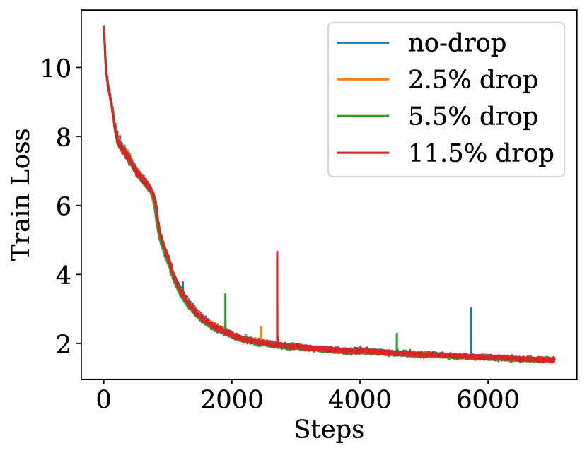
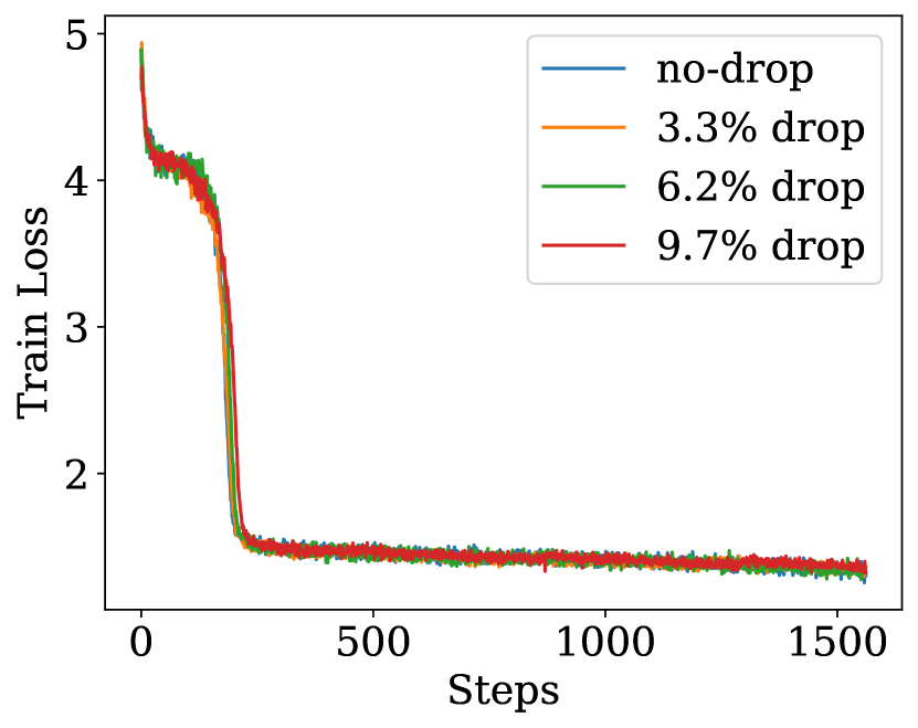
Figure 9: Train loss convergence. BERT-Large phase-1 (left) and phase-2 (right) pretraining train loss for different drop rates.

B.2.2 Image classification

This section provides the details of the image classification experiment described in section 5.1 as well as Figure 10 which is referenced from the paper.

Experiment details. To simulate DropCompute, at each training step, the gradients of each worker are set to zero with a probability of $P_{\text{drop }}$. We repeat each training process 3 times with different initializations. To examine the generalization of DropCompute over different optimizers, we implement our method on two popular training regimes of ResNet50. First, we follow the optimization regime described in Goyal et al. (2017) that uses SGD with 32 workers and a global batch size of 4096. Second, we follow Mattson et al. (2019) that uses LARS (You et al., 2017) with 8 workers and a global batch size of 2048.

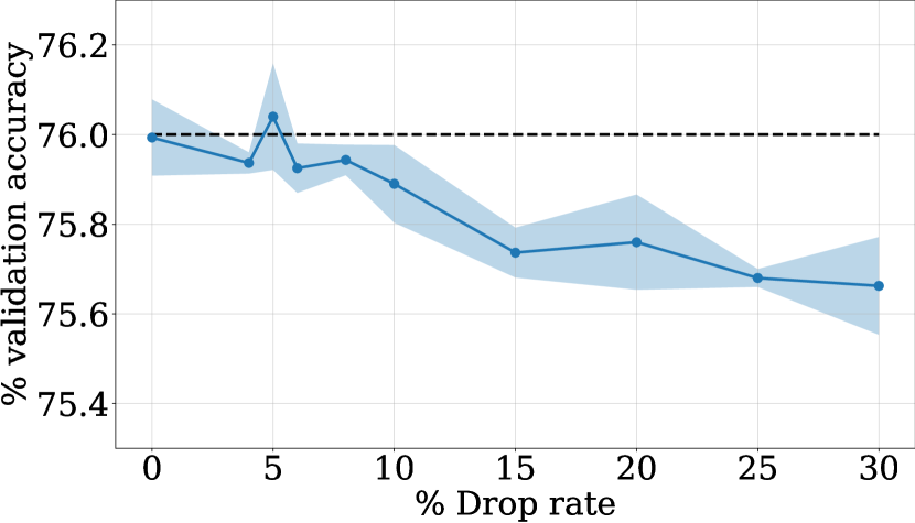
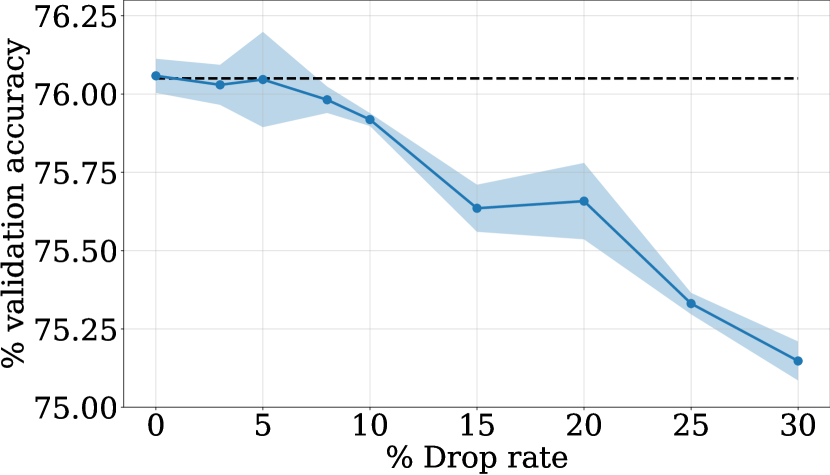
Figure 10: Generalization over varying drop rates. Top-1 validation accuracy of ResNet50 trained on ImageNet with varying simulated drop rates. The dashed line is the baseline accuracy without drops. The solid line is the average over 3 runs, and the blue area is the standard deviation. (left) Training regime with SGD (Goyal et al., 2017). (right) Training regime with LARS (Mattson et al., 2019). Up to a 10% drop rate, there is a negligible accuracy deterioration.

Learning rate correction. Previous works showed that the learning rate should be scaled with respect to the batch size (Hoffer et al., 2017; Goyal et al., 2017). With a stochastic batch size and specifically DropCompute, it is possible that a learning rate correction should be considered to maintain accuracy with the same number of steps. We examine such corrections when training with stochastic batch size. First, we decrease the learning rate by a constant factor, equal to the average drop rate. Specifically, for an average drop rate $P_{\text{drop}}\in[0,1]$ we multiply the learning rate by $(1-P_{\text{drop}})$. A different correction we consider is a stochastic correction, such that in each step we divide the gradients by the computed batch size, instead of the original batch size. This result in a different normalization in each step depending on the actual dropped samples. We note that for the latter, the workers have to synchronize the computed batch of each worker at each step. This is generally can be done during the AllReduce, with negligible overhead. We repeat the training of ResNet50 on ImageNet as described in Goyal et al. (2017) to evaluate the generalization without correction and with the two suggested corrections. We use 128 workers, batch size 8192, and use ghost batch norm (GBN) (Hoffer et al., 2017) to match batch normalization of 32 samples and restore the results in Goyal et al. (2017). As can be seen in Figure 11, for low drop rates, there is no superior correction method, and no correction generally achieves the same generalization. Yet, it is possible that a learning rate correction could potentially improve generalization on a different task or with a different optimizer.

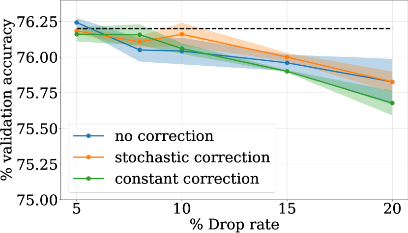
Figure 11: Learning rate correction is not necessary for low drop rates. Top-1 validation accuracy of ResNet50 trained on ImageNet with varying simulated drop rates, using the learning-rate correction methods described in B.2.2. The dashed line is the baseline accuracy without drops. Each solid line is the average over 3 runs, and the area around it is the standard deviation. Up to a 10% drop rate, there is a negligible accuracy deterioration regardless of the correction applied.

B.3 Local-SGD

Periodic synchronization methods, such as Local-SGD, provide better scalability properties than synchronous methods. By exchanging parameters less frequently, communication overhead is mitigated. For compute variance and straggling workers in particular, the robustness of these methods greatly depends on the distribution of the compute time between workers. For example, when straggling workers appear randomly with homogeneous distribution, Local-SGD can mitigate the straggling workers slowdowns to some extent; this is because of the amortization effect in synchronizing periodically once every several steps. On the other hand, if straggling workers appear from a small set of workers such as a single server, a realistic scenario, Local-SGD acts more closely to synchronous training as the worst-case scenario is when a single worker always straggling behind. DropCompute can be easily integrated with Local-SGD by leveraging periodic synchronization instead of gradient accumulations. We implement DropCompute on top of Local-SGD by comparing the compute time with a threshold at each local step. We show that when stragglers are apparent, DropCompute can improve the robustness of Local-SGD. We randomly slow down workers to simulate stragglers in two scenarios as described in Figure 12. The experiment setting is 32 workers training on ResNet50 and ImageNet. At each local step, each worker is selected to be straggler with a $4\%$ chance. This way, there is at least 1 straggler for each local step on average. We measure relative speedup compared to synchronous training in terms of step time, both for Local-SGD and with DropCompute on top of Local-SGD. As can be seen, with DropCompute (set to $~{}6.2\%$ drop rate in this experiment) we improve the robustness of Local-SGD.

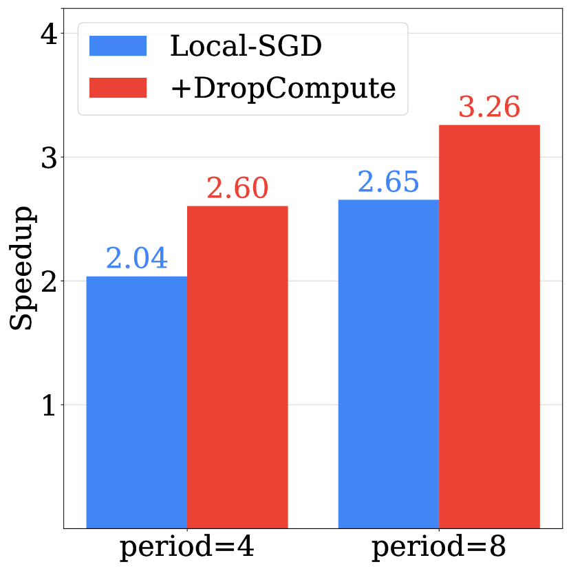
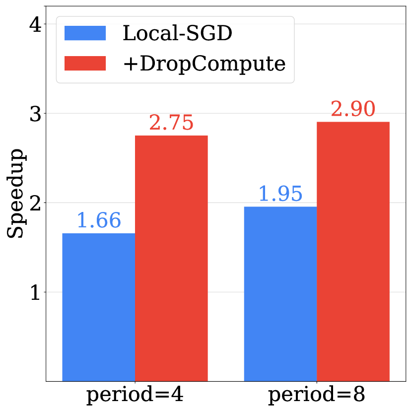
Figure 12: DropCompute can be integrated with Local-SGD to improve robustness. Speedup of each method compared to synchronous training in a straggling workers environment. In each local step workers are randomly drawn to be stragglers. If selected as a straggler, the worker waits 1 second before continuing. The synchronization period of Local-SGD is denoted in the x-axis. (left) Uniform stragglers. (right) Single server stragglers.

Appendix C Analyzing the effective speedup using DropCompute

In this section, we provide more details on the process of choosing the threshold $\tau^{*}$ that will maximize the effective speedup. We begin by giving technical details on the process used during training, given samples drawn from the empirical distribution of the compute latency. Next, we continue to explore and establish the analytic connection between the latency statistics and the effective speedup.

C.1 Automatic selection of the drop threshold

In Algorithm 2 below we present the algorithm used for automatic selection of the drop threshold $\tau$. In this algorithm, $t_{i,n}^{(m)}$ is the time it takes worker $n$ to process micro-batch $m$ at step $i$ and $T_{i}^{c}$ is the time spent on communication for at step $i$. This data is measured by each worker, and then synchronized between all workers after $I$ iterations. After the synchronization step each worker will have the same drop threshold $\tau$, which depends on both his own speed and the compute latency of the other workers. Since $T_{i}^{c}$ is used in the normalization of the effective speedup, the chosen threshold takes into account both compute and communication time.

Algorithm 2 Automatic choice for the optimal threshold $\tau$

Input:

number of workers $N$

number of iterations $I$

number of micro-batches per step $M$

micro-batch time samples $\{\{t\}_{i,n}^{(m)}\}^{i\in[1:I],n\in[1:N],m\in[1:M]}$

communication time for each iteration $T_{i}^{c}$

potential thresholds $[\tau_{0},\tau_{1},...]$

for $\tau\in[\tau_{0},\tau_{1},...]$ do

     for $i=1$ to $I$ do

         Initialize completed micro-batch count: $\tilde{M}_{i}(\tau)=0$

         Initialize compute step latency for all workers: $T_{i}=0$

         for $n=1$ to $N$ do

              Initialize single worker step compute latency: $T_{i,n}=0$

              for $m=1$ to $M$ do

                  $T_{i,n}\leftarrow T_{i,n}+t_{i,n}^{(m)}$

                  $\tilde{M}_{i}(\tau)\leftarrow\tilde{M}_{i}(\tau)+\frac{1}{N}\cdot\left\{\begin{array}[]{lr}1,&\text{if }T_{i,n}<\tau\\ 0,&\text{otherwise }\end{array}\right\}$               

              $T_{i}\leftarrow\text{max}(T_{i},T_{i,n})$ $\triangleright$ compute time of the slowest worker at step (i)          

         $S_{i}(\tau)=\frac{T_{i}+T_{i}^{c}}{\min(\tau,T_{i})+T_{i}^{c}}\cdot\frac{\tilde{M}_{i}(\tau)}{M}$ $\triangleright$ Effective speedup for step (i)      

     $S_{\mathrm{eff}}(\tau)=\frac{1}{I}\sum_{i=1}^{I}{S_{i}(\tau)}$ $\triangleright$ Mean speedup for threshold ($\tau$)

$\tau^{*}\leftarrow\text{argmax}_{\tau}\left(S_{\mathrm{eff}}(\tau)\right)$

C.2 DropCompute speedup analytic analysis

In this section we further explore the relation between the compute latency distribution and the effective speedup. We will derive a closed-form representation of the effective speedup by making certain assumptions. First we assume that

Assumption C.1.

$t_{n}^{(m)}$ is i.i.d with finite mean $\mu$ and finite variance $\sigma^{2}$.

Note that in the assumption above, for simplicity of presentation we assumed all workers as identical and so $\mu$ and $\sigma^{2}$ are identical. However, it is possible to derive similar properties with nonidentical workers, each with their own $\mu_{n}$, $\sigma_{n}$. Next, denote the time for completion of micro-batch $m$ as $T_{n}^{(m)}=\sum_{j=1}^{m}t_{n}^{(j)}$. Then, we assume

Assumption C.2.

$T_{n}^{(m)}\text{ is Gaussian }\sim\mathcal{N}(m\mu,m\sigma^{2})$ for $m>\sqrt{M}\,.$

This assumption holds in the limit $M\to\infty$ given Assumption C.1, from the Central Limit Theorem (CLT). Lastly, denoting $\tau$ as the threshold used, we assume

Assumption C.3.

$\tau>\frac{M\mu}{2}\,.$

This bound can be considered as the minimum threshold allowed, in order for DropCompute to be effective. Taking a lower threshold will result in unacceptable high drop rate.

Using these assumptions we first derive analytical expression for the iteration time $\mathbb{E}[T]$ and the mean completed number of gradient accumulations $\mathbb{E}[\tilde{M}]$ with DropCompute. Then, we combine these expressions to obtain an expression for the mean effective speed $\mathbb{E}[S_{\mathrm{eff}}]$.

Figure 3(b) shows an example of how close is the derived expression of $\mathbb{E}[S_{\mathrm{eff}}]$ to the value calculated by using the algorithm described in section C.1. The ‘analytical’ curve is slightly off due to the inaccuracy of the Gaussian Assumption C.2 in calculating $\mathbb{E}[T]$, as we discuss below. We therefore added another curve ‘analytical given $\mathbb{E}(T)$’, which uses same the derived expression for $\mathbb{E}[S_{\mathrm{eff}}]$ but replacing value of $\mathbb{E}[T]$, with the empiric mean: $\overline{T}=\frac{1}{I}\sum_{i=1}^{I}\max_{n}\left\{T_{n,i}^{(M)}\right\}$ where: $i\in[1:I]$ are the iterations measured.

Iteration time. as written in section 4.2, the iteration time for all workers is

$$T=\max_{n}\left(T_{n}^{(M)}\right)=T^{c}+\max_{n}\left(\sum_{m=1}^{M}t_{n}^{(m)}\right)\,.$$

When $T_{n}^{(M)}\sim\mathcal{N}(M\mu,M\sigma^{2})\,.$ the expected value of $T$ can be approximated as (Bailey et al., 2014):

$$\mathbb{E}[T]\approx\sqrt{M\sigma^{2}}\cdot\left((1-\gamma)\cdot\Phi^{-1}\left(1-\frac{1}{N}\right)+\gamma\cdot\Phi^{-1}\left(1-\frac{1}{e\cdot N}\right)\right)+M\mu+T^{c}\,.$$ (7)

We can derive the asymptotic behavior of Eq. 7 by:

$$\Phi(x)=\frac{1}{2}+\frac{1}{2}\text{erf}\frac{x}{\sqrt{2}}\sim 1-\frac{1}{x\sqrt{2\pi}}e^{-x^{2}/2}$$

$$\Downarrow$$

$$\text{log}(1-\Phi(x))\sim-\frac{x^{2}}{2}-\text{log}(x\sqrt{2\pi})\sim-\frac{x^{2}}{2},\;\;\;x\rightarrow\infty$$

$$\Downarrow$$

$$\Phi^{-1}(1-y)\sim\sqrt{-2\text{ log }y},\;\;\;y\rightarrow 0^{+}$$

When plugging Equation 7 into this asymptotic approximation we are left with $\mathbb{E}[T]=\Theta(\sqrt{\text{log}N})$.

It is worth noting that the distribution of $T$ is mostly affected by the tail of distribution of $T_{n}=T_{n}^{(M)}$ (as a consequence of Equation 3). Therefore, in practice the Gaussian Assumption C.2, and therefore Equation 7, can be inaccurate, especially for small $M$ and large $N$. It is therefore more accurate to use the real value of $\mathbb{E}[T]$, measured without DropCompute, to estimate the potential effective speedup. An example for the inaccuracy of this approximation can be seen in Figure 3(b), when $T_{n}^{(M)}$ does not follow a normal distribution.

Completed micro-batches. The average number of micro-batch computed by a single worker $n$ when using DropCompute with threshold $\tau$, is:

$$\tilde{M}(\tau)=\frac{1}{N}\sum_{n=1}^{N}\sum_{m=1}^{M}\left\{\begin{array}[]{lr}1,&\text{if }T_{n}^{(m)}<\tau\\ 0,&\text{otherwise }\end{array}\right\}\,.$$

Its expected value can be written as:

$$\mathbb{E}[\tilde{M}(\tau)]=\sum_{m=1}^{M}P\left(T_{n}^{(m)}<\tau\right)\,.$$

In order to use assumption C.2, we can split $\tilde{M}$ into 2 sums and derive a closed-form formula for the expected value:

$$\tilde{M}(\tau)=\sum_{m=1}^{\lfloor{{\sqrt{M}}}\rfloor}P\left(T_{n}^{(m)}<\tau\right)+\sum_{m=\lceil{{\sqrt{M}}}\rceil}^{M}P\left(T_{n}^{(m)}<\tau\right)\,.$$ (8)

For the right term we can use assumption C.2 so that $P(T_{n}^{(m)}<\tau)=\Phi\left(\frac{\tau-m\cdot\mu}{\sqrt{m\cdot\sigma^{2}}}\right)$. For the left term, when $m<\sqrt{M}$ we use Markov inequality and assumption C.3 to show that

$$0\leq P(T_{n}^{(m)}>\tau)\leq\frac{\mathbb{E}[T_{n}^{(m)}]}{\tau}=\frac{m\mu}{\tau}\leq\frac{2m}{M}\,.$$

In other words, when using DropCompute with low drop rates, $P(T_{n}^{(m)}<\tau)$ is very high for $m<\sqrt{M}$. The Gaussian approximation for $m<\sqrt{M}$ diminishes exponentially when increasing $M$, as seen by applying Chernoff bound:

$$0\leq P(Z^{(m)}>\tau)\leq e^{-\frac{(\tau-m\mu)^{2}}{2m\sigma^{2}}}\leq e^{-\frac{(M/2-m)^{2}\mu^{2}}{2m\sigma^{2}}}$$

where $Z^{(m)}\sim\mathcal{N}(m\mu,m\sigma^{2})$. Therefore, the error resulting in replacing $T_{n}^{(m)}$ with a Gaussian approximation, is bounded:

$$P(T_{n}^{(m)}<\tau)-P(Z^{(m)}<\tau)=P(Z^{(m)}>\tau)-P(T_{n}^{(m)}>\tau)$$

$$\Downarrow$$

$$-\frac{2m}{M}\leq-P(T_{n}^{(m)}>\tau)\leq P(T_{n}^{(m)}<\tau)-P(Z^{(m)}<\tau)\leq P(Z^{(m)}>\tau)\leq e^{-\frac{(M/2-m)^{2}\mu^{2}}{2m\sigma^{2}}}$$

$$\Downarrow$$

$$-\frac{2m}{M}+P(Z^{(m)}<\tau)\leq P(T_{n}^{(m)}<\tau)\leq P(Z^{(m)}<\tau)+e^{-\frac{(M/2-m)^{2}\mu^{2}}{2m\sigma^{2}}}$$

Plugging these inequalities into the left term in equation 8 gives us:

$$\begin{split}\sum_{m=1}^{\lfloor{{\sqrt{M}}}\rfloor}P\left(T_{n}^{(m)}<\tau\right)\leq&\sum_{m=1}^{\lfloor{{\sqrt{M}}}\rfloor}\left(P\left(Z^{(m)}<\tau\right)+e^{-\frac{(M/2-m)^{2}\mu^{2}}{2m\sigma^{2}}}\right)\\ \\ \sum_{m=1}^{\lfloor{{\sqrt{M}}}\rfloor}P\left(T_{n}^{(m)}<\tau\right)\geq&\sum_{m=1}^{\lfloor{{\sqrt{M}}}\rfloor}\left(P\left(Z^{(m)}<\tau\right)-\frac{2m}{M}\right)=O(1)+\sum_{m=1}^{\lfloor{{\sqrt{M}}}\rfloor}P\left(Z^{(m)}<\tau\right)\end{split}$$ (9)

Combining equations 8,9 we can write the expected value as

$$\mathbb{E}[\tilde{M}(\tau)]=\sum_{m=1}^{M}P\left(T_{n}^{(m)}<\tau\right)=O(1)+\sum_{m=1}^{M}\Phi\left(\frac{\tau-m\cdot\mu}{\sqrt{m\cdot\sigma^{2}}}\right)\,.$$ (10)

Effective speedup. As seen in section 4.4, we define the effective speedup as

$$S_{\mathrm{eff}}(\tau)=\frac{\tilde{M}(\tau)(T+T^{c})}{M\cdot(\min\left\{\tau,T\right\}+T^{c})}\,.$$

We are interested in calculating the expected value for the effective speedup, and in order to use the formulations in equations 7,10 we first need to show that $\mathbb{E}[\tilde{M}(\tau)\cdot T]\approx\mathbb{E}[\tilde{M}(\tau)]\cdot\mathbb{E}[T]$. We examine

$$\mathbb{E}[\tilde{M}T]=\mathbb{E}[T(\mathbb{E}[\tilde{M}]+\tilde{M}-\mathbb{E}[\tilde{M}])]=\mathbb{E}[\tilde{M}]\mathbb{E}[T]+\mathbb{E}[T(\tilde{M}-\mathbb{E}[\tilde{M}])]$$

Applying Cauchy–Schwarz inequality we get

$$|\mathbb{E}[T(\tilde{M}-\mathbb{E}[\tilde{M}])]|\leq\sqrt{\mathbb{E}[T^{2}]\mathbb{E}[(\tilde{M}-\mathbb{E}[\tilde{M}])^{2}]}=\sqrt{\mathbb{E}[T^{2}]\frac{\sigma_{\tilde{M}_{n}}^{2}}{N}}=O(N^{-\frac{1}{2}})\,,$$

where $\sigma_{\tilde{M}_{n}}^{2}$ denotes the variance of $\tilde{M}_{n}(\tau)=\sum_{m=1}^{M}\left\{\begin{array}[]{lr}1,&\text{if }T_{n}^{(m)}<\tau\\ 0,&\text{otherwise }\end{array}\right\}$. Hence:

$$\mathbb{E}[\tilde{M}T]=\mathbb{E}[\tilde{M}]\mathbb{E}[T]+O(N^{-\frac{1}{2}})$$

We can now write the expected value for the effective speedup as:

$$\mathbb{E}[S_{\mathrm{eff}}]=\frac{\sum_{m=1}^{M}\Phi\left(\frac{\tau-m\cdot\mu}{\sqrt{m\sigma^{2}}}\right)}{M}\cdot\frac{\mathbb{E}[T]}{\min(\tau,\mathbb{E}[T])+T^{c}}+O(M^{-1}+M^{-1}N^{-\frac{1}{2}})$$ (11)

$$\mathbb{E}[T]\approx\sqrt{M\sigma^{2}}\left((1-\gamma)\cdot\Phi^{-1}\left(1-\frac{1}{N}\right)+\gamma\cdot\Phi^{-1}\left(1-\frac{1}{eN}\right)\right)+M\mu+T^{c}$$ (12)

As mentioned above, when the Gaussian Assumption C.2 is inaccurate it may be useful to plug instead in the empirical value for $\mathbb{E}[T]$ in equation 11 in order to get a more accurate estimation of $\mathbb{E}[S_{\mathrm{eff}}]$.

Finding $\tau^{*}$. The optimal threshold $\tau^{*}$ can be chosen as:

$$\tau^{*}=\text{argmax}_{\tau}\mathbb{E}[S_{\mathrm{eff}}(\tau)]=\text{argmax}_{\tau}\left(\frac{1}{\tau+T^{c}}\cdot\sum_{m=1}^{M}\Phi\left(\frac{\tau-m\cdot\mu}{\sqrt{m\cdot\sigma^{2}}}\right)\right)$$

By using the above derivations, we can utilize $\mu$, $\sigma$, $T^{c}$ to understand the potential value of DropCompute. This can be done without actually training and measuring the empiric distribution of $t_{n}^{(m)}$ as done in appendix section C.1. We note that finding $\tau^{*}$ does not require any estimation of $T$ and can be done without any statistics that originate from a large scale training session.

C.3 Additive noise analysis

As a conclusion of the previous sections, we understand that the effectiveness of DropCompute is mostly due to the behavior of the stochastic latency of each worker. To analyze this phenomenon we simulate a training of multiple workers using the scheme presented in section B.1 with various additive noise types. As shown in figures 13, 14, the ratio $\mathbb{E}[T]/\mathbb{E}[T_{i}]$ is good indicator for determining the potential of DropCompute on a given training setting. High ratios indicate a gap between the step time for a single worker and the step time for multiple workers, that can be compensated by using DropCompute.

(a)

(b)

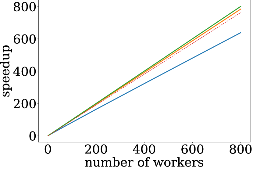
(c)

(d)

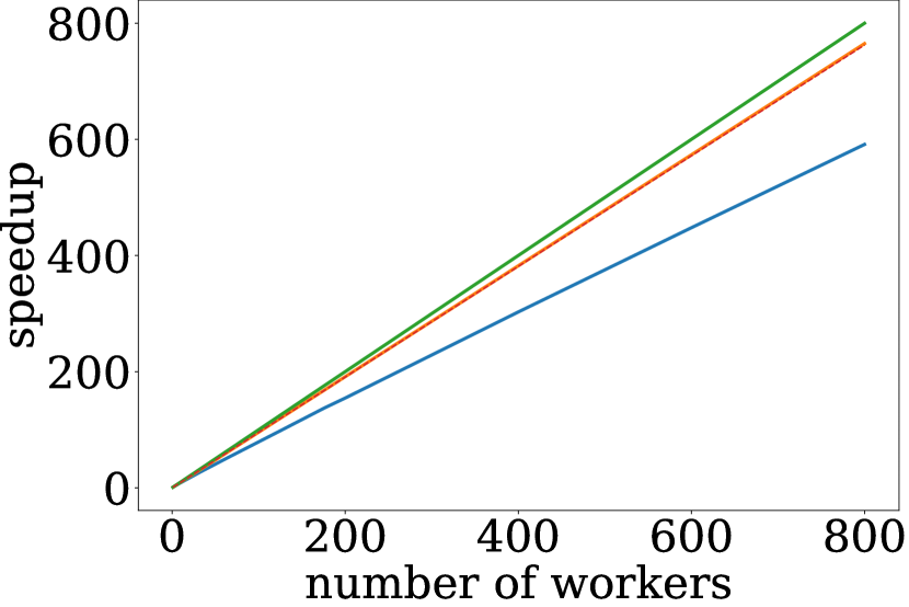
(e)

(f)

Figure 13: The noise distribution type impacts the effectiveness of DropCompute. Simulated scale graphs for a run with 12 accumulations. The duration of each accumulation is set to $0.45+\epsilon$ seconds Different sub-graphs exhibit different distributions for $\epsilon$. The bottom-right graph was drawn using the approximation from equation 6.

figure	Mean($\epsilon$)	Var($\epsilon$)	$\epsilon$ distribution		$\mathbb{E}[T]/\mathbb{E}[T_{i}]$
a	0.225	0.05	lognormal	$LN(\mu=-1.84,\sigma=0.83)$	1.496
b	0.225	0.05	normal	$\mathcal{N}(\mu=0.23,\sigma=0.22)$	1.302
c	0.225	0.05	bernoulli	$0.45Br(p=0.5)$	1.283
d	0.225	0.05	exponential	$exp(\lambda=4.47)$	1.386
e	0.225	0.05	gamma	$\gamma(\alpha=1,\beta=4.5)$	1.39

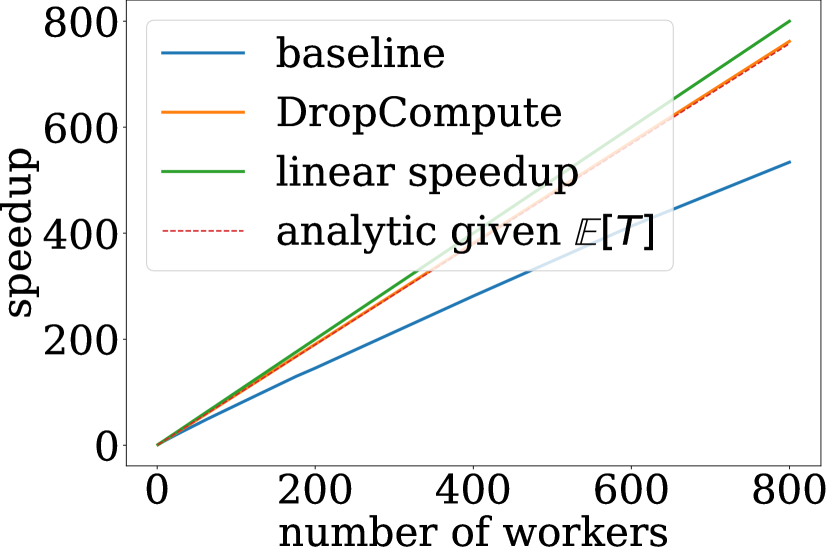
(a)

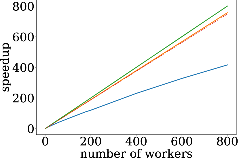
(b)

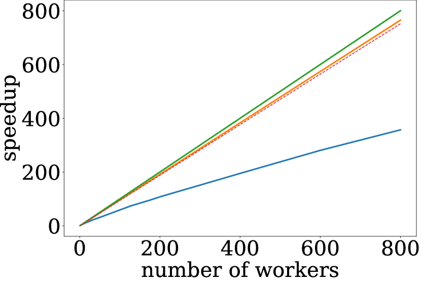
(c)

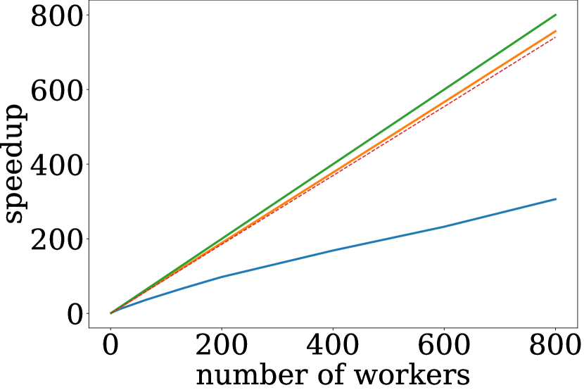
(d)

(e)

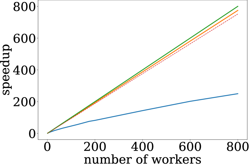
(f)

Figure 14: DropCompute increases robustness to the noise variance. Simulated scale graphs for a run with 12 accumulations. The duration of each accumulation is set to $0.45+\epsilon$ seconds. $\epsilon$ is a stochastic lognormal random variable with a mean of $0.225$ and changing variance, according to the table below

figure	Mean($\epsilon$)	Var($\epsilon$)	$\epsilon$ distribution		$\mathbb{E}[T]/\mathbb{E}[T_{i}]$
a	0.225	0.05	lognormal	$LN(\mu=-1.84,\sigma=0.83)$	1.496
b	0.225	0.1	lognormal	$LN(\mu=-2.04,\sigma=1.04)$	1.933
c	0.225	0.15	lognormal	$LN(\mu=-2.18,\sigma=1.17)$	2.394
d	0.225	0.2	lognormal	$LN(\mu=-2.29,\sigma=1.26)$	2.773
e	0.225	0.25	lognormal	$LN(\mu=-2.38,\sigma=1.33)$	3.043
f	0.225	0.3	lognormal	$LN(\mu=-2.46,\sigma=1.39)$	3.4

Appendix D Convergence with stochastic batch size

In this section, we provide proof of theorem 4.1 (D.2), as well as convergence proof for the loss itself in the convex case (D.1). We also discuss the generalization properties with a stochastic batch in section D.4.

D.1 Proof for convex case

Theorem D.1.

Under assumption 4.1 and the specific case where $f$ is a convex function, for SGD with DropCompute (Algorithm 1), given $N$ workers and a local batch size $b_{local}$, we have that

$$\mathbb{E}[\mathcal{L}(\mathcal{D},\bar{\theta})-\mathcal{L}(\mathcal{D},\theta^{*})]\leq\frac{8Lb_{\mathrm{max}}\|\theta_{1}-\theta^{*}\|^{2}}{K}+\frac{6\sigma\|\theta_{1}-\theta^{*}\|}{\sqrt{K}}~{}.$$ (13)

where $K$ is the total number of samples used throughout the algorithm , and the expectation is with respect to the randomization introduced due to sampling from $\mathcal{D}$ throughout the optimization process.

Proof of theorem D.1

Notation: During the proof we denote by $b_{i}$ the total batch size (summed over all workers) that we employ at iteration $i$. $K=\sum_{i=1}^{S}b_{i}$ is the total number of samples along all $S$ iterations. At iteration $i$ we maintain a weight vector $\theta_{i}\in{\mathbb{R}}^{d}$ and query a gradient estimate $g_{i}$ based on a batch size of $b_{i}$ samples. Thus, we set

$$g_{i}=\frac{1}{b_{i}}\sum_{s=1}^{b_{i}}g_{i}^{s}$$

where $g_{i}^{s}=\nabla\ell(z_{i}^{s},\theta_{i})$, and $z_{i}^{s}$ is randomly sampled from $\mathcal{D}$. We also maintain importance weights, $\alpha_{i}=b_{i}$.

Note that there exists $b_{\max}$ such that $\alpha_{i}\leq b_{\max}~{};\forall i$

Now, the update rule:

$$\theta_{i+1}=\theta_{i}-\eta\alpha_{i}g_{i}$$ (14)

Eventually, we output

$$\bar{\theta}=\frac{1}{\alpha_{1:S}}\sum_{i=1}^{S}\alpha_{i}\theta_{i}$$

where $\alpha_{1:S}:=\sum_{i=1}^{S}\alpha_{i}.$

We assume that the batch sizes $b_{i}$ are stopping times w.r.t. the natural filtration induced by the samples we draw during the optimization process. Informally, this means that the value of $b_{i}$ depends only on the history of the samples that we have seen prior to setting $b_{i}$.

We can therefore prove the following lemma,

Lemma D.1.

Upon choosing $\alpha_{i}=b_{i}$ the following holds,

$$\mathbb{E}[\alpha_{i}(g_{i}-\nabla\mathcal{L}(\mathcal{D},\theta_{i})|\theta_{i}]=\mathbb{E}[\sum_{s=1}^{b_{i}}(g_{i}^{s}-\nabla\mathcal{L}(\mathcal{D},\theta_{i}))|\theta_{i}]=0~{}.$$

Now, using standard analysis for Online Gradient Descent (Hazan et al., 2016) with the update rule of (14) gives,

$$\sum_{i=1}^{S}\alpha_{i}g_{i}\cdot(\theta_{i}-\theta^{*})\leq\frac{\|\theta_{1}-\theta^{*}\|^{2}}{\eta}+\eta\sum_{i=1}^{S}\alpha_{i}^{2}\|g_{i}\|^{2}$$

Taking expectation and using Lemma D.1 gives,

$$\mathbb{E}\sum_{i=1}^{S}\alpha_{i}\nabla\mathcal{L}(\mathcal{D},\theta_{i})\cdot(\theta_{i}-\theta^{*})\leq\frac{\|\theta_{1}-\theta^{*}\|^{2}}{\eta}+\eta\mathbb{E}\sum_{i=1}^{S}\alpha_{i}^{2}\|g_{i}\|^{2}$$

From convexity we know that $0\leq\mathcal{L}(\mathcal{D},\theta_{i})-\mathcal{L}(\mathcal{D},\theta^{*})\leq\nabla\mathcal{L}(\mathcal{D},\theta_{i})\cdot(\theta_{i}-\theta^{*})$, therefore the above implies,

$$\mathbb{E}\sum_{i=1}^{S}\alpha_{i}(\mathcal{L}(\mathcal{D},\theta_{i})-\mathcal{L}(\mathcal{D},\theta^{*}))\leq\frac{\|\theta_{1}-\theta^{*}\|^{2}}{\eta}+\eta\mathbb{E}\sum_{i=1}^{S}\alpha_{i}^{2}\|g_{i}\|^{2}$$ (15)

Now, we write $g_{i}=\nabla\mathcal{L}(\mathcal{D},\theta_{i})+\xi_{i}$ where $\xi_{i}=g_{i}-\nabla\mathcal{L}(\mathcal{D},\theta_{i})$ and note that

$$\alpha_{i}\xi_{i}=\sum_{s=1}^{b_{i}}(g_{i}^{s}-\nabla\mathcal{L}(\mathcal{D},\theta_{i}))=\sum_{s=1}^{b_{i}}\xi_{i}^{i}$$

where we denote $\xi_{i}^{s}:=g_{i}^{s}-\nabla\mathcal{L}(\mathcal{D},\theta_{i})$. Next, we shall use the following lemma,

Lemma D.2.

The following holds,

$$\mathbb{E}\alpha_{i}^{2}\|g_{i}\|^{2} \leq 2b_{\max}\mathbb{E}\alpha_{i}\|\nabla\mathcal{L}(\mathcal{D},\theta_{i})\|^{2}+2\sigma^{2}\mathbb{E}b_{i}~{}.$$ (16)

Moreover, due to the $L$-smoothness of $f(\cdot)$, and global optimality of $\theta^{*}$, the following holds,

$$\mathbb{E}\alpha_{i}^{2}\|g_{i}\|^{2} \leq 4b_{\max}L\mathbb{E}\alpha_{i}(\mathcal{L}(\mathcal{D},\theta_{i})-\mathcal{L}(\mathcal{D},\theta^{*}))+2\sigma^{2}\mathbb{E}b_{i}~{}.$$ (17)

Final Bound:

Plugging the above lemma back into Eq. (15) gives,

$$\mathbb{E}\sum_{i=1}^{S}\alpha_{i}(\mathcal{L}(\mathcal{D},\theta_{i})-\mathcal{L}(\mathcal{D},\theta^{*})) \leq\frac{\|\theta_{1}-\theta^{*}\|^{2}}{\eta}+4\eta b_{\max}\mathbb{E}\sum_{i=1}^{S}\alpha_{i}L(\mathcal{L}(\mathcal{D},\theta_{i})-\mathcal{L}(\mathcal{D},\theta^{*}))+8\eta\sigma^{2}\mathbb{E}\sum_{i=1}^{S}b_{i}$$

$$\leq\frac{\|\theta_{1}-\theta^{*}\|^{2}}{\eta}+4\eta b_{\max}L\mathbb{E}\sum_{i=1}^{S}\alpha_{i}(\mathcal{L}(\mathcal{D},\theta_{i})-\mathcal{L}(\mathcal{D},\theta^{*}))+8\eta\sigma^{2}K~{},$$ (18)

where we used $K=\sum_{i=1}^{S}b_{i}$.

Now if we pick $\eta$ such that $4\eta b_{\max}L\leq 1/2$ then we can move the second term in the RHS to the LHS and obtain,

$$\frac{1}{2}\mathbb{E}\sum_{i=1}^{S}\alpha_{i}(\mathcal{L}(\mathcal{D},\theta_{i})-\mathcal{L}(\mathcal{D},\theta^{*})) \leq\frac{\|\theta_{1}-\theta^{*}\|^{2}}{\eta}+8\eta\sigma^{2}K~{},$$ (19)

Thus, choosing $\eta=\min\left\{\frac{\|\theta_{1}-\theta^{*}\|}{\sigma\sqrt{8K}},\frac{1}{8Lb_{\max}}\right\}$ gives the following bound,

$$\mathbb{E}\sum_{i=1}^{S}\alpha_{i}(\mathcal{L}(\mathcal{D},\theta_{i})-\mathcal{L}(\mathcal{D},\theta^{*})) \leq 8Lb_{\max}\|\theta_{1}-\theta^{*}\|^{2}+6\sigma\|\theta_{1}-\theta^{*}\|\sqrt{K}$$ (20)

Now, recalling that $K:=\sum_{i=1}^{S}b_{i}=\sum_{i=1}^{S}\alpha_{i}$ and using Jensen’s inequality together with $\bar{\theta}=\frac{1}{\alpha_{1:S}}\sum_{i=1}^{S}\alpha_{i}\theta_{i}$ yields,

$$\mathbb{E}[\mathcal{L}(\mathcal{D},\bar{\theta})-\mathcal{L}(\mathcal{D},\theta^{*})] \leq\mathbb{E}\sum_{i=1}^{S}\frac{\alpha_{i}}{\alpha_{1:S}}(\mathcal{L}(\mathcal{D},\theta_{i})-\mathcal{L}(\mathcal{D},\theta^{*}))\leq\frac{8Lb_{\max}\|\theta_{1}-\theta^{*}\|^{2}+6\sigma\|\theta_{1}-\theta^{*}\|\sqrt{K}}{\alpha_{1:S}}$$

$$\leq\frac{8Lb_{\max}\|\theta_{1}-\theta^{*}\|^{2}}{K}+\frac{6\sigma\|\theta_{1}-\theta^{*}\|}{\sqrt{K}}$$ (21)

where we used $\alpha_{1:S}=K$.      ∎

D.2 Proof for non-convex case

Proof of theorem 4.1

We use the same notation for $b_{i}$ and $g_{i}$ as before. And again used weights,

$$\alpha_{i}=b_{i}$$

We also assume that $b_{i}\leq b_{\max}~{},\forall i$.

The update rule is the following,

$$\theta_{i+1}=\theta_{i}-\eta\alpha_{i}g_{i}$$

And the output is $\bar{\theta}$, where we define,

$$\bar{\theta}=\theta_{i}~{};\quad\text{w.p.}~{}~{}\frac{\alpha_{i}}{\alpha_{1:S}}$$

Thus,

$$\mathbb{E}\|\nabla\mathcal{L}(\mathcal{D},\bar{\theta})\|^{2}=\frac{1}{\alpha_{1:S}}\sum_{i=1}^{S}\alpha_{i}\mathbb{E}\|\nabla\mathcal{L}(\mathcal{D},\theta_{i})\|^{2}$$

Using smoothness,

$$\mathcal{L}(\mathcal{D},\theta_{i+1}) \leq\mathcal{L}(\mathcal{D},\theta_{i})-\nabla\mathcal{L}(\mathcal{D},\theta_{i})\cdot(\theta_{i+1}-\theta_{i})+\frac{L}{2}\|\theta_{i+1}-\theta_{i}\|^{2}$$

$$\leq\mathcal{L}(\mathcal{D},\theta_{i})-\eta\alpha_{i}\nabla\mathcal{L}(\mathcal{D},\theta_{i})\cdot g_{i}+\frac{L\eta^{2}}{2}\|\alpha_{i}g_{i}\|^{2}$$

$$\leq\mathcal{L}(\mathcal{D},\theta_{i})-\eta\alpha_{i}\|\nabla\mathcal{L}(\mathcal{D},\theta_{i})\|^{2}-\eta\alpha_{i}\nabla\mathcal{L}(\mathcal{D},\theta_{i})\cdot(g_{i}-\nabla\mathcal{L}(\mathcal{D},\theta_{i}))+\frac{L\eta^{2}}{2}\|\alpha_{i}g_{i}\|^{2}$$

Re-arranging the above yields,

$$\eta\alpha_{i}\|\nabla\mathcal{L}(\mathcal{D},\theta_{i})\|^{2} \leq\mathcal{L}(\mathcal{D},\theta_{i})-\mathcal{L}(\mathcal{D},\theta_{i+1})-\eta\alpha_{i}\nabla\mathcal{L}(\mathcal{D},\theta_{i})\cdot(g_{i}-\nabla\mathcal{L}(\mathcal{D},\theta_{i}))+\frac{L\eta^{2}}{2}\|\alpha_{i}g_{i}\|^{2}$$

Summing the above, and dividing by $\eta$, we obtain,

$$\sum_{i=1}^{S}\alpha_{i}\|\nabla\mathcal{L}(\mathcal{D},\theta_{i})\|^{2} \leq\frac{1}{\eta}(\mathcal{L}(\mathcal{D},\theta_{1})-\mathcal{L}(\mathcal{D},\theta_{S+1}))-\sum_{i=1}^{S}\alpha_{i}\nabla\mathcal{L}(\mathcal{D},\theta_{i})\cdot(g_{i}-\nabla\mathcal{L}(\mathcal{D},\theta_{i}))+\frac{L\eta}{2}\sum_{i=1}^{S}\|\alpha_{i}g_{i}\|^{2}$$

$$\leq\frac{1}{\eta}(\mathcal{L}(\mathcal{D},\theta_{1})-\mathcal{L}(\mathcal{D},\theta^{*}))-\sum_{i=1}^{S}\alpha_{i}\nabla\mathcal{L}(\mathcal{D},\theta_{i})\cdot(g_{i}-\nabla\mathcal{L}(\mathcal{D},\theta_{i}))+\frac{L\eta}{2}\sum_{i=1}^{S}\|\alpha_{i}g_{i}\|^{2}$$ (22)

where we uses $\mathcal{L}(\mathcal{D},\theta^{*})\leq\mathcal{L}(\mathcal{D},\theta_{S+1})$ since $\theta^{*}$ is the global minimum of $\mathcal{L}(\mathcal{D},\cdot)$.

Now recall that from Lemma D.1 we have,

$$\mathbb{E}[\alpha_{i}(g_{i}-\nabla\mathcal{L}(\mathcal{D},\theta_{i}))|\theta_{i}]=0~{}.$$ (23)

And from Lemma D.2 we have,

$$\mathbb{E}\alpha_{i}^{2}\|g_{i}\|^{2} \leq 2b_{\max}\mathbb{E}\alpha_{i}\|\nabla\mathcal{L}(\mathcal{D},\theta_{i})\|^{2}+2\sigma^{2}\mathbb{E}b_{i}~{}.$$ (24)

Thus, taking expectation in Eq. (D.2), and plugging Eq. (23) and (24), yields,

$$\mathbb{E}\sum_{i=1}^{S}\alpha_{i}\|\nabla\mathcal{L}(\mathcal{D},\theta_{i})\|^{2} \leq\frac{1}{\eta}(\mathcal{L}(\mathcal{D},\theta_{1})-\mathcal{L}(\mathcal{D},\theta^{*}))-\sum_{i=1}^{S}\mathbb{E}\alpha_{i}\nabla\mathcal{L}(\mathcal{D},\theta_{i})\cdot(g_{i}-\nabla\mathcal{L}(\mathcal{D},\theta_{i}))+\frac{L\eta}{2}\sum_{i=1}^{S}\mathbb{E}\|\alpha_{i}g_{i}\|^{2}$$

$$\leq\frac{1}{\eta}(\mathcal{L}(\mathcal{D},\theta_{1})-\mathcal{L}(\mathcal{D},\theta^{*}))+L\eta b_{\max}\sum_{i=1}^{S}\mathbb{E}\alpha_{i}\|\nabla\mathcal{L}(\mathcal{D},\theta_{i})\|^{2}+L\eta\sigma^{2}\mathbb{E}\sum_{i=1}^{S}b_{i}$$

$$\leq\frac{1}{\eta}(\mathcal{L}(\mathcal{D},\theta_{1})-\mathcal{L}(\mathcal{D},\theta^{*}))+L\eta b_{\max}\sum_{i=1}^{S}\mathbb{E}\alpha_{i}\|\nabla\mathcal{L}(\mathcal{D},\theta_{i})\|^{2}+L\eta\sigma^{2}\cdot K$$ (25)

where the last line uses $K:=\sum_{i=1}^{S}b_{i}$.

Now if we pick $\eta$ such that $\eta b_{\max}L\leq 1/2$ then we can move the second term in the RHS to the LHS and obtain,

$$\frac{1}{2}\mathbb{E}\sum_{i=1}^{S}\alpha_{i}\|\nabla\mathcal{L}(\mathcal{D},\theta_{i})\|^{2} \leq\frac{1}{\eta}(\mathcal{L}(\mathcal{D},\theta_{1})-\mathcal{L}(\mathcal{D},\theta^{*}))+L\eta\sigma^{2}\cdot K$$ (26)

Thus, choosing $\eta=\min\left\{\frac{\sqrt{\mathcal{L}(\mathcal{D},\theta_{1})-\mathcal{L}(\mathcal{D},\theta^{*})}}{\sigma\sqrt{LK}},\frac{1}{2Lb_{\max}}\right\}$ gives the following bound,

$$\mathbb{E}\sum_{i=1}^{S}\alpha_{i}\|\nabla\mathcal{L}(\mathcal{D},\theta_{i})\|^{2} \leq 2Lb_{\max}(\mathcal{L}(\mathcal{D},\theta_{1})-\mathcal{L}(\mathcal{D},\theta^{*}))+2\sigma\sqrt{L(\mathcal{L}(\mathcal{D},\theta_{1})-\mathcal{L}(\mathcal{D},\theta^{*}))}\cdot\sqrt{K}$$ (27)

Dividing by $K:=\alpha_{1:S}$ and using the definition of $\bar{\theta}$ yields,

$$\mathbb{E}\|\nabla\mathcal{L}(\mathcal{D},\bar{\theta})\|^{2}=\mathbb{E}\frac{1}{\alpha_{1:S}}\sum_{i=1}^{S}\alpha_{i}\|\nabla\mathcal{L}(\mathcal{D},\theta_{i})\|^{2} \leq\frac{2Lb_{\max}(\mathcal{L}(\mathcal{D},\theta_{1})-\mathcal{L}(\mathcal{D},\theta^{*}))}{K}+\frac{2\sigma\sqrt{L(\mathcal{L}(\mathcal{D},\theta_{1})-\mathcal{L}(\mathcal{D},\theta^{*}))}}{\sqrt{K}}$$ (28)

D.3 Remaining Proofs

D.3.1 Proof of Lemma D.2

Proof of Lemma D.2.

We can write,

$$\alpha_{i}^{2}\|g_{i}\|^{2} =\|b_{i}\nabla\mathcal{L}(\mathcal{D},\theta_{i})+\sum_{s=1}^{b_{i}}\xi_{i}^{s}\|^{2}$$

$$\leq 2\|b_{i}\nabla\mathcal{L}(\mathcal{D},\theta_{i})\|^{2}+2\|\sum_{s=1}^{b_{i}}\xi_{i}^{s}\|^{2}$$

$$=2b_{i}^{2}\|\nabla\mathcal{L}(\mathcal{D},\theta_{i})\|^{2}+2\|\sum_{s=1}^{b_{i}}\xi_{i}^{s}\|^{2}$$

$$\leq 2b_{\max}\alpha_{i}\|\nabla\mathcal{L}(\mathcal{D},\theta_{i})\|^{2}+2\|\sum_{s=1}^{b_{i}}\xi_{i}^{s}\|^{2}$$

where the second line uses $\|a+b\|^{2}\leq 2\|a\|^{2}+2\|b\|^{2}$; the fourth line uses $b_{i}\leq b_{\max}$ as well as $\alpha_{i}=b_{i}$ implying that $b_{i}^{2}\leq b_{\max}\alpha_{i}$.

Bounding $E\|\sum_{s=1}^{b_{i}}\xi_{i}^{s}\|^{2}$:

Given $i$ and $\theta_{i}$, Let us define the following sequence, $Q_{0}=0$, $Q_{1}=\|\xi_{i}^{1}\|^{2}-\sigma$, and for any $k>1$

$$Q_{k}=\sum_{s=1}^{k}\|\xi_{i}^{k}\|^{2}-\sigma^{2}\cdot k+2\sum_{s=1}^{j}\sum_{n=s+1}^{j}\xi_{i}^{s}\cdot\xi_{i}^{n}$$

It can be directly shown that $\{Q_{k}\}_{k}$ is a Supermartingale sequence, and that

$$\|\sum_{s=1}^{b_{i}}\xi_{i}^{s}\|^{2}=Q_{b_{i}}+\sigma^{2}\cdot b_{i}$$

Thus, since $b_{i}$ is a bounded stopping time, we can use Doob’s optional stopping theorem which implies that,

$$\mathbb{E}\|\sum_{s=1}^{b_{i}}\xi_{i}^{s}\|^{2}=\mathbb{E}Q_{b_{i}}+\sigma^{2}\mathbb{E}\cdot b_{i}\leq EQ_{0}+\sigma^{2}\mathbb{E}\cdot b_{i}=0+\sigma^{2}\mathbb{E}b_{i}$$

Plugging the above back into Eq. (D.3.1) yields,

$$\mathbb{E}\alpha_{i}^{2}\|g_{i}\|^{2} \leq 2b_{\max}\mathbb{E}\alpha_{i}\|\nabla\mathcal{L}(\mathcal{D},\theta_{i})\|^{2}+2\sigma^{2}\mathbb{E}b_{i}~{}.$$ (30)

Now, since $\mathcal{L}(\mathcal{D},\cdot)$ is $L$-smooth and $\theta^{*}$ is its global minima, then the following holds: $\|\nabla\mathcal{L}(\mathcal{D},\theta_{i})\|^{2}\leq 2L(\mathcal{L}(\mathcal{D},\theta_{i})-\mathcal{L}(\mathcal{D},\theta^{*}))$; See e.g. Levy (2017) for the proof. Plugging this into the above equation we obtain,

$$\mathbb{E}\alpha_{i}^{2}\|g_{i}\|^{2} \leq 4b_{\max}\mathbb{E}\alpha_{i}L(\mathcal{L}(\mathcal{D},\theta_{i})-\mathcal{L}(\mathcal{D},\theta^{*}))+2\sigma^{2}\mathbb{E}b_{i}~{}.$$ (31)

∎

D.3.2 Proof of Lemma D.1

Proof of Lemma D.1.

We can define the following Martingale sequence for each step $s$: $M_{0}=0$, and $M_{j}=\sum_{s=1}^{j}(g_{i}^{s}-\nabla\mathcal{L}(\mathcal{D},\theta_{i}))$ for any $j=1,2,\ldots$.

Thus, since the mixing time $b_{i}$ is bounded by $b_{\max}$, then according to Doob’s optional stopping theorem (Levin & Peres, 2017) we have that,

$$\mathbb{E}[M_{b_{i}}|\theta_{i}]=\mathbb{E}[\sum_{s=1}^{b_{i}}(g_{i}^{s}-\nabla\mathcal{L}(\mathcal{D},\theta_{i}))|\theta_{i}]=\mathbb{E}[M_{0}|\theta_{i}]=0~{}.$$ (32)

Now, notice that for any $i$, we have $\alpha_{i}(g_{i}-\nabla\mathcal{L}(\mathcal{D},\theta_{i}))=M_{b_{i}}$, and therefore,

$$\mathbb{E}[\alpha_{i}(g_{i}-\nabla\mathcal{L}(\mathcal{D},\theta_{i}))|\theta_{i}]=\mathbb{E}[M_{b_{i}}|\theta_{i}]=0~{}.$$ (33)

∎

D.4 Generalization discussion

An interesting observation arising from our results is the small impact of gradient dropping as measured in final test accuracy. One explanation for this can be based on viewing DropCompute as noise induced over gradients. Optimization using variants of SGD is inherently noisy due to the use of data samples used to evaluate the intermediate error. The stochastic nature of computed weight gradients was previously found to provide generalization benefits for the final trained model, although this is still part of ongoing debate (Geiping et al., 2022). Nevertheless, several works found generalization benefits with the injection of noise into the weights’ gradients (Neelakantan et al., 2015) or their use in computed update rule (Lin et al., 2022).

References

- Assran et al. (2019) Mahmoud Assran, Nicolas Loizou, Nicolas Ballas, and Mike Rabbat. Stochastic gradient push for distributed deep learning. In International Conference on Machine Learning, pp. 344–353. PMLR, 2019.
- Bailey et al. (2014) David H Bailey, Jonathan M Borwein, Marcos López de Prado, and Qiji Jim Zhu. Pseudomathematics and financial charlatanism: The effects of backtest over fitting on out-of-sample performance. Notices of the AMS, 61(5):458–471, 2014.
- Ben-Nun & Hoefler (2019) Tal Ben-Nun and Torsten Hoefler. Demystifying parallel and distributed deep learning: An in-depth concurrency analysis. ACM Comput. Surv., 52(4), aug 2019. ISSN 0360-0300. doi: 10.1145/3320060. URL https://doi.org/10.1145/3320060.
- Bitar et al. (2020) Rawad Bitar, Mary Wootters, and Salim El Rouayheb. Stochastic gradient coding for straggler mitigation in distributed learning. IEEE Journal on Selected Areas in Information Theory, 1(1):277–291, 2020.
- Chen et al. (2020) Chia-Yu Chen, Jiamin Ni, Songtao Lu, Xiaodong Cui, Pin-Yu Chen, Xiao Sun, Naigang Wang, Swagath Venkataramani, Vijayalakshmi Viji Srinivasan, Wei Zhang, et al. Scalecom: Scalable sparsified gradient compression for communication-efficient distributed training. Advances in Neural Information Processing Systems, 33:13551–13563, 2020.
- Chen et al. (2016) Jianmin Chen, Xinghao Pan, Rajat Monga, Samy Bengio, and Rafal Jozefowicz. Revisiting distributed synchronous sgd. arXiv preprint arXiv:1604.00981, 2016.
- Chowdhery et al. (2022) Aakanksha Chowdhery, Sharan Narang, Jacob Devlin, Maarten Bosma, Gaurav Mishra, Adam Roberts, Paul Barham, Hyung Won Chung, Charles Sutton, Sebastian Gehrmann, et al. Palm: Scaling language modeling with pathways. arXiv preprint arXiv:2204.02311, 2022.
- Dehghani et al. (2023) Mostafa Dehghani, Basil Mustafa, Josip Djolonga, Jonathan Heek, Matthias Minderer, Mathilde Caron, Andreas Steiner, Joan Puigcerver, Robert Geirhos, Ibrahim Alabdulmohsin, et al. Patch n’pack: Navit, a vision transformer for any aspect ratio and resolution. arXiv preprint arXiv:2307.06304, 2023.
- Dekel et al. (2012) Ofer Dekel, Ran Gilad-Bachrach, Ohad Shamir, and Lin Xiao. Optimal distributed online prediction using mini-batches. Journal of Machine Learning Research, 13(1), 2012.
- Deng et al. (2009) J. Deng, W. Dong, R. Socher, L.-J. Li, K. Li, and L. Fei-Fei. ImageNet: A Large-Scale Hierarchical Image Database. In CVPR09, 2009.
- Devlin et al. (2018) Jacob Devlin, Ming-Wei Chang, Kenton Lee, and Kristina Toutanova. Bert: Pre-training of deep bidirectional transformers for language understanding. arXiv preprint arXiv:1810.04805, 2018.
- Geiping et al. (2022) Jonas Geiping, Micah Goldblum, Phil Pope, Michael Moeller, and Tom Goldstein. Stochastic training is not necessary for generalization. In International Conference on Learning Representations, 2022. URL https://openreview.net/forum?id=ZBESeIUB5k.
- Giladi et al. (2019) Niv Giladi, Mor Shpigel Nacson, Elad Hoffer, and Daniel Soudry. At stability’s edge: How to adjust hyperparameters to preserve minima selection in asynchronous training of neural networks? arXiv preprint arXiv:1909.12340, 2019.
- Goyal et al. (2017) Priya Goyal, Piotr Dollár, Ross Girshick, Pieter Noordhuis, Lukasz Wesolowski, Aapo Kyrola, Andrew Tulloch, Yangqing Jia, and Kaiming He. Accurate, large minibatch sgd: Training imagenet in 1 hour. arXiv preprint arXiv:1706.02677, 2017.
- Habana (2020) Habana. Habana gaudi training whitepaper, June 2020. URL https://habana.ai/wp-content/uploads/pdf/2020/Habana%20GAUDI%20Training%20Whitepaper%20v1.2.pdf.
- Habana (2023) Habana. Pre-training the bert 1.5b model with deepspeed, January 2023. URL https://developer.habana.ai/blog/pre-training-the-bert-1-5b-model-with-deepspeed/.
- Hazan et al. (2016) Elad Hazan et al. Introduction to online convex optimization. Foundations and Trends® in Optimization, 2(3-4):157–325, 2016.
- He et al. (2015) Kaiming He, Xiangyu Zhang, Shaoqing Ren, and Jian Sun. Deep residual learning for image recognition, 2015.
- Hoefler et al. (2010) Torsten Hoefler, Timo Schneider, and Andrew Lumsdaine. Characterizing the influence of system noise on large-scale applications by simulation. In SC’10: Proceedings of the 2010 ACM/IEEE International Conference for High Performance Computing, Networking, Storage and Analysis, pp. 1–11. IEEE, 2010.
- Hoffer et al. (2017) Elad Hoffer, Itay Hubara, and Daniel Soudry. Train longer, generalize better: closing the generalization gap in large batch training of neural networks. Advances in neural information processing systems, 30, 2017.
- Hooker (2020) Sara Hooker. The hardware lottery. CoRR, abs/2009.06489, 2020. URL https://arxiv.org/abs/2009.06489.
- Jiang et al. (2017) Zhanhong Jiang, Aditya Balu, Chinmay Hegde, and Soumik Sarkar. Collaborative deep learning in fixed topology networks. Advances in Neural Information Processing Systems, 30, 2017.
- Kaplan et al. (2020) Jared Kaplan, Sam McCandlish, Tom Henighan, Tom B. Brown, Benjamin Chess, Rewon Child, Scott Gray, Alec Radford, Jeffrey Wu, and Dario Amodei. Scaling laws for neural language models, 2020. URL https://arxiv.org/abs/2001.08361.
- Kosec et al. (2021) Matej Kosec, Sheng Fu, and Mario Michael Krell. Packing: Towards 2x NLP BERT acceleration. CoRR, abs/2107.02027, 2021. URL https://arxiv.org/abs/2107.02027.
- Levin & Peres (2017) David A Levin and Yuval Peres. Markov chains and mixing times, volume 107. American Mathematical Soc., 2017.
- Levy (2017) Kfir Levy. Online to offline conversions, universality and adaptive minibatch sizes. Advances in Neural Information Processing Systems, 30, 2017.
- Li et al. (2020a) Shigang Li, Tal Ben-Nun, Giorgi Nadiradze, Salvatore Di Girolamo, Nikoli Dryden, Dan Alistarh, and Torsten Hoefler. Breaking (global) barriers in parallel stochastic optimization with wait-avoiding group averaging. IEEE Transactions on Parallel and Distributed Systems, 32(7):1725–1739, 2020a.
- Li et al. (2020b) Tian Li, Anit Kumar Sahu, Manzil Zaheer, Maziar Sanjabi, Ameet Talwalkar, and Virginia Smith. Federated optimization in heterogeneous networks. Proceedings of Machine learning and systems, 2:429–450, 2020b.
- Lian et al. (2017) Xiangru Lian, Ce Zhang, Huan Zhang, Cho-Jui Hsieh, Wei Zhang, and Ji Liu. Can decentralized algorithms outperform centralized algorithms? a case study for decentralized parallel stochastic gradient descent. Advances in Neural Information Processing Systems, 30, 2017.
- Lin et al. (2022) Huangxing Lin, Weihong Zeng, Yihong Zhuang, Xinghao Ding, Yue Huang, and John Paisley. Learning rate dropout. IEEE Transactions on Neural Networks and Learning Systems, pp. 1–11, 2022. doi: 10.1109/TNNLS.2022.3155181.
- Lin et al. (2020) Tao Lin, Sebastian U. Stich, Kumar Kshitij Patel, and Martin Jaggi. Don’t use large mini-batches, use local sgd. In International Conference on Learning Representations, 2020.
- Liu et al. (2019) Yinhan Liu, Myle Ott, Naman Goyal, Jingfei Du, Mandar Joshi, Danqi Chen, Omer Levy, Mike Lewis, Luke Zettlemoyer, and Veselin Stoyanov. Roberta: A robustly optimized bert pretraining approach, 2019. URL https://arxiv.org/abs/1907.11692.
- Mattson et al. (2019) Peter Mattson, Christine Cheng, Cody Coleman, Greg Diamos, Paulius Micikevicius, David A. Patterson, Hanlin Tang, Gu-Yeon Wei, Peter Bailis, Victor Bittorf, David Brooks, Dehao Chen, Debojyoti Dutta, Udit Gupta, Kim M. Hazelwood, Andrew Hock, Xinyuan Huang, Bill Jia, Daniel Kang, David Kanter, Naveen Kumar, Jeffery Liao, Guokai Ma, Deepak Narayanan, Tayo Oguntebi, Gennady Pekhimenko, Lillian Pentecost, Vijay Janapa Reddi, Taylor Robie, Tom St. John, Carole-Jean Wu, Lingjie Xu, Cliff Young, and Matei Zaharia. Mlperf training benchmark. CoRR, abs/1910.01500, 2019. URL http://arxiv.org/abs/1910.01500.
- Mitliagkas et al. (2016) Ioannis Mitliagkas, Ce Zhang, Stefan Hadjis, and Christopher Ré. Asynchrony begets momentum, with an application to deep learning. In 2016 54th Annual Allerton Conference on Communication, Control, and Computing (Allerton), pp. 997–1004. IEEE, 2016.
- Narayanan et al. (2021) Deepak Narayanan, Mohammad Shoeybi, Jared Casper, Patrick LeGresley, Mostofa Patwary, Vijay Korthikanti, Dmitri Vainbrand, Prethvi Kashinkunti, Julie Bernauer, Bryan Catanzaro, Amar Phanishayee, and Matei Zaharia. Efficient large-scale language model training on gpu clusters using megatron-lm. In Proceedings of the International Conference for High Performance Computing, Networking, Storage and Analysis, SC ’21, New York, NY, USA, 2021. Association for Computing Machinery. ISBN 9781450384421. doi: 10.1145/3458817.3476209. URL https://doi.org/10.1145/3458817.3476209.
- Neelakantan et al. (2015) Arvind Neelakantan, Luke Vilnis, Quoc V. Le, Ilya Sutskever, Lukasz Kaiser, Karol Kurach, and James Martens. Adding gradient noise improves learning for very deep networks, 2015. URL https://arxiv.org/abs/1511.06807.
- Nvidia (2023) Nvidia. mlcommons training results v3.0 gpt3. https://github.com/mlcommons/training_results_v3.0/tree/main/NVIDIA/benchmarks/gpt3/implementations/pytorch, 2023.
- Ott et al. (2018) Myle Ott, Sergey Edunov, David Grangier, and Michael Auli. Scaling neural machine translation. In Proceedings of the Third Conference on Machine Translation: Research Papers, pp. 1–9, Brussels, Belgium, October 2018. Association for Computational Linguistics. doi: 10.18653/v1/W18-6301. URL https://aclanthology.org/W18-6301.
- Patarasuk & Yuan (2009) Pitch Patarasuk and Xin Yuan. Bandwidth optimal all-reduce algorithms for clusters of workstations. Journal of Parallel and Distributed Computing, 69(2):117–124, 2009.
- Petrini et al. (2003) Fabrizio Petrini, Darren J Kerbyson, and Scott Pakin. The case of the missing supercomputer performance: Achieving optimal performance on the 8,192 processors of asci q. In Proceedings of the 2003 ACM/IEEE conference on Supercomputing, pp. 55, 2003.
- Radford et al. (2019) Alec Radford, Jeff Wu, Rewon Child, David Luan, Dario Amodei, and Ilya Sutskever. Language models are unsupervised multitask learners. 2019.
- Raffel et al. (2020a) Colin Raffel, Noam Shazeer, Adam Roberts, Katherine Lee, Sharan Narang, Michael Matena, Yanqi Zhou, Wei Li, and Peter J. Liu. Exploring the limits of transfer learning with a unified text-to-text transformer. Journal of Machine Learning Research, 21(140):1–67, 2020a. URL http://jmlr.org/papers/v21/20-074.html.
- Raffel et al. (2020b) Colin Raffel, Noam Shazeer, Adam Roberts, Katherine Lee, Sharan Narang, Michael Matena, Yanqi Zhou, Wei Li, and Peter J Liu. Exploring the limits of transfer learning with a unified text-to-text transformer. The Journal of Machine Learning Research, 21(1):5485–5551, 2020b.
- Rajbhandari et al. (2020) Samyam Rajbhandari, Jeff Rasley, Olatunji Ruwase, and Yuxiong He. Zero: Memory optimizations toward training trillion parameter models. In SC20: International Conference for High Performance Computing, Networking, Storage and Analysis, pp. 1–16. IEEE, 2020.
- Rajpurkar et al. (2016) Pranav Rajpurkar, Jian Zhang, Konstantin Lopyrev, and Percy Liang. SQuAD: 100,000+ questions for machine comprehension of text. In Proceedings of the 2016 Conference on Empirical Methods in Natural Language Processing, pp. 2383–2392, Austin, Texas, November 2016. Association for Computational Linguistics.
- Rasley et al. (2020) Jeff Rasley, Samyam Rajbhandari, Olatunji Ruwase, and Yuxiong He. Deepspeed: System optimizations enable training deep learning models with over 100 billion parameters. In Proceedings of the 26th ACM SIGKDD International Conference on Knowledge Discovery & Data Mining, pp. 3505–3506, 2020.
- Sanders et al. (2019) Peter Sanders, Kurt Mehlhorn, Martin Dietzfelbinger, and Roman Dementiev. Sequential and Parallel Algorithms and Data Structures. Springer, 2019.
- Scao et al. (2022) Teven Le Scao, Angela Fan, Christopher Akiki, Ellie Pavlick, Suzana Ilić, Daniel Hesslow, Roman Castagné, Alexandra Sasha Luccioni, François Yvon, Matthias Gallé, et al. Bloom: A 176b-parameter open-access multilingual language model. arXiv preprint arXiv:2211.05100, 2022.
- Seide et al. (2014) Frank Seide, Hao Fu, Jasha Droppo, Gang Li, and Dong Yu. 1-bit stochastic gradient descent and application to data-parallel distributed training of speech dnns. In Interspeech 2014, September 2014.
- Smith et al. (2022) Shaden Smith, Mostofa Patwary, Brandon Norick, Patrick LeGresley, Samyam Rajbhandari, Jared Casper, Zhun Liu, Shrimai Prabhumoye, George Zerveas, Vijay Korthikanti, et al. Using deepspeed and megatron to train megatron-turing nlg 530b, a large-scale generative language model. arXiv preprint arXiv:2201.11990, 2022.
- Sobkowicz et al. (2013) Pawel Sobkowicz, Mike Thelwall, Kevan Buckley, Georgios Paltoglou, and Antoni Sobkowicz. Lognormal distributions of user post lengths in internet discussions-a consequence of the weber-fechner law? EPJ Data Science, 2(1):1–20, 2013.
- Stich (2019) Sebastian U. Stich. Local SGD converges fast and communicates little. In International Conference on Learning Representations, 2019.
- Tan & Le (2021) Mingxing Tan and Quoc Le. Efficientnetv2: Smaller models and faster training. In International conference on machine learning, pp. 10096–10106. PMLR, 2021.
- Tang et al. (2021) Hanlin Tang, Shaoduo Gan, Ammar Ahmad Awan, Samyam Rajbhandari, Conglong Li, Xiangru Lian, Ji Liu, Ce Zhang, and Yuxiong He. 1-bit adam: Communication efficient large-scale training with adam’s convergence speed. In Marina Meila and Tong Zhang (eds.), Proceedings of the 38th International Conference on Machine Learning, volume 139 of Proceedings of Machine Learning Research, pp. 10118–10129. PMLR, 18–24 Jul 2021.
- Touvron et al. (2023) Hugo Touvron, Louis Martin, Kevin Stone, Peter Albert, Amjad Almahairi, Yasmine Babaei, Nikolay Bashlykov, Soumya Batra, Prajjwal Bhargava, Shruti Bhosale, et al. Llama 2: Open foundation and fine-tuned chat models. arXiv preprint arXiv:2307.09288, 2023.
- Vogels et al. (2019) Thijs Vogels, Sai Praneeth Karimireddy, and Martin Jaggi. Powersgd: Practical low-rank gradient compression for distributed optimization. Advances in Neural Information Processing Systems, 32, 2019.
- (57) U von Luxburg, S Bengio, HM Wallach, R Fergus, SVN Vishwanathan, and R Garnett. https://github. com/baidu-research/baidu-allreduce.
- Wang & Joshi (2021) Jianyu Wang and Gauri Joshi. Cooperative sgd: A unified framework for the design and analysis of local-update sgd algorithms. Journal of Machine Learning Research, 22, 2021.
- Wang et al. (2020) Jianyu Wang, Vinayak Tantia, Nicolas Ballas, and Michael Rabbat. Slowmo: Improving communication-efficient distributed sgd with slow momentum. In International Conference on Learning Representations, 2020.
- Xu et al. (2021) Hang Xu, Kelly Kostopoulou, Aritra Dutta, Xin Li, Alexandros Ntoulas, and Panos Kalnis. Deepreduce: A sparse-tensor communication framework for federated deep learning. Advances in Neural Information Processing Systems, 34:21150–21163, 2021.
- Yang et al. (2020) Donglin Yang, Wei Rang, and Dazhao Cheng. Mitigating stragglers in the decentralized training on heterogeneous clusters. In Proceedings of the 21st International Middleware Conference, pp. 386–399, 2020.
- You et al. (2017) Yang You, Igor Gitman, and Boris Ginsburg. Large batch training of convolutional networks. arXiv preprint arXiv:1708.03888, 2017.
- You et al. (2019) Yang You, Jing Li, Sashank Reddi, Jonathan Hseu, Sanjiv Kumar, Srinadh Bhojanapalli, Xiaodan Song, James Demmel, Kurt Keutzer, and Cho-Jui Hsieh. Large batch optimization for deep learning: Training bert in 76 minutes. arXiv preprint arXiv:1904.00962, 2019.
- Zhang et al. (2015) Sixin Zhang, Anna E Choromanska, and Yann LeCun. Deep learning with elastic averaging sgd. Advances in neural information processing systems, 28, 2015.
- Zheng et al. (2020) Shuai Zheng, Haibin Lin, Sheng Zha, and Mu Li. Accelerated large batch optimization of bert pretraining in 54 minutes, 2020.