A nonparametric test for elliptical distribution based on kernel embedding of probabilities

Abstract

Elliptical distribution is a basic assumption underlying many multivariate statistical methods. For example, in sufficient dimension reduction and statistical graphical models, this assumption is routinely imposed to simplify the data dependence structure. Before applying such methods, we need to decide whether the data are elliptically distributed. Currently existing tests either focus exclusively on spherical distributions, or rely on bootstrap to determine the null distribution, or require specific forms of the alternative distribution. In this paper, we introduce a general nonparametric test for elliptical distribution based on kernel embedding of the probability measure that embodies the two properties that characterize an elliptical distribution: namely, after centering and rescaling, (1) the direction and length of the random vector are independent, and (2) the directional vector is uniformly distributed on the unit sphere. We derive the null asymptotic distribution of the test statistic via von-Mises expansion, develop the sample-level procedure to determine the rejection region, and establish the consistency and validity of the proposed test. We apply our test to a SENIC dataset with and without a transformation aimed to achieve ellipticity.

and

1 Introduction

Elliptical distribution is a widely-used assumption for many statistical and machine learning methods for multivariate data. For example, in sufficient dimension reduction, the elliptical distribution assumption for the predictor is needed for moment-based methods such as Sliced Inverse Regression (Li, 1991), Ordinary Least Squares (Li and Duan, 1989), and Iterative Hessian Transformation (Cook and Li, 2002). See also Li (2018). When this assumption is violated, one needs either to perform data transformation or to modify the inverse-regression methods as did in Li and Dong (2009). Another example is the statistical graphical model, where a class of methods, such as glasso (Yuan and Lin, 2006) and the transelliptical graphical model (Liu, Han and Zhang, 2012), require either a Gaussian or an elliptical distribution. See also Vogel and Fried (2011), which introduces a class elliptical graphical models as a robust alternative to the Gaussian graphical model.

There are some existing tests on spherical distributions. For example, Baringhaus (1991) proposes a test based on the $L^{2}$-distance between the empirical distribution of the data and the distribution function partially specified by the spherical assumption. Liang, Fang and Hickernell (2008) introduces a necessary test by applying the Rosenblatt transformation on each element. The hypothesis in this test is necessary in the sense that it is implied by spherical distribution but does not imply the spherical distribution. Henze, Hlávka and Meintanis (2014) introduces a test by checking whether the characteristic function is constant over surfaces of spheres centered at the origin. Kariya and Eaton (1977) introduces a robust test of a spherical distribution centered at the origin against an elliptical or a noncentered spherical distribution. Koltchinskii and Li (1998) uses the multivariate distribution and quantile functions to test spherical distributions with unknown centers. All tests above are for the spherical distributions where the covariance matrix is exactly the identity matrix, and most of them focus on the case when we know the center is zero. These methods do not yield direct extensions for testing elliptical distributions where both the mean vector and covariance matrix are unknown.

There also exist some tests on elliptical distributions. Huffer and Park (2007) gives a test for multivariate normal and elliptical distribution of the data based on a chi-square statistic after slicing the data. For the multivariate normal distribution, they derive the asymptotic null distribution of their test; for the elliptical distribution, they propose a bootstrap test without giving a proof of its consistency and validity. Albisetti, Balabdaoui and Holzmann (2020) introduces a test based on a Kolmogorov-Smirnov type statistic and uses bootstrap to construct the null distribution. Manzotti, Pérez and Quiroz (2002) proposes a test on whether the standardized directional vector is uniformly distributed on the unit sphere, which is, again, only a necessary condition for spherical distribution. Babic et al. (2019) develops optimal tests for elliptical distributions against some generalized skew-elliptical alternatives.

In this paper, we introduce a nonparametric test for elliptical distributions based on Hilbert-space embedding of a product probability measure that characterizes an elliptical distribution. The basic idea is the following. It is well known that a random vector $X$ follows a spherical distribution centered at 0 if and only if

1. its Euclidean norm $\|X\|$ and its direction $X/\|X\|$ are statistically independent;

2. the direction vector $X/\|X\|$ is uniformly distributed on the unit sphere.

See, for example, Anderson (2003). This converts testing of sphericity to testing of the two conditions. Since an elliptical distribution can always be transformed into a spherical distribution by a linear map, we can further develop tests of ellipticity by testing the two conditions for the linearly transformed data. However, since the mean vector and covariance matrix need to be estimated, we have to take into account the estimation error in this step when deriving the asymptotic distribution.

More specifically, let $U=\|X\|$ and $V=X/\|X\|$. If $X$ has a spherical distribution, then the distribution $P_{\scriptscriptstyle{UV}}$ can be expressed by the product measure $P_{\scriptscriptstyle{U}}\times P_{\scriptscriptstyle{V}}$, where $P_{\scriptscriptstyle{V}}$ is a known distribution. We embed this distribution into a reproducing kernel Hilbert space as a cross-covariance operator and compare it against the kernel embedding of the fully empirical distribution. The norm of the difference should be small if $X$ has a spherical distribution, and large otherwise. This is the core idea of our method. One side-note is that we may replace $V$ by its polar coordinate representation, which will significantly simplify the computation. This procedure has several appealing features: first, the hypothesis is both necessary and sufficient, that is, $X$ has a spherical distribution if and only if the distance is small; second, it is rather straightforward to go from spherical distribution to elliptical distribution by replacing $X$ with its centered and rescaled version; third, since the test only involves functions of sample moments, its asymptotic null distribution can be relatively easily derived from the infinite-dimensional $\delta$-method, or the von-Mises expansion.

Probability embedding (Sriperumbudur, Fukumizu and Lanckriet, 2010, 2011) is a powerful method that has been used in a variety of settings in statistics and machine learning, such as test of independence and the two-sample problem. See, for example, Gretton et al. (2005), Gretton et al. (2007), Gretton et al. (2008), Gretton et al. (2009), and Gretton et al. (2012). There is another type of tests of independence based on the distance covariance; see Székely, Rizzo and Bakirov (2007), Székely and Rizzo (2009), and Székely, Rizzo and Bakirov (2007) among others. Sejdinovic et al. (2013) establishes the relation between these two types of tests of independence. Our test of elliptical distribution goes beyond the test of independence between $U$ and $V$, as it must also incorporate the fact that the distribution of $V$ is known.

The rest of the paper is organized as follows. In Section 2, we layout the two characteristics of an elliptical distribution; how it is reflected in the distribution of $X$, and how it is embedded in a reproducing kernel Hilbert space. In Section 3, we introduce the test statistic based on probability embedding. In Section 4, we derive the asymptotic null distribution of the test statistic via von-Mises expansion. In Section 5 and Section 6, we develop the sample-level implementation procedures for the proposed test and its asymptotic null distribution. In Section 7, we conduct simulation studies to demonstrate the usage and effectiveness of the proposed test. In Section 8, we apply our test to a data example. Due to limited space, the proofs of some theoretical results are placed in Appendix A of the online Supplementary Material (Tang and Li (2023)), and the scatter plot matrices of the dataset in Section 8 are placed in Appendix B.

2 Elliptical distribution and its kernel embedding

In this section we introduce the definition of the elliptical distribution and develop two equivalent conditions, one at the level of probability measures and the other at the level of linear operators. The sufficient condition at the operator level is the theoretical basis of our test.

2.1 Spherical and elliptical distributions

Let $(\Omega,{\cal{F}},P)$ be a probability space, and $(\Omega_{\scriptscriptstyle{X}},{\cal{F}}_{\scriptscriptstyle{X}})$ be a measurable space, where $\Omega_{\scriptscriptstyle{X}}$ is a subset of $\mathbb{R}^{\scriptscriptstyle{d}}$, and ${\cal{F}}_{\scriptscriptstyle{X}}$ is the Borel $\sigma$-field on $\Omega_{\scriptscriptstyle{X}}$. Let $X:\Omega\to\Omega_{\scriptscriptstyle{X}}$ be a Borel random vector, and let $P_{\scriptscriptstyle{X}}=P\mbox{\raisebox{1.0pt}{$\scriptscriptstyle{\circ}$}}X^{\scriptscriptstyle{\scriptscriptstyle-1}}$ be the distribution of $X$. Denote $\lambda$ the Lebesgue measure in $\mathbb{R}^{\scriptscriptstyle{d}}$. We say that $X$ has a spherical distribution centered at $\mu\in\mathbb{R}^{\scriptscriptstyle{d}}$ if

1. $P_{\scriptscriptstyle{X}}$ is dominated by the Lebesgue measure in $\mathbb{R}^{\scriptscriptstyle{d}}$ with density $f_{\scriptscriptstyle{X}}=dP_{\scriptscriptstyle{X}}/d\lambda$;

2. $f_{\scriptscriptstyle{X}}(x)$ is a function of $(x-\mu)^{\mbox{\tiny{\sf T}}}(x-\mu)$, that is,

   $$f_{\scriptscriptstyle{X}}(x)=h\left((x-\mu)^{\mbox{\tiny{\sf T}}}(x-\mu)\right),$$ (2.1)

   for some nonnegative function $h$ satisfying

   $$\int_{\scriptscriptstyle{-\infty}}^{\scriptscriptstyle{\infty}}\ldots\int_{\scriptscriptstyle{-\infty}}^{\scriptscriptstyle{\infty}}h(x^{\mbox{\tiny{\sf T}}}x)dx_{\scriptscriptstyle{1}}\ldots dx_{\scriptscriptstyle{d}}=1.$$ (2.2)

Here, $\mu$ is necessarily $EX$ if $X$ is integrable. Throughout, $\|\cdot\|$ will denote the Euclidean norm (or $L_{\scriptscriptstyle{2}}$ norm). Let $U=\|X-\mu\|$ and $V=(X-\mu)/U$. By Theorem 1 of Cambanis, Huang and Simons (1981), $X$ has a spherical distribution if and only if $U\;\,\rule[0.0pt]{0.29999pt}{6.49994pt}\rule[-0.50003pt]{6.49994pt}{0.29999pt}\rule[0.0pt]{0.29999pt}{6.49994pt}\;\,V$ and $V$ has a uniform distribution on the unit sphere $\mathbb{S}^{\scriptscriptstyle{d-1}}$ in $\mathbb{R}^{\scriptscriptstyle{d}}$, where         refers to independent throughout this paper. See also Eaton (1986) and Schmidt (2002).

More generally, $X$ is said to have an elliptical distribution centered at $\mu\in\mathbb{R}^{\scriptscriptstyle{d}}$ with a positive definite shape parameter $\Lambda\in\mathbb{R}^{\scriptscriptstyle{d\times d}}$ if

1. $P_{\scriptscriptstyle{X}}$ is dominated by the Lebesgue measure in $\mathbb{R}^{\scriptscriptstyle{d}}$ with density $f_{\scriptscriptstyle{X}}=dP_{\scriptscriptstyle{X}}/d\lambda$;

2. the density of $X$ is a function of $(x-\mu)^{\mbox{\tiny{\sf T}}}\Lambda^{\scriptscriptstyle{-1}}(x-\mu)$, that is,

   $$f_{\scriptscriptstyle{X}}(x)=|\Lambda|^{\scriptscriptstyle{-\frac{1}{2}}}h\left((x-\mu)^{\mbox{\tiny{\sf T}}}\Lambda^{\scriptscriptstyle{-1}}(x-\mu)\right),$$

   for some nonnegative function $h$ satisfying (2.2), where $|\Lambda|$ denotes the determinant of $\Lambda$.

A direct corollary is that $Y=\Lambda^{\scriptscriptstyle{-\frac{1}{2}}}(X-\mu)$ has a spherical distribution centered at 0. Consequently, if we let

$$U=\sqrt{(X-\mu)^{\mbox{\tiny{\sf T}}}\Lambda^{\scriptscriptstyle{-1}}(X-\mu)},\quad V=\Lambda^{\scriptscriptstyle{-1/2}}(X-\mu)/U,$$ (2.3)

then $X$ has an elliptical distribution with center $\mu$ and shape parameter $\Lambda$ if and only if $U\;\,\rule[0.0pt]{0.29999pt}{6.49994pt}\rule[-0.50003pt]{6.49994pt}{0.29999pt}\rule[0.0pt]{0.29999pt}{6.49994pt}\;\,V$, and $V$ has a uniform distribution on the unit sphere $\mathbb{S}^{\scriptscriptstyle{d-1}}$.

According to Theorem 2.7.2 of Anderson (2003), if the components of $X$ are square-integrable, then

$$EX=\mu,\quad\mathrm{var}(X)=\frac{EU^{\scriptscriptstyle{2}}}{d}\Lambda.$$

Let $\Sigma=\mathrm{var}(X)$. In this paper, we always assume that $X$ has finite mean and variance. Obviously, neither the dependence between $U$ and $V$ nor the distribution of $V$ will be affected if we replace $\Lambda$ by $\Sigma$ in their definitions in (2.3). So, for convenience, we reset $U$ and $V$ to be

$$U=\sqrt{(X-\mu)^{\mbox{\tiny{\sf T}}}\Sigma^{\scriptscriptstyle{-1}}(X-\mu)},\quad V=\Sigma^{\scriptscriptstyle{-1/2}}(X-\mu)/U,$$ (2.4)

for the rest of the paper. The sufficient and necessary condition for elliptical distribution still applies to the redefined $U$ and $V$, which we record below formally for easy reference.

Proposition 1.

A random vector $X$ has an elliptical distribution if and only if, for $U$ and $V$ defined in (2.4),

1. $U\;\,\rule[0.0pt]{0.29999pt}{6.49994pt}\rule[-0.50003pt]{6.49994pt}{0.29999pt}\rule[0.0pt]{0.29999pt}{6.49994pt}\;\,V$;

2. $V$ is uniformly distributed in $\mathbb{S}^{\scriptscriptstyle{d-1}}$.

2.2 Polar coordinate transformation and equivalent condition

Since the random vector $V$ only takes values in the unit sphere $\mathbb{S}^{\scriptscriptstyle{d-1}}$ in $\mathbb{R}^{\scriptscriptstyle{d}}$, it is more convenient to transform it into a $d-1$ dimensional vector representing the direction of the unit vector $V$ via the polar coordinate system. Specifically, let $v=(v_{\scriptscriptstyle{1}},\ldots,v_{\scriptscriptstyle{d}})^{\mbox{\tiny{\sf T}}}\in\mathbb{S}^{\scriptscriptstyle{d-1}}$ and let

$$\theta=(\theta_{\scriptscriptstyle{1}},\ldots,\theta_{\scriptscriptstyle{d-1}})^{\mbox{\tiny{\sf T}}}\in(-\pi/2,\pi/2]\times\cdots\times(-\pi/2,\pi/2]\times(-\pi,\pi]\equiv\Omega_{\scriptscriptstyle{\Theta}}.$$

The next lemma, whose proof is omitted, gives the explicit one-to-one correspondence between $v\in\mathbb{S}^{\scriptscriptstyle{d-1}}$ and $\theta\in\Omega_{\scriptscriptstyle{\Theta}}$.

Lemma 1.

For any $v\in\mathbb{S}^{\scriptscriptstyle{d-1}}$ there is a unique $\theta\in\Omega_{\scriptscriptstyle{\Theta}}$ such that

$$\begin{split}v_{\scriptscriptstyle{1}}&=\sin\theta_{\scriptscriptstyle{1}},\\ v_{\scriptscriptstyle{2}}&=\cos\theta_{\scriptscriptstyle{1}}\sin\theta_{\scriptscriptstyle{2}},\\ \vdots&\\ v_{\scriptscriptstyle{d-1}}&=\cos\theta_{\scriptscriptstyle{1}}\cos\theta_{\scriptscriptstyle{2}}\ldots\cos\theta_{\scriptscriptstyle{d-2}}\sin\theta_{\scriptscriptstyle{d-1}},\\ v_{\scriptscriptstyle{d}}&=\cos\theta_{\scriptscriptstyle{1}}\cos\theta_{\scriptscriptstyle{2}}\ldots\cos\theta_{\scriptscriptstyle{d-2}}\cos\theta_{\scriptscriptstyle{d-1}}.\end{split}$$ (2.5)

Conversely, for any $\theta\in\Omega_{\scriptscriptstyle{\Theta}}$, there is a unique $v\in\mathbb{S}^{\scriptscriptstyle{d-1}}$ such that

$$\theta_{\scriptscriptstyle{j}}(v)= \,\arctan(v_{\scriptscriptstyle{j}}/S_{\scriptscriptstyle{j+1}}),\quad j=1,\ldots,d-2,$$ (2.6)

$$\begin{split}\theta_{\scriptscriptstyle{d-1}}(v)=&\,\begin{cases}\arctan(v_{\scriptscriptstyle{d-1}}/v_{\scriptscriptstyle{d}}),&v_{\scriptscriptstyle{d}}>0,\\ \arctan(v_{\scriptscriptstyle{d-1}}/v_{\scriptscriptstyle{d}})+\pi,&v_{\scriptscriptstyle{d}}<0,\ v_{\scriptscriptstyle{d-1}}\geq 0,\\ \arctan(v_{\scriptscriptstyle{d-1}}/v_{\scriptscriptstyle{d}})-\pi,&v_{\scriptscriptstyle{d}}<0,\ v_{\scriptscriptstyle{d-1}}<0,\end{cases}\end{split}$$ (2.7)

where, for $i=1,\ldots,d$, $S_{\scriptscriptstyle{i}}$ stands for the norm of the vector $(v_{\scriptscriptstyle{i}},\ldots,v_{\scriptscriptstyle{d}})^{\mbox{\tiny{\sf T}}}$, i.e.,

$$S_{\scriptscriptstyle{i}}=\sqrt{{\textstyle{\sum}}_{\scriptscriptstyle{j=i}}^{\scriptscriptstyle{d}}v_{\scriptscriptstyle{j}}^{\scriptscriptstyle{2}}}.$$ (2.8)

We denote the transformation in (2.5) by $v=\rho(\theta)$ and that in (2.6) and (2.7) by $\theta=g(v)$. Then

$$x=uv=u\rho(\theta)\equiv\tau(u,\theta),$$ (2.9)

Evidently $\tau$ is an invertible function, and the joint distribution of $U,\Theta$ can be written as

$$f_{\scriptscriptstyle{U\Theta}}(u,\theta)=f_{\scriptscriptstyle{X}}(\tau(u,\theta))\left|\tfrac{\partial\tau(u,\theta)}{\partial(u,\theta^{\mbox{\tiny{\sf T}}})}\right|.$$ (2.10)

According to Anderson (2003), the Jacobian on the right-hand side above is

$$\left|\tfrac{\partial\tau(u,\theta)}{\partial(u,\theta^{\mbox{\tiny{\sf T}}})}\right|=u^{\scriptscriptstyle{d-1}}\cos^{\scriptscriptstyle{d-2}}\theta_{\scriptscriptstyle{1}}\cos^{\scriptscriptstyle{d-3}}\theta_{\scriptscriptstyle{2}}\ldots\cos\theta_{\scriptscriptstyle{d-2}}.$$ (2.11)

Hence, by (2.1), (2.10) and (2.11), the joint p.d.f. of $(U,\Theta)$ is

$$\begin{split}f_{\scriptscriptstyle{U\Theta}}(u,\theta)=&\,u^{\scriptscriptstyle{d-1}}\cos^{\scriptscriptstyle{d-2}}\theta_{\scriptscriptstyle{1}}\cos^{\scriptscriptstyle{d-3}}\theta_{\scriptscriptstyle{2}}\ldots\cos\theta_{\scriptscriptstyle{d-2}}h(u^{\scriptscriptstyle{2}}),\quad(u,\theta)\in\Omega_{\scriptscriptstyle{U}}\times\Omega_{\scriptscriptstyle{\Theta}},\end{split}$$ (2.12)

where $\Omega_{\scriptscriptstyle{U}}=[0,\infty)$. This relation implies (i) $U$ and $\Theta$ are independent, and (ii) $\Theta$ has a known distribution. We summarize this result as the following proposition.

Proposition 2.

If $(U,\Theta)=\tau^{\scriptscriptstyle{\scriptscriptstyle-1}}(X)$, then $X$ has a spherical distribution if and only if

1. $U\;\,\rule[0.0pt]{0.29999pt}{6.49994pt}\rule[-0.50003pt]{6.49994pt}{0.29999pt}\rule[0.0pt]{0.29999pt}{6.49994pt}\;\,\Theta$, or equivalently $P_{\scriptscriptstyle{U\Theta}}=P_{\scriptscriptstyle{U}}\times P_{\scriptscriptstyle{\Theta}}$;

2. $P_{\scriptscriptstyle{\Theta}}$ has p.d.f. $f_{\scriptscriptstyle{\Theta}}(\theta)=c\cos^{\scriptscriptstyle{d-2}}(\theta_{\scriptscriptstyle{1}})\cos^{\scriptscriptstyle{d-3}}(\theta_{\scriptscriptstyle{2}})\cdots\cos(\theta_{\scriptscriptstyle{d-2}}),$ where $\theta\in\Omega_{\scriptscriptstyle{\Theta}}$ and

   $$c=\left(\textstyle{\int}_{\scriptscriptstyle{\Omega_{\scriptscriptstyle{\Theta}}}}\,\cos^{\scriptscriptstyle{d-2}}(\theta_{\scriptscriptstyle{1}})\cos^{\scriptscriptstyle{d-3}}(\theta_{\scriptscriptstyle{2}})\cdots\cos(\theta_{\scriptscriptstyle{d-2}})\,d\theta\right)^{\scriptscriptstyle{\scriptscriptstyle-1}}.$$

2.3 Kernel embedding of $P_{\scriptscriptstyle{U}}\times P_{\scriptscriptstyle{\Theta}}$

Let $\kappa_{\scriptscriptstyle{U}}:\Omega_{\scriptscriptstyle{U}}\times\Omega_{\scriptscriptstyle{U}}\to\mathbb{R}$ and $\kappa_{\scriptscriptstyle{\Theta}}:\Omega_{\scriptscriptstyle{\Theta}}\times\Omega_{\scriptscriptstyle{\Theta}}\to\mathbb{R}$ be positive definite kernels, and let ${\cal{H}}_{\scriptscriptstyle{U}}$ and ${\cal{H}}_{\scriptscriptstyle{\Theta}}$ be the reproducing kernel Hilbert space (RKHS) generated by $\kappa_{\scriptscriptstyle{U}}$ and $\kappa_{\scriptscriptstyle{\Theta}}$. Let ${\cal{B}}$ be the collection of linear operators $\{f\otimes g:f\in{\cal{H}}_{\scriptscriptstyle{U}},g\in{\cal{H}}_{\scriptscriptstyle{\Theta}}\}$. Thus, each member of ${\cal{B}}$ is a linear operator mapping from ${\cal{H}}_{\scriptscriptstyle{\Theta}}$ to ${\cal{H}}_{\scriptscriptstyle{U}}$ such that, for any $h\in{\cal{H}}_{\scriptscriptstyle{\Theta}}$, $(f\otimes g)(h)=f\langle g,h\rangle_{\scriptscriptstyle{{\cal{H}}_{\scriptscriptstyle{\Theta}}}}$. Let ${\cal{S}}$ be the linear span of ${\cal{B}}$, consisting of finite linear combinations of members of ${\cal{B}}$ with real coefficients. Define in ${\cal{S}}$ the inner product

$$\,\langle\alpha_{\scriptscriptstyle{1}}(f_{\scriptscriptstyle{1}}\otimes g_{\scriptscriptstyle{1}})+\cdots+\alpha_{\scriptscriptstyle{r}}(f_{\scriptscriptstyle{r}}\otimes g_{\scriptscriptstyle{r}}),\tilde{\alpha}_{\scriptscriptstyle{1}}(\tilde{f}_{\scriptscriptstyle{1}}\otimes\tilde{g}_{\scriptscriptstyle{1}})+\cdots+\tilde{\alpha}_{\scriptscriptstyle{r}}(\tilde{f}_{\scriptscriptstyle{s}}\otimes\tilde{g}_{\scriptscriptstyle{s}})\rangle$$

$$\,\hskip 72.26999pt={\textstyle{\sum}}_{\scriptscriptstyle{i=1}}^{\scriptscriptstyle{r}}{\textstyle{\sum}}_{\scriptscriptstyle{j=1}}^{\scriptscriptstyle{s}}\alpha_{\scriptscriptstyle{i}}\tilde{\alpha}_{\scriptscriptstyle{j}}\langle f_{\scriptscriptstyle{i}},\tilde{f}_{\scriptscriptstyle{i}}\rangle_{\scriptscriptstyle{{\cal{H}}_{\scriptscriptstyle{U}}}}\,\langle g_{\scriptscriptstyle{j}},\tilde{g}_{\scriptscriptstyle{j}}\rangle_{\scriptscriptstyle{{\cal{H}}_{\scriptscriptstyle{\Theta}}}}.$$

Endowed with this inner product, ${\cal{S}}$ is an inner product space; its completion as a Hilbert space is the tensor product space ${\cal{H}}_{\scriptscriptstyle{U}}\otimes{\cal{H}}_{\scriptscriptstyle{\Theta}}$.

Let ${\cal{F}}_{\scriptscriptstyle{U}}$ and ${\cal{F}}_{\scriptscriptstyle{\Theta}}$ be the Borel $\sigma$-fields on $\Omega_{\scriptscriptstyle{U}}$ and $\Omega_{\scriptscriptstyle{\Theta}}$, and let ${\cal{F}}_{\scriptscriptstyle{U}}\times{\cal{F}}_{\scriptscriptstyle{\Theta}}$ be the product $\sigma$-field. Abbreviate $\Omega_{\scriptscriptstyle{U}}\times\Omega_{\scriptscriptstyle{\Theta}}$ and ${\cal{F}}_{\scriptscriptstyle{U}}\times{\cal{F}}_{\scriptscriptstyle{\Theta}}$ by $\Omega_{\scriptscriptstyle{U\Theta}}$ and ${\cal{F}}_{\scriptscriptstyle{U\Theta}}$. Let ${\cal{M}}(\Omega_{\scriptscriptstyle{U\Theta}},{\cal{F}}_{\scriptscriptstyle{U\Theta}})$ denote the class of all probability measures on $(\Omega_{\scriptscriptstyle{U\Theta}},{\cal{F}}_{\scriptscriptstyle{U\Theta}})$. We want to find an injective mapping from ${\cal{M}}(\Omega_{\scriptscriptstyle{U\Theta}},{\cal{F}}_{\scriptscriptstyle{U\Theta}})$ to ${\cal{H}}_{\scriptscriptstyle{U}}\otimes{\cal{H}}_{\scriptscriptstyle{\Theta}}$ so that testing equality of two measures in ${\cal{M}}(\Omega_{\scriptscriptstyle{U\Theta}},{\cal{F}}_{\scriptscriptstyle{U\Theta}})$ is equivalent to testing the equality of two operators in ${\cal{H}}_{\scriptscriptstyle{U}}\otimes{\cal{H}}_{\scriptscriptstyle{\Theta}}$. Such a mapping is provided by the following theorem. Recall that a kernel $\kappa$ is characteristic if the mapping $P\mapsto\int\kappa(\cdot,X)dP$ is injective.

Theorem 1.

If $\kappa_{\scriptscriptstyle{U}}$ and $\kappa_{\scriptscriptstyle{\Theta}}$ are characteristic, then so is tensor product kernel $\kappa_{\scriptscriptstyle{U}}\otimes\kappa_{\scriptscriptstyle{\Theta}}$; that is, the mapping

$${\cal{M}}(\Omega_{\scriptscriptstyle{U\Theta}},{\cal{F}}_{\scriptscriptstyle{U\Theta}})\to{\cal{H}}_{\scriptscriptstyle{U}}\otimes{\cal{H}}_{\scriptscriptstyle{\Theta}},\quad P_{\scriptscriptstyle{U\Theta}}\mapsto\int_{\scriptscriptstyle{\Omega_{\scriptscriptstyle{U\Theta}}}}\kappa_{\scriptscriptstyle{U}}(\cdot,U)\otimes\kappa_{\scriptscriptstyle{\Theta}}(\cdot,\Theta)dP_{\scriptscriptstyle{U\Theta}}$$

is injective.

The proof of Theorem 1 can be found in Theorem 4 of Szabó and Sriperumbudur (2018). As a result, we only need to guarantee that both $\kappa_{\scriptscriptstyle{U}}$ and $\kappa_{\scriptscriptstyle{\Theta}}$ are characteristic kernels. In fact, the Gaussian radial basis kernels, which in our context are

$$\kappa_{\scriptscriptstyle{U}}(u_{\scriptscriptstyle{1}},u_{\scriptscriptstyle{2}})=\exp[-\gamma_{\scriptscriptstyle{U}}(u_{\scriptscriptstyle{1}}-u_{\scriptscriptstyle{2}})^{\scriptscriptstyle{2}}],\quad\kappa_{\scriptscriptstyle{\Theta}}(\theta_{\scriptscriptstyle{1}},\theta_{\scriptscriptstyle{2}})=\exp(-\gamma_{\scriptscriptstyle{\Theta}}\|\theta_{\scriptscriptstyle{1}}-\theta_{\scriptscriptstyle{2}}\|^{\scriptscriptstyle{2}}),$$ (2.13)

for some $\gamma_{\scriptscriptstyle{U}},\gamma_{\scriptscriptstyle{\Theta}}>0$, indeed satisfy the condition in Theorem 1: it is shown in Theorem 3.2 of Guella (2021) that a Gaussian radial basis kernel is integrally strictly positive definite, and it is further shown that an integrally strictly positive definite kernel is characteristic (see, for example, Sriperumbudur, Fukumizu and Lanckriet (2011); Fukumizu et al. (2009); Sriperumbudur et al. (2010)).

Theorem 1 implies the following equivalence which is the basis of our test of ellipticity.

Corollary 1.

Suppose

1. $X$ is a random vector in $\mathbb{R}^{\scriptscriptstyle{d}}$ with mean $\mu$ and covariance matrix $\Sigma$;

2. $(U,\Theta)=\tau^{\scriptscriptstyle{\scriptscriptstyle-1}}(\Sigma^{\scriptscriptstyle{-1/2}}(X-\mu))$;

3. $\kappa_{\scriptscriptstyle{U}}$ and $\kappa_{\scriptscriptstyle{\Theta}}$ are characteristic kernels.

Then $X$ has an elliptical distribution with parameters $\mu$ and $\Sigma$ if and only if

$$\int_{\scriptscriptstyle{\Omega_{\scriptscriptstyle{U\Theta}}}}[\kappa_{\scriptscriptstyle{U}}(\cdot,U)\otimes\kappa_{\scriptscriptstyle{\Theta}}(\cdot,\Theta)]dP_{\scriptscriptstyle{U\Theta}}=\int_{\scriptscriptstyle{\Omega_{\scriptscriptstyle{U}}}}\kappa_{\scriptscriptstyle{U}}(\cdot,U)dP_{\scriptscriptstyle{U}}\otimes\int_{\scriptscriptstyle{\Omega_{\scriptscriptstyle{\Theta}}}}\kappa_{\scriptscriptstyle{\Theta}}(\cdot,\Theta)dP_{\scriptscriptstyle{\Theta}}$$

where $P_{\scriptscriptstyle{\Theta}}$ is known and its form is given in Proposition 2.

3 Construction of Test Statistic

In this section we construct our test statistic based on Corollary 1. Let $X_{\scriptscriptstyle{1}},\ldots,X_{\scriptscriptstyle{n}}$ be an i.i.d. sample of $X$. For a function $A(x)$, we use $E_{\scriptscriptstyle{n}}A(X)$ to denote the sample average of $A(X_{\scriptscriptstyle{1}}),\ldots,A(X_{\scriptscriptstyle{n}})$. Let $\hat{\mu}$ and $\hat{\Sigma}$ denote the sample mean and sample variance; that is, $\hat{\mu}=E_{\scriptscriptstyle{n}}(X)$ and $\hat{\Sigma}=E_{\scriptscriptstyle{n}}[(X-\hat{\mu})(X-\hat{\mu})^{\mbox{\tiny{\sf T}}}]$. For any $x\in\Omega_{\scriptscriptstyle{X}}$, let

$$U(x)= \,\|\Sigma^{\scriptscriptstyle{-1/2}}(x-\mu)\|,\quad V(x)=\Sigma^{\scriptscriptstyle{-1/2}}(x-\mu)/U(x),$$

$$\hat{U}(x)= \,\|\hat{\Sigma}^{\scriptscriptstyle{-1/2}}(x-\hat{\mu})\|,\quad\hat{V}(x)=\hat{\Sigma}^{\scriptscriptstyle{-1/2}}(x-\hat{\mu})/\hat{U}(x),$$

$$\Theta(x)= \,g(V(x)),\hskip 45.53044pt\hat{\Theta}(x)=g(\hat{V}(x)).$$

When no ambiguity is likely, we abbreviate $U(X)$ by $U$, $U(X_{\scriptscriptstyle{i}})$ by $U_{\scriptscriptstyle{i}}$, and $\hat{U}(X_{\scriptscriptstyle{i}})$ by $\hat{U}_{\scriptscriptstyle{i}}$. The same applies to $V$ and $\Theta$. Let

$$\Sigma_{\scriptscriptstyle{U\Theta}}=E[\kappa_{\scriptscriptstyle{U}}(\cdot,U)\otimes\kappa_{\scriptscriptstyle{\Theta}}(\cdot,\Theta)]-E[\kappa_{\scriptscriptstyle{U}}(\cdot,U)]\otimes E[\kappa_{\scriptscriptstyle{\Theta}}(\cdot,\Theta)]$$ (3.1)

This is called the cross-covariance operator from ${\cal{H}}_{\scriptscriptstyle{\Theta}}$ to ${\cal{H}}_{\scriptscriptstyle{U}}$. By Corollary 1, $X$ has an elliptical distribution if and only if $\Sigma_{\scriptscriptstyle{U\Theta}}=0$ and $P_{\scriptscriptstyle{\Theta}}$ has the form given in Proposition 2. Thus, our goal is to test the hypothesis

$$H_{\scriptscriptstyle{0}}:\Sigma_{\scriptscriptstyle{U\Theta}}=0,\ \mbox{$P_{\scriptscriptstyle{\Theta}}$ has the form given in Proposition \ref{proposition:n s condition 1}}.$$ (3.2)

Note that this is not merely a test of independence between $U$ and $\Theta$, because $P_{\scriptscriptstyle{\Theta}}$ has a known, specific form.

Let

$$\breve{\Sigma}_{\scriptscriptstyle{U\Theta}}=E_{\scriptscriptstyle{n}}[\kappa_{\scriptscriptstyle{U}}(\cdot,\hat{U})\otimes\kappa_{\scriptscriptstyle{\Theta}}(\cdot,\hat{\Theta})]-E_{\scriptscriptstyle{n}}[\kappa_{\scriptscriptstyle{U}}(\cdot,\hat{U})]\otimes E[\kappa_{\scriptscriptstyle{\Theta}}(\cdot,\Theta)],$$ (3.3)

where, for example, the first term on the right is the sample average of

$$\{\kappa_{\scriptscriptstyle{U}}(\cdot,\hat{U}(X_{\scriptscriptstyle{i}}))\otimes\kappa_{\scriptscriptstyle{\Theta}}(\cdot,\hat{\Theta}(X_{\scriptscriptstyle{i}})):i=1,\ldots,n\}.$$

Note that $E[\kappa_{\scriptscriptstyle{\Theta}}(\cdot,\Theta)]$ is the true expectation that can be computed exactly using Proposition 2. Thus, this quantity is not the sample estimate of the cross-covariance operator $\Sigma_{\scriptscriptstyle{U\Theta}}$. That is why we denote it by $\breve{\Sigma}_{\scriptscriptstyle{U\Theta}}$ instead of $\hat{\Sigma}_{\scriptscriptstyle{U\Theta}}$.

For convenience, let $\tilde{\kappa}_{\scriptscriptstyle{\Theta}}(\cdot,\theta)=\kappa_{\scriptscriptstyle{\Theta}}(\cdot,\theta)-\int\kappa_{\scriptscriptstyle{\Theta}}(\cdot,\theta)dP_{\scriptscriptstyle{\Theta}}(\theta)$ denote the centered kernel function in $\mathcal{H}_{\scriptscriptstyle{\Theta}}$. Then, (3.1) and (3.3) can be simplified as

$$\Sigma_{\scriptscriptstyle{U\Theta}}=E[\kappa_{\scriptscriptstyle{U}}(\cdot,U)\otimes\tilde{\kappa}_{\scriptscriptstyle{\Theta}}(\cdot,\Theta)],\quad\breve{\Sigma}_{\scriptscriptstyle{U\Theta}}=E_{\scriptscriptstyle{n}}[\kappa_{\scriptscriptstyle{U}}(\cdot,\hat{U})\otimes\tilde{\kappa}_{\scriptscriptstyle{\Theta}}(\cdot,\hat{\Theta})].$$

We use

$$T_{\scriptscriptstyle{n}}=n\|\breve{\Sigma}_{\scriptscriptstyle{U\Theta}}\|_{\scriptscriptstyle{\mathrm{HS}}}^{\scriptscriptstyle{2}}$$

as our test statistic for the hypothesis (3.2). Intuitively, since $T_{\scriptscriptstyle{n}}/n$ is close to $\|\Sigma_{\scriptscriptstyle{U\Theta}}\|_{\scriptscriptstyle{\mathrm{HS}}}^{\scriptscriptstyle{2}}$, $T_{\scriptscriptstyle{n}}/n$ is small if $X$ has an elliptical distribution. On the other hand, if $X$ does not have an elliptical distribution, then either $U$ and $\Theta$ are not independent, or the marginal distribution of $\Theta$ is not the one given by Proposition 2. In either case $T_{\scriptscriptstyle{n}}/n$ will not be small.

4 Asymptotic null distribution

In this section we derive the asymptotic distribution of $T_{\scriptscriptstyle{n}}$ under the null hypothesis (3.2). We use the von-Mises expansion to achieve this purpose; see, for example, Vaart (1998); Fernholz (1983); Li (2018) . We first outline the key steps and notations for the von-Mises expansion, tailored for our current application.

4.1 von-Mises expansion

Let $\mathfrak{F}$ denote the class of all distributions on $(\Omega_{\scriptscriptstyle{X}},{\cal{F}}_{\scriptscriptstyle{X}})$. Let ${\cal{H}}$ be a generic Hilbert space. Let $T:\mathfrak{F}\to{\cal{H}}$ be a mapping — such mappings are known as statistical functionals. Endow $\mathfrak{F}$ with the uniform metric, and ${\cal{H}}$ with the metric induced by its inner product. Let $F_{\scriptscriptstyle{0}}$ be a member of $\mathfrak{F}$. Then $T$ is Frechet differentiable at $F_{\scriptscriptstyle{0}}$ if there is a linear operator $A:\mathfrak{F}\to{\cal{H}}$ such that

$$\lim_{\scriptscriptstyle{\|F-F_{\scriptscriptstyle{0}}\|_{\scriptscriptstyle{\mathfrak{F}}}\to 0}}\frac{\|T(F)-T(F_{\scriptscriptstyle{0}})-A(F-F_{\scriptscriptstyle{0}})\|_{\scriptscriptstyle{{\cal{H}}}}}{\|F-F_{\scriptscriptstyle{0}}\|_{\scriptscriptstyle{\mathfrak{F}}}}=0.$$

Under the Frechet differentiability, the linear operator $A$ can be calculated using Gateaux derivative: for any $F\in\mathfrak{F}$, $A(F)$ is simply

$$\lim_{\scriptscriptstyle{\epsilon\to 0}}\frac{T((1-\epsilon)F_{\scriptscriptstyle{0}}+\epsilon F)-T(F_{\scriptscriptstyle{0}})}{\epsilon}.$$

Let $x$ be a member of $\Omega_{\scriptscriptstyle{X}}$, and $\delta_{\scriptscriptstyle{x}}$ be the Dirac measure at $x$. Then the mapping $x\mapsto A(\delta_{\scriptscriptstyle{x}})$ from $\Omega_{\scriptscriptstyle{X}}$ to ${\cal{H}}$ is called influence function of $T$. We write $A(\delta_{\scriptscriptstyle{x}})$ as $T^{\scriptscriptstyle{\star}}(x)$. Note that we use $\star$ to indicate influence function and $*$ to indicate the adjoint operator. Both notations will be used heavily in our exposition. The key result that we use is this: if $X_{\scriptscriptstyle{1}},\ldots,X_{\scriptscriptstyle{n}}$ are i.i.d. from $F_{\scriptscriptstyle{0}}$ and if $T:\mathfrak{F}\to{\cal{H}}$ is Frechet differentiable at $F_{\scriptscriptstyle{0}}$, then

$$\sqrt{n}[T(F_{\scriptscriptstyle{n}})-T(F_{\scriptscriptstyle{0}})]\stackrel{{\scriptstyle\mbox{\tiny$\cal D$}}}{{\rightarrow}}N(0,\Gamma),$$ (4.1)

where $\Gamma\in{\cal{H}}\otimes{\cal{H}}$ is the linear operator

$$E(T^{\scriptscriptstyle{\star}}(X)\otimes T^{\scriptscriptstyle{\star}}(X))-E(T^{\scriptscriptstyle{\star}}(X))\otimes E(T^{\scriptscriptstyle{\star}}(X)).$$

This fact is known as the Delta method for statistical functionals. In our case, ${\cal{H}}$ will be the tensor product space ${\cal{H}}_{\scriptscriptstyle{U}}\otimes{\cal{H}}_{\scriptscriptstyle{\Theta}}$ introduced earlier. From the above discussion we see that the key to computing the asymptotic normal distribution of $\sqrt{n}(T(F_{\scriptscriptstyle{n}})-T(F_{\scriptscriptstyle{0}}))$ is to compute the influence function $T^{\scriptscriptstyle{\star}}(x)$. Next, we define our statistical functional.

4.2 Statistical functional for testing elliptical distributions

Now let us consider the statistical functional $T(F)$ in our setting. Since it is a simple function of $\breve{\Sigma}_{\scriptscriptstyle{U\Theta}}$, let us first figure out the statistical functional corresponding to this linear operator. For any $F\in\mathfrak{F}$, let

$$\mu(F)=\int xdF(x),\quad\Sigma(F)=\int(x-\mu(F))(x-\mu(F))^{\mbox{\tiny{\sf T}}}dF(x).$$

Clearly, $\mu(F_{\scriptscriptstyle{0}})=\mu$, $\mu(F_{\scriptscriptstyle{n}})=\hat{\mu}$, $\Sigma(F_{\scriptscriptstyle{0}})=\Sigma$, and $\Sigma(F_{\scriptscriptstyle{n}})=\hat{\Sigma}$. For each $x\in\Omega_{\scriptscriptstyle{X}}$, let

$$W(x,F)= \,\Sigma(F)^{\scriptscriptstyle{-1/2}}(x-\mu(F)),$$

$$U(x,F)= \,\|W(x,F)\|,$$

$$V(x,F)= \,W(x,F)/U(x,F),$$

$$\Theta(x,F)= \,g(V(x,F)).$$

It is easy to see that, when evaluated at $F=F_{\scriptscriptstyle{0}}$, $U(x,F)$, $V(x,F)$, and $\Theta(x,F)$ reduce to $U(x)$, $V(x)$, and $\Theta(x)$, and when evaluated at $F=F_{\scriptscriptstyle{n}}$, they reduce to $\hat{U}(x)$, $\hat{V}(x)$ and $\hat{\Theta}(x)$. Our statistical functional of interest is the Hilbert-Schmidt norm of the operator

$$\begin{split}\Sigma_{\scriptscriptstyle{U\Theta}}(F)=&\,\int\kappa_{\scriptscriptstyle{U}}(\cdot,U(x,F))\otimes\kappa_{\scriptscriptstyle{\Theta}}(\cdot,\Theta(x,F))dF(x)\\ &\,\quad-\int\kappa_{\scriptscriptstyle{U}}(\cdot,U(x,F))dF(x)\otimes\int\kappa_{\scriptscriptstyle{\Theta}}(\cdot,\theta)dP_{\scriptscriptstyle{\Theta}}(\theta).\end{split}$$ (4.2)

It is important to note that the last term on the right, $\int\kappa_{\scriptscriptstyle{\Theta}}(\cdot,\theta)dP_{\scriptscriptstyle{\Theta}}(\theta)$, does not involve the unknown distribution $F$. This is the true expectation determined by the known distribution $P_{\scriptscriptstyle{\Theta}}$ in Proposition 2. The operator in (4.2) can be reexpressed via the centered kernel as

$$\Sigma_{\scriptscriptstyle{U\Theta}}(F)=\int\kappa_{\scriptscriptstyle{U}}(\cdot,U(x,F))\otimes\tilde{\kappa}_{\scriptscriptstyle{\Theta}}(\cdot,\Theta(x,F))dF(x).$$ (4.3)

Clearly, when evaluated at $F=F_{\scriptscriptstyle{0}}$, $\Sigma_{\scriptscriptstyle{U\Theta}}(F)$ reduces to $\Sigma_{\scriptscriptstyle{U\Theta}}$, and when evaluated at $F=F_{\scriptscriptstyle{n}}$, $\Sigma_{\scriptscriptstyle{U\Theta}}(F)$ reduces to $\breve{\Sigma}_{\scriptscriptstyle{U\Theta}}$. Our statistical functional of interested is then defined as

$$\mathfrak{F}\to\mathbb{R},\quad F\mapsto\|\breve{\Sigma}_{\scriptscriptstyle{U\Theta}}(F)\|_{\scriptscriptstyle{\mathrm{HS}}}^{\scriptscriptstyle{2}}.$$

4.3 Derivations of influence functions

In this subsection we derive the influence functions of statistical functionals involved in $\|\breve{\Sigma}_{\scriptscriptstyle{U\Theta}}(F)\|_{\scriptscriptstyle{\mathrm{HS}}}^{\scriptscriptstyle{2}}$. Some of these functionals are of the form $F\mapsto G(x,F)$, which already depends on $x$. To make a distinction with this $x$ and the argument $x$ in $T^{\scriptscriptstyle{\star}}(x)=A(\delta_{\scriptscriptstyle{x}})$, we denote the argument in any influence function by $z$. Thus, we denote the influence function of the statistical functional $F\mapsto G(x,F)$ as $G^{\scriptscriptstyle{\star}}(x,z)$. That is,

$$G^{\scriptscriptstyle{\star}}(x,z)=[\partial G(x,(1-\epsilon)F_{\scriptscriptstyle{0}}+\epsilon\delta_{\scriptscriptstyle{z}})/\partial\epsilon]_{\scriptscriptstyle{\epsilon=0}}.$$

We will refer to the process of deriving $A^{\scriptscriptstyle{\star}}(z)$ from $A(F)$ as the $\star$-operation. The basic rules for the $\star$-operation are given in Proposition 9.2 of Li (2018). We start with the influence functions about $\mu(F)$, $\Sigma(F)$. The results are given by Lemma 9.1 of Li (2018), and we reproduce them here for later references.

Lemma 2.

If $X$ is integrable, then the influence function of $\mu$ is

$$\mu^{\scriptscriptstyle{\star}}(z)=z-\mu.$$ (4.4)

Furthermore, if $X$ is square integrable, then

$$\Sigma^{\scriptscriptstyle{\star}}(z)=(z-\mu)(z-\mu)^{\mbox{\tiny{\sf T}}}-\Sigma,$$ (4.5)

$$(\Sigma^{\scriptscriptstyle{-1}})^{\scriptscriptstyle{\star}}(z)=-\Sigma^{\scriptscriptstyle{-1}}\Sigma^{\scriptscriptstyle{\star}}(z)\Sigma^{\scriptscriptstyle{-1}},$$ (4.6)

$$\mathrm{vec}[{(\Sigma^{\scriptscriptstyle{-1/2}})}^{\scriptscriptstyle{\star}}(z)]=-(\Sigma^{\scriptscriptstyle{1/2}}\otimes\Sigma+\Sigma\otimes\Sigma^{\scriptscriptstyle{1/2}})^{\scriptscriptstyle{-1}}\mathrm{vec}[\Sigma^{\scriptscriptstyle{\star}}(z)],$$ (4.7)

where, for a matrix $A$ with columns $a_{\scriptscriptstyle{1}},\ldots,a_{\scriptscriptstyle{m}}$, $\mathrm{vec}(A)$ denotes the vector $(a_{\scriptscriptstyle{1}}^{\mbox{\tiny{\sf T}}},\ldots,a_{\scriptscriptstyle{m}}^{\mbox{\tiny{\sf T}}})^{\mbox{\tiny{\sf T}}}$.

We next derive the influence functions for $U(x,F)$, $V(x,F)$, and $\Theta(x,F)$. For deriving the influence function of $\Theta(x,F)$, we need the derivative of the polar coordinate transformation, which is given in the next lemma.

Lemma 3.

Let $v=(v_{\scriptscriptstyle{1}},\ldots,v_{\scriptscriptstyle{d}})^{\mbox{\tiny{\sf T}}}\in\mathbb{S}^{\scriptscriptstyle{d-1}}$ and $\theta=g(v)=(\theta_{\scriptscriptstyle{1}},\ldots,\theta_{\scriptscriptstyle{d-1}})^{\mbox{\tiny{\sf T}}}\in\Omega_{\scriptscriptstyle{\Theta}}$. Let $S_{\scriptscriptstyle{i}}$ be as defined in (2.8) for $i=1,\ldots,d$. Then

$$\frac{\partial g(v)}{\partial v^{\mbox{\tiny{\sf T}}}}=\begin{pmatrix}\frac{S_{\scriptscriptstyle{2}}}{S_{\scriptscriptstyle{1}}^{\scriptscriptstyle{2}}}&-\frac{v_{\scriptscriptstyle{1}}v_{\scriptscriptstyle{2}}}{S_{\scriptscriptstyle{1}}^{\scriptscriptstyle{2}}S_{\scriptscriptstyle{2}}}&-\frac{v_{\scriptscriptstyle{1}}v_{\scriptscriptstyle{3}}}{S_{\scriptscriptstyle{1}}^{\scriptscriptstyle{2}}S_{\scriptscriptstyle{2}}}&\ldots&-\frac{v_{\scriptscriptstyle{1}}v_{\scriptscriptstyle{d-2}}}{S_{\scriptscriptstyle{1}}^{\scriptscriptstyle{2}}S_{\scriptscriptstyle{2}}}&-\frac{v_{\scriptscriptstyle{1}}v_{\scriptscriptstyle{d-1}}}{S_{\scriptscriptstyle{1}}^{\scriptscriptstyle{2}}S_{\scriptscriptstyle{2}}}&-\frac{v_{\scriptscriptstyle{1}}v_{\scriptscriptstyle{d}}}{S_{\scriptscriptstyle{1}}^{\scriptscriptstyle{2}}S_{\scriptscriptstyle{2}}}\\ 0&\frac{S_{\scriptscriptstyle{3}}}{S_{\scriptscriptstyle{2}}^{\scriptscriptstyle{2}}}&-\frac{v_{\scriptscriptstyle{2}}v_{\scriptscriptstyle{3}}}{S_{\scriptscriptstyle{2}}^{\scriptscriptstyle{2}}S_{\scriptscriptstyle{3}}}&\ldots&-\frac{v_{\scriptscriptstyle{2}}v_{\scriptscriptstyle{d-2}}}{S_{\scriptscriptstyle{2}}^{\scriptscriptstyle{2}}S_{\scriptscriptstyle{3}}}&-\frac{v_{\scriptscriptstyle{2}}v_{\scriptscriptstyle{d-1}}}{S_{\scriptscriptstyle{2}}^{\scriptscriptstyle{2}}S_{\scriptscriptstyle{3}}}&-\frac{v_{\scriptscriptstyle{2}}v_{\scriptscriptstyle{d}}}{S_{\scriptscriptstyle{2}}^{\scriptscriptstyle{2}}S_{\scriptscriptstyle{3}}}\\ 0&0&\frac{S_{\scriptscriptstyle{4}}}{S_{\scriptscriptstyle{3}}^{\scriptscriptstyle{2}}}&\ldots&-\frac{v_{\scriptscriptstyle{3}}v_{\scriptscriptstyle{d-1}}}{S_{\scriptscriptstyle{3}}^{\scriptscriptstyle{2}}S_{\scriptscriptstyle{4}}}&-\frac{v_{\scriptscriptstyle{3}}v_{\scriptscriptstyle{d-2}}}{S_{\scriptscriptstyle{3}}^{\scriptscriptstyle{2}}S_{\scriptscriptstyle{4}}}&-\frac{v_{\scriptscriptstyle{3}}v_{\scriptscriptstyle{d}}}{S_{\scriptscriptstyle{3}}^{\scriptscriptstyle{2}}S_{\scriptscriptstyle{4}}}\\ \vdots&\vdots&\vdots&\ddots&\vdots&\vdots&\vdots\\ 0&0&0&\ldots&\frac{S_{\scriptscriptstyle{d-1}}}{S_{\scriptscriptstyle{d-2}}^{\scriptscriptstyle{2}}}&-\frac{v_{\scriptscriptstyle{d-2}}v_{\scriptscriptstyle{d-1}}}{S_{\scriptscriptstyle{d-2}}^{\scriptscriptstyle{2}}S_{\scriptscriptstyle{d-1}}}&-\frac{v_{\scriptscriptstyle{d-2}}v_{\scriptscriptstyle{d}}}{S_{\scriptscriptstyle{d-2}}^{\scriptscriptstyle{2}}S_{\scriptscriptstyle{d-1}}}\\ 0&0&0&\ldots&0&\frac{v_{\scriptscriptstyle{d}}}{S_{\scriptscriptstyle{d-1}}^{\scriptscriptstyle{2}}}&-\frac{v_{\scriptscriptstyle{d-1}}}{S_{\scriptscriptstyle{d-1}}^{\scriptscriptstyle{2}}}\end{pmatrix}.$$ (4.8)

Based on Lemma 2, we next derive the influence functions for the statistical functionals

$$F\mapsto U(x,F),\quad F\mapsto V(x,F),\quad F\mapsto\Theta(x,F).$$

Lemma 4.

Suppose that $F\mapsto U(x,F)$, $F\mapsto V(x,F)$ and $F\mapsto\Theta(x,F)$ are Frechet differentiable at $F_{0}$. Let

$$\begin{split}A_{\scriptscriptstyle{1}}(x)&=-\frac{(x-\mu)^{\mbox{\tiny{\sf T}}}\Sigma^{\scriptscriptstyle{-1}}}{[(x-\mu)^{\mbox{\tiny{\sf T}}}\Sigma^{\scriptscriptstyle{-1}}(x-\mu)]^{\scriptscriptstyle{1/2}}},\\ A_{\scriptscriptstyle{2}}(x)&=-\frac{\left[(x-\mu)^{\mbox{\tiny{\sf T}}}\Sigma^{\scriptscriptstyle{-1}}\right]\otimes\left[(x-\mu)^{\mbox{\tiny{\sf T}}}\Sigma^{\scriptscriptstyle{-1}}\right]}{2[(x-\mu)^{\mbox{\tiny{\sf T}}}\Sigma^{\scriptscriptstyle{-1}}(x-\mu)]^{\scriptscriptstyle{1/2}}},\\ B_{\scriptscriptstyle{1}}(x)&=-\frac{\Sigma^{\scriptscriptstyle{-1/2}}(x-\mu)A_{\scriptscriptstyle{1}}(x)}{(x-\mu)^{\mbox{\tiny{\sf T}}}\Sigma^{\scriptscriptstyle{-1}}(x-\mu)}-\frac{\Sigma^{\scriptscriptstyle{-1/2}}}{[(x-\mu)^{\mbox{\tiny{\sf T}}}\Sigma^{\scriptscriptstyle{-1}}(x-\mu)]^{\scriptscriptstyle{1/2}}},\\ B_{\scriptscriptstyle{2}}(x)&=-\frac{\Sigma^{\scriptscriptstyle{-1/2}}(x-\mu)A_{\scriptscriptstyle{2}}(x)}{(x-\mu)^{\mbox{\tiny{\sf T}}}\Sigma^{\scriptscriptstyle{-1}}(x-\mu)}-\frac{\left[(x-\mu)^{\mbox{\tiny{\sf T}}}\otimes I_{\scriptscriptstyle{d}}\right](\Sigma^{\scriptscriptstyle{1/2}}\otimes\Sigma+\Sigma\otimes\Sigma^{\scriptscriptstyle{1/2}})^{\scriptscriptstyle{-1}}}{[(x-\mu)^{\mbox{\tiny{\sf T}}}\Sigma^{\scriptscriptstyle{-1}}(x-\mu)]^{\scriptscriptstyle{1/2}}},\\ C_{\scriptscriptstyle{i}}(x)&=[\partial g(V(x))/\partial v^{\mbox{\tiny{\sf T}}}]B_{\scriptscriptstyle{i}}(x),\quad i=1,2,\end{split}$$ (4.9)

where $\partial g(V(x))/\partial v^{\mbox{\tiny{\sf T}}}$ is the matrix given by Lemma 3. Then, the influence functions of $U(x,F)$, $V(x,F)$ and $\Theta(x,F)$ are

$$U^{\scriptscriptstyle{\star}}(x,z) =A_{\scriptscriptstyle{1}}(x)\mu^{\scriptscriptstyle{\star}}(z)+A_{\scriptscriptstyle{2}}(x)\mathrm{vec}{[\Sigma^{\scriptscriptstyle{\star}}(z)]},$$ (4.10)

$$V^{\scriptscriptstyle{\star}}(x,z) =B_{\scriptscriptstyle{1}}(x)\mu^{\scriptscriptstyle{\star}}(z)+B_{\scriptscriptstyle{2}}(x)\mathrm{vec}{[\Sigma^{\scriptscriptstyle{\star}}(z)]},$$ (4.11)

$$\Theta^{\scriptscriptstyle{\star}}(x,z) =C_{\scriptscriptstyle{1}}(x)\mu^{\scriptscriptstyle{\star}}(z)+C_{\scriptscriptstyle{2}}(x)\mathrm{vec}{[\Sigma^{\scriptscriptstyle{\star}}(z)]}.$$ (4.12)

The next lemma gives the influence function of $\Sigma_{\scriptscriptstyle{U\Theta}}(F)$. Henceforth, for a kernel function $\kappa(\cdot,t)$, we use $\dot{\kappa}(\cdot,t)$ to denote the partial derivative with respect to the second argument, $\partial\kappa(\cdot,t)/\partial t$.

Lemma 5.

Suppose $F\mapsto\Sigma_{\scriptscriptstyle{U\Theta}}(F)$ is Frechet differentiable at $F_{\scriptscriptstyle{0}}$. Then

$$\begin{split}\Sigma_{\scriptscriptstyle{U\Theta}}^{\scriptscriptstyle{\star}}(z)=&\,\kappa_{\scriptscriptstyle{U}}(\cdot,U(z))\otimes\tilde{\kappa}_{\scriptscriptstyle{\Theta}}(\cdot,\Theta(z))-\Sigma_{\scriptscriptstyle{U\Theta}}\\ &\,+E\{[\dot{\kappa}_{\scriptscriptstyle{U}}(\cdot,U(X))U^{\scriptscriptstyle{\star}}(X,z)]\otimes\tilde{\kappa}_{\scriptscriptstyle{\Theta}}(\cdot,\Theta(X))\}\\ &\,+E\{\kappa_{\scriptscriptstyle{U}}(\cdot,U(X))\otimes\dot{\kappa}_{\scriptscriptstyle{\Theta}}(\cdot,U(X))^{\mbox{\tiny{\sf T}}}\Theta^{\scriptscriptstyle{\star}}(X,z)\},\end{split}$$ (4.13)

where $U^{\scriptscriptstyle{\star}}(x,z)$ and $\Theta^{\scriptscriptstyle{\star}}(x,z)$ are given by Lemma 4.

Even though $\Sigma_{\scriptscriptstyle{U\Theta}}$ is always a member of ${\cal{H}}_{\scriptscriptstyle{U}}\otimes{\cal{H}}_{\scriptscriptstyle{\Theta}}$, it does not follow that $\Sigma_{\scriptscriptstyle{U\Theta}}^{\scriptscriptstyle{\star}}(z)$ must also be a member of ${\cal{H}}_{\scriptscriptstyle{U}}\otimes{\cal{H}}_{\scriptscriptstyle{\Theta}}$. However, to facilitate computation of (4.13) at the sample level, we need $\Sigma_{\scriptscriptstyle{U\Theta}}^{\scriptscriptstyle{\star}}(z)$ to be a member of ${\cal{H}}_{\scriptscriptstyle{U}}\otimes{\cal{H}}_{\scriptscriptstyle{\Theta}}$. Fortunately, this can be ensured under some differentiability of the kernel functions $\kappa_{\scriptscriptstyle{U}}$ and $\kappa_{\scriptscriptstyle{\Theta}}$. To establish this we need the following lemma, which is a special case of Theorem 1 of Zhou (2008). For a set $A\subseteq\mathbb{R}^{\scriptscriptstyle{m}}$, let $C^{\scriptscriptstyle{2}}(A\times A)$ denote the set of all real-valued functions on $A\times A$ that are twice differentiable with a bounded Hessian matrix.

Lemma 6.

Suppose

1. ${\cal{H}}$ is an RKHS generated by a positive definite kernel $\kappa:A\times A\to\mathbb{R}$ where $A\subseteq R^{\scriptscriptstyle{m}}$;

2. $\kappa\in C^{\scriptscriptstyle{2}}(A\times A)$.

If $f\in{\cal{H}}$, then, for any $i=1,\ldots,m$, the derivative $\partial f(x)/\partial x_{\scriptscriptstyle{i}}$ is a member of ${\cal{H}}$.

Using this lemma we now show that $\Sigma_{\scriptscriptstyle{U\Theta}}^{\scriptscriptstyle{\star}}(z)$ is indeed a member of ${\cal{H}}_{\scriptscriptstyle{U}}\otimes{\cal{H}}_{\scriptscriptstyle{\Theta}}$.

Proposition 3.

Suppose $F\mapsto\Sigma_{\scriptscriptstyle{U\Theta}}(F)$ is Frechet differentiable at $F_{\scriptscriptstyle{0}}$ with respect to the uniform metric and

$$\kappa_{\scriptscriptstyle{U}}\in C^{\scriptscriptstyle{2}}(\Omega_{\scriptscriptstyle{U}}\times\Omega_{\scriptscriptstyle{U}}),\quad\kappa_{\scriptscriptstyle{\Theta}}\in C^{\scriptscriptstyle{2}}(\Omega_{\scriptscriptstyle{\Theta}}\times\Omega_{\scriptscriptstyle{\Theta}}).$$ (4.14)

Then $\Sigma_{\scriptscriptstyle{U\Theta}}^{\scriptscriptstyle{\star}}(z)$ is a member of ${\cal{H}}_{\scriptscriptstyle{U}}\otimes{\cal{H}}_{\scriptscriptstyle{\Theta}}$.

Proof.  By (4.13), it suffices to show that $\dot{\kappa}_{\scriptscriptstyle{U}}(\cdot,U(X))$ and the components of $\dot{\kappa}_{\scriptscriptstyle{\Theta}}(\cdot,U(X))$ are members of ${\cal{H}}_{\scriptscriptstyle{U}}$ and ${\cal{H}}_{\scriptscriptstyle{\Theta}}$, respectively. However, these are true by Lemma 6. $\Box$

4.4 Asymptotic null distribution of the test statistic

Based on the influence function of $\Sigma_{\scriptscriptstyle{U\Theta}}(F)$ computed in Lemma 5 and the functional Delta method expressed in (4.1), we can directly write down the asymptotic distribution of $\breve{\Sigma}_{\scriptscriptstyle{U\Theta}}$.

Theorem 2.

If the statistical functional $F\mapsto{\Sigma}_{\scriptscriptstyle{U\Theta}}(F)$ is Frechet differentiable at $F_{\scriptscriptstyle{0}}$ with respect to the uniform metric in $\mathfrak{F}$ and conditions in (4.14) are satisfied, then

$$\sqrt{n}(\breve{\Sigma}_{\scriptscriptstyle{U\Theta}}-\Sigma_{\scriptscriptstyle{U\Theta}})\xrightarrow{\mathcal{D}}N(0,\Gamma),$$

where $\Gamma:{\cal{H}}_{\scriptscriptstyle{U}}\otimes{\cal{H}}_{\scriptscriptstyle{\Theta}}\to{\cal{H}}_{\scriptscriptstyle{U}}\otimes{\cal{H}}_{\scriptscriptstyle{\Theta}}$ is the operator

$$\Gamma=E\left[\Sigma_{\scriptscriptstyle{U\Theta}}^{\scriptscriptstyle{\star}}(X)\otimes\Sigma_{\scriptscriptstyle{U\Theta}}^{\scriptscriptstyle{\star}}(X)\right],$$ (4.15)

and $\Sigma_{\scriptscriptstyle{U\Theta}}^{\scriptscriptstyle{\star}}(z)$ is given by (4.13).

Note that the assertion that $\Gamma$ is an operator from ${\cal{H}}_{\scriptscriptstyle{U}}\otimes{\cal{H}}_{\scriptscriptstyle{\Theta}}$ to ${\cal{H}}_{\scriptscriptstyle{U}}\otimes{\cal{H}}_{\scriptscriptstyle{\Theta}}$ is a consequence of Proposition 3. Since, under the null hypothesis, $\Sigma_{\scriptscriptstyle{U\Theta}}=0$, we have the following corollary of Theorem 2, which will be important for sample-level implementation.

Corollary 2.

Under the null hypotheses $H_{\scriptscriptstyle{0}}:\Sigma_{\scriptscriptstyle{U\Theta}}=0$ and the conditions in Theorem 2, we have

$$\sqrt{n}\breve{\Sigma}_{\scriptscriptstyle{U\Theta}}\xrightarrow{\mathcal{D}}N(0,\Gamma).$$ (4.16)

where $\Gamma=E\left[\Sigma_{\scriptscriptstyle{U\Theta}}^{\scriptscriptstyle{\star}}(X)\otimes\Sigma_{\scriptscriptstyle{U\Theta}}^{\scriptscriptstyle{\star}}(X)\right]$ and $\Sigma_{\scriptscriptstyle{U\Theta}}^{\scriptscriptstyle{\star}}(z)$ as given in (4.13) but without the $\Sigma_{\scriptscriptstyle{U\Theta}}$ term.

Applying continuous mapping theorem to (4.16) by taking the squared Hilbert-Schmidt norm, we have the following corollary.

Corollary 3.

Under the null hypotheses $H_{\scriptscriptstyle{0}}:\Sigma_{\scriptscriptstyle{U\Theta}}=0$ and the conditions in Theorem 2, we have

$$n\|\breve{\Sigma}_{\scriptscriptstyle{U\Theta}}\|_{\scriptscriptstyle{\mathrm{HS}}}^{\scriptscriptstyle{2}}\xrightarrow{\mathcal{D}}\sum_{\scriptscriptstyle{i=1}}^{\scriptscriptstyle{\infty}}\lambda_{\scriptscriptstyle{i}}Z_{\scriptscriptstyle{i}}^{\scriptscriptstyle{2}},$$ (4.17)

where $Z_{\scriptscriptstyle{1}},Z_{\scriptscriptstyle{2}},\ldots$ are i.i.d. standard normal random variables, and $\lambda_{\scriptscriptstyle{1}},\lambda_{\scriptscriptstyle{2}},\ldots$ are eigenvalues of $\Gamma$ in Corollary 2.

Note that the null distribution in (4.17) only depends on the eigenvalues of $\Gamma$, which gives us the chance of not having to save the whole $\Gamma$ on sample-level implement.

5 Computing the test statistic

5.1 Coordinate mapping

The implementation of the test at the sample level relies on coordinate representation of linear operators. Let ${\cal{H}}$ be an $r$-dimensional space with a basis ${\cal{B}}=\{b_{\scriptscriptstyle{1}},\ldots,b_{\scriptscriptstyle{r}}\}$. Then every member $f$ of ${\cal{H}}$ can be represented as $c_{\scriptscriptstyle{1}}b_{\scriptscriptstyle{1}}+\cdots+c_{\scriptscriptstyle{r}}b_{\scriptscriptstyle{r}}$. The mapping from ${\cal{H}}$ to $\mathbb{R}^{\scriptscriptstyle{r}}$ defined by $C(f)=(c_{\scriptscriptstyle{1}},\ldots,c_{\scriptscriptstyle{r}})^{\mbox{\tiny{\sf T}}}$ is called the coordinate mapping. Let $G$ be the Gram matrix $\{\langle b_{\scriptscriptstyle{i}},b_{\scriptscriptstyle{j}}\rangle_{\scriptscriptstyle{{\cal{H}}}}\}_{\scriptscriptstyle{i,j=1}}^{\scriptscriptstyle{r}}$. Then, for any $f,g\in{\cal{H}}$,

$$\langle f,g\rangle_{\scriptscriptstyle{{\cal{H}}}}={\textstyle{\sum}}_{\scriptscriptstyle{i=1}}^{\scriptscriptstyle{r}}{\textstyle{\sum}}_{\scriptscriptstyle{j=1}}^{\scriptscriptstyle{r}}C(f)_{\scriptscriptstyle{i}}C(g)_{\scriptscriptstyle{j}}\langle b_{\scriptscriptstyle{i}},b_{\scriptscriptstyle{j}}\rangle_{\scriptscriptstyle{{\cal{H}}}}=C(f)^{\mbox{\tiny{\sf T}}}GC(g).$$

In other words, if we let $\mathbb{R}^{\scriptscriptstyle{r}}(G)$ represent the Hilbert space consisting of the vector space $\mathbb{R}^{\scriptscriptstyle{r}}$ along with the inner product $\langle a,b\rangle=a^{\mbox{\tiny{\sf T}}}Gb$, then $C:{\cal{H}}\to\mathbb{R}^{\scriptscriptstyle{r}}(G)$ is an isomorphism. Let $A:{\cal{H}}\to{\cal{H}}$ be a self-adjoint operator. An eigenvalue of $A$ is defined by the following relations

$$Af=\lambda f,\quad\langle f,f\rangle_{\scriptscriptstyle{{\cal{H}}}}=1,$$

or equivalently,

$$CAC^{\scriptscriptstyle{*}}Cf=\lambda Cf,\quad(Cf)^{\mbox{\tiny{\sf T}}}GCf=1,$$

where, $C^{\scriptscriptstyle{*}}$ stands for the adjoint operator of $C$. Note, again, that $*$ and $\star$ denote different concepts. Letting $v=G^{\scriptscriptstyle{1/2}}Cf$, the above can be restated as

$$G^{\scriptscriptstyle{1/2}}CAC^{\scriptscriptstyle{*}}G^{\scriptscriptstyle{-1/2}}v=\lambda v,\quad v^{\mbox{\tiny{\sf T}}}v=1.$$

In other words, a number is an eigenvalue of the operator $A$ if and only if it is an eigenvalue of the matrix $G^{\scriptscriptstyle{1/2}}CAC^{\scriptscriptstyle{*}}G^{\scriptscriptstyle{-1/2}}$, which can be shown to be a symmetric matrix. In particular,

$$\mathrm{tra}(A)=\mathrm{tra}(G^{\scriptscriptstyle{1/2}}CAC^{\scriptscriptstyle{*}}G^{\scriptscriptstyle{-1/2}})=\mathrm{tra}(CAC^{\scriptscriptstyle{*}}),$$

where $\mathrm{tra}$ on the left represents the trace of a linear operator, in the middle and on the right represent that of a matrix. This identity allows us to express the Hilbert-Schmidt norm of an operator as the trace of a matrix.

Let $e_{\scriptscriptstyle{i}}$ represent the $i$th column of the identity matrix $I_{\scriptscriptstyle{r}}$. Since $e_{\scriptscriptstyle{i}}=Cb_{\scriptscriptstyle{i}}$, $CAC^{\scriptscriptstyle{*}}$ is simply the $n\times n$ matrix

$$CAC^{\scriptscriptstyle{*}}(e_{\scriptscriptstyle{1}},\ldots,e_{\scriptscriptstyle{p}})=CAC^{\scriptscriptstyle{*}}(Cb_{\scriptscriptstyle{1}},\ldots,Cb_{\scriptscriptstyle{p}})=(CAb_{\scriptscriptstyle{1}},\ldots,CAb_{\scriptscriptstyle{r}}).$$ (5.1)

5.2 Test statistic

At the sample level, ${\cal{H}}_{\scriptscriptstyle{U}}$ and ${\cal{H}}_{\scriptscriptstyle{\Theta}}$ are spaces spanned by the two bases

$$\mathcal{B}_{\scriptscriptstyle{U}}=\{\kappa_{\scriptscriptstyle{U}}(\cdot,\hat{U}_{\scriptscriptstyle{i}}):i=1,\ldots,n\},\quad\mathcal{B}_{\scriptscriptstyle{\Theta}}=\{\kappa_{\scriptscriptstyle{\Theta}}(\cdot,\hat{\Theta}_{\scriptscriptstyle{i}}):i=1,\ldots,n\}$$

respectively. Let $K_{\scriptscriptstyle{U}}$ and $\tilde{K}_{\scriptscriptstyle{\Theta}}$ be the $n\times n$ matrices whose $(i,j)$th entries are

$$({K}_{\scriptscriptstyle{U}})_{\scriptscriptstyle{ij}}=\kappa_{\scriptscriptstyle{U}}(\hat{U}_{\scriptscriptstyle{i}},\hat{U}_{\scriptscriptstyle{j}}),\quad(\tilde{{K}}_{\scriptscriptstyle{\Theta}})_{\scriptscriptstyle{ij}}=\langle\tilde{\kappa}_{\scriptscriptstyle{\Theta}}(\cdot,\hat{\Theta}_{\scriptscriptstyle{i}}),\tilde{\kappa}_{\scriptscriptstyle{\Theta}}(\cdot,\hat{\Theta}_{\scriptscriptstyle{j}})\rangle_{\scriptscriptstyle{{\cal{H}}_{\scriptscriptstyle{\Theta}}}}$$ (5.2)

respectively. Note that $K_{\scriptscriptstyle{U}}$ is simply the Gram matrix of ${\cal{B}}_{\scriptscriptstyle{U}}$, and $(\tilde{{K}}_{\scriptscriptstyle{\Theta}})_{\scriptscriptstyle{ij}}$ can be expanded as

$${\kappa}_{\scriptscriptstyle{\Theta}}(\hat{\Theta}_{\scriptscriptstyle{i}},\hat{\Theta}_{\scriptscriptstyle{j}})-\textstyle{\int}\kappa_{\scriptscriptstyle{\Theta}}(\hat{\Theta}_{\scriptscriptstyle{i}},\theta)dP_{\scriptscriptstyle{\Theta}}(\theta)-\textstyle{\int}\kappa_{\scriptscriptstyle{\Theta}}(\hat{\Theta}_{\scriptscriptstyle{j}},\theta)dP_{\scriptscriptstyle{\Theta}}(\theta)+\textstyle{\int}\textstyle{\int}\kappa_{\scriptscriptstyle{\Theta}}(\theta,\theta^{\prime})d(P_{\scriptscriptstyle{\Theta}}\times P_{\scriptscriptstyle{\Theta}})(\theta,\theta^{\prime}).$$

Let $C:{\cal{H}}_{\scriptscriptstyle{U}}\to\mathbb{R}^{\scriptscriptstyle{n}}$ be the coordinate mapping. Our goal is to compute

$$T_{\scriptscriptstyle{n}}=n\|\breve{\Sigma}_{\scriptscriptstyle{U\Theta}}\|_{\scriptscriptstyle{\mathrm{HS}}}^{\scriptscriptstyle{2}}=n\,\mathrm{tra}(\breve{\Sigma}_{\scriptscriptstyle{U\Theta}}\breve{\Sigma}_{\scriptscriptstyle{U\Theta}}^{\scriptscriptstyle{*}}).$$

By the discussion in Section 5.1, we have

$$\mathrm{tra}(\breve{\Sigma}_{\scriptscriptstyle{U\Theta}}\breve{\Sigma}_{\scriptscriptstyle{U\Theta}}^{\scriptscriptstyle{*}})=\mathrm{tra}(C\breve{\Sigma}_{\scriptscriptstyle{U\Theta}}\breve{\Sigma}_{\scriptscriptstyle{U\Theta}}^{\scriptscriptstyle{*}}C^{\scriptscriptstyle{*}}).$$

The next proposition gives the coordinate of $\breve{\Sigma}_{\scriptscriptstyle{U\Theta}}\breve{\Sigma}_{\scriptscriptstyle{U\Theta}}^{\scriptscriptstyle{*}}$.

Proposition 4.

If $K_{\scriptscriptstyle{U}}$ and $\tilde{K}_{\scriptscriptstyle{\Theta}}$ be the matrices defined in (5.2), then

$$C\breve{\Sigma}_{\scriptscriptstyle{U\Theta}}\breve{\Sigma}_{\scriptscriptstyle{U\Theta}}^{\scriptscriptstyle{*}}C^{\scriptscriptstyle{*}}=\frac{1}{n^{\scriptscriptstyle{2}}}\tilde{{K}}_{\scriptscriptstyle{\Theta}}{K}_{\scriptscriptstyle{U}}.$$

Let $\odot$ denote Hadamard product between matrices, and let $1_{\scriptscriptstyle{n}}$ the $n$-dimensional vector with all entries equal to 1, then we have the following alternative expression for $\|\breve{\Sigma}_{\scriptscriptstyle{U\Theta}}\|_{\scriptscriptstyle{\mathrm{HS}}}^{\scriptscriptstyle{2}}$:

$$\|\breve{\Sigma}_{\scriptscriptstyle{U\Theta}}\|_{\scriptscriptstyle{\mathrm{HS}}}^{\scriptscriptstyle{2}}=\frac{1}{n^{\scriptscriptstyle{2}}}{1}_{\scriptscriptstyle{n}}^{\mbox{\tiny{\sf T}}}({K}_{\scriptscriptstyle{U}}\odot\tilde{{K}}_{\scriptscriptstyle{\Theta}}){1}_{\scriptscriptstyle{n}}.$$

The computation of ${K}_{\scriptscriptstyle{U}}$ is straightforward. However, for computing $\tilde{{K}}_{\scriptscriptstyle{\Theta}}$, we need

$$\textstyle{\int}\kappa_{\scriptscriptstyle{\Theta}}(\hat{\Theta}_{\scriptscriptstyle{i}},\theta)dP_{\scriptscriptstyle{\Theta}}(\theta),\quad\textstyle{\int}\textstyle{\int}\kappa_{\scriptscriptstyle{\Theta}}(\theta,\theta^{\prime})d(P_{\scriptscriptstyle{\Theta}}\times P_{\scriptscriptstyle{\Theta}})(\theta,\theta^{\prime}).$$

We propose to compute these by numerical integration. By Proposition 2, the $d-1$ components of $\Theta$, namely, $\Theta_{\scriptscriptstyle{1}},\ldots,\Theta_{\scriptscriptstyle{d-1}}$, are independent with densities

$$f_{\scriptscriptstyle{\Theta_{\scriptscriptstyle{j}}}}(\theta_{\scriptscriptstyle{j}})=\begin{cases}\cos^{\scriptscriptstyle{d-1-j}}(\theta_{\scriptscriptstyle{j}})/\textstyle{\int}_{\scriptscriptstyle{-\pi/2}}^{\scriptscriptstyle{\pi/2}}\cos^{\scriptscriptstyle{d-1-j}}(\theta_{\scriptscriptstyle{j}})d\theta_{\scriptscriptstyle{j}},&\theta_{\scriptscriptstyle{j}}\in(-\pi/2,\pi/2],\ j=1,\ldots,d-2\\ 1/(2\pi),&\theta_{\scriptscriptstyle{j}}\in(-\pi,\pi],\ j=d-1.\end{cases}$$

Let

$$\Omega_{\scriptscriptstyle{\Theta_{\scriptscriptstyle{j}}}}=\begin{cases}(-\pi/2,\pi/2],&j=1,\ldots,d-2,\\ (-\pi,\pi],&j=d-1.\end{cases}$$

If we choose $\kappa_{\scriptscriptstyle{\Theta}}$ to be the product kernel,

$$\kappa_{\scriptscriptstyle{\Theta}}(\theta,\theta^{\prime})=\prod_{\scriptscriptstyle{j=1}}^{\scriptscriptstyle{d-1}}\kappa_{\scriptscriptstyle{\Theta j}}(\theta_{\scriptscriptstyle{j}},\theta_{\scriptscriptstyle{j}}^{\prime}),$$

of which a typical example is the Gaussian radial basis kernel as in (2.13). Then, we have

$$\int_{\scriptscriptstyle{\Omega_{\scriptscriptstyle{\Theta}}}}\,\kappa_{\scriptscriptstyle{\Theta}}(\hat{\Theta}_{\scriptscriptstyle{i}},\theta)dP_{\scriptscriptstyle{\Theta}}(\theta)= \,\prod_{\scriptscriptstyle{j=1}}^{\scriptscriptstyle{d-1}}\int_{\scriptscriptstyle{\Omega_{\scriptscriptstyle{\Theta_{\scriptscriptstyle{j}}}}}}\,\kappa_{\scriptscriptstyle{\Theta_{\scriptscriptstyle{j}}}}(\hat{\Theta}_{\scriptscriptstyle{ij}},\theta_{\scriptscriptstyle{j}})f_{\scriptscriptstyle{\Theta_{\scriptscriptstyle{j}}}}(\theta_{\scriptscriptstyle{j}})d\theta_{\scriptscriptstyle{j}},$$ (5.3)

$$\int_{\scriptscriptstyle{\Omega_{\scriptscriptstyle{\Theta}}\times\Omega_{\scriptscriptstyle{\Theta}}}}\,\kappa_{\scriptscriptstyle{\Theta}}(\theta,\theta^{\prime})d(P_{\scriptscriptstyle{\Theta}}\times P_{\scriptscriptstyle{\Theta}})(\theta,\theta^{\prime})= \,\prod_{\scriptscriptstyle{j=1}}^{\scriptscriptstyle{d-2}}\int_{\scriptscriptstyle{\Omega_{\scriptscriptstyle{\Theta_{\scriptscriptstyle{j}}}}\times\Omega_{\scriptscriptstyle{\Theta_{\scriptscriptstyle{j}}}}}}\,\kappa_{\scriptscriptstyle{\Theta_{\scriptscriptstyle{j}}}}(\theta_{\scriptscriptstyle{j}},\theta_{\scriptscriptstyle{j}}^{\prime})f_{\scriptscriptstyle{\Theta_{\scriptscriptstyle{j}}}}(\theta_{\scriptscriptstyle{j}})f_{\scriptscriptstyle{\Theta_{\scriptscriptstyle{j}}}}(\theta_{\scriptscriptstyle{j}}^{\prime})d\theta_{\scriptscriptstyle{j}}d\theta_{\scriptscriptstyle{j}}^{\prime},$$ (5.4)

where, in (5.3), $\hat{\Theta}_{\scriptscriptstyle{ij}}$ means the $j$-th element of $\hat{\Theta}_{\scriptscriptstyle{i}}$.

The quantities in (5.3) can be computed by the function integrate in R, and the quantity in (5.4) can be computed by the function cubintegrate in the R package cubature (Narasimhan et al. (2023)).

6 Approximating the asymptotic null distribution

6.1 Outline of the problem and notations

In this section we approximate the asymptotic distribution of $T_{\scriptscriptstyle{n}}$, which is ${\textstyle{\sum}}_{\scriptscriptstyle{i=1}}^{\scriptscriptstyle{\infty}}\lambda_{\scriptscriptstyle{i}}Z_{\scriptscriptstyle{i}}^{\scriptscriptstyle{2}}$, where $\lambda_{\scriptscriptstyle{1}},\lambda_{\scriptscriptstyle{2}},\ldots$ are the eigenvalues of $\Gamma$, and $Z_{\scriptscriptstyle{1}},Z_{\scriptscriptstyle{2}},\ldots$ are i.i.d. $N(0,1)$. The operator $\Gamma$ is estimated by substituting, wherever possible, the expectation $E$ by the sample average $E_{\scriptscriptstyle{n}}$ in the expression $E(\Sigma_{\scriptscriptstyle{U\Theta}}^{\scriptscriptstyle{\star}}\otimes\Sigma_{\scriptscriptstyle{U\Theta}}^{\scriptscriptstyle{\star}})$. Denote the estimate of $\Gamma$ as $\hat{\Gamma}$. We use the eigenvalues $\hat{\lambda}_{\scriptscriptstyle{i}}$ of $\hat{\Gamma}$ to estimate $\lambda_{\scriptscriptstyle{i}}$ in the asymptotic distribution ${\textstyle{\sum}}_{\scriptscriptstyle{i=1}}^{\scriptscriptstyle{\infty}}\lambda_{\scriptscriptstyle{i}}Z_{\scriptscriptstyle{i}}^{\scriptscriptstyle{2}}$. We then use the plug-in estimate $\sum_{\scriptscriptstyle{i=1}}^{\scriptscriptstyle{\infty}}\hat{\lambda}_{\scriptscriptstyle{i}}Z_{\scriptscriptstyle{i}}^{\scriptscriptstyle{2}}$ to approximate the asymptotic distribution of $T_{\scriptscriptstyle{n}}$.

In the following, for an integer $m$, we use $[m]$ to represent the set $\{1,\ldots,m\}$. If $A$ is a set and $a:[m]\to A$ is a function, we use $a_{\scriptscriptstyle{[m]}}$ to represent the vector $(a_{\scriptscriptstyle{1}},\ldots,a_{\scriptscriptstyle{m}})^{\mbox{\tiny{\sf T}}}$. Furthermore, for a function $f$ defined on $A$, and a function $a:[m]\to A$, we use $f(a_{\scriptscriptstyle{[m]}})$ to denote the vector $(f(a_{\scriptscriptstyle{1}}),\ldots,f(a_{\scriptscriptstyle{m}}))^{\mbox{\tiny{\sf T}}}$. This notation also extends to functions involving other variables. For example, $\kappa(\cdot,a_{\scriptscriptstyle{[m]}})$ represents the vector of functions $(\kappa(\cdot,a_{\scriptscriptstyle{1}}),\ldots,\kappa(\cdot,a_{\scriptscriptstyle{m}}))^{\mbox{\tiny{\sf T}}}$; and $f(x,y,z_{\scriptscriptstyle{[m]}})$ represents the vector $(f(x,y,z_{\scriptscriptstyle{1}}),\ldots,f(x,y,z_{\scriptscriptstyle{m}}))^{\mbox{\tiny{\sf T}}}$.

One of the advantages of the RKHS is that we can use the representer theorem (see, for example, Schölkopf, Herbrich and Smola (2001)) to turn an infinite dimensional problem into a finite dimensional problem. Let ${\cal{H}}$ be the RKHS generated by a kernel $\kappa:A\times A\to\mathbb{R}$. Suppose our statistical procedure relies on functions in ${\cal{H}}$ only through $f(a_{\scriptscriptstyle{1}}),\ldots,f(a_{\scriptscriptstyle{m}})$ for $a_{\scriptscriptstyle{1}},\ldots,a_{\scriptscriptstyle{m}}\in A$. Then we can, without loss of generality, restrict our attention to $\hat{{\cal{H}}}\subseteq{\cal{H}}$, where $\hat{{\cal{H}}}$ is spanned by $\kappa(\cdot,a_{\scriptscriptstyle{1}}),\ldots,\kappa(\cdot,a_{\scriptscriptstyle{m}})$. This is because there is always a function $\hat{f}\in\hat{{\cal{H}}}$ such that $f(a_{\scriptscriptstyle{i}})=\hat{f}(a_{\scriptscriptstyle{i}})$ for $i=1,\ldots,m$. In fact, let

$$\hat{f}=t_{\scriptscriptstyle{1}}\kappa(\cdot,a_{\scriptscriptstyle{1}})+\cdots+t_{\scriptscriptstyle{m}}\kappa(\cdot,a_{\scriptscriptstyle{m}})=t_{\scriptscriptstyle{[m]}}^{\mbox{\tiny{\sf T}}}\kappa(\cdot,a_{\scriptscriptstyle{[m]}}).$$

Up on solving the equation $\hat{f}(a_{\scriptscriptstyle{[m]}})=f(a_{\scriptscriptstyle{[m]}})$, we have $t_{\scriptscriptstyle{[m]}}=K^{\scriptscriptstyle{\scriptscriptstyle-1}}f(a_{\scriptscriptstyle{[m]}})$, where $K$ is the Gram matrix $\{\kappa(a_{\scriptscriptstyle{i}},a_{\scriptscriptstyle{j}})\}_{\scriptscriptstyle{i,j=1}}^{\scriptscriptstyle{m}}$. For this reason, in this section, we will reset ${\cal{H}}_{\scriptscriptstyle{U}}$ and ${\cal{H}}_{\scriptscriptstyle{\Theta}}$ to be the RKHS spanned by

$${\cal{B}}_{\scriptscriptstyle{U}}=\{\kappa_{\scriptscriptstyle{U}}(\cdot,\hat{U}_{\scriptscriptstyle{i}}):i=1,\ldots,n\},\quad{\cal{B}}_{\scriptscriptstyle{\Theta}}=\{\kappa_{\scriptscriptstyle{\Theta}}(\cdot,\hat{\Theta}_{\scriptscriptstyle{i}}):i=1,\ldots,n\}.$$

A basis for ${\cal{H}}_{\scriptscriptstyle{U}}\otimes{\cal{H}}_{\scriptscriptstyle{\Theta}}$ is

$$\{\kappa_{\scriptscriptstyle{U}}(\cdot,\hat{U}_{\scriptscriptstyle{i}})\otimes\kappa_{\scriptscriptstyle{\Theta}}(\cdot,\hat{\Theta}_{\scriptscriptstyle{j}}):\,i,j=1,\ldots,n\}.$$

Let $C_{\scriptscriptstyle{U\Theta}}:{\cal{H}}_{\scriptscriptstyle{U}}\otimes{\cal{H}}_{\scriptscriptstyle{\Theta}}\to\mathbb{R}^{\scriptscriptstyle{n^{\scriptscriptstyle{2}}}}$ be the coordinate mapping that takes $\kappa_{\scriptscriptstyle{U}}(\cdot,\hat{U}_{\scriptscriptstyle{i}})\otimes\kappa_{\scriptscriptstyle{\Theta}}(\cdot,\hat{\Theta}_{\scriptscriptstyle{j}})$ to $e_{\scriptscriptstyle{i}}\otimes e_{\scriptscriptstyle{j}}$ in $\mathbb{R}^{\scriptscriptstyle{n^{\scriptscriptstyle{2}}}}$. Then, it is easy to see that $C_{\scriptscriptstyle{U\Theta}}=C_{\scriptscriptstyle{U}}\otimes C_{\scriptscriptstyle{\Theta}}$, where $C_{\scriptscriptstyle{U}}$ takes $\kappa_{\scriptscriptstyle{U}}(\cdot,\hat{U}_{\scriptscriptstyle{i}})$ to $e_{\scriptscriptstyle{i}}$ and $C_{\scriptscriptstyle{\Theta}}$ takes $\kappa_{\scriptscriptstyle{\Theta}}(\cdot,\hat{\Theta}_{\scriptscriptstyle{j}})$ to $e_{\scriptscriptstyle{j}}$. Let $K_{\scriptscriptstyle{U\Theta}}$ be the $\mathbb{R}^{\scriptscriptstyle{n^{\scriptscriptstyle{2}}\times n^{\scriptscriptstyle{2}}}}$ Gram matrix whose $((i,j),(i^{\prime},j^{\prime}))$th entry is

$$(K_{\scriptscriptstyle{U\Theta}})_{\scriptscriptstyle{(i,j),(i^{\prime},j^{\prime})}}= \,\langle\kappa_{\scriptscriptstyle{U}}(\cdot,\hat{U}_{\scriptscriptstyle{i}})\otimes\kappa_{\scriptscriptstyle{\Theta}}(\cdot,\hat{\Theta}_{\scriptscriptstyle{j}}),\kappa_{\scriptscriptstyle{U}}(\cdot,\hat{U}_{\scriptscriptstyle{i}}^{\prime})\otimes\kappa_{\scriptscriptstyle{\Theta}}(\cdot,\hat{\Theta}_{\scriptscriptstyle{j}}^{\prime})\rangle_{\scriptscriptstyle{{\cal{H}}_{\scriptscriptstyle{U}}\otimes{\cal{H}}_{\scriptscriptstyle{\Theta}}}}$$

$$= \,\kappa_{\scriptscriptstyle{U}}(\hat{U}_{\scriptscriptstyle{i}},\hat{U}_{\scriptscriptstyle{i}}^{\prime})\kappa_{\scriptscriptstyle{\Theta}}(\hat{\Theta}_{\scriptscriptstyle{j}},\hat{\Theta}_{\scriptscriptstyle{j}}^{\prime})=(K_{\scriptscriptstyle{U}})_{\scriptscriptstyle{ii^{\prime}}}(K_{\scriptscriptstyle{\Theta}})_{\scriptscriptstyle{jj^{\prime}}}.$$

Thus, in matrix notation,

$$K_{\scriptscriptstyle{U\Theta}}=K_{\scriptscriptstyle{U}}\otimes K_{\scriptscriptstyle{\Theta}},$$

where $\otimes$ is the Kronecker product between matrices. As discussed earlier, the eigenvalues of $\hat{\Gamma}$ is the same as the eigenvalues of

$$K_{\scriptscriptstyle{U\Theta}}^{\scriptscriptstyle{1/2}}C_{\scriptscriptstyle{U\Theta}}\hat{\Gamma}C_{\scriptscriptstyle{U\Theta}}^{\scriptscriptstyle{*}}K_{\scriptscriptstyle{U\Theta}}^{\scriptscriptstyle{-1/2}}=(K_{\scriptscriptstyle{U}}\otimes K_{\scriptscriptstyle{\Theta}})^{\scriptscriptstyle{1/2}}(C_{\scriptscriptstyle{U}}\otimes C_{\scriptscriptstyle{\Theta}})\hat{\Gamma}(C_{\scriptscriptstyle{U}}\otimes C_{\scriptscriptstyle{\Theta}})^{\scriptscriptstyle{*}}(K_{\scriptscriptstyle{U}}\otimes K_{\scriptscriptstyle{\Theta}})^{\scriptscriptstyle{-1/2}}.$$ (6.1)

So it all boils down to computing the coordinate $(C_{\scriptscriptstyle{U}}\otimes C_{\scriptscriptstyle{\Theta}})\hat{\Gamma}(C_{\scriptscriptstyle{U}}\otimes C_{\scriptscriptstyle{\Theta}})^{\scriptscriptstyle{*}}$.

6.2 Estimation of $\Gamma$

By Corollary 2, under $U\;\,\rule[0.0pt]{0.29999pt}{6.49994pt}\rule[-0.50003pt]{6.49994pt}{0.29999pt}\rule[0.0pt]{0.29999pt}{6.49994pt}\;\,\Theta$, $\Gamma$ is of the form

$$\begin{split}\Sigma_{\scriptscriptstyle{U\Theta}}^{\scriptscriptstyle{\star}}(z)=&\,\kappa_{\scriptscriptstyle{U}}(\cdot,U(z))\otimes\tilde{\kappa}_{\scriptscriptstyle{\Theta}}(\cdot,\Theta(z))\\ &\,+\int\kappa_{\scriptscriptstyle{U}}^{\scriptscriptstyle{\star}}(x,z)\otimes\tilde{\kappa}_{\scriptscriptstyle{\Theta}}(\cdot,\Theta(x))dF_{\scriptscriptstyle{0}}(x)+\int\kappa_{\scriptscriptstyle{U}}(\cdot,U(x))\otimes{\kappa}_{\scriptscriptstyle{\Theta}}^{\scriptscriptstyle{\star}}(x,z)dF_{\scriptscriptstyle{0}}(x)\\ \equiv&\,\Sigma_{\scriptscriptstyle{U\Theta,1}}^{\scriptscriptstyle{\star}}(z)+\Sigma_{\scriptscriptstyle{U\Theta,2}}^{\scriptscriptstyle{\star}}(z)+\Sigma_{\scriptscriptstyle{U\Theta,3}}^{\scriptscriptstyle{\star}}(z).\end{split}$$ (6.2)

Let $\hat{A}_{\scriptscriptstyle{1}}(x)$ and $\hat{A}_{\scriptscriptstyle{2}}(x)$ be as defined in (4.9) with $\mu$ and $\Sigma$ replaced by $\hat{\mu}$ and $\hat{\Sigma}$; let $\hat{B}_{\scriptscriptstyle{1}}(x)$ and $\hat{B}_{\scriptscriptstyle{2}}(x)$ be as defined in (4.9) with $\mu(x)$, $\Sigma(x)$, $A_{\scriptscriptstyle{1}}(x)$, and $A_{\scriptscriptstyle{2}}(x)$ replaced by $\hat{\mu}(x)$, $\hat{\Sigma}(x)$, $\hat{A}_{\scriptscriptstyle{1}}(x)$, and $\hat{A}_{\scriptscriptstyle{2}}(x)$; let $\hat{C}_{\scriptscriptstyle{1}}(x)$ and $\hat{C}_{\scriptscriptstyle{2}}(x)$ be as defined in (4.9) with $B_{\scriptscriptstyle{1}}(x)$ and $B_{\scriptscriptstyle{2}}(x)$ replaced by $\hat{B}_{\scriptscriptstyle{1}}(x)$ and $\hat{B}_{\scriptscriptstyle{2}}(x)$. Let $\hat{\mu}^{\scriptscriptstyle{\star}}(z)$ and $\hat{\Sigma}^{\scriptscriptstyle{\star}}(z)$ be as defined in Lemma 2 with $\mu$ and $\Sigma$ replaced by $\hat{\mu}$ and $\hat{\Sigma}$. Let $\hat{U}^{\scriptscriptstyle{\star}}(x,z)$ and $\hat{\Theta}^{\scriptscriptstyle{\star}}(x,z)$ be as defined in (4.10) and 4.12) with $A_{\scriptscriptstyle{1}}(x)$, $A_{\scriptscriptstyle{2}}(x)$, $C_{\scriptscriptstyle{1}}(x)$, $C_{\scriptscriptstyle{2}}(x)$, $\mu^{\scriptscriptstyle{\star}}(x)$, and $\Sigma^{\scriptscriptstyle{\star}}(x)$ replaced by $\hat{A}_{\scriptscriptstyle{1}}(x)$, $\hat{A}_{\scriptscriptstyle{2}}(x)$, $\hat{C}_{\scriptscriptstyle{1}}(x)$, $\hat{C}_{\scriptscriptstyle{2}}(x)$, $\hat{\mu}^{\scriptscriptstyle{\star}}(x)$, and $\hat{\Sigma}^{\scriptscriptstyle{\star}}(x)$.

To approximate $\Sigma_{\scriptscriptstyle{U\Theta,1}}^{\scriptscriptstyle{\star}}(z)$ in (6.2), we replace $U(z)$ and $\Theta(z)$ by $\hat{U}(z)$ and $\hat{\Theta}(z)$, and replace $\tilde{\kappa}_{\scriptscriptstyle{\Theta}}(\cdot,\theta)$ by

$$\tilde{\kappa}_{\scriptscriptstyle{\Theta}}^{\scriptscriptstyle{(\mathrm{e})}}(\cdot,\theta)=\kappa_{\scriptscriptstyle{\Theta}}(\cdot,\theta)-n^{\scriptscriptstyle{\scriptscriptstyle-1}}{\textstyle{\sum}}_{\scriptscriptstyle{i=1}}^{\scriptscriptstyle{n}}\kappa_{\scriptscriptstyle{\Theta}}(\cdot,\hat{\Theta}_{\scriptscriptstyle{i}}),$$

where the superscript in $\tilde{\kappa}^{\scriptscriptstyle{(\mathrm{e})}}$ indicates the word “empirical”, as we use the sample average $n^{\scriptscriptstyle{\scriptscriptstyle-1}}{\textstyle{\sum}}_{\scriptscriptstyle{i=1}}^{\scriptscriptstyle{n}}\kappa_{\scriptscriptstyle{\Theta}}(\cdot,\hat{\Theta}_{\scriptscriptstyle{i}})$ instead of the population average $E\kappa_{\scriptscriptstyle{\Theta}}(\cdot,\Theta)$ to center the kernel $\kappa_{\scriptscriptstyle{\Theta}}$. So $\Sigma_{\scriptscriptstyle{U\Theta,1}}^{\scriptscriptstyle{\star}}(z)$ is approximated by

$$\hat{\Sigma}_{\scriptscriptstyle{U\Theta,1}}^{\scriptscriptstyle{\star}}(z)=\kappa_{\scriptscriptstyle{U}}(\cdot,\hat{U}(z))\otimes\tilde{\kappa}^{\scriptscriptstyle{(\mathrm{e})}}_{\scriptscriptstyle{\Theta}}(\cdot,\hat{\Theta}(z)).$$

To approximate $\Sigma_{\scriptscriptstyle{U\Theta,2}}^{\scriptscriptstyle{\star}}(z)$ and $\Sigma_{\scriptscriptstyle{U\Theta,3}}^{\scriptscriptstyle{\star}}(z)$ in (6.2), we replace $\kappa_{\scriptscriptstyle{U}}^{\scriptscriptstyle{\star}}(\cdot,x,z)$ and $\kappa_{\scriptscriptstyle{\Theta}}^{\scriptscriptstyle{\star}}(\cdot,x,z)$ by

$$\hat{\kappa}_{\scriptscriptstyle{U}}^{\scriptscriptstyle{\star}}(\cdot,x,z)=\dot{\kappa}_{\scriptscriptstyle{U}}(\cdot,\hat{U}(x))\hat{U}^{\scriptscriptstyle{\star}}(x,z),\quad\hat{\kappa}_{\scriptscriptstyle{\Theta}}^{\scriptscriptstyle{\star}}(\cdot,x,z)=\dot{\kappa}_{\scriptscriptstyle{\Theta}}(\cdot,\hat{\Theta}(x))^{\mbox{\tiny{\sf T}}}\hat{\Theta}^{\scriptscriptstyle{\star}}(x,z).$$

We replace $\int\cdots dF_{\scriptscriptstyle{0}}(x)$ by $E_{\scriptscriptstyle{n}}(\cdots)$. So $\Sigma_{\scriptscriptstyle{U\Theta,2}}^{\scriptscriptstyle{\star}}(z)$ is approximated by

$$\hat{\Sigma}_{\scriptscriptstyle{U\Theta,2}}^{\scriptscriptstyle{\star}}(z)=n^{\scriptscriptstyle{\scriptscriptstyle-1}}{\textstyle{\sum}}_{\scriptscriptstyle{i=1}}^{\scriptscriptstyle{n}}\hat{\kappa}_{\scriptscriptstyle{U}}^{\scriptscriptstyle{\star}}(\cdot,X_{\scriptscriptstyle{i}},z)\otimes\tilde{\kappa}_{\scriptscriptstyle{\Theta}}^{\scriptscriptstyle{(\mathrm{e})}}(\cdot,\hat{\Theta}_{\scriptscriptstyle{i}}).$$

Similarly, $\Sigma_{\scriptscriptstyle{U\Theta,3}}^{\scriptscriptstyle{\star}}(z)$ is approximated by

$$\hat{\Sigma}_{\scriptscriptstyle{U\Theta,3}}^{\scriptscriptstyle{\star}}(z)=n^{\scriptscriptstyle{\scriptscriptstyle-1}}{\textstyle{\sum}}_{\scriptscriptstyle{i=1}}^{\scriptscriptstyle{n}}\kappa_{\scriptscriptstyle{U}}(\cdot,\hat{U}_{\scriptscriptstyle{i}})\otimes\hat{\kappa}_{\scriptscriptstyle{\Theta}}^{\scriptscriptstyle{\star}}(\cdot,X_{\scriptscriptstyle{i}},z).$$

Combining the above results, we approximate $\Sigma_{\scriptscriptstyle{U\Theta}}^{\scriptscriptstyle{\star}}(z)$ by

$$\begin{split}\hat{\Sigma}_{\scriptscriptstyle{U\Theta}}^{\scriptscriptstyle{\star}}(z)=&\,\hat{\Sigma}_{\scriptscriptstyle{U\Theta,1}}^{\scriptscriptstyle{\star}}(z)+\hat{\Sigma}_{\scriptscriptstyle{U\Theta,2}}^{\scriptscriptstyle{\star}}(z)+\hat{\Sigma}_{\scriptscriptstyle{U\Theta,3}}^{\scriptscriptstyle{\star}}(z)\\ =&\,\kappa_{\scriptscriptstyle{U}}(\cdot,\hat{U}(z))\otimes\tilde{\kappa}^{\scriptscriptstyle{(\mathrm{e})}}_{\scriptscriptstyle{\Theta}}(\cdot,\hat{\Theta}(z))+n^{\scriptscriptstyle{\scriptscriptstyle-1}}{\textstyle{\sum}}_{\scriptscriptstyle{i=1}}^{\scriptscriptstyle{n}}\hat{\kappa}_{\scriptscriptstyle{U}}^{\scriptscriptstyle{\star}}(\cdot,X_{\scriptscriptstyle{i}},z)\otimes\tilde{\kappa}_{\scriptscriptstyle{\Theta}}^{\scriptscriptstyle{(\mathrm{e})}}(\cdot,\hat{\Theta}_{\scriptscriptstyle{i}})\\ &\,+n^{\scriptscriptstyle{\scriptscriptstyle-1}}{\textstyle{\sum}}_{\scriptscriptstyle{i=1}}^{\scriptscriptstyle{n}}\kappa_{\scriptscriptstyle{U}}(\cdot,\hat{U}_{\scriptscriptstyle{i}})\otimes\hat{\kappa}_{\scriptscriptstyle{\Theta}}^{\scriptscriptstyle{\star}}(\cdot,X_{\scriptscriptstyle{i}},z).\end{split}$$ (6.3)

To approximate $\Gamma$, we replace $\Sigma_{\scriptscriptstyle{U\Theta}}^{\scriptscriptstyle{\star}}(z)$ by $\hat{\Sigma}_{\scriptscriptstyle{U\Theta}}^{\scriptscriptstyle{\star}}(z)$ and $\int\cdots dF_{\scriptscriptstyle{0}}(x)$ by $E_{\scriptscriptstyle{n}}(\cdots)$, as follows

$$\hat{\Gamma}=n^{\scriptscriptstyle{\scriptscriptstyle-1}}{\textstyle{\sum}}_{\scriptscriptstyle{i=1}}^{\scriptscriptstyle{n}}[\hat{\Sigma}_{\scriptscriptstyle{U\Theta}}^{\scriptscriptstyle{\star}}(X_{\scriptscriptstyle{i}})\otimes\hat{\Sigma}_{\scriptscriptstyle{U\Theta}}^{\scriptscriptstyle{\star}}(X_{\scriptscriptstyle{i}})].$$

6.3 Approximating the asymptotic distribution of $n\|\breve{\Sigma}_{\scriptscriptstyle{U\Theta}}\|_{\scriptscriptstyle{\mathrm{HS}}}^{\scriptscriptstyle{2}}$

Our goal is to find the eigenvalues of $\hat{\Gamma}$ so as to form the approximation of ${\textstyle{\sum}}\lambda_{\scriptscriptstyle{i}}Z_{\scriptscriptstyle{i}}^{\scriptscriptstyle{2}}$. Recall that $\Gamma$ is a self adjoint linear operator from ${\cal{H}}_{\scriptscriptstyle{U}}\otimes{\cal{H}}_{\scriptscriptstyle{\Theta}}$ to ${\cal{H}}_{\scriptscriptstyle{U}}\otimes{\cal{H}}_{\scriptscriptstyle{\Theta}}$, where, as mentioned earlier, ${\cal{H}}_{\scriptscriptstyle{U}}$ and ${\cal{H}}_{\scriptscriptstyle{\Theta}}$ can be regarded as the finite-dimensional RKHS’s spanned by ${\cal{B}}_{\scriptscriptstyle{U}}$ and ${\cal{B}}_{\scriptscriptstyle{\Theta}}$. As mentioned at the end of Section 6.1, we need to compute the matrix (6.1).

We need to review a coordinate mapping rule in a tensor product space. Suppose ${\cal{H}}_{\scriptscriptstyle{1}}$ and ${\cal{H}}_{\scriptscriptstyle{2}}$ are finite-dimensional Hilbert spaces of dimension $m_{\scriptscriptstyle{1}}$ and $m_{\scriptscriptstyle{2}}$, with bases ${\cal{B}}_{\scriptscriptstyle{1}}=\{b_{\scriptscriptstyle{1}}^{\scriptscriptstyle{\mbox{\tiny{(1)}}}},\ldots,b_{\scriptscriptstyle{m_{\scriptscriptstyle{1}}}}^{\scriptscriptstyle{\mbox{\tiny{(1)}}}}\}$ and ${\cal{B}}_{\scriptscriptstyle{2}}=\{b_{\scriptscriptstyle{1}}^{\scriptscriptstyle{\mbox{\tiny{(2)}}}},\ldots,b_{\scriptscriptstyle{m_{\scriptscriptstyle{2}}}}^{\scriptscriptstyle{\mbox{\tiny{(2)}}}}\}$, respectively. Let $C_{\scriptscriptstyle{1}}:{\cal{H}}_{\scriptscriptstyle{1}}\to\mathbb{R}^{\scriptscriptstyle{m}}$ and $C_{\scriptscriptstyle{2}}:{\cal{H}}_{\scriptscriptstyle{2}}\to\mathbb{R}^{\scriptscriptstyle{m}}$ be coordinate mappings with respect to ${\cal{B}}_{\scriptscriptstyle{1}}$ and ${\cal{B}}_{\scriptscriptstyle{2}}$, respectively. Let $G_{\scriptscriptstyle{1}}$ and $G_{\scriptscriptstyle{2}}$ be the Gram matrices for ${\cal{B}}_{\scriptscriptstyle{1}}$ and ${\cal{B}}_{\scriptscriptstyle{2}}$. A basis of the tensor product space ${\cal{H}}_{\scriptscriptstyle{1}}\otimes{\cal{H}}_{\scriptscriptstyle{2}}$ is

$${\cal{B}}_{\scriptscriptstyle{12}}=\{b_{\scriptscriptstyle{ij}}=b_{\scriptscriptstyle{i}}^{\scriptscriptstyle{\mbox{\tiny{(1)}}}}\otimes b_{\scriptscriptstyle{j}}^{\scriptscriptstyle{\mbox{\tiny{(2)}}}}:i=1,\ldots,m_{\scriptscriptstyle{1}},j=1,\ldots,m_{\scriptscriptstyle{2}}\}.$$

For $f_{\scriptscriptstyle{1}}\in{\cal{H}}_{\scriptscriptstyle{1}}$ and $f_{\scriptscriptstyle{2}}\in{\cal{H}}_{\scriptscriptstyle{2}}$, the tensor product $f_{\scriptscriptstyle{1}}\otimes f_{\scriptscriptstyle{2}}$ can be viewed in two ways: as a member of ${\cal{H}}_{\scriptscriptstyle{1}}\otimes{\cal{H}}_{\scriptscriptstyle{2}}$ or as an operator from ${\cal{H}}_{\scriptscriptstyle{2}}$ to ${\cal{H}}_{\scriptscriptstyle{1}}$. As a member of ${\cal{H}}_{\scriptscriptstyle{1}}\otimes{\cal{H}}_{\scriptscriptstyle{2}}$, the coordinate of $f_{\scriptscriptstyle{1}}\otimes f_{\scriptscriptstyle{2}}$ with respect to ${\cal{B}}_{\scriptscriptstyle{12}}$ is

$$(C_{\scriptscriptstyle{1}}\otimes C_{\scriptscriptstyle{2}})(f_{\scriptscriptstyle{1}}\otimes f_{\scriptscriptstyle{2}})=(C_{\scriptscriptstyle{1}}f_{\scriptscriptstyle{1}})\otimes(C_{\scriptscriptstyle{2}}f_{\scriptscriptstyle{2}}),$$

where $\otimes$ on the right is the Kronecker product between matrices. As a linear operator from ${\cal{H}}_{\scriptscriptstyle{2}}$ to ${\cal{H}}_{\scriptscriptstyle{2}}$, the coordinate of $f_{\scriptscriptstyle{1}}\otimes f_{\scriptscriptstyle{2}}$ with respect to the bases $\{{\cal{B}}_{\scriptscriptstyle{1}},{\cal{B}}_{\scriptscriptstyle{2}}\}$ is

$$C_{\scriptscriptstyle{1}}(f_{\scriptscriptstyle{1}}\otimes f_{\scriptscriptstyle{2}})C_{\scriptscriptstyle{2}}^{\scriptscriptstyle{*}}.$$

By Li and Solea (2018), we have

$$C_{\scriptscriptstyle{1}}(f_{\scriptscriptstyle{1}}\otimes f_{\scriptscriptstyle{2}})C_{\scriptscriptstyle{2}}^{\scriptscriptstyle{*}}=(C_{\scriptscriptstyle{1}}f_{\scriptscriptstyle{1}})(C_{\scriptscriptstyle{2}}f_{\scriptscriptstyle{2}})^{\mbox{\tiny{\sf T}}}G_{\scriptscriptstyle{2}}.$$ (6.4)

Applying (6.4) to ${\cal{H}}_{\scriptscriptstyle{1}}={\cal{H}}_{\scriptscriptstyle{2}}={\cal{H}}_{\scriptscriptstyle{U}}\otimes{\cal{H}}_{\scriptscriptstyle{\Theta}}$, we have

$$\,(C_{\scriptscriptstyle{U}}\otimes C_{\scriptscriptstyle{\Theta}})[\hat{\Sigma}_{\scriptscriptstyle{U\Theta}}^{\scriptscriptstyle{\star}}(X_{\scriptscriptstyle{i}})\otimes\hat{\Sigma}_{\scriptscriptstyle{U\Theta}}^{\scriptscriptstyle{\star}}(X_{\scriptscriptstyle{i}})](C_{\scriptscriptstyle{U}}\otimes C_{\scriptscriptstyle{\Theta}})^{\scriptscriptstyle{*}}$$

$$\,\hskip 36.135pt=[(C_{\scriptscriptstyle{U}}\otimes C_{\scriptscriptstyle{\Theta}})\hat{\Sigma}_{\scriptscriptstyle{U\Theta}}^{\scriptscriptstyle{\star}}(X_{\scriptscriptstyle{i}})][(C_{\scriptscriptstyle{U}}\otimes C_{\scriptscriptstyle{\Theta}})\hat{\Sigma}_{\scriptscriptstyle{U\Theta}}^{\scriptscriptstyle{\star}}(X_{\scriptscriptstyle{i}})]^{\mbox{\tiny{\sf T}}}(K_{\scriptscriptstyle{U}}\otimes K_{\scriptscriptstyle{\Theta}}).$$

Therefore, we can reexpress (6.1) as

$$\begin{split}&\,(K_{\scriptscriptstyle{U}}\otimes K_{\scriptscriptstyle{\Theta}})^{\scriptscriptstyle{1/2}}(C_{\scriptscriptstyle{U}}\otimes C_{\scriptscriptstyle{\Theta}})\hat{\Gamma}(C_{\scriptscriptstyle{U}}\otimes C_{\scriptscriptstyle{\Theta}})^{\scriptscriptstyle{*}}(K_{\scriptscriptstyle{U}}\otimes K_{\scriptscriptstyle{\Theta}})^{\scriptscriptstyle{-1/2}}\\ &\,=n^{\scriptscriptstyle{\scriptscriptstyle-1}}{\textstyle{\sum}}_{\scriptscriptstyle{i=1}}^{\scriptscriptstyle{n}}\,[(K_{\scriptscriptstyle{U}}\otimes K_{\scriptscriptstyle{\Theta}})^{\scriptscriptstyle{1/2}}(C_{\scriptscriptstyle{U}}\otimes C_{\scriptscriptstyle{\Theta}})\hat{\Sigma}_{\scriptscriptstyle{U\Theta}}^{\scriptscriptstyle{\star}}(X_{\scriptscriptstyle{i}})][(K_{\scriptscriptstyle{U}}\otimes K_{\scriptscriptstyle{\Theta}})^{\scriptscriptstyle{1/2}}(C_{\scriptscriptstyle{U}}\otimes C_{\scriptscriptstyle{\Theta}})\hat{\Sigma}_{\scriptscriptstyle{U\Theta}}^{\scriptscriptstyle{\star}}(X_{\scriptscriptstyle{i}})]^{\mbox{\tiny{\sf T}}}.\end{split}$$ (6.5)

Let

$$\hat{m}(X_{\scriptscriptstyle{i}})= \,n^{\scriptscriptstyle{-1/2}}(K_{\scriptscriptstyle{U}}\otimes K_{\scriptscriptstyle{\Theta}})^{\scriptscriptstyle{1/2}}(C_{\scriptscriptstyle{U}}\otimes C_{\scriptscriptstyle{\Theta}})\hat{\Sigma}_{\scriptscriptstyle{U\Theta}}^{\scriptscriptstyle{\star}}(X_{\scriptscriptstyle{i}}),\ \ \hat{M}=\left(\hat{m}(X_{\scriptscriptstyle{1}}),\ldots,\hat{m}(X_{\scriptscriptstyle{n}})\right).$$

Then the matrix in (6.5) can be rewritten as

$$(K_{\scriptscriptstyle{U}}\otimes K_{\scriptscriptstyle{\Theta}})^{\scriptscriptstyle{1/2}}(C_{\scriptscriptstyle{U}}\otimes C_{\scriptscriptstyle{\Theta}})\hat{\Gamma}(C_{\scriptscriptstyle{U}}\otimes C_{\scriptscriptstyle{\Theta}})^{\scriptscriptstyle{*}}(K_{\scriptscriptstyle{U}}\otimes K_{\scriptscriptstyle{\Theta}})^{\scriptscriptstyle{-1/2}}=\hat{M}\hat{M}^{\mbox{\tiny{\sf T}}}.$$

It remains to calculate $\hat{m}(X_{\scriptscriptstyle{i}})$, where the key is to calculate $(C_{\scriptscriptstyle{U}}\otimes C_{\scriptscriptstyle{\Theta}})\hat{\Sigma}_{\scriptscriptstyle{U\Theta}}^{\scriptscriptstyle{\star}}(X_{\scriptscriptstyle{i}})$. By (6.3), this is

$$(C_{\scriptscriptstyle{U}}\otimes C_{\scriptscriptstyle{\Theta}})\hat{\Sigma}_{\scriptscriptstyle{U\Theta,1}}^{\scriptscriptstyle{\star}}(X_{i})+(C_{\scriptscriptstyle{U}}\otimes C_{\scriptscriptstyle{\Theta}})\hat{\Sigma}_{\scriptscriptstyle{U\Theta,2}}^{\scriptscriptstyle{\star}}(X_{i})+(C_{\scriptscriptstyle{U}}\otimes C_{\scriptscriptstyle{\Theta}})\hat{\Sigma}_{\scriptscriptstyle{U\Theta,3}}^{\scriptscriptstyle{\star}}(X_{i}).$$

Reading off $\hat{\Sigma}_{\scriptscriptstyle{U\Theta,1}}^{\scriptscriptstyle{\star}}(z)$ from (6.3), we have

$$(C_{\scriptscriptstyle{U}}\otimes C_{\scriptscriptstyle{\Theta}})\hat{\Sigma}_{\scriptscriptstyle{U\Theta,1}}^{\scriptscriptstyle{\star}}(X_{\scriptscriptstyle{i}})= \,(C_{\scriptscriptstyle{U}}\otimes C_{\scriptscriptstyle{\Theta}})[\kappa_{\scriptscriptstyle{U}}(\cdot,\hat{U}_{\scriptscriptstyle{i}})\otimes\tilde{\kappa}^{\scriptscriptstyle{(\mathrm{e})}}_{\scriptscriptstyle{\Theta}}(\cdot,\hat{\Theta}_{\scriptscriptstyle{i}})]$$

$$= \,[C_{\scriptscriptstyle{U}}\kappa_{\scriptscriptstyle{U}}(\cdot,\hat{U}_{\scriptscriptstyle{i}})]\otimes[C_{\scriptscriptstyle{\Theta}}\tilde{\kappa}^{\scriptscriptstyle{(\mathrm{e})}}_{\scriptscriptstyle{\Theta}}(\cdot,\hat{\Theta}_{\scriptscriptstyle{i}})],$$

where

$$C_{\scriptscriptstyle{U}}\kappa_{\scriptscriptstyle{U}}(\cdot,\hat{U}_{\scriptscriptstyle{i}})=e_{\scriptscriptstyle{i}},\quad C_{\scriptscriptstyle{\Theta}}\tilde{\kappa}^{\scriptscriptstyle{(\mathrm{e})}}_{\scriptscriptstyle{\Theta}}(\cdot,\hat{\Theta}_{\scriptscriptstyle{i}})=e_{\scriptscriptstyle{i}}-1_{\scriptscriptstyle{n}}/n.$$

Reading off $\hat{\Sigma}_{\scriptscriptstyle{U\Theta,2}}^{\scriptscriptstyle{\star}}(z)$ from (6.3), we have

$$\begin{split}(C_{\scriptscriptstyle{U}}\otimes C_{\scriptscriptstyle{\Theta}})\hat{\Sigma}_{\scriptscriptstyle{U\Theta,2}}^{\scriptscriptstyle{\star}}(X_{\scriptscriptstyle{i}})=&\,n^{\scriptscriptstyle{\scriptscriptstyle-1}}{\textstyle{\sum}}_{\scriptscriptstyle{j=1}}^{\scriptscriptstyle{n}}(C_{\scriptscriptstyle{U}}\otimes C_{\scriptscriptstyle{\Theta}})[\hat{\kappa}_{\scriptscriptstyle{U}}^{\scriptscriptstyle{\star}}(\cdot,X_{\scriptscriptstyle{j}},X_{\scriptscriptstyle{i}})\otimes\tilde{\kappa}_{\scriptscriptstyle{\Theta}}^{\scriptscriptstyle{(\mathrm{e})}}(\cdot,\hat{\Theta}_{\scriptscriptstyle{j}})]\\ =&\,n^{\scriptscriptstyle{\scriptscriptstyle-1}}{\textstyle{\sum}}_{\scriptscriptstyle{j=1}}^{\scriptscriptstyle{n}}[C_{\scriptscriptstyle{U}}\hat{\kappa}_{\scriptscriptstyle{U}}^{\scriptscriptstyle{\star}}(\cdot,X_{\scriptscriptstyle{j}},X_{\scriptscriptstyle{i}})]\otimes[C_{\scriptscriptstyle{\Theta}}\tilde{\kappa}_{\scriptscriptstyle{\Theta}}^{\scriptscriptstyle{(\mathrm{e})}}(\cdot,\hat{\Theta}_{\scriptscriptstyle{j}})].\end{split}$$ (6.6)

To calculate $C_{\scriptscriptstyle{U}}\hat{\kappa}_{\scriptscriptstyle{U}}^{\scriptscriptstyle{\star}}(\cdot,X_{\scriptscriptstyle{j}},X_{\scriptscriptstyle{i}})$, we now give an expression for $C_{\scriptscriptstyle{U}}(f)$ for any $f\in{\cal{H}}_{\scriptscriptstyle{U}}$.

Lemma 7.

Suppose ${\cal{H}}$ is a finite-dimensional RKHS generated by a kernel $\kappa$, with basis $\kappa(\cdot,a_{\scriptscriptstyle{a}}),\ldots,\kappa(\cdot,a_{\scriptscriptstyle{m}})$, $f$ is a member of ${\cal{H}}$, and $C$ is the coordinate mapping. Then

$$C(f)=K^{\scriptscriptstyle{\scriptscriptstyle-1}}f(a_{\scriptscriptstyle{[k]}}),$$

where $f(a_{\scriptscriptstyle{[k]}})$ is the vector $(f(a_{\scriptscriptstyle{1}}),\ldots,f(a_{\scriptscriptstyle{k}}))^{\mbox{\tiny{\sf T}}}$, and $K$ is the Gram matrix $\{\kappa(a_{\scriptscriptstyle{i}},a_{\scriptscriptstyle{j}})\}_{\scriptscriptstyle{i,j=1}}^{\scriptscriptstyle{m}}$.

Proof.  Since $f\in{\cal{H}}$, we have $f=C(f)^{\mbox{\tiny{\sf T}}}\kappa(\cdot,a_{\scriptscriptstyle{[m]}})$ where $\kappa(\cdot,a_{\scriptscriptstyle{[m]}})$ represents the vector of functions $(\kappa(\cdot,a_{\scriptscriptstyle{1}}),\ldots,\kappa(\cdot,a_{\scriptscriptstyle{m}}))^{\mbox{\tiny{\sf T}}}$. Evaluate this equation at $a_{\scriptscriptstyle{1}},\ldots,a_{\scriptscriptstyle{m}}$, we have

$$f(a_{\scriptscriptstyle{[k]}})=KC(f).$$

Solving this equation, we have the desired result. $\Box$

Applying Lemma 7 to (6.6), we have

$$\,(C_{\scriptscriptstyle{U}}\otimes C_{\scriptscriptstyle{\Theta}})\hat{\Sigma}_{\scriptscriptstyle{U\Theta,2}}^{\scriptscriptstyle{\star}}(X_{\scriptscriptstyle{i}})=n^{\scriptscriptstyle{\scriptscriptstyle-1}}{\textstyle{\sum}}_{\scriptscriptstyle{j=1}}^{\scriptscriptstyle{n}}[K_{\scriptscriptstyle{U}}^{\scriptscriptstyle{\scriptscriptstyle-1}}\dot{\kappa}_{\scriptscriptstyle{U}}(\hat{U}_{\scriptscriptstyle{[n]}},\hat{U}_{\scriptscriptstyle{j}})\hat{U}^{\scriptscriptstyle{\star}}(X_{\scriptscriptstyle{j}},X_{\scriptscriptstyle{i}})]\otimes(e_{\scriptscriptstyle{j}}-1_{\scriptscriptstyle{n}}/n)$$

$$\,=n^{\scriptscriptstyle{\scriptscriptstyle-1}}{\textstyle{\sum}}_{\scriptscriptstyle{j=1}}^{\scriptscriptstyle{n}}\{K_{\scriptscriptstyle{U}}^{\scriptscriptstyle{\scriptscriptstyle-1}}\dot{\kappa}_{\scriptscriptstyle{U}}(\hat{U}_{\scriptscriptstyle{[n]}},\hat{U}_{\scriptscriptstyle{j}})[\hat{A}_{\scriptscriptstyle{1}}(X_{\scriptscriptstyle{j}})\hat{\mu}^{\scriptscriptstyle{\star}}(X_{\scriptscriptstyle{i}})+\hat{A}_{\scriptscriptstyle{2}}(X_{\scriptscriptstyle{j}})\mathrm{vec}{(\hat{\Sigma}^{\scriptscriptstyle{\star}}(X_{\scriptscriptstyle{i}}))}]\}\otimes(e_{\scriptscriptstyle{j}}-1_{\scriptscriptstyle{n}}/n).$$

Reading off $\hat{\Sigma}_{\scriptscriptstyle{U\Theta,3}}^{\scriptscriptstyle{\star}}(z)$ from (6.3), we have

$$\begin{split}(C_{\scriptscriptstyle{U}}\otimes C_{\scriptscriptstyle{\Theta}})\hat{\Sigma}_{\scriptscriptstyle{U\Theta,3}}^{\scriptscriptstyle{\star}}(X_{\scriptscriptstyle{i}})=&\,n^{\scriptscriptstyle{\scriptscriptstyle-1}}{\textstyle{\sum}}_{\scriptscriptstyle{j=1}}^{\scriptscriptstyle{n}}[C_{\scriptscriptstyle{U}}\kappa_{\scriptscriptstyle{U}}(\cdot,\hat{U}_{\scriptscriptstyle{j}})]\otimes[C_{\scriptscriptstyle{\Theta}}\hat{\kappa}_{\scriptscriptstyle{\Theta}}^{\scriptscriptstyle{\star}}(\cdot,X_{\scriptscriptstyle{j}},X_{\scriptscriptstyle{i}})]\\ =&\,n^{\scriptscriptstyle{\scriptscriptstyle-1}}{\textstyle{\sum}}_{\scriptscriptstyle{j=1}}^{\scriptscriptstyle{n}}e_{\scriptscriptstyle{j}}\otimes[C_{\scriptscriptstyle{\Theta}}\hat{\kappa}_{\scriptscriptstyle{\Theta}}^{\scriptscriptstyle{\star}}(\cdot,X_{\scriptscriptstyle{j}},X_{\scriptscriptstyle{i}})].\end{split}$$ (6.7)

Applying Lemma 7 again to (6.7), we have

$$\,(C_{\scriptscriptstyle{U}}\otimes C_{\scriptscriptstyle{\Theta}})\hat{\Sigma}_{\scriptscriptstyle{U\Theta,3}}^{\scriptscriptstyle{\star}}(X_{\scriptscriptstyle{i}})=n^{\scriptscriptstyle{\scriptscriptstyle-1}}{\textstyle{\sum}}_{\scriptscriptstyle{j=1}}^{\scriptscriptstyle{n}}e_{\scriptscriptstyle{j}}\otimes[K_{\scriptscriptstyle{\Theta}}^{\scriptscriptstyle{\scriptscriptstyle-1}}\dot{\kappa}_{\scriptscriptstyle{\Theta}}(\hat{\Theta}_{\scriptscriptstyle{[n]}},\hat{\Theta}_{\scriptscriptstyle{j}})\hat{\Theta}^{\scriptscriptstyle{\star}}(X_{\scriptscriptstyle{j}},X_{\scriptscriptstyle{i}})]$$

$$\,=n^{\scriptscriptstyle{\scriptscriptstyle-1}}{\textstyle{\sum}}_{\scriptscriptstyle{j=1}}^{\scriptscriptstyle{n}}e_{\scriptscriptstyle{j}}\otimes\{K_{\scriptscriptstyle{\Theta}}^{\scriptscriptstyle{\scriptscriptstyle-1}}\dot{\kappa}_{\scriptscriptstyle{\Theta}}(\hat{\Theta}_{\scriptscriptstyle{[n]}},\hat{\Theta}_{\scriptscriptstyle{j}})[\hat{C}_{\scriptscriptstyle{1}}(X_{\scriptscriptstyle{j}})\hat{\mu}^{\scriptscriptstyle{\star}}(X_{\scriptscriptstyle{i}})+\hat{C}_{\scriptscriptstyle{2}}(X_{\scriptscriptstyle{j}})\mathrm{vec}{(\hat{\Sigma}^{\scriptscriptstyle{\star}}(X_{\scriptscriptstyle{i}}))}]\}.$$

To summarize, we have

$$\hat{m}(X_{\scriptscriptstyle{i}})= \,n^{\scriptscriptstyle{-1/2}}(K_{\scriptscriptstyle{U}}\otimes K_{\scriptscriptstyle{\Theta}})^{\scriptscriptstyle{1/2}}[e_{\scriptscriptstyle{j}}\otimes(e_{\scriptscriptstyle{j}}-1_{\scriptscriptstyle{n}}/n)]$$

$$\,+n^{\scriptscriptstyle{-1/2}}(K_{\scriptscriptstyle{U}}\otimes K_{\scriptscriptstyle{\Theta}})^{\scriptscriptstyle{1/2}}\left\{n^{\scriptscriptstyle{\scriptscriptstyle-1}}{\textstyle{\sum}}_{\scriptscriptstyle{j=1}}^{\scriptscriptstyle{n}}[K_{\scriptscriptstyle{U}}^{\scriptscriptstyle{\scriptscriptstyle-1}}\dot{\kappa}_{\scriptscriptstyle{U}}(\hat{U}_{\scriptscriptstyle{[n]}},\hat{U}_{\scriptscriptstyle{j}})\hat{U}^{\scriptscriptstyle{\star}}(X_{\scriptscriptstyle{j}},X_{\scriptscriptstyle{i}})]\otimes(e_{\scriptscriptstyle{j}}-1_{\scriptscriptstyle{n}}/n)\right\}$$

$$\,+n^{\scriptscriptstyle{-1/2}}(K_{\scriptscriptstyle{U}}\otimes K_{\scriptscriptstyle{\Theta}})^{\scriptscriptstyle{1/2}}\left\{n^{\scriptscriptstyle{\scriptscriptstyle-1}}{\textstyle{\sum}}_{\scriptscriptstyle{j=1}}^{\scriptscriptstyle{n}}e_{\scriptscriptstyle{j}}\otimes[K_{\scriptscriptstyle{\Theta}}^{\scriptscriptstyle{\scriptscriptstyle-1}}\dot{\kappa}_{\scriptscriptstyle{\Theta}}(\hat{\Theta}_{\scriptscriptstyle{[n]}},\hat{\Theta}_{\scriptscriptstyle{j}})\hat{\Theta}^{\scriptscriptstyle{\star}}(X_{\scriptscriptstyle{j}},X_{\scriptscriptstyle{i}})]\right\}.$$

We need to calculate the eigenvalues $\hat{\lambda}_{\scriptscriptstyle{1}},\ldots,\hat{\lambda}_{\scriptscriptstyle{n}}$ of the matrix $\hat{M}\hat{M}^{\mbox{\tiny{\sf T}}}$. Since this is $n^{\scriptscriptstyle{2}}\times n^{\scriptscriptstyle{2}}$, its eigenvalues are expensive to compute if computed directly. However, it is equivalent to calculate the eigenvalues of $\hat{M}^{\mbox{\tiny{\sf T}}}\hat{M}$, which is an $n\times n$ matrix. We then use ${\textstyle{\sum}}_{\scriptscriptstyle{i=1}}^{\scriptscriptstyle{n}}\hat{\lambda}_{\scriptscriptstyle{i}}Z_{\scriptscriptstyle{i}}^{\scriptscriptstyle{2}}$ to approximate the asymptotic null distribution in (4.17). We apply the function imhof in the R package CompQuadForm (Duchesne and de Micheaux (2010)) to compute the p-value of the distribution of ${\textstyle{\sum}}_{\scriptscriptstyle{i=1}}^{\scriptscriptstyle{n}}\hat{\lambda}_{\scriptscriptstyle{i}}Z_{\scriptscriptstyle{i}}^{\scriptscriptstyle{2}}$. If the p-value is smaller than some prespecified significance level $\alpha$, then we reject $H_{0}$.

6.4 Validity and consistency

Since we have plugged the estimated eigenvalues $\hat{\lambda}_{\scriptscriptstyle{1}},\ldots,\hat{\lambda}_{\scriptscriptstyle{n}}$ into the asymptotic distribution of $n\|\breve{\Sigma}_{\scriptscriptstyle{U\Theta}}\|_{\scriptscriptstyle{HS}}^{\scriptscriptstyle{2}}$, we want to show that this step preserves the validity and consistency of the test.

Notice that $\hat{\Gamma}$ is a consistent estimator of $\Gamma$. Suppose that $\sum_{\scriptscriptstyle{j=1}}^{\scriptscriptstyle{\infty}}\lambda_{\scriptscriptstyle{j}}^{\scriptscriptstyle{1/2}}<\infty$, then, by Theorem 1 of Gretton et al. (2009), we have

$$\sum_{\scriptscriptstyle{j=1}}^{\scriptscriptstyle{n}}\hat{\lambda}_{\scriptscriptstyle{j}}Z_{\scriptscriptstyle{j}}^{\scriptscriptstyle{2}}\xrightarrow{\mathcal{D}}\sum_{\scriptscriptstyle{j=1}}^{\scriptscriptstyle{\infty}}\lambda_{\scriptscriptstyle{j}}Z_{\scriptscriptstyle{j}}^{\scriptscriptstyle{2}},$$

which indicates the validity of the test. The consistency is straightforward since, under the alternative hypothesis, $\breve{\Sigma}_{\scriptscriptstyle{U\Theta}}\xrightarrow{P}\Sigma_{\scriptscriptstyle{U\Theta}}$ which is nonzero, indicating that $n\|\breve{\Sigma}_{\scriptscriptstyle{U\Theta}}\|_{\scriptscriptstyle{HS}}^{\scriptscriptstyle{2}}\xrightarrow{P}\infty$ (see, for example, Section 12.4 of Kokoszka and Reimherr (2017)).

7 Simulations

In this section we present some simulation results of using $T_{\scriptscriptstyle{n}}$ to test ellipticity under both the null distribution and the alternative distribution. In all the simulations, we use Gaussian radial basis kernels for both $U$ and $\Theta$ as given in (2.13). To select the tuning parameters, we use the criterion in Section 6.4 of Li and Solea (2018):

$$\frac{1}{\sqrt{\gamma_{\scriptscriptstyle{U}}}}={n\choose 2}^{\scriptscriptstyle{-1}}\sum_{\scriptscriptstyle{i=1}}^{\scriptscriptstyle{n-1}}\sum_{\scriptscriptstyle{j=i+1}}^{\scriptscriptstyle{n}}|\hat{U}_{\scriptscriptstyle{i}}-\hat{U}_{\scriptscriptstyle{j}}|,\quad\frac{1}{\sqrt{\gamma_{\scriptscriptstyle{\Theta}}}}={n\choose 2}^{\scriptscriptstyle{-1}}\sum_{\scriptscriptstyle{i=1}}^{\scriptscriptstyle{n-1}}\sum_{\scriptscriptstyle{j=i+1}}^{\scriptscriptstyle{n}}\|\hat{\Theta}_{\scriptscriptstyle{i}}-\hat{\Theta}_{\scriptscriptstyle{j}}\|.$$

7.1 Results under the null distribution

In this subsection we perform simulations under the null distribution. We consider scenarios consisting of different sample sizes and dimensions:

$$(n,d)\in\{500,1000\}\times\{3,4,5,6,10,15,20\}.$$ (7.1)

For each $(n,d)$, we generate $T=100$ datasets as follows. We first generate the mean vector $\mu$ from $N(0,\sigma_{\scriptscriptstyle{\mu}}^{\scriptscriptstyle{2}}I_{\scriptscriptstyle{d}})$, where $\sigma_{\scriptscriptstyle{\mu}}^{\scriptscriptstyle{2}}=100$, and the covariance matrix $\Sigma$ using R function genPositiveDefMat in the package clusterGeneration (Qiu and Joe. (2020)) under its default settings. We then simulate $X_{\scriptscriptstyle{1}},\ldots,X_{\scriptscriptstyle{n}}$ as i.i.d. samples from $N(\mu,\Sigma)$.

Based on the samples $X_{\scriptscriptstyle{1}},\ldots,X_{\scriptscriptstyle{n}}$ we compute the test statistic $n\|\breve{\Sigma}_{\scriptscriptstyle{U\Theta}}\|^{\scriptscriptstyle{2}}_{\scriptscriptstyle{\mathrm{HS}}}$ and compute the p-value based on our test. One side-note is that we add a small number, $\epsilon=10^{\scriptscriptstyle{-6}}$, to the diagonal of a matrix whenever we compute its inverse, square-root or eigenvalues. This is done to avoid numerical instability that can happen in some extreme samples. Figure 1 shows the boxplots of p-values under different combinations of $(n,d)$ in (7.1).

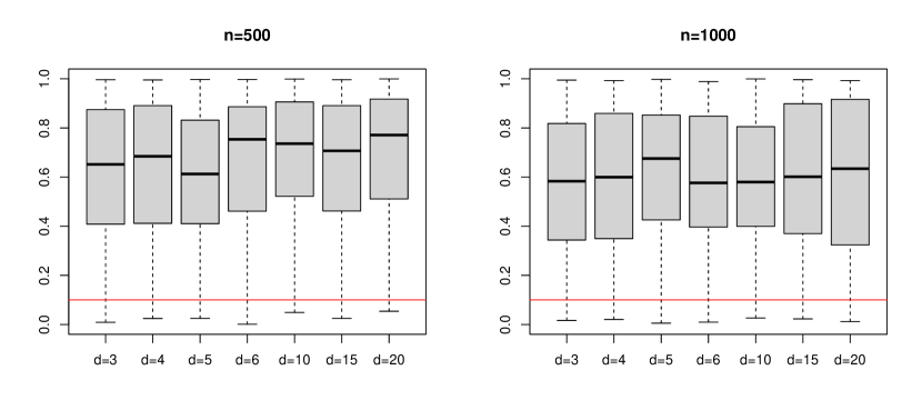
Figure 1: Boxplots of p-values under the null hypothesis. The red line represents 0.1.

As we can see the bulk of the p-values are quite large for all combinations of $n$ and $d$, indicating the elliptical distribution hypothesis is not rejected in the great majority of cases.

7.2 Results under alternative distributions

We consider alternative distributions with different degrees of departure from the elliptical distribution. We first generate $Z_{\scriptscriptstyle{k}}$ independently from $N(0,4)$, and set $Z=(Z_{\scriptscriptstyle{1}},\ldots,Z_{\scriptscriptstyle{d}})^{\mbox{\tiny{\sf T}}}$. We then randomly select a subset $J$ of $\{1,\ldots,d\}$ of cardinality $\lceil d/3\rceil$ and, for each $k\in J$, we replace $Z_{\scriptscriptstyle{k}}$ by $W_{\scriptscriptstyle{k}}-df$, with $W_{\scriptscriptstyle{k}}$ generated from $\chi^{\scriptscriptstyle{2}}(df)$. We denote the resulting random vector by $\tilde{Z}$. We then construct $X$ by

$$X=\mu+\Sigma^{\scriptscriptstyle{1/2}}\tilde{Z},$$

where $\Sigma$ is generated in the same way as it was in the null distribution case, and $\mu=(\mu_{\scriptscriptstyle{1}},\ldots,\mu_{\scriptscriptstyle{d}})^{\mbox{\tiny{\sf T}}}$ is generated from

$$\mu_{\scriptscriptstyle{k}}=40\beta_{\scriptscriptstyle{k}}-20,\quad k=1,\ldots,d,$$

where each $\beta_{\scriptscriptstyle{k}}$ is independently generated from $\mathrm{Beta}(0.5,0.5)$. That is, each $\mu_{\scriptscriptstyle{k}}$ is a rescaled and centered Beta variable. We take the degrees of freedom $df$ to be $2$ or $4$, with $df=2$ representing stronger departure from ellipticity.

We then perform our proposed test on the i.i.d. samples $X_{\scriptscriptstyle{1}},\ldots,X_{\scriptscriptstyle{n}}$ from $X$. The boxplots in Figure 2 show p-values for $df=4$ with $(n,d)$ in the range (7.1); those in Figure 3 show p-values for $df=2$ with $(n,d)$ in the same range.

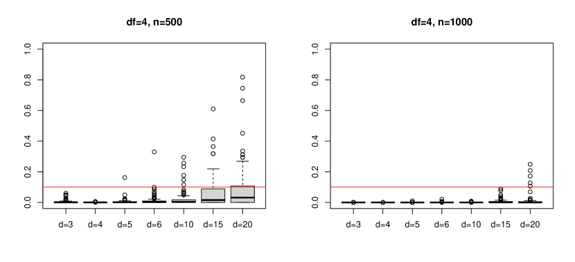
Figure 2: Boxplots of p-values under the alternative hypothesis with $df=4$. The red line represents 0.1.

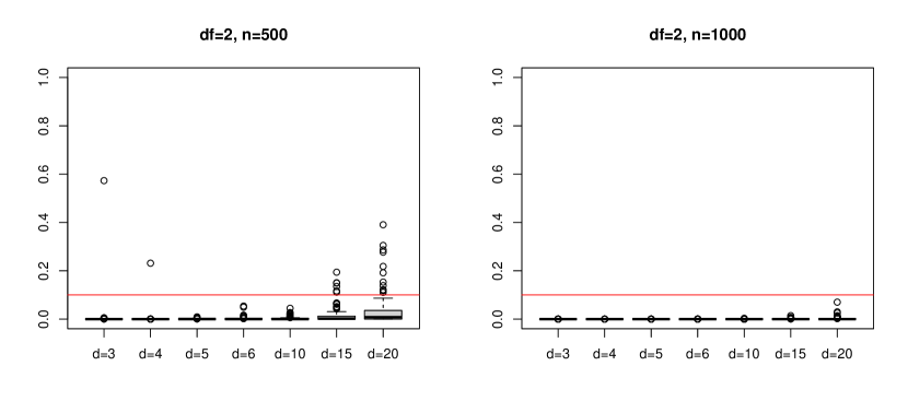
Figure 3: Boxplots of p-values under the alternative hypothesis with $df=2$. The red line represents 0.1.

According to Figure 2 and Figure 3, the bulk of the p-values are smaller than 0.1, indicating strong evidence that $X$ does not have an elliptical distribution. This implies the consistency of our test. More specifically, in each figure, when the sample size $n$ is fixed, the boxplots becomes slightly higher as $d$ increases, indicating it is more difficult to detect non-ellipticity in higher dimensions. This is reasonable because the skewness might be masked by higher dimensions. If we fix the dimension $d$ and the skewness as represented by $df$, an increase of sample size $n$ from 500 to 1000 makes the p-values more concentrated around 0. Furthermore, comparing Figure 3 with Figure 2, we see that the p-values for $df=2$ are smaller than those for $df=4$, indicating that an increase of skewness makes non-ellipticity more detectable.

7.3 Comparisons to existing methods

We also compare our test with the tests in Albisetti, Balabdaoui and Holzmann (2020) and Huffer and Park (2007) described in the Introduction, as they are the ones that test ellipticity without imposing any restrictions on alternative distributions. Both methods are based on bootstrap and, in applying both of them, we first need to standardize the dataset by the sample mean vector and the sample covariance matrix. We compare the three methods both in their powers and in their computing times. We refer to our proposed test as KEPT, short-hand for “kernel-embedding-of-probability test”.

The test proposed by Albisetti, Balabdaoui and Holzmann (2020) is based on a Kolmogorov-Smirnov statistic, which is the supremum norm of the empirical process over a specific class of functions. To compute the test statistic, we use the discretization method proposed in that paper, where we randomly generate an index set of the function class and maximize the absolute value of the norm of the empirical process over the finite set of functions. The finite set contains $N_{\scriptscriptstyle{u}}^{\scriptscriptstyle{2}}(N_{\scriptscriptstyle{c}}+1)$ functions, where $N_{\scriptscriptstyle{u}}$ and $N_{\scriptscriptstyle{c}}$ are fixed integers. The procedure also involves a truncation constant $c_{\scriptscriptstyle{0}}$. We use bootstrap to construct the reference distribution with bootstrap sample size $B=100$. We take $N_{\scriptscriptstyle{u}}=50$, $N_{\scriptscriptstyle{c}}=50$ and $c_{\scriptscriptstyle{0}}=10$ in our simulations to keep the running time in a manageable range. Since the computing of the test statistic is very time-consuming, the constants $N_{\scriptscriptstyle{u}}$ and $N_{\scriptscriptstyle{c}}$ are much smaller than the ones used in Albisetti, Balabdaoui and Holzmann (2020). We refer to this method as the b-KS, abbreviation for “bootstrap Kolmogorov-Smirnov test”.

The test proposed by Huffer and Park (2007) is based on the Pearson’s chi-square statistic after slicing the dataset into $gc$ cells, where $g$ refers to the number of sectors based on the directional vector and $c$ refers to the number of cells divided by the equally-spaced empirical quantiles of the length. Same as Huffer and Park (2007), we $g=2^{\scriptscriptstyle{d}}$ and $c=3$. We compute the chi-square statistic $X^{\scriptscriptstyle{2}}$ based on the cell counts. Since we do not assume that the distribution is similar to the multivariate normal distribution, we use bootstrap rather than the asymptotic distribution Huffer and Park (2007) provides under the multivariate normal assumption. We set the bootstrap sample size $B=100$. We refer to this method as the b-chi, abbreviation for “bootstrap chi-square test”.

We use $n=200$ and $d=3,6,10$ to make comparisons on the three methods. The null distribution case is same as that in Section 7.1, and the alternative distribution cases are the same as the two cases in Section 7.2. The boxplots of p-values for the null distribution are shown as Figure 4.

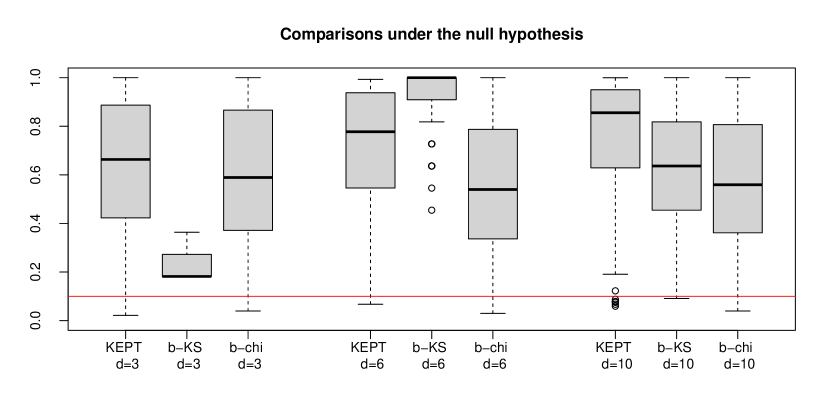
Figure 4: Boxplots of p-values under the null distribution using the three methods: “KEPT”, which refers to the proposed kernel-embedding-of-probability test, “b-KS”, which refers to the bootstrap Kolmogorov-Smirnov test, and “b-chi”, which refers to the bootstrap chi-square test. The red line represents 0.1.

According to Figure 4, the bulk of the p-values are quite large for all three tests and for all dimensions, indicating the elliptical distribution hypothesis is not rejected in the great majority of cases. However, we notice the b-KS test varies a lot with different dimensions, possibly because we use much smaller values of $N_{\scriptscriptstyle{u}}$ and $N_{\scriptscriptstyle{c}}$ than Albisetti, Balabdaoui and Holzmann (2020) to keep down the computing time.

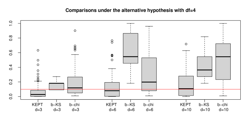
Figure 5: Boxplots of p-values under the alternative distributions with $df=4$ using the three methods: “KEPT”, which refers to the proposed kernel-embedding-of-probability test, “b-KS”, which refers to the bootstrap Kolmogorov-Smirnov test, and “b-chi”, which refers to the bootstrap chi-square test. The red line represents 0.1.

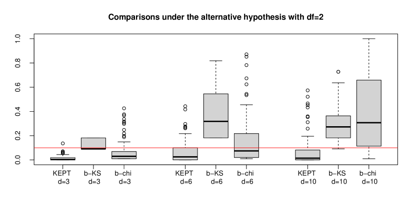
Figure 6: Boxplots of p-values under the alternative distributions with $df=2$ using the three methods: “KEPT”, which refers to the proposed kernel-embedding-of-probability test, “b-KS”, which refers to the bootstrap Kolmogorov-Smirnov test, and “b-chi”, which refers to the bootstrap chi-square test. The red line represents 0.1.

For the alternative distributions, the boxplots of p-values under different dimensions and for different tests are shown in Figure 5 for $df=4$ and in Figure 6 for $df=2$. Figure 5 and Figure 6 both indicate that our proposed KEPT gives the lowest p-values among the three tests under different dimensions and different alternative distributions, which confirms the power of our proposed test. We again observe a large variation in the b-KS test, which can also be attributed to the small values of $N_{\scriptscriptstyle{u}}$ and $N_{\scriptscriptstyle{c}}$. The power of the b-chi statistic is much lower than KEPT, possibly because the slicing step loses some information in the skewness.

We also compare the running times of the three methods under different dimensions. The average user CPU times are presented as Table 1, which shows that, in general, the running time of b-chi is the lowest, followed by KEPT, and then by b-KS by a large gap. Specifically, b-KS requires more than an hour to compute for each dimension; whereas the other two methods require less than 30 seconds.

Table 1: Average user CPU time (in seconds) for the three methods.

	$d=3$	$d=6$	$d=10$
KEPT	5.7281	11.8558	29.8941
b-KS	5037.5532	5047.4248	5093.8702
b-chi	0.6556	0.8272	1.0968

8 Application

In this section we apply our test to a dataset concerning a Study on the Efficacy of Nosocomial Infection Control (SENIC Project), which is used in Haley et al. (1980). We download the dataset from https://users.stat.ufl.edu/~rrandles/sta4210/Rclassnotes/data/textdatasets/KutnerData/Appendix%20C%20Data%20Sets/APPENC01.txt. This is one of the datasets from the book Kutner et al. (2005).

According to Kutner et al. (2005), the data of 113 hospitals during the 1975-76 study period are sampled from the original 338 hospitals surveyed. For a single hospital, there are 11 variables:

length of stay, age, infection risk, routine culturing, routine chest x-ray, number of beds, medical school affiliation, region, average daily census, number of nurses, available facilities.

For detailed information about these variables, see Kutner et al. (2005).

We treat the variable “length of stay” as the response variable, and check whether other predictor variables are elliptically distributed. We remove the two categorical variables, “medical school affiliation” and “region”. We carry out our test on the dataset where $n=113$ and $d=8$ at a significance level $\alpha=0.05$, and obtained the p-value 0.0014, which leads to rejection of the elliptical distribution hypothesis. The original data is as Figure 1 in Appendix B of the online Supplementary Material (Tang and Li (2023)).

We then perform the Box-Cox transformation on the dataset. Using the method presented in Chapter 7 of Li (2018), we find the optimal $\lambda$ for the Box-Cox transformation as

$$1.158,0.737,-0.105,0.947,-0.316,-0.105,-0.316,0.947.$$

The transformed variables are shown in Figure 2 in Appendix B of the online Supplementary Material (Tang and Li (2023)). We carry out our test on the transformed data, and obtain the p-value 0.2454. This is much larger than 0.05, leading us to accept the elliptical distribution hypothesis after the Box-Cox transformation.

The research of Bing Li is supported in part by the U.S. National Science Foundation Grant DMS-2210775.

Supplementary material for “A nonparametric test for elliptical distribution based on kernel embedding of probabilities” Additional proofs in this paper and the scatter plot matrices in Section 8 can be found in the Supplementary Material.

References

• Albisetti, Balabdaoui and Holzmann (2020) {barticle}[author] \bauthor\bsnmAlbisetti, \bfnmIsaia\binitsI., \bauthor\bsnmBalabdaoui, \bfnmFadoua\binitsF. and \bauthor\bsnmHolzmann, \bfnmHajo\binitsH. (\byear2020). \btitleTesting for spherical and elliptical symmetry. \bjournalJournal of Multivariate Analysis \bvolume180 \bpages104667. \bdoihttps://doi.org/10.1016/j.jmva.2020.104667 \endbibitem
• Anderson (2003) {bbook}[author] \bauthor\bsnmAnderson, \bfnmT. W.\binitsT. W. (\byear2003). \btitleAn Introduction to Multivariate Statistical Analysis. \bpublisherJohn Wiley & Suns, Inc. Huboken, New Jersey. \endbibitem
• Babic et al. (2019) {bmisc}[author] \bauthor\bsnmBabic, \bfnmSladana\binitsS., \bauthor\bsnmGelbgras, \bfnmLaetitia\binitsL., \bauthor\bsnmHallin, \bfnmMarc\binitsM. and \bauthor\bsnmLey, \bfnmChristophe\binitsC. (\byear2019). \btitleOptimal tests for elliptical symmetry: specified and unspecified location. \endbibitem
• Baringhaus (1991) {barticle}[author] \bauthor\bsnmBaringhaus, \bfnmLudwig\binitsL. (\byear1991). \btitleTesting for Spherical Symmetry of a Multivariate Distribution. \bjournalThe Annals of Statistics \bvolume19 \bpages899–917. \endbibitem
• Cambanis, Huang and Simons (1981) {barticle}[author] \bauthor\bsnmCambanis, \bfnmStamatis\binitsS., \bauthor\bsnmHuang, \bfnmSteel\binitsS. and \bauthor\bsnmSimons, \bfnmGordon\binitsG. (\byear1981). \btitleOn the theory of elliptically contoured distributions. \bjournalJournal of Multivariate Analysis \bvolume11 \bpages368-385. \bdoihttps://doi.org/10.1016/0047-259X(81)90082-8 \endbibitem
• Cook and Li (2002) {barticle}[author] \bauthor\bsnmCook, \bfnmR Dennis\binitsR. D. and \bauthor\bsnmLi, \bfnmBing\binitsB. (\byear2002). \btitleDimension Reduction for Conditional Mean in Regression. \bjournalThe Annals of Statistics \bvolume30 \bpages455–474. \endbibitem
• Duchesne and de Micheaux (2010) {barticle}[author] \bauthor\bsnmDuchesne, \bfnmP.\binitsP. and \bauthor\bsnmde Micheaux, \bfnmP. Lafaye\binitsP. L. (\byear2010). \btitleComputing the distribution of quadratic forms: Further comparisons between the Liu-Tang-Zhang approximation and exact methods. \bjournalComputational Statistics and Data Analysis \bvolume54 \bpages858-862. \endbibitem
• Eaton (1986) {barticle}[author] \bauthor\bsnmEaton, \bfnmMorris L\binitsM. L. (\byear1986). \btitleA characterization of spherical distributions. \bjournalJournal of Multivariate Analysis \bvolume20 \bpages272–276. \endbibitem
• Fernholz (1983) {binproceedings}[author] \bauthor\bsnmFernholz, \bfnmLuisa T.\binitsL. T. (\byear1983). \btitlevon Mises Calculus For Statistical Functionals. \endbibitem
• Fukumizu et al. (2009) {binproceedings}[author] \bauthor\bsnmFukumizu, \bfnmKenji\binitsK., \bauthor\bsnmGretton, \bfnmArthur\binitsA., \bauthor\bsnmLanckriet, \bfnmGert\binitsG., \bauthor\bsnmSchölkopf, \bfnmBernhard\binitsB. and \bauthor\bsnmSriperumbudur, \bfnmBharath K.\binitsB. K. (\byear2009). \btitleKernel Choice and Classifiability for RKHS Embeddings of Probability Distributions. In \bbooktitleAdvances in Neural Information Processing Systems (\beditor\bfnmY.\binitsY. \bsnmBengio, \beditor\bfnmD.\binitsD. \bsnmSchuurmans, \beditor\bfnmJ.\binitsJ. \bsnmLafferty, \beditor\bfnmC.\binitsC. \bsnmWilliams and \beditor\bfnmA.\binitsA. \bsnmCulotta, eds.) \bvolume22. \bpublisherCurran Associates, Inc. \endbibitem
• Gretton et al. (2005) {binproceedings}[author] \bauthor\bsnmGretton, \bfnmArthur\binitsA., \bauthor\bsnmBousquet, \bfnmOlivier\binitsO., \bauthor\bsnmSmola, \bfnmAlex\binitsA. and \bauthor\bsnmSchölkopf, \bfnmBernhard\binitsB. (\byear2005). \btitleMeasuring Statistical Dependence with Hilbert-Schmidt Norms. In \bbooktitleAlgorithmic Learning Theory (\beditor\bfnmSanjay\binitsS. \bsnmJain, \beditor\bfnmHans Ulrich\binitsH. U. \bsnmSimon and \beditor\bfnmEtsuji\binitsE. \bsnmTomita, eds.) \bpages63–77. \bpublisherSpringer Berlin Heidelberg, \baddressBerlin, Heidelberg. \endbibitem
• Gretton et al. (2007) {binproceedings}[author] \bauthor\bsnmGretton, \bfnmArthur\binitsA., \bauthor\bsnmBorgwardt, \bfnmKarsten M. \binitsK., \bauthor\bsnmRasch, \bfnmMalte Johannes\binitsM., \bauthor\bsnmSchoelkopf, \bfnmBernhard\binitsB. and \bauthor\bsnmSmola, \bfnmAlex J. \binitsA. (\byear2007). \btitleA kernel method for the two-sample-problem. In \bbooktitleAdvances in neural information processing systems 19 \bpages513–520. \bpublisher. \bnote20th Annual Conference on Neural Information Processing Systems : NIPS 2006 ; Conference date: 04-12-2006 Through 07-12-2006. \endbibitem
• Gretton et al. (2008) {binproceedings}[author] \bauthor\bsnmGretton, \bfnmArthur\binitsA., \bauthor\bsnmFukumizu, \bfnmKenji\binitsK., \bauthor\bsnmTeo, \bfnmChoon\binitsC., \bauthor\bsnmSong, \bfnmLe\binitsL., \bauthor\bsnmSchölkopf, \bfnmBernhard\binitsB. and \bauthor\bsnmSmola, \bfnmAlex\binitsA. (\byear2008). \btitleA Kernel Statistical Test of Independence. In \bbooktitleAdvances in Neural Information Processing Systems (\beditor\bfnmJ.\binitsJ. \bsnmPlatt, \beditor\bfnmD.\binitsD. \bsnmKoller, \beditor\bfnmY.\binitsY. \bsnmSinger and \beditor\bfnmS.\binitsS. \bsnmRoweis, eds.) \bvolume20. \bpublisherCurran Associates, Inc. \endbibitem
• Gretton et al. (2009) {binproceedings}[author] \bauthor\bsnmGretton, \bfnmArthur\binitsA., \bauthor\bsnmFukumizu, \bfnmKenji\binitsK., \bauthor\bsnmHarchaoui, \bfnmZaïd\binitsZ. and \bauthor\bsnmSriperumbudur, \bfnmBharath K.\binitsB. K. (\byear2009). \btitleA Fast, Consistent Kernel Two-Sample Test. In \bbooktitleAdvances in Neural Information Processing Systems (\beditor\bfnmY.\binitsY. \bsnmBengio, \beditor\bfnmD.\binitsD. \bsnmSchuurmans, \beditor\bfnmJ.\binitsJ. \bsnmLafferty, \beditor\bfnmC.\binitsC. \bsnmWilliams and \beditor\bfnmA.\binitsA. \bsnmCulotta, eds.) \bvolume22. \bpublisherCurran Associates, Inc. \endbibitem
• Gretton et al. (2012) {barticle}[author] \bauthor\bsnmGretton, \bfnmArthur\binitsA., \bauthor\bsnmBorgwardt, \bfnmKarsten M.\binitsK. M., \bauthor\bsnmRasch, \bfnmMalte J.\binitsM. J., \bauthor\bsnmSchölkopf, \bfnmBernhard\binitsB. and \bauthor\bsnmSmola, \bfnmAlex\binitsA. (\byear2012). \btitleA Kernel Two-Sample Test. \bjournalJ. Mach. Learn. Res. \bvolume13 \bpages723-773. \endbibitem
• Guella (2021) {bmisc}[author] \bauthor\bsnmGuella, \bfnmJean Carlo\binitsJ. C. (\byear2021). \btitleOn Gaussian kernels on Hilbert spaces and kernels on Hyperbolic spaces. \endbibitem
• Haley et al. (1980) {barticle}[author] \bauthor\bsnmHaley, \bfnmRobert W.\binitsR. W., \bauthor\bsnmQuade, \bfnmDana\binitsD., \bauthor\bsnmFreeman, \bfnmHoward E.\binitsH. E. and \bauthor\bsnmBennett, \bfnmJohn V.\binitsJ. V. (\byear1980). \btitleThe SENIC Project. Study on the efficacy of nosocomial infection control (SENIC Project). Summary of study design. \bjournalAmerican Journal of Epidemiology \bvolume111 \bpages472-485. \bdoi10.1093/oxfordjournals.aje.a112928 \endbibitem
• Henze, Hlávka and Meintanis (2014) {barticle}[author] \bauthor\bsnmHenze, \bfnmN.\binitsN., \bauthor\bsnmHlávka, \bfnmZ.\binitsZ. and \bauthor\bsnmMeintanis, \bfnmS. G.\binitsS. G. (\byear2014). \btitleTesting for spherical symmetry via the empirical characteristic function. \bjournalStatistics \bvolume48 \bpages1282-1296. \bdoi10.1080/02331888.2013.832764 \endbibitem
• Huffer and Park (2007) {barticle}[author] \bauthor\bsnmHuffer, \bfnmFred W.\binitsF. W. and \bauthor\bsnmPark, \bfnmCheolyong\binitsC. (\byear2007). \btitleA test for elliptical symmetry. \bjournalJournal of Multivariate Analysis \bvolume98 \bpages256-281. \bdoihttps://doi.org/10.1016/j.jmva.2005.09.011 \endbibitem
• Kariya and Eaton (1977) {barticle}[author] \bauthor\bsnmKariya, \bfnmTakeaki\binitsT. and \bauthor\bsnmEaton, \bfnmMorris L.\binitsM. L. (\byear1977). \btitleRobust Tests for Spherical Symmetry. \bjournalThe Annals of Statistics \bvolume5 \bpages206–215. \endbibitem
• Kokoszka and Reimherr (2017) {bbook}[author] \bauthor\bsnmKokoszka, \bfnmP.\binitsP. and \bauthor\bsnmReimherr, \bfnmM.\binitsM. (\byear2017). \btitleIntroduction to Functional Data Analysis. \bseriesChapman & Hall/CRC Texts in Statistical Science. \bpublisherCRC Press. \endbibitem
• Koltchinskii and Li (1998) {barticle}[author] \bauthor\bsnmKoltchinskii, \bfnmV. I.\binitsV. I. and \bauthor\bsnmLi, \bfnmLang\binitsL. (\byear1998). \btitleTesting for Spherical Symmetry of a Multivariate Distribution. \bjournalJournal of Multivariate Analysis \bvolume65 \bpages228-244. \bdoihttps://doi.org/10.1006/jmva.1998.1743 \endbibitem
• Kutner et al. (2005) {bbook}[author] \bauthor\bsnmKutner, \bfnmMichael\binitsM., \bauthor\bsnmNachtsheim, \bfnmChristopher\binitsC., \bauthor\bsnmNeter, \bfnmJohn\binitsJ. and \bauthor\bsnmLi, \bfnmWilliam\binitsW. (\byear2005). \btitleApplied Linear Statistical Models. \bseriesMcGrwa-Hill international edition. \bpublisherMcGraw-Hill Irwin. \endbibitem
• Li (1991) {barticle}[author] \bauthor\bsnmLi, \bfnmKer-Chau\binitsK.-C. (\byear1991). \btitleSliced Inverse Regression for Dimension Reduction. \bjournalJournal of the American Statistical Association \bvolume86 \bpages316–327. \endbibitem
• Li (2018) {bbook}[author] \bauthor\bsnmLi, \bfnmB.\binitsB. (\byear2018). \btitleSufficient Dimension Reduction: Methods and Applications with R. \bseriesChapman & Hall/CRC Monographs on Statistics and Applied Probability. \bpublisherCRC Press. \endbibitem
• Li and Dong (2009) {barticle}[author] \bauthor\bsnmLi, \bfnmBing\binitsB. and \bauthor\bsnmDong, \bfnmYuexiao\binitsY. (\byear2009). \btitleDimension reduction for nonelliptically distributed predictors. \bjournalThe Annals of Statistics \bvolume37 \bpages1272 – 1298. \bdoi10.1214/08-AOS598 \endbibitem
• Li and Duan (1989) {barticle}[author] \bauthor\bsnmLi, \bfnmKer-Chau\binitsK.-C. and \bauthor\bsnmDuan, \bfnmNaihua\binitsN. (\byear1989). \btitleRegression Analysis Under Link Violation. \bjournalThe Annals of Statistics \bvolume17 \bpages1009 – 1052. \bdoi10.1214/aos/1176347254 \endbibitem
• Li and Solea (2018) {barticle}[author] \bauthor\bsnmLi, \bfnmBing\binitsB. and \bauthor\bsnmSolea, \bfnmEftychia\binitsE. (\byear2018). \btitleA Nonparametric Graphical Model for Functional Data With Application to Brain Networks Based on fMRI. \bjournalJournal of the American Statistical Association \bvolume113 \bpages1637-1655. \bdoi10.1080/01621459.2017.1356726 \endbibitem
• Liang, Fang and Hickernell (2008) {barticle}[author] \bauthor\bsnmLiang, \bfnmJiajuan\binitsJ., \bauthor\bsnmFang, \bfnmKai-Tai\binitsK.-T. and \bauthor\bsnmHickernell, \bfnmFred J.\binitsF. J. (\byear2008). \btitleSome necessary uniform tests for spherical symmetry. \bjournalAnnals of the Institute of Statistical Mathematics \bvolume60 \bpages679–696. \bdoi10.1007/s10463-007-0121-9 \endbibitem
• Liu, Han and Zhang (2012) {binproceedings}[author] \bauthor\bsnmLiu, \bfnmHan\binitsH., \bauthor\bsnmHan, \bfnmFang\binitsF. and \bauthor\bsnmZhang, \bfnmCun-Hui\binitsC.-H. (\byear2012). \btitleTranselliptical Graphical Models. In \bbooktitleNIPS \bpages809-817. \endbibitem
• Manzotti, Pérez and Quiroz (2002) {barticle}[author] \bauthor\bsnmManzotti, \bfnmA.\binitsA., \bauthor\bsnmPérez, \bfnmFrancisco J.\binitsF. J. and \bauthor\bsnmQuiroz, \bfnmAdolfo J.\binitsA. J. (\byear2002). \btitleA Statistic for Testing the Null Hypothesis of Elliptical Symmetry. \bjournalJournal of Multivariate Analysis \bvolume81 \bpages274-285. \bdoihttps://doi.org/10.1006/jmva.2001.2007 \endbibitem
• Narasimhan et al. (2023) {bmanual}[author] \bauthor\bsnmNarasimhan, \bfnmBalasubramanian\binitsB., \bauthor\bsnmJohnson, \bfnmSteven G.\binitsS. G., \bauthor\bsnmHahn, \bfnmThomas\binitsT., \bauthor\bsnmBouvier, \bfnmAnnie\binitsA. and \bauthor\bsnmKiêu, \bfnmKiên\binitsK. (\byear2023). \btitlecubature: Adaptive Multivariate Integration over Hypercubes \bnoteR package version 2.0.4.6. \endbibitem
• Qiu and Joe. (2020) {bmanual}[author] \bauthor\bsnmQiu, \bfnmWeiliang\binitsW. and \bauthor\bsnmJoe., \bfnmHarry\binitsH. (\byear2020). \btitleclusterGeneration: Random Cluster Generation (with Specified Degree of Separation) \bnoteR package version 1.3.7. \endbibitem
• Schmidt (2002) {barticle}[author] \bauthor\bsnmSchmidt, \bfnmRafael\binitsR. (\byear2002). \btitleTail dependence for elliptically contoured distributions. \bjournalMathematical Methods of Operations Research \bvolume55 \bpages301-327. \bdoi10.1007/s001860200191 \endbibitem
• Schölkopf, Herbrich and Smola (2001) {binproceedings}[author] \bauthor\bsnmSchölkopf, \bfnmBernhard\binitsB., \bauthor\bsnmHerbrich, \bfnmRalf\binitsR. and \bauthor\bsnmSmola, \bfnmAlex J.\binitsA. J. (\byear2001). \btitleA Generalized Representer Theorem. In \bbooktitleComputational Learning Theory (\beditor\bfnmDavid\binitsD. \bsnmHelmbold and \beditor\bfnmBob\binitsB. \bsnmWilliamson, eds.) \bpages416–426. \bpublisherSpringer Berlin Heidelberg, \baddressBerlin, Heidelberg. \endbibitem
• Sejdinovic et al. (2013) {barticle}[author] \bauthor\bsnmSejdinovic, \bfnmDino\binitsD., \bauthor\bsnmSriperumbudur, \bfnmBharath\binitsB., \bauthor\bsnmGretton, \bfnmArthur\binitsA. and \bauthor\bsnmFukumizu, \bfnmKenji\binitsK. (\byear2013). \btitleEquivalence of Distance-Based and RKHS-Based Statistics in Hypothesis Testing. \bjournalThe Annals of Statistics \bvolume41 \bpages2263–2291. \endbibitem
• Sriperumbudur, Fukumizu and Lanckriet (2010) {binproceedings}[author] \bauthor\bsnmSriperumbudur, \bfnmBharath\binitsB., \bauthor\bsnmFukumizu, \bfnmKenji\binitsK. and \bauthor\bsnmLanckriet, \bfnmGert\binitsG. (\byear2010). \btitleOn the relation between universality, characteristic kernels and RKHS embedding of measures. In \bbooktitleProceedings of the Thirteenth International Conference on Artificial Intelligence and Statistics (\beditor\bfnmYee Whye\binitsY. W. \bsnmTeh and \beditor\bfnmMike\binitsM. \bsnmTitterington, eds.). \bseriesProceedings of Machine Learning Research \bvolume9 \bpages773–780. \bpublisherPMLR, \baddressChia Laguna Resort, Sardinia, Italy. \endbibitem
• Sriperumbudur, Fukumizu and Lanckriet (2011) {barticle}[author] \bauthor\bsnmSriperumbudur, \bfnmBharath K.\binitsB. K., \bauthor\bsnmFukumizu, \bfnmKenji\binitsK. and \bauthor\bsnmLanckriet, \bfnmGert R. G.\binitsG. R. G. (\byear2011). \btitleUniversality, Characteristic Kernels and RKHS Embedding of Measures. \bjournalJournal of Machine Learning Research \bvolume12 \bpages2389–2410. \endbibitem
• Sriperumbudur et al. (2010) {barticle}[author] \bauthor\bsnmSriperumbudur, \bfnmBK.\binitsB., \bauthor\bsnmGretton, \bfnmA.\binitsA., \bauthor\bsnmFukumizu, \bfnmK.\binitsK., \bauthor\bsnmSchölkopf, \bfnmB.\binitsB. and \bauthor\bsnmLanckriet, \bfnmGRG.\binitsG. (\byear2010). \btitleHilbert Space Embeddings and Metrics on Probability Measures. \bjournalJournal of Machine Learning Research \bvolume11 \bpages1517-1561. \endbibitem
• Szabó and Sriperumbudur (2018) {barticle}[author] \bauthor\bsnmSzabó, \bfnmZoltán\binitsZ. and \bauthor\bsnmSriperumbudur, \bfnmBharath K.\binitsB. K. (\byear2018). \btitleCharacteristic and Universal Tensor Product Kernels. \bjournalJournal of Machine Learning Research \bvolume18 \bpages1–29. \endbibitem
• Székely, Rizzo and Bakirov (2007) {barticle}[author] \bauthor\bsnmSzékely, \bfnmGábor J.\binitsG. J., \bauthor\bsnmRizzo, \bfnmMaria L.\binitsM. L. and \bauthor\bsnmBakirov, \bfnmNail K.\binitsN. K. (\byear2007). \btitleMeasuring and testing dependence by correlation of distances. \bjournalThe Annals of Statistics \bvolume35 \bpages2769 – 2794. \bdoi10.1214/009053607000000505 \endbibitem
• Székely and Rizzo (2009) {barticle}[author] \bauthor\bsnmSzékely, \bfnmGábor J.\binitsG. J. and \bauthor\bsnmRizzo, \bfnmMaria L.\binitsM. L. (\byear2009). \btitleBrownian distance covariance. \bjournalThe Annals of Applied Statistics \bvolume3 \bpages1236 – 1265. \bdoi10.1214/09-AOAS312 \endbibitem
• Tang and Li (2023) {barticle}[author] \bauthor\bsnmTang, \bfnmYin\binitsY. and \bauthor\bsnmLi, \bfnmBing\binitsB. (\byear2023). \btitleSupplementary material for “A nonparametric test for elliptical distribution based on kernel embedding of probabilities”. \endbibitem
• Vaart (1998) {bbook}[author] \bauthor\bsnmVaart, \bfnmA. W. van der\binitsA. W. v. d. (\byear1998). \btitleAsymptotic Statistics. \bseriesCambridge Series in Statistical and Probabilistic Mathematics. \bpublisherCambridge University Press. \bdoi10.1017/CBO9780511802256 \endbibitem
• Vogel and Fried (2011) {barticle}[author] \bauthor\bsnmVogel, \bfnmD.\binitsD. and \bauthor\bsnmFried, \bfnmR.\binitsR. (\byear2011). \btitleElliptical graphical modelling. \bjournalBiometrika \bvolume98 \bpages935–951. \endbibitem
• Yuan and Lin (2006) {barticle}[author] \bauthor\bsnmYuan, \bfnmMing\binitsM. and \bauthor\bsnmLin, \bfnmYi\binitsY. (\byear2006). \btitleModel selection and estimation in regression with grouped variables. \bjournalJournal of the Royal Statistical Society: Series B (Statistical Methodology) \bvolume68 \bpages49–67. \endbibitem
• Zhou (2008) {barticle}[author] \bauthor\bsnmZhou, \bfnmDing-Xuan\binitsD.-X. (\byear2008). \btitleDerivative reproducing properties for kernel methods in learning theory. \bjournalJournal of Computational and Applied Mathematics \bvolume220 \bpages456–463. \endbibitem