Machine Learning and Hamilton-Jacobi-Bellman Equation
for Optimal Decumulation: a Comparison Study

Abstract

We propose a novel data-driven neural network (NN) optimization framework for solving an optimal stochastic control problem under stochastic constraints. Customized activation functions for the output layers of the NN are applied, which permits training via standard unconstrained optimization. The optimal solution yields a multi-period asset allocation and decumulation strategy for a holder of a defined contribution (DC) pension plan. The objective function of the optimal control problem is based on expected wealth withdrawn (EW) and expected shortfall (ES) that directly targets left-tail risk. The stochastic bound constraints enforce a guaranteed minimum withdrawal each year. We demonstrate that the data-driven approach is capable of learning a near-optimal solution by benchmarking it against the numerical results from a Hamilton-Jacobi-Bellman (HJB) Partial Differential Equation (PDE) computational framework.

Keywords: Portfolio decumulation, neural network, stochastic optimal control

JEL codes: G11, G22
AMS codes: 93E20, 91G, 68T07, 65N06, 35Q93

1 Introduction

Access to traditional defined benefit (DB) pension plans continues to disappear for employees. In 2022, only 15% of private sector workers in the United States had access to a defined benefit plan, while 66% had access to a defined contribution (DC) plan (U.S. Bureau of Labor Statistics, 2022). In other countries, DB plans have become a thing of the past.

Defined contribution plans leave the burden of creating an investment and withdrawal strategy to the individual investor, which Nobel Laureate William Sharpe referred to as “the nastiest, hardest problem in finance” (Ritholz, 2017). Indeed, a review of the literature on decumulation strategies (Bernhardt and Donnelly, 2018; MacDonald et al., 2013) shows that balancing all of retirees’ concerns with a single strategy is exceedingly difficult. To address these concerns and find an optimal balance between maximizing withdrawals and minimizing the risk of depletion, while guaranteeing a minimum withdrawal, the approach in Forsyth (2022) determines a decumulation and allocation strategy for a standard 30-year investment horizon by formulating it as a problem in optimal stochastic control. Numerical solutions are obtained using dynamic programming, which results in a Hamilton-Jacobi-Bellman (HJB) Partial Differential Equation (PDE).

The HJB PDE framework developed in Forsyth (2022) maximizes expected withdrawals and minimizes the risk of running out of savings, measured by the left-tail in the terminal wealth distribution. Since maximizing withdrawals and minimizing risk are conflicting measures, we use a scalarization technique to compute Pareto optimal points. A constant lower bound is imposed on the withdrawal, providing a guaranteed income. An upper bound on withdrawal is also imposed, which can be viewed as the target withdrawal. The constraints of no shorting and no leverage are imposed on the investment allocation.

The solution to this constrained stochastic optimal control problem yields a dynamic stochastic strategy, naturally aligning with retirees’ concerns and objectives. Note that cash flows are not mortality weighted, consistent with Bengen (1994). This can be justified on the basis of planning to live, not planning to die as discussed in Pfau (2018).

Our dynamic strategy can be contrasted to traditional strategies such as the Bengen Rule (4% Rule), which recommends withdrawing a constant 4% of initial capital each year (adjusted for inflation) and investing equal amounts into stocks and bonds (Bengen, 1994). Initially proposed in 1994, Scott et al. (2009) found the 4% Rule to still be a popular strategy 14 years later, and the near-universal recommendation of the top brokerage and retirement planning groups. Recently there has been acknowledgment in the asset management industry that the 4% Rule is sub-optimal, but wealth managers still recommend variations of the same constant withdrawal principle (Williams and Kawashima, 2023). The strategy proposed by Forsyth (2022) is shown to be far more efficient than the Bengen 4% Rule. Of course, the PDE solution in Forsyth (2022) is restricted to low dimensions (i.e. a small number of stochastic factors).

In order to remedy some of the deficiencies of PDE methods (such as in Forsyth (2022)), we propose a neural network (NN) based framework without using dynamic programming. In contrast to the PDE solution approach, our proposed NN approach has the following advantages:

1. It is data-driven and does not depend on a parametric model. This makes the framework versatile in selecting training data, and less susceptible to model misspecification.

2. The control is learned directly, thereby exploiting the low dimensionality of the control (van Staden et al., 2023). This technique thus avoids dynamic programming and the associated error propagation. The NN approach can also be applied to higher dimensional problems, such as those with a large number of assets.

3. If the control is a continuous function of time, the control approximated by the NN framework will reflect this property. If the control is discontinuous , the NN seems to produce a smooth, but quite accurate, approximation.

Since the NN only generates an approximate solution to the complex stochastic optimal control problem, it is essential to assess its accuracy and robustness. Rarely is the quality of an NN solution assessed rigorously, since an accurate solution to the optimal control problem is often not available. In this paper, we compare the NN solution to the decumulation problem against the ground-truth results from the provably convergent HJB PDE method.

We have previously seen such a comparison in different applications, see, e.g., Laurière et al. (2021) for a comparison study on a fishing control problem. As machine learning and artificial intelligence based methods continue to proliferate in finance and investment management, it is crucial to demonstrate that these methods are reliable and explainable (Boukherouaa et al., 2021). We believe that our proposed framework and test results make a step forward in demonstrating deep learning’s potential for stochastic control problems in finance.

To summarize, the main contributions of this paper are as follows:

• Proposing an NN framework with suitable activation functions for decumulation and allocation controls, which yields an approximate solution to the constrained stochastic optimal decumulation problem in Forsyth (2022) by solving a standard unconstrained optimization problem;

• Demonstrating that the NN solution achieves very high accuracy in terms of the efficient frontier and the decumulation control when compared to the solution from the provably convergent HJB PDE method;

• Illustrating that, with a suitably small regularization parameter, the NN allocation strategy can differ significantly from the PDE allocation strategy in the region of high wealth and near the terminal time, while the relevant performance statistics remain unaffected. This is due to the fact that the problem is ill-posed in these regions of the state space unless we add a small regularization term;

• Testing the NN solution’s robustness on out-of-sample and out-of-distribution data, as well as its versatility in using different datasets for training.

While other neural network and deep learning methods for optimal stochastic control problems have been proposed before, they differ significantly from our approach in their architecture, taking a stacked neural network approach as in Buehler et al. (2019); Han and E (2016); Tsang and Wong (2020) or a hybrid dynamic programming and reinforcement learning approach (Huré et al., 2021). On the other hand, our framework uses the same two neural networks at all rebalancing times in the investment scenario. Since our NNs take time as an input, the solution will be continuous in time if the control is continuous. Note that the idea of using time as an input to the NN was also suggested in Laurière et al. (2021). According to the taxonomy of sequential decision problems proposed in Powell (2021), our approach would most closely be described as Policy Function Approximation (PFA).

With the exception of Laurière et al. (2021), previous papers do not provide a benchmark for numerical methods, as we do in this work. Our results show that our proposed NN method is able to approximate the numerical results in Forsyth (2022) with high accuracy. Especially notable, and somewhat unexpected, is that the bang-bang control for the withdrawal is reproduced very closely with the NN method.

2 Problem Formulation

2.1 Overview

The investment scenario described in Forsyth (2022) concerns an investor with a portfolio wealth of a specified size, upon retirement. The investment horizon is fixed with a finite number of equally spaced rebalancing times (usually annually). At each rebalancing time, the investor first chooses how much to withdraw from the portfolio and then how to allocate the remaining wealth. The investor must withdraw an amount within a specified range. The wealth in this portfolio can be allocated to any mix of two given assets, with no shorting or leverage. The assets the investor can access are a broad stock index fund and a constant maturity bond index fund.

In the time that elapses between re-balancing times, the portfolio’s wealth will change according to the dynamics of the underlying assets. If the wealth of the portfolio goes below zero (due to minimum withdrawals), the portfolio is liquidated, trading ceases, debt accumulates at the borrowing rate, and withdrawals are restricted to the minimum amount. At the end of the time horizon, a final withdrawal is made and the portfolio is liquidated, yielding the terminal wealth.

We assume here that the investor has other assets, such as real estate, which are non-fungible with investment assets. These other assets can be regarded as a hedge of last resort, which can be used to fund any accumulated debt (Pfeiffer et al., 2013). This is not a novel assumption and is in line with the mental bucketing idea proposed by Shefrin and Thaler (1988). The use of this assumption within literature targeting similar problems is also common (see Forsyth et al. (2022)). Of course, the objective of the optimal control is to make running out of savings an unlikely event.

The investor’s goal then is to maximize the weighted sum of total withdrawals and the mean of the worst 5% of the outcomes (in terms of terminal wealth). We term this tail risk measure as Expected Shortfall (ES) at the 5% level. In this section, this optimization problem will be described with the mathematical details common to both the HJB and NN methods.

2.2 Stochastic Process Model

Let $S_{t}$ and $B_{t}$ represent the real (i.e. inflation-adjusted) amounts invested in the stock index and a constant maturity bond index, respectively. These assets are modeled with correlated jump diffusion models, in line with MacMinn et al. (2014). These parametric stochastic differential equations (SDEs) allow us to model non-normal asset returns. The SDEs are used in solving the HJB PDE, and generating training data with Monte Carlo simulations in the proposed NN framework. For the remainder of this paper, we refer to simulated data using these models as synthetic data.

When a jump occurs, $S_{t}=\xi^{s}S_{t^{-}}$, where $\xi^{s}$ is a random number representing the jump multiplier and $S_{t^{-}}=S(t-\epsilon),\epsilon\rightarrow 0^{+}$ ($S_{t^{-}}$ is the instant of time before $t$). We assume that $\log(\xi^{s})$ follows a double exponential distribution (Kou, 2002; Kou and Wang, 2004). The jump is either upward or downward, with probabilities $u^{s}$ and $1-u^{s}$ respectively. The density function for $y=\log(\xi^{s})$ is

$$f^{s}(y)=u^{s}\eta_{1}^{s}e^{-\eta_{1}^{s}y}{\bf{1}}_{y\geq 0}+(1-u^{s})\eta_{2}^{s}e^{\eta_{2}^{s}y}{\bf{1}}_{y<0}~{}.$$ (2.1)

We also define

$$\gamma^{s}_{\xi} = E[\xi^{s}-1]=\frac{u^{s}\eta_{1}^{s}}{\eta_{1}^{s}-1}+\frac{(1-u^{s})\eta_{2}^{s}}{\eta_{2}^{s}+1}-1~{}.$$ (2.2)

The starting point for building the jump diffusion model is a standard geometric Brownian motion, with drift rate $\mu^{s}$ and volatility $\sigma^{s}$. A third term is added to represent the effect of jumps, and a compensator is added to the drift term to preserve the expected drift rate. For stocks, this gives the following stochastic differential equation (SDE) that describes how $S_{t}$ (inflation adjusted) evolves in the absence of a control:

$$\frac{dS_{t}}{S_{t^{-}}} = \left(\mu^{s}-\lambda_{\xi}^{s}\gamma_{\xi}^{s}\right)\,dt+\sigma^{s}\,dZ^{s}+d\left(\displaystyle\sum_{i=1}^{\pi_{t}^{s}}(\xi_{i}^{s}-1)\right),$$ (2.3)

where $dZ^{s}$ is the increment of a Wiener process, $\pi_{t}^{s}$ is a Poisson process with positive intensity parameter $\lambda_{\xi}^{s}$, and $\xi_{i}^{s}~{}\forall i$ are i.i.d. positive random variables having distribution (2.1). Moreover, $\xi_{i}^{s}$, $\pi_{t}^{s}$, and $Z^{s}$ are assumed to all be mutually independent.

As is common in the practitioner literature, we directly model the returns of a constant maturity (inflation adjusted) bond index by a jump diffusion process (MacMinn et al., 2014; Lin et al., 2015). Let the amount in the constant maturity bond index be $B_{t^{-}}=B(t-\epsilon),\epsilon\rightarrow 0^{+}$. In the absence of a control, $B_{t}$ evolves as

$$\frac{dB_{t}}{B_{t^{-}}} = \left(\mu^{b}-\lambda_{\xi}^{b}\gamma_{\xi}^{b}+\mu_{c}^{b}{\bf{1}}_{\{B_{t^{-}}<0\}}\right)\,dt+\sigma^{b}\,dZ^{b}+d\left(\displaystyle\sum_{i=1}^{\pi_{t}^{b}}(\xi_{i}^{b}-1)\right),$$ (2.4)

where the terms in Equation (2.4) are defined analogously to Equation (2.3). In particular, $\pi_{t}^{b}$ is a Poisson process with positive intensity parameter $\lambda_{\xi}^{b}$, $\gamma_{\xi}^{b}=E[\xi^{b}-1]$, and $y=\log(\xi^{b})$ has the same distribution as in equation (2.1) (denoted by $f^{b}(y)$) with distinct parameters, $u^{b}$, $\eta_{1}^{b}$, and $\eta_{2}^{b}$. Note that $\xi_{i}^{b}$, $\pi_{t}^{b}$, and $Z^{b}$ are assumed to all be mutually independent, as in the stock SDE. The term $\mu_{c}^{b}{\bf{1}}_{\{B_{t^{-}}<0\}}$ represents the extra cost of borrowing (a spread).

The correlation between the two assets’ diffusion processes is $\rho_{sb}$, giving us $dZ^{s}\cdot dZ^{b}=\rho_{sb}~{}dt$. The jump processes are assumed to be independent. For further details concerning the justification of this market model, refer to Forsyth (2022).

We define the investor’s total wealth at time $t$ as

$$\text{Total wealth }\equiv W_{t}=S_{t}+B_{t}.$$ (2.5)

Barring insolvency, shorting stock and using leverage (i.e., borrowing) are not permitted, a realistic constraint in the context of DC retirement plans. Furthermore, if the wealth ever goes below zero, due to the guaranteed withdrawals, the portfolio is liquidated, trading ceases, and debt accumulates at the borrowing rate. We emphasize that we are assuming that the retiree has other assets (i.e., residential real estate) which can be used to fund any accumulated debt. In practice, this could be done using a reverse mortgage (Pfeiffer et al., 2013).

2.3 Notational Conventions

We define the finite set of discrete withdrawal/rebalancing times $\mathcal{T}$,

$$\mathcal{T}=\{t_{0}=0<t_{1}<t_{2}<\ldots<t_{M}=T\}~{}.$$ (2.6)

The beginning of the investment period is $t_{0}=0$. We assume each rebalancing time is evenly spaced, meaning $t_{i}-t_{i-1}=\Delta t=T/M$ is constant. To avoid subscript clutter in the following, we will occasionally use the notation $S_{t}\equiv S(t),B_{t}\equiv B(t)$ and $W_{t}\equiv W(t)$. At each rebalancing time, $t_{i}\in\mathcal{T}$, the investor first withdraws an amount of cash $q_{i}$ from the portfolio and then rebalances the portfolio. At time $T$, there is one final withdrawal, $q_{T}$, and then the portfolio is liquidated. We assume no taxes are incurred on rebalancing, which is reasonable since retirement accounts are typically tax-advantaged. In addition, since trading is infrequent, we assume transaction costs to be negligible (Dang and Forsyth, 2014). Given an arbitrary time-dependent function, $f(t)$, we will use the shorthand

$$f(t_{i}^{+})\equiv\displaystyle\lim_{\epsilon\rightarrow 0^{+}}f(t_{i}+\epsilon)~{},~{}~{} ~{}~{}f(t_{i}^{-})\equiv\displaystyle\lim_{\epsilon\rightarrow 0^{+}}f(t_{i}-\epsilon)~{}~{}.$$ (2.7)

The multidimensional controlled underlying process is denoted by $X\left(t\right)=\left(S\left(t\right),B\left(t\right)\right)$, $t\in\left[0,T\right]$. For the realized state of the system, $x=(s,b)$.

At the beginning of each rebalancing time $t_{i}$, the investor withdraws the amount $q_{i}(\cdot)$, determined by the control at time $t_{i}$; that is, $q_{i}(\cdot)=q_{i}(X(t_{i}^{-}))=q(X(t_{i}^{-}),t_{i})$. This control is used to evolve the investment portfolio from $W_{t}^{-}$ to $W_{t}^{+}$

$$W(t_{i}^{+})=W(t_{i}^{-})-q_{i}~{}, t_{i}\in\mathcal{T}~{}.$$ (2.8)

Formally, both withdrawal and allocation controls depend on the state of the portfolio before withdrawal, $X(t_{i}^{-})$, but it will be computationally convenient to consider the allocation control as a function of the state after withdrawal since the portfolio allocation is rebalanced after the withdrawal has occurred. Hence, the allocation control at time $t_{i}$ is $p_{i}(\cdot)=p_{i}(X(t_{i}^{+}))=p(X(t_{i}^{+}),t_{i})$.

$$p_{i}(X(t_{i}^{+}))=p(X(t_{i}^{+}),t_{i})=\frac{S(t_{i}^{+})}{S(t_{i}^{+})+B(t_{i}^{+})}~{}.$$ (2.9)

As formulated, the controls depend on wealth only (see Forsyth (2022) for a proof, assuming no transaction costs). Therefore, we make another notational adjustment for the sake of simplicity and consider $q_{i}(\cdot)$ to be a function of wealth before withdrawal, $W_{i}^{-}$, and $p_{i}(\cdot)$ to be a function of wealth after withdrawal, $W_{i}^{+}$.

We assume instantaneous rebalancing, which means there are no changes in asset prices in the interval $(t_{i}^{-},t_{i}^{+})$. A control at time $t_{i}$ is therefore described by a pair $(q_{i}(\cdot),p_{i}(\cdot))\in$ $\mathcal{Z}(W_{i}^{-},W_{i}^{+},t_{i})$, where $\mathcal{Z}(W_{i}^{-},W_{i}^{+},t_{i})$ represents the set of admissible control values for $t_{i}$. The constraints on the allocation control are no shorting, no leverage (assuming solvency). There are minimum and maximum values for the withdrawal. When wealth goes below zero due to withdrawals ($W_{i}^{+}<0$), trading ceases with debt accumulating at the borrowing rate, and withdrawals are restricted to the minimum. Stock assets are liquidated at the end of the investment period. We can mathematically state these constraints by imposing suitable bounds on the value of the controls as follows:

$$\mathcal{Z}_{q}(W_{i}^{-},t_{i}) = \begin{cases}[q_{\min},q_{\max}]~{};~{}t_{i}\in\mathcal{T}~{};~{}W_{i}^{-}>q_{\max}\\ [q_{\min},W_{i}^{-}]~{};~{}t_{i}\in\mathcal{T}~{};~{}q_{\min}<W_{i}^{-}<q_{\max}\\ \{q_{\min}\}~{};~{}t_{i}\in\mathcal{T}~{};~{}W_{i}^{-}<q_{\min}\end{cases}~{},$$ (2.10)

$$\mathcal{Z}_{p}(W_{i}^{+},t_{i}) = \begin{cases}[0,1]&W_{i}^{+}>0~{};~{}t_{i}\in\mathcal{T}~{};~{}t_{i}\neq t_{M}\\ \{0\}&W_{i}^{+}\leq 0~{};~{}t_{i}\in\mathcal{T}~{};~{}t_{i}\neq t_{M}\\ \{0\}&t_{i}=T\end{cases}~{},$$ (2.11)

$$\mathcal{Z}(W_{i}^{-},W_{i}^{+},t_{i}) = \mathcal{Z}_{q}(W_{i}^{-},t_{i})\times\mathcal{Z}_{p}(W_{i}^{+},t_{i})~{}.~{}~{}$$ (2.12)

At each rebalancing time, we seek the optimal control for all possible combinations of $(S(t),B(t))$ having the same total wealth (Forsyth, 2022). Hence, the controls for both withdrawal and allocation are formally a function of wealth and time before withdrawal $(W_{i}^{-},t_{i})$, but for implementation purposes it will be helpful to write the allocation as a function of wealth and time after withdrawal $(W_{i}^{+},t_{i})$. The admissible control set $\mathcal{A}$ can be written as

$$\mathcal{A}=\biggl{\{}(q_{i},p_{i})_{0\leq i\leq M}:(q_{i},p_{i})\in\mathcal{Z}(W_{i}^{-},W_{i}^{+},t_{i})\biggr{\}}~{}.$$ (2.13)

An admissible control $\mathcal{P}\in\mathcal{A}$, can be written as

$$\mathcal{P}=\{(q_{i}(\cdot),p_{i}(\cdot))~{}:~{}i=0,\ldots,M\}~{}.$$ (2.14)

It will sometimes be necessary to refer to the tail of the control sequence at $[t_{n},t_{n+1},\ldots,t_{M}]$, which we define as

$$\mathcal{P}_{n}=\{(q_{n}(\cdot),p_{n}(\cdot))\ldots,(p_{M}(\cdot),q_{M}(\cdot))\}~{}.$$ (2.15)

The essence of the problem, for both the HJB and NN methods outlined in this paper, will be to find an optimal control $\mathcal{P}^{*}$.

2.4 Risk: Expected Shortfall

Let $g(W_{T})$ be the probability density of terminal wealth $W_{T}$ at $t=T$. Then suppose

$$\int_{-\infty}^{W^{*}_{\alpha}}g(W_{T})~{}dW_{T}=\alpha~{},$$ (2.16)

i.e., Pr$[W_{T}<W^{*}_{\alpha}]=\alpha$, and $W^{*}_{\alpha}$ is the Value at risk (VAR) at the level $\alpha$. We then define the Expected Shortfall (ES) as the mean of the worst $\alpha$ fraction of the terminal wealth. Mathematically,

$${\text{ES}}_{\alpha}=\frac{\int_{-\infty}^{W^{*}_{\alpha}}W_{T}~{}g(W_{T})~{}dW_{T}}{\alpha}~{}.$$ (2.17)

As formulated, a higher ES is more desirable than a smaller ES (Equation (2.17) is formulated in terms of final wealth not losses). It will be convenient use the alternate definition of ES as suggested by Rockafellar and Uryasev (2000),

$${\text{ES}}_{\alpha} = \sup_{W^{*}}E\biggl{[}W^{*}+\frac{1}{\alpha}\min(W_{T}-W^{*},0)\biggr{]}~{}.$$ (2.18)

Under a control $\mathcal{P}$, and initial state $X_{0}$, this becomes:

$${\text{ES}}_{\alpha}(X_{0}^{-},t_{0}^{-}) = \sup_{W^{*}}E_{\mathcal{P}}^{X_{0}^{-},t_{0}^{-}}\biggl{[}W^{*}+\frac{1}{\alpha}\min(W_{T}-W^{*},0)\biggr{]}~{}.$$ (2.19)

The candidate values of $W^{*}$ can be taken from the set of possible values of $W_{T}$. It is important to note here that we define $\text{ES}_{\alpha}(X_{0}^{-},t_{0}^{-})$ which is the value of $\text{ES}_{\alpha}$ as seen at $t_{0}^{-}$. Hence, $W^{*}$ is fixed throughout the investment horizon. In fact, we are considering the induced time consistent strategy, as opposed to the time inconsistent version of an expected shortfall policy (Strub et al., 2019; Forsyth, 2020). This issue is addressed in more detail in Appendix A.

2.5 Reward: Expected Total Withdrawals

We use expected total withdrawals as a measure of reward. Mathematically, we define expected withdrawals (EW) as

$${\text{EW}}(X_{0}^{-},t_{0}^{-})=E_{\mathcal{P}}^{X_{0}^{-},t_{0}^{-}}\biggl{[}\sum_{i=0}^{M}q_{i}\biggr{]}~{}.$$ (2.20)

Remark 2.1 (No discounting, no mortality weighting).

Note that we do not discount the future cash flows in Equation (2.20). We remind the reader that all quantities are assumed real (i.e. inflation-adjusted), so that we are effectively assuming a real discount rate of zero, which is a conservative assumption. This is also consistent with the approach used in the classical work of Bengen (1994). In addition, we do not mortality weight the cash flows, which is also consistent with Bengen (1994). See Pfau (2018) for a discussion of this approach (i.e. plan to live, not plan to die).

2.6 Defining a Common Objective Function

In this section, we describe the common objective function used by both the HJB method and the NN method.

Expected Withdrawals (EW) and Expected Shortfall (ES) are conflicting measures. We use a scalarization method to determine Pareto optimal points for this multi-objective problem. For a given $\kappa$, we seek the optimal control $\mathcal{P}_{0}$ such that the following is maximized,

$${\text{EW}}(X_{0}^{-},t_{0}^{-})+\kappa{\text{ES}}_{\alpha}(X_{0}^{-},t_{0}^{-})~{}.$$ (2.21)

We define (2.21) as the pre-commitment EW-ES problem $(PCEE_{t_{0}}(\kappa))$ and write the problem formally as

$$(\mathit{PCEE_{t_{0}}}(\kappa)):~{}~{}~{}~{}~{}~{}~{}~{}~{}~{}~{}~{}~{}~{}~{}~{}~{}~{}~{}~{}~{}~{}~{}~{}~{}~{}~{}~{}~{}~{}~{}~{}~{}~{}~{}~{}~{}~{}~{}~{}~{}~{}~{}~{}~{}~{}~{}~{}~{}~{}~{}~{}~{}~{}~{}~{}~{}~{}~{}~{}~{}~{}~{}~{}~{}~{}~{}~{}~{}~{}~{}~{}~{}~{}~{}~{}~{}~{}~{}~{}~{}~{}~{}~{}~{}~{}~{}~{}~{}~{}~{}$$

$$~{}J\left(s,b,t_{0}^{-}\right)=\sup_{\mathcal{P}_{0}\in\mathcal{A}}\sup_{W^{*}}\Biggl{\{}E_{\mathcal{P}_{0}}^{X_{0}^{-},t_{0}^{-}}\Biggl{[}~{}\sum_{i=0}^{M}q_{i}~{}+~{}\kappa\biggl{(}W^{*}+\frac{1}{\alpha}\min(W_{T}-W^{*},0)\biggr{)}\overbrace{+\epsilon W_{T}}^{stabilization}\Biggr{.}\Biggr{.}$$

$$\Biggl{.}\Biggl{.}\bigg{|}X(t_{0}^{-})=(s,b)~{}\Biggr{]}\Biggr{\}}$$

$$\text{ subject to }\begin{cases}(S_{t},B_{t})\text{ follow processes \eqref{jump_process_stock} and \eqref{jump_process_bond}};~{}~{}t\notin\mathcal{T}\\ W_{i}^{+}=S_{i}^{-}+B_{i}^{-}-q_{i}\,;~{}X_{i}^{+}=(S_{i}^{+},B_{i}^{+})\\ S_{i}^{+}=p_{i}(\cdot)W_{i}^{+}\,;~{}B_{i}^{+}=(1-p_{i}(\cdot))W_{i}^{+}\,\\ (q_{i}(\cdot),p_{i}(\cdot))\in\mathcal{Z}(W_{i}^{-},W_{i}^{+},t_{i})\\ i=0,\ldots,M~{};~{}t_{i}\in\mathcal{T}\\ \end{cases}~{}.$$ (2.22)

The $\epsilon W_{T}$ stabilization term serves to avoid ill-posedness in the problem when $W_{t}\gg W^{*}$, $t\rightarrow T$, and has little effect on optimal (ES, EW) or other summary statistics when $|\epsilon|\ll 1$. Further details about this stabilization term and its effects on both the HJB and NN framework will be discussed in Section 6. The objective function in (2.22) serves as the basis for the value function in the HJB framework and the loss function for the NN method.

Remark 2.2 (Induced time consistent policy).

Note that a strategy based on $(\mathit{PCEE_{t_{0}}}(\kappa))$ is formally a pre-commitment strategy (i.e., not time consistent). However, we will assume that the retiree actually follows the induced time consistent strategy (Strub et al., 2019; Forsyth, 2020; 2022). This control is identical to the pre-commitment control at time zero. See Appendix A for more discussion of this subtle point. In the following, we will refer to the strategy determined by (2.22) as the EW-ES optimal control, with the understanding that this refers to the induced time consistent control at any time $t_{i}>t_{0}$.

3 HJB Dynamic Programming Optimization Framework

The HJB framework uses dynamic programming, creating sub-problems from each time step in the problem and moving backward in time. For the convenience of the reader, we will summarize the algorithm in Forsyth (2022) here.

3.1 Deriving Auxiliary Function from $\mathit{PCEE_{t_{0}}}(\kappa)$

The HJB framework begins with defining auxiliary functions based on the objective function (2.22) and the underlying stochastic processes. An equivalent problem is then formulated, which will then be solved to find the optimal value function.

We begin by interchanging the $\sup_{\mathcal{P}_{0}}$ and $\sup_{W^{*}}$ operators. This will serve as the starting point for the HJB solution

$$\qquad J\left(s,b,t_{0}^{-}\right) = \sup_{W^{*}}\sup_{\mathcal{P}_{0}\in\mathcal{A}}\Biggl{\{}E_{\mathcal{P}_{0}}^{X_{0}^{-},t_{0}^{-}}\Biggl{[}~{}\sum_{i=0}^{M}q_{i}~{}+~{}\kappa\biggl{(}W^{*}+\frac{1}{\alpha}\min(W_{T}-W^{*},0)\biggr{)}\Biggr{.}\Biggr{.}$$ (3.1)

$$~{}~{}~{}~{}\Biggl{.}\Biggl{.}+\epsilon W_{T}\bigg{|}X(t_{0}^{-})=(s,b)~{}\Biggr{]}\Biggr{\}}~{}~{}.$$

The auxiliary function which needs to be computed in the dynamic programming framework at each time $t_{n}$ will have an associated strategy for any $t_{n}>0$ that is equivalent with the solution of $\mathit{PCEE_{t_{0}}}\left(\kappa\right)$ for a fixed $W^{*}$. For a full discussion of pre-commitment and time-consistent ES strategies, we refer the reader to Forsyth (2020), which also includes a proof with similar steps of how the following auxiliary function is derived from (3.1). Including $W^{*}$ in the state space gives us the expanded state space $\hat{X}=(s,b,W^{*})$. The auxiliary function $V(s,b,W^{*},t)\in\Omega=[0,\infty)\times(-\infty,+\infty)\times(-\infty,+\infty)\times[0,\infty)$ is defined as,

$$V(s,b,W^{*},t_{n}^{-}) = \sup_{\mathcal{P}_{n}\in\mathcal{A}_{n}}\Biggl{\{}E_{\mathcal{P}_{n}}^{\hat{X}_{n}^{-},t_{n}^{-}}\Biggl{[}\sum_{i=n}^{M}q_{i}+\kappa\biggl{(}W^{*}+\frac{1}{\alpha}\min((W_{T}-W^{*}),0)\biggr{)}\Biggr{.}\Biggr{.}$$

$$~{}~{}~{}\Biggl{.}\Biggl{.}+\epsilon W_{T}\bigg{|}\hat{X}(t_{n}^{-})=(s,b,W^{*})\Biggr{]}\Biggr{\}}~{}.$$

subject to $$\begin{cases}(S_{t},B_{t})\text{ follow processes \eqref{jump_process_stock} and \eqref{jump_process_bond}};~{}~{}t\notin\mathcal{T}\\ W_{i}^{+}=S_{i}^{-}+B_{i}^{-}-q_{i}\,;~{}\hat{X}_{i}^{+}=(S_{i}^{+},B_{i}^{+},W^{*})\\ S_{i}^{+}=p_{i}(\cdot)W_{i}^{+}\,;~{}B_{i}^{+}=(1-p_{i}(\cdot))W_{i}^{+}\,\\ (q_{i}(\cdot),p_{i}(\cdot))\in\mathcal{Z}(W_{i}^{-},W_{i}^{+},t_{i})\\ i=n,\ldots,M~{};~{}t_{i}\in\mathcal{T}\\ \end{cases}~{}.$$ (3.2)

3.2 Applying Dynamic Programming at Rebalancing Times

The principle of dynamic programming is applied at each $t_{n}\in\mathcal{T}$ on (3.2). As usual, the optimal control needs to be computed in reverse time order. We split the $\sup_{\mathcal{P}_{n}}$ operator into $\sup_{q\in\mathcal{Z}_{q}}\sup_{p\in\mathcal{Z}_{p}(w^{-}-q,t)}$.

$$V(s,b,W^{*},t_{n}^{-}) = \sup_{q\in\mathcal{Z}_{q}}~{}~{}~{}\sup_{p\in\mathcal{Z}_{p}(w^{-}-q,t)}\biggl{\{}q+\biggl{[}V((w^{-}-q)p,(w^{-}-q)(1-p),W^{*},t_{n}^{+})\biggr{]}\biggr{\}}$$ (3.3)

$$= \sup_{q\in Z_{q}}\biggl{\{}q+\biggl{[}\sup_{p\in\mathcal{Z}_{p}(w^{-}-q,t)}V((w^{-}-q)p,(w^{-}-q)(1-p),W^{*},t_{n}^{+})\biggr{]}\biggr{\}}$$

$$w^{-}=s+b~{}.$$

Let  $V$ denote the upper semi-continuous envelope of $V$, which will have already been computed as the algorithm progresses backward through time. The optimal allocation control $p_{n}(w,W^{*})$ at time $t_{n}$ is determined from

$$p_{n}(w,W^{*}) = \left\{\begin{array}[]{lc}\displaystyle\mathop{\rm arg\,max}_{p^{\prime}\in[0,1]}{\hbox{\vbox{\hrule height=0.5pt\kern 2.15277pt\hbox{\kern-1.00006pt$V$\kern-1.00006pt}}}}(wp^{\prime},w(1-p^{\prime}),W^{*},t_{n}^{+}),&w>0~{};~{}t_{n}\neq t_{M}\\ 0,&w\leq 0~{}{\mbox{ or }}t_{n}=t_{M}\end{array}\right.~{}.$$ (3.6)

The control $q$ is then determined from

$$q_{n}(w,W^{*}) = \mathop{\rm arg\,max}_{q^{\prime}\in\mathcal{Z}_{q}}\biggl{\{}q^{\prime}+{\hbox{\vbox{\hrule height=0.5pt\kern 2.15277pt\hbox{\kern-1.00006pt$V$\kern-1.00006pt}}}}((w-q^{\prime})p_{n}(w-q^{\prime},W^{*}),(w-q^{\prime})(1-p_{n}(w-q^{\prime},W^{*})),W^{*},t_{n}^{+})\biggr{\}}~{}.$$

Using these controls for $t_{n}$, the solution is then advanced backwards across time from $t_{n}^{+}$ to $t_{n}^{-}$ by

$$V(s,b,W^{*},t_{n}^{-}) = q_{n}(w^{-},W^{*})+{\hbox{\vbox{\hrule height=0.5pt\kern 2.15277pt\hbox{\kern-1.00006pt$V$\kern-1.00006pt}}}}(w^{+}p_{n}(w^{+},W^{*}),w^{+}(~{}1-p_{n}(w^{+},W^{*})~{}),W^{*},t_{n}^{+})$$

$$~{}~{}~{}~{}~{}~{}w^{-}=s+b~{};~{}w^{+}=s+b-q_{n}(w^{-},W^{*})~{}.$$

At $t=T$, we have the terminal condition

$$V(s,b,W^{*},T^{+}) = \kappa\biggl{(}W^{*}+\frac{\min((s+b-W^{*}),0)}{\alpha}\biggr{)}~{}.$$ (3.9)

3.3 Conditional Expectations between Rebalancing Times

For $t\in(t_{n-1},t_{n})$, there are no cash flows, discounting (all quantities are inflation-adjusted), or controls applied. Hence the tower property gives, for $0<h<(t_{n}-t_{n-1})$,

$$V(s,b,W^{*},t) = E\biggl{[}V(S(t+h),B(t+h),W^{*},t+h)\big{|}S(t)=s,B(t)=b\biggr{]}~{};~{}t\in(t_{n-1},t_{n}-h)~{}.$$

To find this conditional expectation based on parametric models of the stock and bond processes, Ito’s Lemma for jump processes (Tankov and Cont, 2009) is first applied using Equations (2.3) and (2.4). For details of the resulting partial integro differential equation (PIDE), refer to Forsyth (2022) and Appendix B. In computational practice, the resulting PIDE is solved using Fourier methods discussed in Forsyth and Labahn (2019).

3.4 Equivalence with $\mathit{PCEE_{t_{0}}}(\kappa)$

Proceeding backward in time, the auxiliary function $V(s,b,W^{*},t_{0}^{-})$ is determined at time zero. Problem $\mathit{PCEE_{t_{0}}}\left(\kappa\right)$ is then solved using a final optimization step

$$J(s,b,t_{0}^{-})=\sup_{W^{\prime}}V(s,b,W^{\prime},t_{0}^{-})~{}.$$ (3.11)

Notice that $V(s,b,W^{\prime},t_{0}^{-})$ denotes the auxiliary function for the beginning of the investment period, and represents the last step (going backward) in solving the dynamic programming formulation. To obtain this, we begin with Equation (3.9) and recursively work backwards in time; then we obtain Equation (2.22) by interchanging $\sup_{W^{\prime}}\sup_{\mathcal{P}}$ in the final step.

This formulation (3.2-LABEL:expanded_6) is equivalent to problem $PCEE_{t_{0}}(\kappa)$. For a summary of computational details, refer to Appendix C or see Forsyth (2022).

4 Neural Network Formulation

As an alternative to the HJB framework, we develop a neural network framework to solve the stochastic optimal control problem (2.22), which has the following characteristics:

1. The NN framework is data driven, which does not require a parametric model being specified. This avoids explicitly postulating parametric stochastic processes and the estimation of associated parameters. In addition, this allows us to add auxiliary market signals/variables (although we do not exploit this idea in this work).

2. The NN framework avoids the computation of high-dimensional conditional expectations by solving for the control at all times directly from a single standard unconstrained optimization, instead of using dynamic programming (see van Staden et al. (2023) for a discussion of this). Since the control is low-dimensional, the framework can exploit this to avoid the curse of dimensionality by solving for the control directly, instead of via value iteration such as in the HJB dynamic programming method (van Staden et al., 2023). Such an approach also avoids backward error propagation through rebalancing times.

3. If the optimal control is a continuous function of time and state, the control approximated by the NN will reflect this property. If the optimal control is discontinuous, the NN approximation produces a smooth approximation. While not required by the original problem formulation in (2.22), this continuity property likely leads to practical benefits for an investment policy.

4. The NN method is further scalable in the sense that it could be easily adapted to problems with longer horizons or higher rebalancing frequency without significantly increasing the computational complexity of the problem. This is in contrast to existing approaches using a stacked neural network approach (Tsang and Wong, 2020).

We now formally describe the proposed NN framework and demonstrate the aforementioned properties. We approximate the control in $\mathcal{P}$ directly by using feed-forward, fully-connected neural networks. Given parameters $\bm{\theta}_{p}$ and $\bm{\theta}_{q}$, i.e. NN weights and biases, $\hat{p}(W(t_{i}),t_{i},\bm{\theta}_{p})$ and $\hat{q}(W(t_{i}),t_{i},\bm{\theta}_{q})$ approximate the controls $p_{i}$ and $q_{i}$ respectively,

$$\hat{q}(W_{i}^{-},t_{i}^{-},\bm{\theta}_{q})\simeq q_{i}(W_{i}^{-})~{};~{}i=0,\ldots,M$$

$$\hat{p}(W_{i}^{+},t_{i}^{+},\bm{\theta}_{p})\simeq p_{i}(W_{i}^{+})~{};~{}i=0,\ldots,{M-1}$$

$$\hat{\mathcal{P}}=\{(\hat{q}(\cdot),\hat{p}(\cdot))\}\simeq\mathcal{P}~{}~{}~{}~{}~{}~{}~{}~{}~{}~{}~{}~{}~{}~{}$$

The functions $\hat{p}$ and $\hat{q}$ take time as one of the inputs, and therefore we can use just two NN functions to approximate control $\mathcal{P}$ across time instead of defining a NN at each rebalancing time. In this section, we discuss how we solve problem (2.22) using this approximation and then provide a description of the NN architecture that is used. We discuss the precise formulation used by the NN, including activation functions that encode the stochastic constraints.

4.1 Neural Network Optimization for $\mathit{PCEE_{t_{0}}}(\kappa)$

We begin by describing the NN optimization problem based on the stochastic optimal control problem (2.22). We first recall that, in the formulation in Section 3, controls $q_{i}$ and $p_{i}$ are functions of wealth only. Our goal is to choose NN weights $\bm{\theta}_{p}$ and $\bm{\theta}_{q}$ by solving (2.22), with $\hat{q}(W_{i}^{-},t_{i}^{-},\bm{\theta}_{q})$ and $\hat{p}(W_{i}^{+},t_{i}^{+},\bm{\theta}_{p})$ approximating feasible controls $(q_{i},p_{i})\in\mathcal{Z}(W_{i}^{-},W_{i}^{+},t_{i})$ for $t_{i}\in\mathcal{T}$. For an arbitrary set of controls $\hat{\mathcal{P}}$ and wealth level $W^{*}$, we define the NN performance criteria $V_{NN}$ as

$$\qquad V_{NN}(\hat{\mathcal{P}},W^{*},s,b,t_{0}^{-}) = E_{\hat{\mathcal{P}}_{0}}^{X_{0}^{-},t_{0}^{-}}\Biggl{[}~{}\sum_{i=0}^{M}\hat{q_{i}}~{}+~{}\kappa\biggl{(}W^{*}+\frac{1}{\alpha}\min(W_{T}-W^{*},0)\biggr{)}\Biggr{.}$$ (4.1)

$$~{}~{}~{}~{}~{}\Biggl{.}+\epsilon W_{T}\bigg{|}X(t_{0}^{-})=(s,b)~{}\Biggr{]}~{}.$$

$$\text{ subject to }\begin{cases}(S_{t},B_{t})\text{ follow processes \eqref{jump_process_stock} and \eqref{jump_process_bond}};~{}~{}t\notin\mathcal{T}\\ W_{i}^{+}=S_{i}^{-}+B_{i}^{-}-q_{i}\,;~{}X_{i}^{+}=(S_{i}^{+},B_{i}^{+})\\ S_{i}^{+}=\hat{p}_{i}(\cdot)W_{i}^{+}\,;~{}B_{i}^{+}=(1-\hat{p}_{i}(\cdot))W_{i}^{+}\,\\ (\hat{q}_{i}(\cdot),\hat{p}_{i}(\cdot))\in\mathcal{Z}(W_{i}^{-},W_{i}^{+},t_{i})\\ i=0,\ldots,M~{};~{}t_{i}\in\mathcal{T}\\ \end{cases}~{}.$$

The optimal value function $J_{NN}$ (at $t_{0}^{-}$) is then given by

$$J_{NN}(s,b,t_{0}^{-})=\sup_{W^{*}}\sup_{\hat{\mathcal{P}}\in\mathcal{A}}~{}V_{NN}(\hat{\mathcal{P}},W^{*},s,b,t_{0}^{-})~{}.$$ (4.2)

Next we describe the structure of the neural networks and feasibility encoding.

4.2 Neural Network Framework

Consider two fully-connected feed-forward NNs, with $\hat{p}$ and $\hat{q}$ determined by parameter vectors $\bm{\theta}_{p}\in\mathbb{R}^{\nu_{p}}$ and $\bm{\theta}_{q}\in\mathbb{R}^{\nu_{q}}$ (representing NN weights and biases), respectively. The two NNs can differ in the choice of activation functions and in the number of hidden layers and nodes per layer. Each NN takes input of the same form $(W(t_{i}),t_{i})$, but the withdrawal NN $\hat{q}$ takes the state variable observed before withdrawal, $(W(t_{i}^{-}),t_{i})$, and the allocation NN $\hat{p}$ takes the state variable observed after withdrawal, $(W(t_{i}^{+}),t_{i})$.

In order for the NN to generate a feasible control as specified in (4.4), we use a modified sigmoid activation function to scale the output from the withdrawal NN $\hat{q}$ according to the $PCEE_{t_{0}}(\kappa)$ problem’s constraints on the withdrawal amount $q_{i}$, as given in Equation (2.10). This ultimately allows us to perform unconstrained optimization on the NN training parameters.

Specifically, assuming $x\in[0,1]$, the function $f(x):=a+(b-a)x$ scales the output to be in the range $[a,b]$. We restrict withdrawal to $\hat{q}$ in $[q_{\min},q_{\max}]$. We note that this withdrawal range $q_{\max}-q_{\min}$ depends on wealth $W^{-}$, see from (2.10). Define the range of permitted withdrawal as follows,

$$\text{range}=\begin{cases}q_{\max}-q_{\min}~{};~{}\text{if }W_{i}^{-}>q_{\max}\\ W^{-}-q_{\min}~{};~{}~{}\text{if }q_{\min}<W_{i}^{-}<q_{\max}\\ 0~{};~{}~{}~{}~{}~{}~{}~{}~{}~{}~{}~{}~{}~{}~{}~{}\text{if }W_{i}^{-}<q_{\min}\end{cases}~{}.$$

More concisely, we have the following mathematical expression:

$$\text{range}=\max\left((\min(q_{\max},W^{-})-q_{\min}),0\right).$$

Let $z\in\mathbb{R}$ be the NN output before the final output layer of $\hat{q}$. Note that $z$ depends on the input features, state and time, before being transformed by the activation function. We then have the following expression for the withdrawal,

$$\hat{q}(W^{-},t,\bm{\theta_{q}}) = q_{\min}+\text{range}\cdot\biggl{(}\frac{1}{1+e^{-z}}\biggr{)}$$

$$= q_{\min}+\max\left((\min(q_{\max},W^{-})-q_{\min}),0\right)\biggl{(}\frac{1}{1+e^{-z}}\biggr{)}~{}.$$

Note that the sigmoid function $\tfrac{1}{1+e^{-z}}$ is a mapping from $\mathbb{R}\to[0,1]$.

Similarly, we use a softmax activation function on the NN output of the $\hat{p}$, in order to impose no-shorting and no-leverage constraints.

With these output activation functions, it can be easily verified that $\left(\hat{q}_{i}(\cdot),\hat{p}_{i}(\cdot)\right)\in\mathcal{Z}\left(W_{i}^{-},W_{i}^{+},t_{i}\right)$ always. Using the defined NN, this transforms the problem (4.2) of finding an optimal $\hat{\mathcal{P}}$ into the optimization problem:

$$\hat{J}_{NN}(s,b,t_{0}^{-}) = \sup_{W^{*}\in\mathbb{R}}\sup_{\bm{\theta_{q}}\in\mathbb{R}^{\nu_{q}}}\sup_{\bm{\theta_{p}}\in\mathbb{R}^{\nu_{p}}}~{}\hat{V}_{NN}(\bm{\theta}_{q},\bm{\theta}_{p},W^{*},s,b,t_{0}^{-})$$ (4.3)

$$= \sup_{(W^{*},\bm{\theta_{q}},\bm{\theta_{p}})\in\mathbb{R}^{\nu_{q}+\nu_{p}+1}}~{}\hat{V}_{NN}(\bm{\theta}_{q},\bm{\theta}_{p},W^{*},s,b,t_{0}^{-})~{}.$$

It is worth noting here that, while the original control $\mathcal{P}$ is constrained in (2.13), the formulation (4.3) is an unconstrained optimization over $\bm{\theta}_{q}$, $\bm{\theta}_{p}$, and $W^{*}$. Hence we can solve problem (4.3) directly using a standard gradient descent technique. In the numerical experiments detailed in Sections 6 and 7, we use Adam stochastic gradient descent (Kingma and Ba, 2014) to determine the optimal points $\bm{\theta_{q}}^{*}$, $\bm{\theta_{p}}^{*}$, and $W^{*}$.

Note that the output of NN $\hat{q}$ yields the amount to withdraw, while the output of NN $\hat{p}$ produces asset allocation weights.

Figure 4.1 presents the proposed NN. We emphasize the following key aspects of this NN structure.

1. Time is an input to both NNs in the framework. Therefore, the parameter vectors $\bm{\theta}_{q}$ and $\bm{\theta}_{p}$ are constant and do not vary with time.

2. At each rebalancing time, the wealth observation before withdrawal is used to construct the feature vector for $\hat{q}$. The resulting withdrawal is then used to calculate wealth after withdrawal, which is an input feature for $\hat{p}$.

3. Standard sigmoid activation functions are used at each hidden layer output.

4. The activation function for the withdrawal output is different from the activation function for allocation. Control $\hat{q}$ uses a modified sigmoid function, which is chosen to transform its output according to (2.10). Control $\hat{p}$ uses a softmax activation which ensures that its output gives only positive weights for each portfolio asset that sum to one, as specified in (2.11). By constraining the NN output this way through proposed activation functions, we can use unconstrained optimization to train the NN.

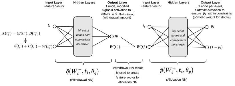
Figure 4.1: Illustration of the NN framework as per Section 4.2. Additional technical details can be found in Appendix D.

4.3 NN Estimate of the Optimal Control

Now we describe the training optimization problem for the proposed data driven NN framework, which is agnostic to the underlying data generation process. We assume that a set of asset return trajectories are available, which are used to approximate the expectation in (4.1) for any given control. For NN training, we approximate the expectation in (4.1) based on a finite number of samples as follows:

$$\hat{V}_{NN}(\bm{\theta}_{q},\bm{\theta}_{p},W^{*},s,b,t_{0}^{-})=\\ \tfrac{1}{N}\sum_{j=1}^{N}\Biggl{[}~{}\sum_{i=0}^{M}\hat{q}((W_{i})^{j},t_{i};\bm{\theta}_{q})~{}+~{}\kappa\biggl{(}W^{*}+\frac{1}{\alpha}\min((W_{T})^{j}-W^{*},0)\biggr{)}+\epsilon(W_{T})^{j}\bigg{|}X(t_{0}^{-})=(s,b)~{}\Biggr{]}~{}\\ \text{ subject to }\begin{cases}((S_{t})^{j},(B_{t})^{j})\text{ drawn from the $j^{th}$ sample of returns};~{}~{}t\notin\mathcal{T}\\ (W_{i}^{+})^{j}=(S_{i}^{-})^{j}+(B_{i}^{-})^{j}-\hat{q}\left((W_{t_{i}}^{-})^{j},t_{i},\bm{\theta_{q}}\right)\,;~{}(X_{i}^{+})^{j}=(S_{i}^{+},B_{i}^{+})^{j}\\ (S_{i}^{+})^{j}=\hat{p}\left((W_{i}^{+})^{j},t_{i},\bm{\theta_{p}}\right)~{}(W_{i}^{+})^{j}\,;~{}(B_{i}^{+})^{j}=(1-\hat{p}\left((W_{i}^{+})^{j},t_{i},\bm{\theta_{p}})\right)~{}(W_{i}^{+})^{j}\,\\ \left(\hat{q}_{i}(\cdot),\hat{p}_{i}(\cdot)\right)\in\mathcal{Z}\left((W_{i}^{-})^{j},(W_{i}^{+})^{j},t_{i}\right)\\ i=0,\ldots,M~{};~{}t_{i}\in\mathcal{T}\\ \end{cases}~{},$$ (4.4)

where the superscript $j$ represents the $j^{\text{th}}$ path of joint asset returns and $N$ is the total number of sampled paths. For subsequent benchmark comparison, we generate price paths using processes (2.3) and (2.4). We are, however, agnostic as to the method used to generate these paths. We assume that the random sample paths are independent, but that correlations can exist between returns of different assets. In addition, correlation between the returns of different time periods can also be represented, e.g., block bootstrap resampling is designed to capture autocorrelation in the time series data.

The optimal parameters obtained by training the neural network are used to generate the control functions $\hat{q}^{*}(\cdot):=\hat{q}(\cdot;\bm{\theta_{q}^{*}})$ and $\hat{p}^{*}(\cdot):=\hat{p}(\cdot;\bm{\theta_{p}^{*}})$, respectively. With these functions, we can evaluate the performance of the generated control on testing data sets that are out-of-sample or out-of-distribution. We present the detailed results of such tests in Section 7.

5 Data

For the computational study in this paper, we use data from the Center for Research in Security Prices (CRSP) on a monthly basis over the 1926:1-2019:12 period. The specific indices used are the CRSP 10-year U.S. Treasury index for the bond asset and the CRSP value-weighted total return index for the stock asset. All of these various indexes are in nominal terms, so we adjust them for inflation by using the U.S. CPI index, also supplied by CRSP. We use real indexes since investors funding retirement spending should be focused on real (not nominal) wealth goals.

We use the above market data in two different ways in subsequent investigations:

1. Stochastic model calibration: Any data set referred to in this paper as synthetic data is generated by parametric stochastic models (SDEs) (as described in Section 2.2), whose parameters are calibrated to the CRSP data by using the threshold technique (Mancini, 2009; Cont and Mancini, 2011; Dang and Forsyth, 2016). The data is inflation-adjusted so that all parameters reflect real returns. Table E.1 shows the results of calibrating the models to the historical data. The correlation $\rho_{sb}$ is computed by removing any returns which occur at times corresponding to jumps in either series. See Dang and Forsyth (2016) for details of the technique for detecting jumps.

2. Bootstrap resampling: Any data set referred to in this paper as historical data is generated by using the stationary block bootstrap method (Politis and Romano, 1994; Politis and White, 2004; Patton et al., 2009; Dichtl et al., 2016) to resample the historical CRSP data set. This method involves repeatedly drawing randomly sampled blocks of random size, with replacement, from the original data set. The block size follows a geometric distribution with a specified expected block size. To preserve correlation between asset returns, we use a paired sampling approach to simultaneously draw returns from both time series. This, in effect, shuffles the original data and can be repeated to obtain however many resampled paths one desires. Since the order of returns in the sequence is unchanged within the sampled block, this method accounts for some possible serial correlation in market data. Detailed pseudo-code for this method of block bootstrap resampling is given in Forsyth and Vetzal (2019).

   We note that block resampling is commonly used by practitioners and academics (see for example Anarkulova et al. (2022); Dichtl et al. (2016); Scott and Cavaglia (2017); Simonian and Martirosyan (2022); Cogneau and Zakamouline (2013)). Block bootstrap resampling will be used to carry out robustness checks in Section 7. Note that for any realistic number of samples and expected block size, the probability of repeating a resampled path is negligible (Ni et al., 2022).

   One important parameter for the block resampling method is the expected block size. Forsyth (2022) determines that a reasonable expected block size for paired resampling is about three months. The algorithm presented in Patton et al. (2009) is used to determine the optimal expected block size for the bond and stock returns separately; see Table F.1. Subsequently, we will also test the sensitivity of the results to a range of block sizes from 1 to 12 months in numerical experiments.

To train the neural networks, we require that the number of sampled paths, $N$, be sufficiently large to fully represent the underlying market dynamics. Subsequently, we first generate training data through Monte Carlo simulations of the parametric models described in (2.3) and (2.4). We emphasize however that in the proposed data driven NN framework, we only require return trajectories of the underlying assets. In later sections, we present results from NNs trained on non-parametrically generated data, e.g. resampled historical data. We also demonstrate the NN framework’s robustness on test data.

6 Computational Results

We now present and compare performance of the optimal control from the HJB PDE and NN method respectively on synthetic data, with investment specifications given in Table 6.1. Each strategy’s performance is measured w.r.t. to the objective function in (2.22), which is a weighted reward (EW) and risk (ES) measure. To trace out an efficient frontier in the (EW,ES) plane, we vary $\kappa$ (the curve represents the (EW,ES) performance on a set of optimal Pareto points).

We first present strategies computed from the HJB framework described in Section 3. We verify that the numerical solutions are sufficiently accurate, so that this solution can be regarded as ground truth. We then present results computed using the NN framework of Section 4, and demonstrate the accuracy of the NN results by comparing to the ground truth computed from the HJB equation. We carry out further analysis by selecting an interesting point on the (EW,ES) efficient frontier, in particular $\kappa=1.0$, to study in greater detail. The point $\kappa=1.0$ is at the knee of the efficient frontier, which makes it desirable in terms of risk-reward tradeoff (picking the exact $\kappa$ will be a matter of investor preference, however). This notion of the knee point is loosely based on the concept of a compromise solution of multi-objective optimization problems, which selects the point on the efficient frontier with the minimum distance to an unattainable ideal point (Marler and Arora, 2004). For this knee point of $\kappa=1.0$, we analyze the controls and wealth outcomes under both frameworks. We also discuss some key differences between the HJB and NN frameworks’ results and their implications.

Investment horizon $T$ (years)	30
Equity market index	CRSP Cap-weighted index (real)
Bond index	10-year Treasury (US) (real)
Initial portfolio value $W_{0}$	1000
Cash withdrawal times	$t=0,1,\ldots,30$
Withdrawal range	$[35,60]$
Equity fraction range	$[0,1]$
Borrowing spread $\mu_{c}^{b}$	0.0
Rebalancing interval (years)	1
Market parameters	See Appendix E

Table 6.1: Problem setup and input data. Monetary units: thousands of dollars.

6.1 Strategies Computed from HJB Equation

We carry out a convergence test for the HJB framework by tracing the efficient frontier (i.e. varying the scalarization parameter $\kappa$) for solutions of varying refinement levels (i.e. number of grid points in the $(s,b)$ directions). Figure 6.1 shows these efficient frontiers. As the efficient frontiers from various grid sizes all practically overlap each other, this demonstrates convergence of solutions computed from solving HJB equations. Table G.1 shows a convergence test for a single point on the frontier. The convergence is roughly first-order (for the value function). This convergence test justifies the use of the HJB framework results as a ground-truth.

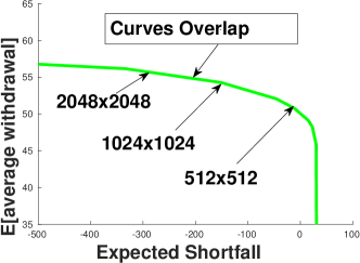
Figure 6.1: EW-ES frontier, computed from problem (2.22). Note: Scenario in Table 6.1. Comparison of HJB solution performance with varying grid sizes. HJB solution performance computed on $2.56\times 10^{6}$ observations of synthetic data. Parameters for synthetic data based on cap-weighted real CRSP, real 10 year treasuries (see Table E.1). $q_{min}=35,q_{\max}=60$. $\epsilon=10^{-6}$. Units: thousands of dollars.

Remark 6.1 (Effect of Stabilization Term $\epsilon W_{T}$).

Recall the stabilization term, $\epsilon W_{T}$, introduced in (2.22). We now provide motivation for its inclusion, and observe its effect on the control $\hat{\mathcal{P}}$. When $W_{t}\gg W^{*}$ and $t\to T$, the control will only weakly affect the objective function. This is because, in this situation, $Pr[W_{T}<W^{*}]\simeq 0$ and thus the allocation control will have little effect on the ES term in the objective (recall that $W^{*}$ is held constant for the induced time consistent strategy, see Appendix A). In addition, the withdrawal is capped at $q_{\max}$ for very high values of $W_{t}$, so the withdrawal control does not depend on $W_{t}$ in this case either. The stabilization term can be used to alleviate ill-posedness of the problem in this region.

In Figure 6.2, we present the heat map of the allocation control computed from the HJB framework. Subplot (a) presents allocation control heat map for a small positive stabilization parameter $\epsilon=10^{-6}$, while Subplot (b) presents allocation control heat map with $\epsilon=-10^{-6}$. In the ill-posed region (the top right region of the heat maps), the presence of $\epsilon W_{T}$, with $\epsilon=10^{-6}$, forces the control to invest 100% in stocks to generate high terminal wealth. Conversely, changing the stabilization parameter to be negative ($\epsilon=-10^{-6}$) forces the control to invest completely in bonds.

We observe that the control behaves differently only at high level of wealth as $t\to T$ in both cases. The 5th and the 50th percentiles of control on the synthetic data set behave similarly in both the positive and negative $\epsilon$ cases. The 95th percentile curve tends towards higher wealth during later phases of the investment period when the $\epsilon$ is positive (Figure 2(a)), whereas the curve tends downward when $\epsilon$ is negative (Figure 2(b)). When the magnitude of $\epsilon$ is sufficiently small, the inclusion of $\epsilon W_{T}$ in the objective function does not change summary statistics (to four decimal places when $|\epsilon|=10^{-6}$). While the choice of negative or positive $\epsilon$ with small magnitude can lead to different allocation control scenarios at high wealth level near the end of time horizon, the choice makes little difference from the perspective of the problem $PCEE_{t_{0}}(\kappa)$. If the investor reaches very high wealth near $T$, the choice between 100% stocks and 100% bonds does not matter as the investor always ends with $W_{T}\gg W^{*}$. Our experiments show that the control $q$ is unaffected when the magnitude of $\epsilon$ is small and continues to call for maximum withdrawals at high levels of wealth as $t\to T$, just as described in Remark 6.1.

Comparing the optimal withdrawal strategy determined by solving stochastic optimal control problem (2.22) with a fixed withdrawal strategy (both strategies with dynamic asset allocation), Forsyth (2022) finds that the stochastic optimal strategy (4.4) is much more efficient in withdrawing cash over the investment horizon. Accepting a very small amount of additional risk, the retiree can dramatically increase total withdrawals. For a more detailed discussion of the optimal control, we refer the reader to Forsyth (2022).

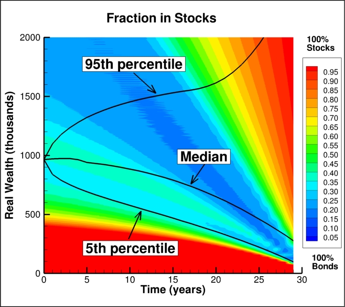
(a) Fraction in stocks, HJB Control, $\epsilon=10^{-6}$

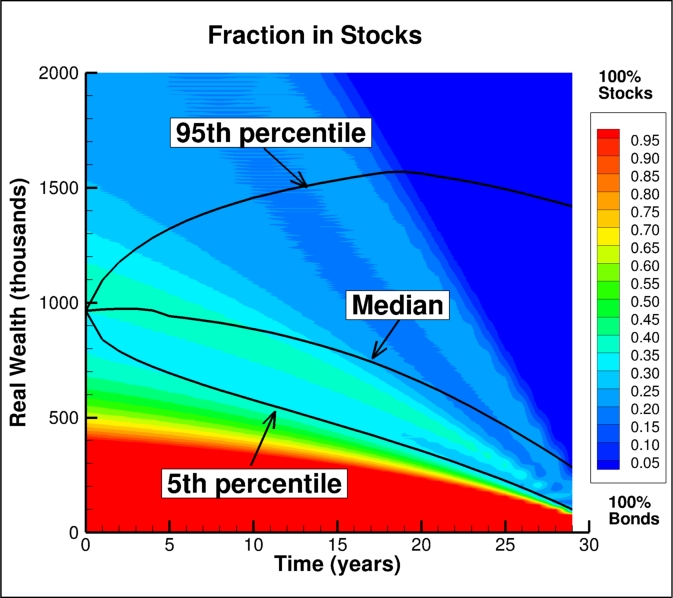
(b) Fraction in stocks, HJB Control, $\epsilon=-10^{-6}$

Figure 6.2: Effect of $\epsilon$: fraction in stocks computed from the problem (2.22). Note: investment setup is as in Table 6.1. HJB solution performance computed on $2.56\times 10^{6}$ observations of synthetic data. Parameters for synthetic data based on cap-weighted real CRSP, real 10 year treasuries (see Table E.1). $q_{min}=35,q_{\max}=60$, $\kappa=1.0$. $W^{*}=58.0$ for PIDE results. (a)$~{}\epsilon=10^{-6}$. (b)$~{}\epsilon=-10^{-6}$. Units: thousands of dollars.

6.2 Accuracy of Strategy Computed from NN framework

We compute the NN control following the framework discussed in Section 4. We compare the efficient frontiers obtained from the HJB equation solution and the NN solution. From Figure 6.3, the NN control efficient frontier is almost indistinguishable from the HJB control efficient frontier. Detailed summary statistics for each computed point on the frontier can be found in Appendix H.2, and a comparison of objective function values, for the NN and HJB control at each frontier point, can be found in Appendix H.3. For most points on the frontier, the difference in objective function values, from NN and HJB, is less than $0.1\%$. This demonstrates that the accuracy of the NN framework approximation of the ground-truth solution is more than adequate, considering that the difference between the NN solution and the PDE solution is about the same as the estimated PDE error (see Table G.1).

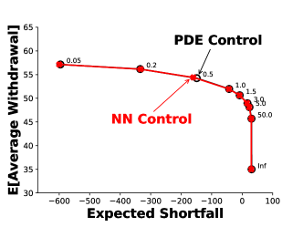
Figure 6.3: Comparison of EW-ES frontier for the Neural Network (NN) and Hamilton-Jacobi-Bellman (HJB) Partial Differential Equation (PDE) methods, computed from the problem (2.22). Note: investment setup in Table 6.1. HJB solution performance computed on $2.56\times 10^{6}$ observations of synthetic data. Parameters for synthetic data based on cap-weighted real CRSP, real 10 year treasuries (see Table E.1). Control computed from the NN model, trained on $2.56\times 10^{6}$ observations of synthetic data. $q_{min}=35,q_{\max}=60$. $\epsilon=10^{-6}$. Units: thousands of dollars. Labels on nodes indicate $\kappa$ parameter.

We now further analyze the control $\hat{\mathcal{P}}$ produced by the NN framework for $\kappa=1$. Comparing Figure 4(b) with Figure 4(d), we observe that the withdrawal control $\hat{q}$ produced by the NN is practically identical to the withdrawal control produced by the HJB framework. However, there are differences in the allocation control heat maps. The NN heat map for allocation control $p$ (Figure 4(a)) appears most similar to that of the HJB allocation heat map for negative $\epsilon$ (Figure 2(b)), but it is clear that the NN allocation heat map differs significantly from the HJB heat map for positive $\epsilon$ (Figure 2(a)) at high level of wealth as $t\to T$. The NN allocation control behaves differently from the HJB controls in this region, choosing a mix of stocks and bonds instead of choosing a 100% allocation in a single asset. Noting this difference is only at higher level of wealth near $T$, we see that the 5th percentile and the median wealth curves are indistinguishable. The NN control’s 95th percentile curve, however, is different and indeed the curve is in between the 95th percentile curves from the negative and positive versions of the HJB-generated control.

Drawing from this, we attribute the NN framework’s inability to fully replicate the HJB control to the ill-posedness of the optimal control problem in the (top-right) region of high wealth levels near $T$. The small value of $\epsilon$ means that the stabilization term contributes a very small fraction of the objective function value and thus has a very small gradient, relative to the first two terms in the objective function. Since we use stochastic gradient descent for optimization, we see a very small impact of $\epsilon$. Moreover, the data for high levels of wealth as $t\to T$ is very sparse and so the effect of the small gradient is further reduced. As a result, the NN appears to smoothly extrapolate in this region and therefore avoids investment into a single asset. Recall that in Section 6.1, we stated that the choice in the signs of $\epsilon$, with small $\epsilon$, in the stabilization term is somewhat arbitrary and does not affect summary statistics. Therefore, we see that the controls produced by the two methods only differ in irrelevant aspects, at least based on the EW and ES reward-risk consideration.

NN Control Results

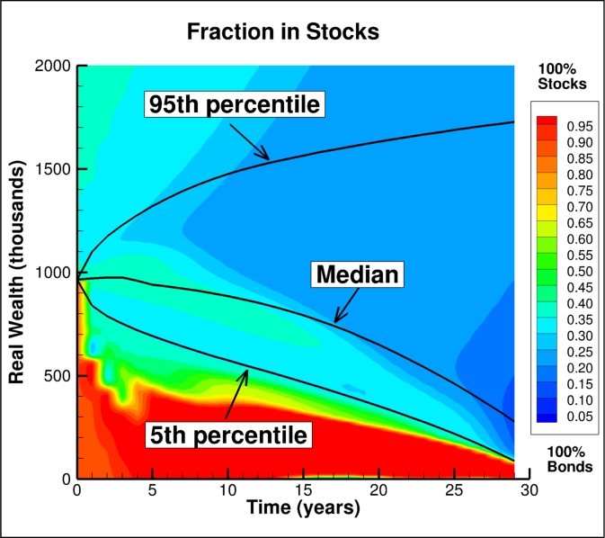
(a) Fraction in stocks, NN Control

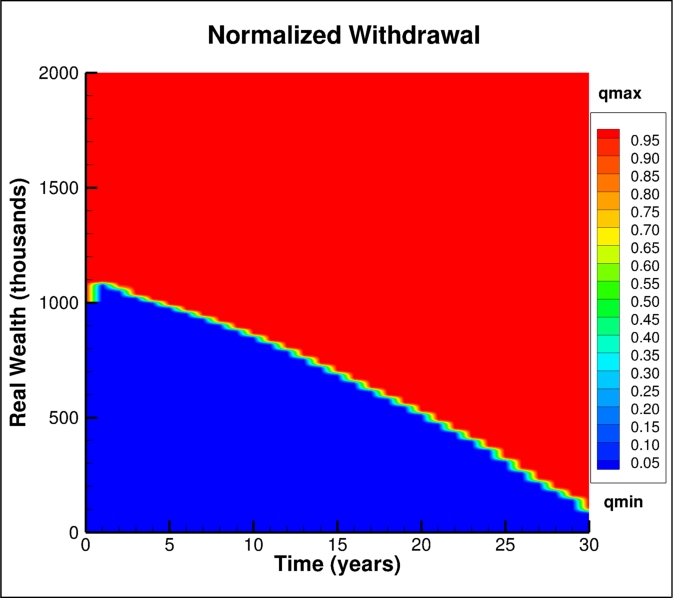
(b) Withdrawals, NN Control

HJB Control Results

(c) Fraction in stocks, HJB Control

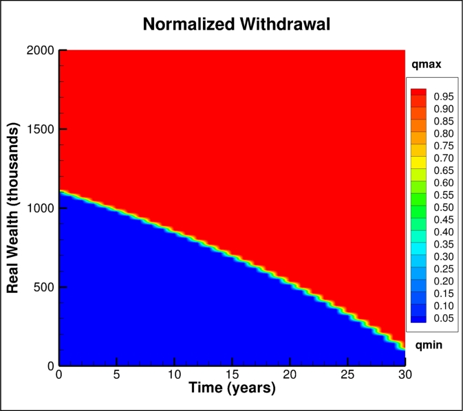
(d) Withdrawals, HJB Control

Figure 6.4: Heat map of controls: fraction in stocks and withdrawals, computed from the problem (2.22). Note: problem setup described in Table 6.1. HJB solution performance computed on $2.56\times 10^{6}$ observations of synthetic data. Parameters for synthetic data based on cap-weighted real CRSP, real 10 year treasuries (see Table E.1). NN model trained on $2.56\times 10^{6}$ observations of synthetic data. $q_{min}=35,q_{\max}=60$, $\kappa=1.0$. $W^{*}=59.1$ for NN results. $W^{*}=58.0$ for the HJB results. $\epsilon=10^{-6}$. Normalized withdrawal $(q-q_{\min})/(q_{\max}-q_{\min})$. Units: thousands of dollars.

NN Control Results

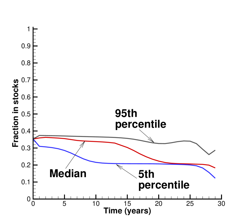
(a) Percentiles fraction in stocks, NN Control, $\epsilon=10^{-6}$

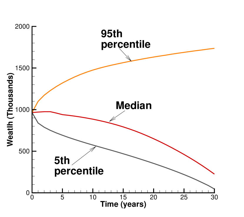
(b) Percentiles wealth, NN Control, $\epsilon=10^{-6}$

(c) Percentiles withdrawals, NN Control, $\epsilon=10^{-6}$

HJB Control Results (Positive and Negative Stabilization)

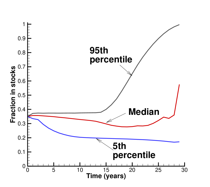
(d) Percentiles fraction in stocks, HJB Control, $\epsilon=10^{-6}$

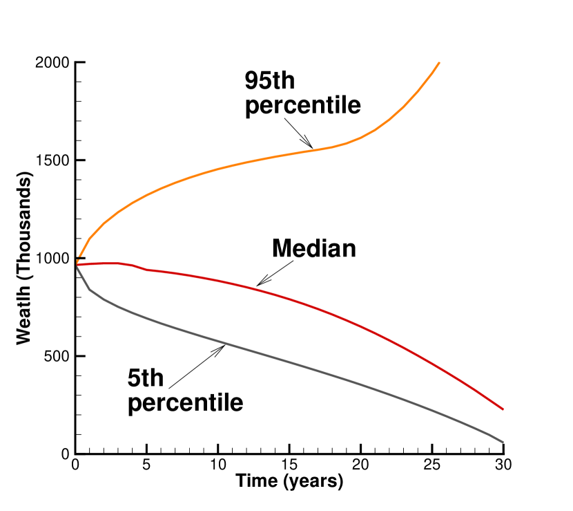
(e) Percentiles wealth, HJB Control, $\epsilon=10^{-6}$

(f) Percentiles withdrawals, HJB Control, $\epsilon=10^{-6}$

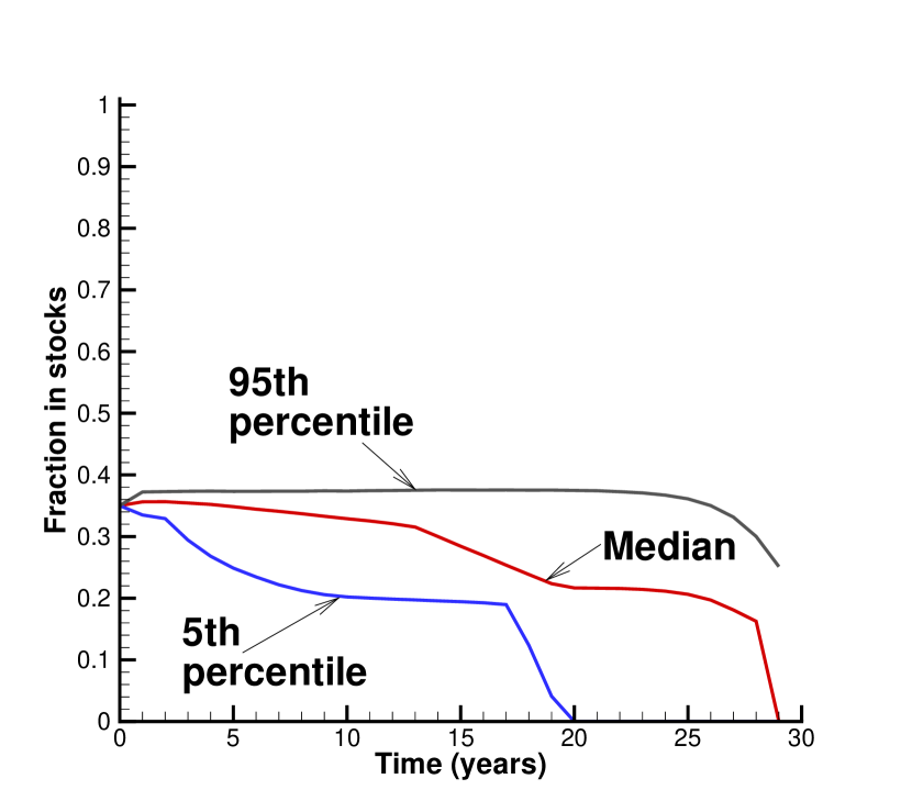
(g) Percentiles fraction in stocks, HJB Control, $\epsilon=-10^{-6}$

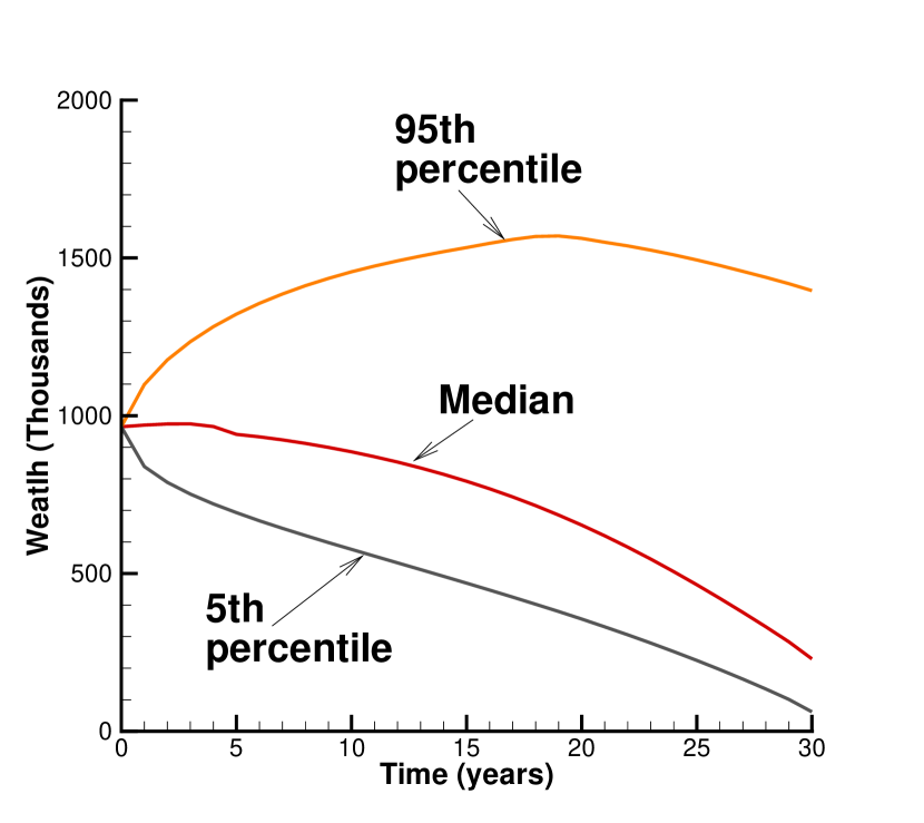
(h) Percentiles wealth, HJB Control, $\epsilon=-10^{-6}$

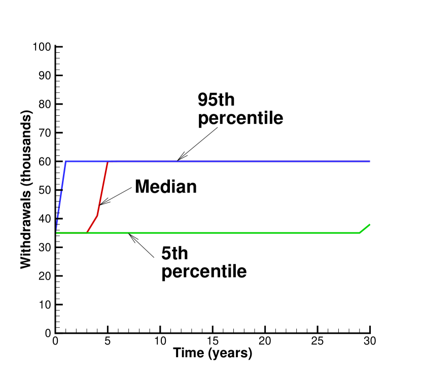
(i) Percentiles withdrawals, HJB Control, $\epsilon=-10^{-6}$

Figure 6.5: Scenario in Table 6.1. NN and HJB controls computed from the problem (2.22). Parameters based on the real CRSP index, and real 10-year treasuries (see Table E.1). NN model trained on $2.56\times 10^{5}$ observations of synthetic data. HJB framework results from $2.56\times 10^{6}$ observations of synthetic data. $q_{min}=35,q_{\max}=60$, $\kappa=1.0$. $W^{*}=59.1$ for NN results. $W^{*}=58.0$ for HJB results. Units: thousands of dollars.

It is interesting to observe that the proposed neural network framework is able to produce the bang-bang withdrawal control computed in Forsyth (2022), especially since we are using the continuous function $\hat{q}$ as an approximation. A bang-bang control switches abruptly as shown here: the optimal strategy is to withdraw the minimum if the wealth is below a threshold, or else withdraw the maximum. As expected, the control threshold decreases as we move forward in time. We can see that the NN and HJB withdrawal controls behave very similarly at the 95th, 50th, and 5th percentiles of wealth (Figures 5(c) and 5(f)). Essentially, the optimal strategy withdraws at either $q_{\max}$ or $q_{\min}$, with a very small transition zone. This is in line with our expectations. By withdrawing less and investing more initially, the individual decreases the chance of running out of savings.

We also note that the NN allocation control presents a small spread between the 5th and 95th percentile of the fraction in stocks (Figure 5(a)). In fact, the maximum stock allocation for the 95th percentile never exceeds 40%, indicating that this is a stable low-risk strategy, which as we shall see, outperforms the Bengen (1994) strategy.

7 Model Robustness

A common pitfall of neural networks is over-fitting to the training data. Neural networks that are over-fitted do not have the ability to generalize to previously unseen data. Since future asset return paths cannot be predicted, it is important to ascertain that the computed strategy is not overfitted to the training data and can perform well on unseen return paths. In this section, we demonstrate the robustness of the NN model’s generated controls.

We conduct three types of robustness tests: (i) out-of-sample testing, (ii) out-of-distribution testing, and (iii) control sensitivity to training distribution.

7.1 Out-of-sample testing

Out-of-sample tests involve testing model performance on an unseen data set sampled from the same distribution. In our case, this means training the NN on one set of SDE paths sampled from the parametric model, and testing on another set of paths generated using a different random seed. We present the efficient frontier generated by computed controls on this new data set in Figure 7.1, which shows almost unchanged performance on the out-of-sample test set.

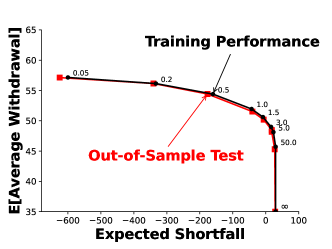
Figure 7.1: Out-of-sample test. EW-ES frontiers, computed from the problem (2.22). Note: Scenario in Table 6.1. Comparison of NN training performance results vs. out-of-sample test. Both training and testing data are $2.56\times 10^{5}$ observations of synthetic data, generated with a different random seed. Parameters for synthetic data based on cap-weighted real CRSP, real 10 year treasuries (see Table E.1). $q_{min}=35,q_{\max}=60$. $\epsilon=10^{-6}$. Units: thousands of dollars. Labels on nodes indicate $\kappa$ parameter values.

7.2 Out-of-distribution testing

Out-of-distribution testing involves evaluating the performance of the computed control on an entirely new data set sampled from a different distribution. Specifically, test data is not generated from the parametric model used to produce training data, but is instead bootstrap resampled from historical market returns via the method described in Section 5. We vary the expected block sizes to generate multiple testing data sets of $2.56\times 10^{5}$ paths.

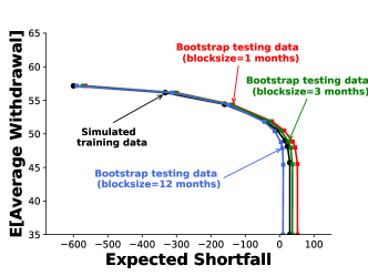
Figure 7.2: Out-of-distribution test. EW-ES frontiers of controls generated by NN model trained on $2.56\times 10^{5}$ observations of synthetic data, tested on $2.56\times 10^{5}$ observations of historical data with varying expected block sizes. Computed from the problem (2.22). Note: Setup as in Table 6.1. Parameters based on real CRSP index and real 10-year U.S. Treasuries (see Table E.1). Historical data in range 1926:1-2019:12. Units: thousands of dollars. $q_{min}=35;q_{max}=60$. Simulated training data refers to Monte Carlo simulations using the SDEs (2.3) and (2.4).

In Figure 7.2, we see that for each block size tested, the efficient frontiers are fairly close, indicating that the controls are relatively robust. Note that the efficient frontiers for test performance in the historical market with expected block size of 1 and 3 months plot slightly above the synthetic market frontier. We conjecture that this may be due to more pessimistic tail events in the synthetic market.

The out-of-sample and out-of-distribution tests verify that the neural network is not over-fitting to the training data, and is generating an effective strategy, at least based on our block resampling data.

7.3 Control sensitivity to training distribution

To test the NN framework’s adaptability to other training data sets, we train the NN framework on historical data (with expected block sizes of both 3 months and 12 months) and then test the resulting control on synthetic data. In Figure 7.3, we compare the training performance and the test performance. The EW-ES frontiers for the test results on the synthetic data are very close to the results on the bootstrap market data (training data set). This shows the NN framework’s adaptability to use alternative data sets to learn, with the added advantage of not being reliant on a parametric model, which is prone to miscalibration. Figure  7.3 also shows that, in all cases, in the synthetic or historical market, the EW-ES control significantly outperforms the Bengen 4% Rule (Bengen, 1994).

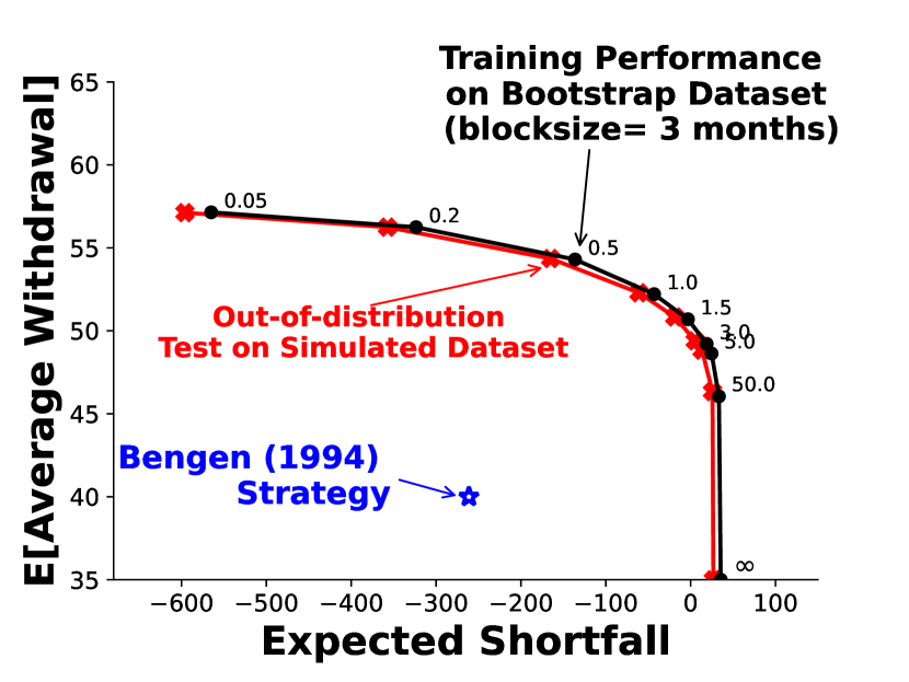
(a) Historical training data, block size = 3 months

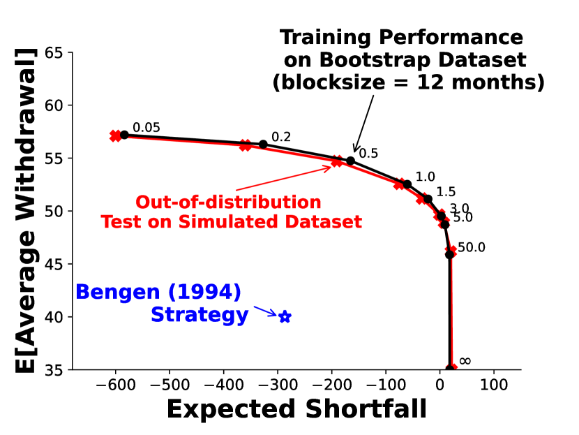
(b) Historical training data, block size = 12 months

Figure 7.3: Training on historical data. EW-ES frontiers of controls generated by NN model trained on $2.56\times 10^{5}$ observations of historical data with expected block sizes of a) 3 months and b) 12 months, each tested on $2.56\times 10^{5}$ observations of synthetic data. Parameters based on real CRSP index and real 10-year U.S. Treasuries (see Table E.1). Historical data in range 1926:1-2019:12. Units: thousands of dollars. $q_{min}=35;q_{max}=60$. The Bengen (1994) results are based on bootstrap resampling of the historical data. Labels on nodes indicate $\kappa$ parameter values. Simulated testing data refers to Monte Carlo simulations using the SDEs (2.3) and (2.4). $\epsilon=+10^{-6}$.

8 Conclusion

In this paper, we proposed a novel neural network (NN) architecture to efficiently and accurately compute the optimal decumulation strategy for retirees with DC pension plans. The stochastically constrained optimal control problem is solved based on a single standard unconstrained optimization, without using dynamic programming.

We began by highlighting the increasing prevalence of DC pension plans over traditional DB pension plans, and outlining the critical decumulation problem that faces DC plan investors. There is an extensive literature on devising strategies for this problem. In particular, we examine a Hamilton-Jacobi-Bellman (HJB) Partial Differential Equation (PDE) based approach that can be shown to converge to an optimal solution for a dynamic withdrawal/allocation strategy. This provides an attractive balance of risk management and withdrawal efficiency for retirees. In this paper, we seek to build upon this approach by developing a new, more versatile framework using NNs to solve the decumulation problem.

We conduct computational investigations to demonstrate the accuracy and robustness of the proposed NN solution, utilizing the unique opportunity to compare NN solutions with the HJB results as a ground truth. Of particular noteworthiness is that the continuous function approximation from the NN framework is able to approximate a bang-bang control with high accuracy. We extend our experiments to establish the robustness of our approach, testing the NN control’s performance on both synthetic and historical data sets.

We demonstrate that the proposed NN framework produced solution accurately approximates the ground truth solution. We also note the following advantages of the proposed NN framework:

1. The NN method is data driven, and does not require postulating and calibrating a parametric model for market processes.

2. The NN method directly estimates the low dimensional control by solving a single unconstrained optimization problem, avoiding the problems associated with dynamic programming methods, which require estimating high dimensional conditional expectations (see van Staden et al. (2023)).

3. The NN formulation maintains its simple structure (discussed in Section 4.2), immediately extendable to problems with more frequent rebalancing and/or withdrawal events. In fact, the problem presented in (2.22) requires each control NN to have only two hidden layers for 30 rebalancing and withdrawal periods.

4. The approximated control maintains continuity in time and/or space, provided it exists, or otherwise provides a smooth approximation. Continuity of the allocation control $p$ is an important practical consideration for any investment policy.

Due to the ill-posedness of the stochastic optimal control problem in the region of high wealth near the end of the decumulation horizon, we observe that the NN allocation can appear to be very different from the HJB PDE solution. We note, however, that both strategies yield indistinguishable performance when assessed with the expected withdrawal and ES reward-risk criteria. In other words, these differences hardly affect the objective function value, a weighted reward and risk value. In the region of high wealth level near the end of the time horizon, the retiree is free to choose whether to invest 100% in stocks or 100% in bonds, since this has a negligible effect on the objective function value (or reward-risk consideration).

To conclude, the advantages of the NN framework make it a more versatile method, compared to the solution of the HJB PDE. We expect that the NN approach can handle problems of higher complexity, e.g., involving a higher number of assets. In addition, the NN method can be applied to other proposed formulations for the retirement planning problem (for example, see Forsyth et al. (2022)). We leave the extension of this methodology to future work.

9 Acknowledgements

Forsyth’s work was supported by the Natural Sciences and Engineering Research Council of Canada (NSERC) grant RGPIN-2017-03760. Li’s work was supported by the Natural Sciences and Engineering Research Council of Canada (NSERC) grant RGPIN-2020-04331. The author’s are grateful to P. van Staden for supplying the initial software library for NN control problems.

10 Conflicts of interest

The authors have no conflicts of interest to report.

Appendix

Appendix A Induced Time Consistent Policy

In this section of the appendix, we review the concept of time consistency and relate its relevance to the $PCEE_{t_{0}}(\kappa)$ problem, (2.22).

Consider the optimal control $\mathcal{P}^{*}$ for problem (2.22),

$$(\mathcal{P}^{*})^{t_{0}}(X(t_{i}^{-}),t_{i})~{};~{}i=0,\ldots,M~{}.$$ (A.1)

Equation (A.1) can be interpreted as the optimal control for any time $t_{i}\geq t_{0}$, as a function of the state variables $X(t)$, as computed at $t_{0}$.

Now consider if we were to solve the problem (2.22) starting at a later time $t_{k},k>0$. This optimal control starting at $t_{k}$ is denoted by:

$$(\mathcal{P}^{*})^{t_{k}}(X(t_{i}^{-}),t_{i})~{};~{}i=k,\ldots,M\}~{}.$$ (A.2)

In general, the solution of (2.22) computed at $t_{k}$ is not equivalent to the solution computed $t_{0}$:

$$(\mathcal{P}^{*})^{t_{k}}(X(t_{i}^{-}),t_{i})\neq(\mathcal{P}^{*})^{t_{0}}(X(t_{i}^{-}),t_{i})~{};~{}i\geq k>0.$$ (A.3)

This non-equivalence makes problem (2.22) time inconsistent, implying that the investor will have the incentive to deviate from the control computed at time $t_{0}$ at later times. This type of control is considered a pre-commitment control since the investor would need to commit to following the strategy at all times following $t_{0}$. Some authors describe pre-commitment controls as non-implementable because of the incentive to deviate.

In our case, however, the pre-commitment control from (2.22) can be shown to be identical to the time consistent control for an alternative version of the objective function. By holding $W^{*}$ fixed at the optimal value (at time zero), we can define the time consistent equivalent problem (TCEQ). Noting that the inner supremum in (2.22) is a continuous function of $W^{*}$, we define the optimal value of $W^{*}$ as

$$\mathcal{W}^{*}(s,b) = \displaystyle\mathop{\rm arg\,max}_{W^{*}}\biggl{\{}\sup_{\mathcal{P}_{0}\in\mathcal{A}}\Biggl{\{}E_{\mathcal{P}_{0}}^{X_{0}^{-},t_{0}^{-}}\Biggl{[}~{}\sum_{i=0}^{M}q_{i}~{}+~{}\kappa\biggl{(}W^{*}+\frac{1}{\alpha}\min(W_{T}-W^{*},0)\biggr{)}\bigg{|}X(t_{0}^{-})=(s,b)~{}\Biggr{]}\Biggr{\}}~{}.$$

With a given initial wealth of $W_{0}^{-}$, this gives the following result from Forsyth (2020):

Proposition A.1 (Pre-commitment strategy equivalence to a time consistent policy for an alternative objective function).

The pre-commitment EW-ES strategy found by solving $J\left(s,b,t_{0}^{-}\right)$ from (2.22), with fixed $W^{*}=\mathcal{W}^{*}$ from Equation LABEL:pcee_argmax, is identical to the time consistent strategy for the equivalent problem TCEQ (which has fixed $\mathcal{W}^{*}(0,W_{0}^{-})$), with the following value function:

$$\left(\mathit{TCEQ_{t_{n}}}\left(\kappa/\alpha\right)\right):$$

$$\tilde{J}\left(s,b,t_{n}^{-}\right) = \sup_{\mathcal{P}_{n}\in\mathcal{A}}\Biggl{\{}E_{\mathcal{P}_{n}}^{X_{n}^{-},t_{n}^{-}}\Biggl{[}~{}\sum_{i=n}^{M}q_{i}~{}+~{}\frac{\kappa}{\alpha}\min(W_{T}-\mathcal{W}^{*}(0,W_{0}^{-}),0)\Biggr{.}\Biggr{.}\bigg{|}X(t_{n}^{-})=(s,b)~{}\Biggr{]}\Biggr{\}}.$$

Proof.

This follows similar steps as in Forsyth (2020), proof of Proposition (6.2). ∎

With fixed $W^{*}$, $\mathit{TCEQ_{t_{n}}}(\kappa/\alpha)$ is based on a target-based shortfall as its measure of risk, which is trivially time consistent. $W^{*}$ has the convenient interpretation of a disaster level of final wealth, as specified at time zero. Since the optimal controls for $PCEE_{t_{0}}(\kappa)$ and $\mathit{TCEQ_{t_{n}}}(\kappa/\alpha)$ are identical, we regard $\mathit{TCEQ_{t_{n}}}(\kappa/\alpha)$ as the EW-ES induced time consistent strategy (Strub et al., 2019), which is implementable since the investor will have no incentive to deviate from a strategy computed at $t_{0}$ at later times.

For further discussion concerning the relationship between pre-commitment, time consistent, and induced time consistent strategies, we refer the reader to Bjork and Murgoci (2010; 2014); Vigna (2014; 2022); Strub et al. (2019); Forsyth (2020); Bjork et al. (2021).

Appendix B PIDE Between Rebalancing Times

Applying Ito’s Lemma for jump processes (Tankov and Cont, 2009), using Equations (2.3) and (2.4) in Equation (LABEL:expanded_6) gives

$$V_{t}+\frac{(\sigma^{s})^{2}s^{2}}{2}V_{ss}+(\mu^{s}-\lambda_{\xi}^{s}\gamma_{\xi}^{s})sV_{s}+\lambda_{\xi}^{s}\int_{-\infty}^{+\infty}V(e^{y}s,b,t)f^{s}(y)~{}dy+\frac{(\sigma^{b})^{2}b^{2}}{2}V_{bb}$$

$$~{}~{}~{}+(\mu^{b}+\mu_{c}^{b}{\bf{1}}_{\{b<0\}}-\lambda_{\xi}^{b}\gamma_{\xi}^{b})bV_{b}+\lambda_{\xi}^{b}\int_{-\infty}^{+\infty}V(s,e^{y}b,t)f^{b}(y)~{}dy-(\lambda_{\xi}^{s}+\lambda_{\xi}^{b})V+\rho_{sb}\sigma^{s}\sigma^{b}sbV_{sb}=0~{},$$

$$~{}~{}~{}~{}~{}~{}~{}~{}~{}~{}~{}~{}~{}~{}~{}~{}~{}~{}~{}~{}~{}~{}~{}~{}~{}~{}~{}~{}~{}~{}~{}s\geq 0~{}.$$ (B.1)

where the density functions $f^{s}(y),f^{b}(y)$ are as given in equation (2.1).

Appendix C Computational Details: Hamilton-Jacobi-Bellman (HJB) PDE Framework

For a detailed description of the numerical algorithm used to solve the HJB equation framework described in Section 3, we refer the reader to Forsyth (2022). We summarize the method here.

First, we solve the auxiliary problem (3.2), with fixed values of $W^{*}$, $\kappa$ and $\alpha$. The state space in $s>0$ and $b>0$ is discretized using evenly spaced nodes in log space to create a grid to represent cases. A separate grid is created in a similar fashion to represent cases where wealth is negative. The Fourier methods discussed in Forsyth and Labahn (2019) are used to solve the PIDE representing market dynamics between rebalancing times. Both controls for withdrawal and allocation are discretized using equally spaced grids. The optimization problem (3.6) is solved first for the allocation control by exhaustive search, storing the optimal for each discretized wealth node. The withdrawal control in (LABEL:q_opt) can then be solved in a similar fashion, using the previously stored allocation control to evaluate the right-hand side of (LABEL:q_opt). Linear interpolation is used where necessary. The stored controls are used to advance the solution in (3.9).

Since the numerical method just described assumes a constant $W^{*}$, an outer optimization step to find the optimal $W^{*}$ (candidate Value-at-Risk) is necessary. Given an approximate solution to (3.2) at $t=0$, the full solution to $PCEE_{t_{0}}(\kappa)$ (2.22) is determined using Equation (3.11). A coarse grid is used at first for an exhaustive search. This is then used as the starting point for a one-dimensional optimization algorithm on finer grids.

Appendix D Computational Details: NN Framework

D.1 NN Optimization

The NN framework, as described in Section 4 and illustrated in Figure 4.1, was implemented using the PyTorch library (Paszke et al., 2019). The withdrawal network $\hat{q}$, and allocation network $\hat{p}$ were both implemented with 2 hidden layers of 10 nodes each, with biases. Stochastic Gradient Descent (Ruder, 2016) was used in conjunction with the Adaptive Momentum optimization algorithm to train the NN framework (Kingma and Ba, 2014). The NN parameters and auxiliary training parameter $W^{*}$ were trained with different initial learning rates. The same decay parameters and learning rate schedule were used. Weight decay ($\ell_{2}$ penalty) was also employed to make training more stable. The training loop utilizes the auto-differentiation capabilities of the PyTorch library. Hyper-parameters used for NN training in this paper’s experiments are given in Table D.1.

The training loop tracks the minimum loss function value as training progresses and selects the model that had given the optimal loss function value based on the entire training dataset by the end of the specified number of training epochs.

D.2 Transfer learning between different $\kappa$ points

For high values of $\kappa$, the objective function is weighted more towards optimizing ES (lower risk). In these cases, optimal controls are more difficult to compute. This is because the ES measure used (CVAR) is only affected by the sample paths below the $5^{th}$ percentile of terminal wealth, which are quite sparse. To overcome these training difficulties, we employ transfer learning (Tan et al., 2018) to improve training for the more difficult points on the efficient frontier. We begin training the model for the lowest $\kappa$ from a random initialization (‘cold-start’), and then initialize the models for each increasing $\kappa$ with the model for the previous $\kappa$. Through numerical experiments, we found this method made training far more stable and less likely to terminate in local minima for higher values of $\kappa$.

D.3 Running minimum tracking

The training loop tracks the minimum loss function value as training progresses and selects the model that had given the optimal loss function value based on the entire training dataset by the end of the specified number of training epochs.

NN framework hyper-parameter	Value
Hidden layers per network	2
# of nodes per hidden layer	10
Nodes have biases	True
# of iterations (#itn)	50,000
SGD mini-batch size	1,000
# of training paths	$2.56\times 10^{5}$
Optimizer	Adaptive Momentum
Initial Adam learning rate for $(\bm{\theta}_{q},\bm{\theta}_{p})$	0.05
Initial Adam learning rate for $W^{*}$	0.04
Adam learning rate decay schedule	$[0.70\times\text{\#itn},0.97\times\text{\#itn}]$, $\gamma=0.20$
Adam $\beta_{1}$	0.9
Adam $\beta_{2}$	0.998
Adam weight decay ($\ell_{2}$ Penalty)	0.0001
Transfer Learning between $\kappa$ points	True
Take running minimum as result	True

Table D.1: Hyper-parameters used in training the NN framework for numerical experiments presented in this paper.

D.4 Standardization

To improve learning for the neural network, we normalize the input wealth using means and standard deviations of wealth samples from a reference strategy. We use the constant withdrawal and allocation strategy defined in Forsyth (2022) as the reference strategy with $2.56\times 10^{5}$ simulated paths. Let $W^{b}_{t}$ denote the wealth vector at time $t$ based on simulations. Then $\bar{W}^{b}_{t}$ and $\sigma(W^{b}_{t})$ denote the associated average wealth and standard deviation. Then we normalize the feature input to the neural network in the following way:

$$\tilde{W_{t}}=\frac{W_{t}-\bar{W}^{b}_{t}}{\sigma(W^{b}_{t})}$$

For the purpose of training the neural network, the values $\bar{W}^{b}_{t}$ and $\sigma(W^{b}_{t})$ are just constants, and we can use any reasonable values. This input feature normalization is done for both withdrawal and allocation NNs.

In Section 7, we show in out-of-sample and out-of-distribution tests that $\bar{W}^{b}_{t}$ and $\sigma(W^{b}_{t})$ do not need to be related to the testing data as long as these are reasonable values. In Section 4, when referring to $W$ as part of the input to the NN functions $\hat{q}$ and $\hat{p}$, we use the standardized $\tilde{W}$ for computation.

Appendix E Model Calibrated from Market Data

Table E.1 shows the calibrated model parameters for processes (2.3) and (2.4), from Forsyth (2022) using market data described in §5.

Calibrated Model Parameters

CRSP	$\mu^{s}$	$\sigma^{s}$	$\lambda^{s}$	$u^{s}$	$\eta_{1}^{s}$	$\eta_{2}^{s}$	$\rho_{sb}$
	0.0877	0.1459	0.3191	0.2333	4.3608	5.504	0.04554
10-year Treasury	$\mu^{b}$	$\sigma^{b}$	$\lambda^{b}$	$u^{b}$	$\eta_{1}^{b}$	$\eta_{2}^{b}$	$\rho_{sb}$
	0.0239	0.0538	0.3830	0.6111	16.19	17.27	0.04554

Table E.1: Estimated annualized parameters for double exponential jump diffusion model. Value-weighted CRSP index, 10-year US treasury index deflated by the CPI. Sample period 1926:1 to 2019:12.

Appendix F Optimal expected block sizes: bootstrap resampling

Table F.1 shows our estimates of the optimal block size using the algorithm in Politis and White (2004); Patton et al. (2009) using market data described in §5.

Optimal expected block size for bootstrap resampling historical data

Data series	Optimal expected
	block size $\hat{b}$ (months)
Real 10-year Treasury index	4.2
Real CRSP value-weighted index	3.1

Table F.1: Optimal expected blocksize $\hat{b}=1/v$ when the blocksize follows a geometric distribution $Pr(b=k)=(1-v)^{k-1}v$. The algorithm in Patton et al. (2009) is used to determine $\hat{b}$. Historical data range 1926:1-2019:12.

Appendix G Convergence Test: HJB Equation

Table G.1 shows a detailed convergence test for a single point on the (EW, ES) frontier, using the PIDE method. The controls are computed using the HJB PDE, and stored. The stored controls are then used in Monte Carlo simulations, which are used to verify the PDE solution, and also generate various statistics of interest.

Algorithm in Section 3					Monte Carlo
Grid	ES (5%)	$E[\sum_{i}q_{i}]/(M+1)$	Value Function	$W^{*}$	ES (5%)	$E[\sum_{i}q_{i}]/(M+1)$
$512\times 512$	-51.302	52.056	1.562430e+3	50.10	-45.936	52.07
$1024\times 1024$	-46.239	52.049	1.567299e+3	52.47	-45.102	52.05
$2048\times 2048$	-42.594	51.976	1.568671e+3	58.00	-42.623	51.97
$4096\times 4096$	-40.879	51.932	1.569025e+3	61.08	-41.250	51.93

Table G.1: HJB equation convergence test, real stock index: deflated real capitalization weighted CRSP, real bond index: deflated ten year treasuries. Scenario in Table 6.1. Parameters in Table E.1. The Monte Carlo method used $2.56\times 10^{6}$ simulations. $\kappa=1.0,\alpha=.05$. Grid refers to the grid used in the Algorithm in Section 3: $n_{x}\times n_{b}$, where $n_{x}$ is the number of nodes in the $\log s$ direction, and $n_{b}$ is the number of nodes in the $\log b$ direction. Units: thousands of dollars (real). $(M+1)$ is the total number of withdrawals. $M$ is the number of rebalancing dates. $q_{\min}=35.0$. $q_{\max}=60$. Algorithm in Section 3.

Appendix H Detailed efficient frontier comparisons

Table H.1 shows the detailed efficient frontier, computed using the HJB equation method, using the $2048\times 2048$ grid. Table H.2 shows the efficient frontier computed from the NN framework. This should be compared to Table H.1. Table H.3 compares the objective function values, at various points on the efficient frontier, for the HJB and NN frameworks.

Detailed Efficient Frontier: HJB Framework

$\kappa$	ES (5%)	$E[\sum_{i}q_{i}]/(M+1)$	$Median[W_{T}]$
0.05	-596.00	57.14	124.36
0.2	-334.29	56.17	92.99
0.5	-148.99	54.25	111.20
1.0	-42.62	51.97	227.84
1.5	-8.05	50.63	298.20
3.0	17.42	48.95	380.36
5.0	24.09	48.12	414.60
50.0	30.60	45.70	519.03
$\infty$	31.00	35.00	1003.47

Table H.1: Synthetic market results for HJB framework optimal strategies. Gives the detailed results used to construct HJB efficient frontier in Figure 6.3. Assumes the scenario given in Table 6.1. Stock index: real capitalization weighted CRSP stocks; bond index: ten year treasuries. Parameters from Table E.1. Units: thousands of dollars. Statistics based on $2.56\times 10^{6}$ Monte Carlo simulation runs. Control is computed using the Algorithm in Section 3, ($2048\times 2048$ grid) stored, and then used in the Monte Carlo simulations. $q_{\min}=35.0$, $q_{\max}=60$. $(M+1)$ is the number of withdrawals. $M$ is the number of rebalancing dates. $\epsilon=10^{-6}$.

Detailed Efficient Frontier: NN Framework
$\kappa$ ES (5%) $E[\sum_{i}q_{i}]/(M+1)$ $\text{\emph{Median}}[W_{T}]$ 0.05 -599.81 57.15 106.23 0.2 -333.01 56.14 78.59 0.5 -160.14 54.40 105.05 1 -43.02 51.95 227.79 1.5 -8.57 50.62 302.17 3 16.01 48.99 374.43 5 23.20 48.13 425.13 50 29.88 45.72 493.41 $\infty$ 29.90 35.00 947.60

Table H.2: Synthetic market results for NN framework optimal strategies. Gives the detailed results used to construct NN efficient frontier in Figure 6.3. Assumes the scenario given in Table 6.1. Stock index: real capitalization weighted CRSP stocks; bond index: ten year treasuries. Parameters from Table E.1. Units: thousands of dollars. Training performance statistics based on $2.56\times 10^{5}$ Monte Carlo simulation runs. Control is computed using the algorithm in Section 4. $q_{\min}=35.0$, $q_{\max}=60$. $(M+1)$ is the number of withdrawals. $M$ is the number of rebalancing dates. $\epsilon=10^{-6}$.

Objective Function Value Comparison: HJB Framework vs. NN Framework
$\kappa$ HJB equation NN % difference 0.05 1741.54 1741.71 0.01% 0.2 1674.41 1673.81 -0.04% 0.5 1607.26 1606.44 -0.05% 1 1568.45 1567.34 -0.07% 1.5 1557.46 1556.22 -0.08% 3 1569.71 1566.86 -0.18% 5 1612.16 1607.86 -0.27% 50 2946.70 2911.10 -1.21%

Table H.3: Objective function value comparison for the HJB equation and NN framework model results on range of $\kappa$ values. Objective function values for both frameworks computed according to $PCEE_{t0}(\kappa)$ (higher is better). Assuming the scenario given in Table 6.1. Stock index: real capitalization weighted CRSP stocks; bond index: ten year treasuries. Parameters from Table E.1. HJB solution statistics based on $2.56\times 10^{6}$ Monte Carlo simulation runs. HJB control is computed using the Algorithm in Section 3, ($2048\times 2048$ grid) stored, and then used in the Monte Carlo simulations. NN Training performance statistics based on $2.56\times 10^{5}$ Monte Carlo simulation runs. Control is computed using the NN framework in Section 4. $q_{\min}=35.0$, $q_{\max}=60$. $(M+1)$ is the number of withdrawals. $M$ is the number of rebalancing dates. $\epsilon=10^{-6}$.

References

- Anarkulova et al. (2022) Anarkulova, A., S. Cederburg, and M. S. O’Doherty (2022). Stocks for the long run? evidence from a broad sample of developed markets. Journal of Financial Economics 143(1), 409–433.
- Bengen (1994) Bengen, W. (1994). Determining withdrawal rates using historical data. Journal of Financial Planning 7, 171–180.
- Bernhardt and Donnelly (2018) Bernhardt, T. and C. Donnelly (2018). Pension decumulation strategies: A state of the art report. Technical Report, Risk Insight Lab, Heriot Watt University.
- Bjork et al. (2021) Bjork, T., M. Khapko, and A. Murgoci (2021). Time inconsistent control theory with finance applications. Springer Finance, New York.
- Bjork and Murgoci (2010) Bjork, T. and A. Murgoci (2010). A general theory of Markovian time inconsistent stochastic control problems. SSRN 1694759.
- Bjork and Murgoci (2014) Bjork, T. and A. Murgoci (2014). A theory of Markovian time inconsisent stochastic control in discrete time. Finance and Stochastics 18, 545–592.
- Boukherouaa et al. (2021) Boukherouaa, E. B., K. AlAjmi, J. Deodoro, A. Farias, and R. Ravikumar (2021). Powering the digital economy: Opportunities and risks of artificial intelligence in finance. IMF Departmental Papers 2021(024), A001.
- Buehler et al. (2019) Buehler, H., L. Gonon, J. Teichmann, and B. Wood (2019). Deep hedging. Quantitative Finance 19(8), 1271–1291.
- Cogneau and Zakamouline (2013) Cogneau, P. and V. Zakamouline (2013). Block bootstrap methods and the choice of stocks for the long run. Quantitative Finance 13:9, 1443–1457.
- Cont and Mancini (2011) Cont, R. and C. Mancini (2011). Nonparametric tests for pathwise properties of semimartingales. Bernoulli 17, 781–813.
- Dang and Forsyth (2014) Dang, D.-M. and P. A. Forsyth (2014). Continuous time mean-variance optimal portfolio allocation under jump diffusion: a numerical impulse control approach. Numerical Methods for Partial Differential Equations 30, 664–698.
- Dang and Forsyth (2016) Dang, D.-M. and P. A. Forsyth (2016). Better than pre-commitment mean-variance portfolio allocation strategies: a semi-self-financing Hamilton-Jacobi-Bellman equation approach. European Journal of Operational Research 250, 827–841.
- Dichtl et al. (2016) Dichtl, H., W. Drobetz, and M. Wambach (2016). Testing rebalancing strategies for stock-bond portfolios across different asset allocations. Applied Economics 48(9), 772–788.
- Forsyth and Labahn (2019) Forsyth, P. and G. Labahn (2019). Monotone Fourier methods for optimal stochastic control in finance. Journal of Computational Finance 22:4, 25–71.
- Forsyth (2020) Forsyth, P. A. (2020). Multi-period mean CVAR asset allocation: Is it advantageous to be time consistent? SIAM Journal on Financial Mathematics 11:2, 358–384.
- Forsyth (2022) Forsyth, P. A. (2022). A stochastic control approach to defined contribution plan decumulation: The nastiest, hardest problem in finance. North American Actuarial Journal 26:2, 227–251.
- Forsyth and Vetzal (2019) Forsyth, P. A. and K. R. Vetzal (2019). Optimal asset allocation for retirement savings: deterministic vs. time consistent adaptive strategies. Applied Mathematical Finance 26:1, 1–37.
- Forsyth et al. (2022) Forsyth, P. A., K. R. Vetzal, and G. Westmacott (2022). Optimal performance of a tontine overlay subject to withdrawal constraints. arXiv 2211.10509 .
- Han and E (2016) Han, J. and W. E (2016). Deep learning approximation for stochastic control problems. CoRR abs/1611.07422.
- Homer and Sylla (2005) Homer, S. and R. Sylla (2005). A History of Interest Rates. Wiley, New York.
- Huré et al. (2021) Huré, C., H. Pham, A. Bachouch, and N. Langrené (2021). Deep neural networks algorithms for stochastic control problems on finite horizon: Convergence analysis. SIAM Journal on Numerical Analysis 59:1, 525–557.
- Ismailov (2022) Ismailov, V. (2022). A three layer neural network can represent any multivariate function ArXiv:2012.03016.
- Kingma and Ba (2014) Kingma, D. and J. Ba (2014). Adam: A method for stochastic optimization p. arXiv:1412.6980.
- Kou (2002) Kou, S. G. (2002). A jump-diffusion model for option pricing. Management Science 48, 1086–1101.
- Kou and Wang (2004) Kou, S. G. and H. Wang (2004). Option pricing under a double exponential jump diffusion model. Management Science 50, 1178–1192.
- Laurière et al. (2021) Laurière, M., O. Pironneau, et al. (2021). Performance of a markovian neural network versus dynamic programming on a fishing control problem. arXiv preprint arXiv:2109.06856 .
- Lin et al. (2015) Lin, Y., R. MacMinn, and R. Tian (2015). De-risking defined benefit plans. Insurance: Mathematics and Economics 63, 52–65.
- MacDonald et al. (2013) MacDonald, B.-J., B. Jones, R. J. Morrison, R. L. Brown, and M. Hardy (2013). Research and reality: A literature review on drawing down retirement financial savings. North American Actuarial Journal 17, 181–215.
- MacMinn et al. (2014) MacMinn, R., P. Brockett, J. Wang, Y. Lin, and R. Tian (2014). The securitization of longevity risk and its implications for retirement security. In O. S. Mitchell, R. Maurer, and P. B. Hammond, eds., Recreating Sustainable Retirement, pp. 134–160. Oxford University Press, Oxford.
- Mancini (2009) Mancini, C. (2009). Non-parametric threshold estimation models with stochastic diffusion coefficient and jumps. Scandinavian Journal of Statistics 36, 270–296.
- Marler and Arora (2004) Marler, R. and J. Arora (2004). Survey of multi-objective optimization methods for engineering. Structural and Multidisciplinary Optimization 26, 369–395.
- Ni et al. (2022) Ni, C., Y. Li, P. Forsyth, and R. Carroll (2022). Optimal asset allocation for outperforming a stochastic benchmark target. Quantitative Finance 22:9, 1595–1626.
- Paszke et al. (2019) Paszke, A., S. Gross, F. Massa, A. Lerer, J. Bradbury, G. Chanan, T. Killeen, Z. Lin, N. Gimelshein, L. Antiga, A. Desmaison, A. Kopf, E. Yang, Z. DeVito, M. Raison, A. Tejani, S. Chilamkurthy, B. Steiner, L. Fang, J. Bai, and S. Chintala (2019). Pytorch: An imperative style, high-performance deep learning library. In Advances in Neural Information Processing Systems 32, pp. 8024–8035. Curran Associates, Inc.
- Patton et al. (2009) Patton, A., D. Politis, and H. White (2009). Correction to: automatic block-length selection for the dependent bootstrap. Econometric Reviews 28, 372–375.
- Pfau (2018) Pfau, W. D. (2018). An overview of retirement income planning. Journal of Financial Counseling and Planning 29:1, 114:120.
- Pfeiffer et al. (2013) Pfeiffer, S., J. R. Salter, and H. E. Evensky (2013). Increasing the sustainable withdrawal rate using the standby reverse mortgage. Journal of Financial Planning 26:12, 55–62.
- Politis and Romano (1994) Politis, D. and J. Romano (1994). The stationary bootstrap. Journal of the American Statistical Association 89, 1303–1313.
- Politis and White (2004) Politis, D. and H. White (2004). Automatic block-length selection for the dependent bootstrap. Econometric Reviews 23, 53–70.
- Powell (2021) Powell, W. B. (2021). From reinforcement learning to optimal control: A unified framework for s equential decisions. In K. G. Vamvoudakis, Y. Wan, F. L. Lewis, and D. Cansever, eds., Handbook of Reinforcement Learning and Control, pp. 29–74. Springer International Publishing.
- Ritholz (2017) Ritholz, B. (2017). Tackling the ‘nastiest, hardest problem in finance’. www.bloomberg.com/view/articles/2017-06-05/tackling-the-nastiest-hardest-problem-in-finance.
- Rockafellar and Uryasev (2000) Rockafellar, R. T. and S. Uryasev (2000). Optimization of conditional value-at-risk. Journal of Risk 2, 21–42.
- Ruder (2016) Ruder, S. (2016). An overview of gradient descent optimization algorithms. arXiv:1609.04747 .
- Scott et al. (2009) Scott, J., W. Sharpe, and J. Watson (2009). The 4% rule – at what price? Journal of Investment Management 7:3, 31–48.
- Scott and Cavaglia (2017) Scott, L. and S. Cavaglia (2017). A wealth management perspective on factor premia and the value of downside protection. Journal of Portfolio Management 43(3), 33–41.
- Shefrin and Thaler (1988) Shefrin, H. M. and R. H. Thaler (1988). The behavioral life-cycle hypothesis. Economic Inquiry 26:4, 609–643.
- Simonian and Martirosyan (2022) Simonian, J. and A. Martirosyan (2022). Sharpe parity redux. The Journal of Portfolio Management 48:4, 183–193.
- Strub et al. (2019) Strub, M., D. Li, and X. Cui (2019). An enhanced mean-variance framework for robo-advising applications. SSRN 3302111.
- Tan et al. (2018) Tan, C., F. Sun, T. Kong, W. Zhang, C. Yang, and C. Liu (2018). A survey on deep transfer learning. arXiv 1808.01974 .
- Tankov and Cont (2009) Tankov, P. and R. Cont (2009). Financial Modelling with Jump Processes. Chapman and Hall/CRC, New York.
- Tsang and Wong (2020) Tsang, K. H. and H. Y. Wong (2020). Deep-learning solution to portfolio selection with serially-dependent returns. SIAM Journal on Financial Mathematics 11:2, 593–619.
- U.S. Bureau of Labor Statistics (2022) U.S. Bureau of Labor Statistics (2022). Employee benefits survey: Latest numbers. https://www.bls.gov/ebs/latest-numbers.htm.
- van Staden et al. (2023) van Staden, P., P. Forsyth, and Y. Li (2023). Beating a benchmark: dynamic programming may not be the right numerical approach. SIAM Journal on Financial Mathematics 14:2, 407–451.
- Vigna (2014) Vigna, E. (2014). On efficiency of mean-variance based portfolio selection in defined contribution pension schemes. Quantitative Finance 14, 237–258.
- Vigna (2022) Vigna, E. (2022). Tail optimality and preferences consistency for intertemporal optimization problems. SIAM Journal on Financial Mathematics 13:1, 295–320.
- Williams and Kawashima (2023) Williams, R. and C. Kawashima (2023). Beyond the 4% rule: How much can you spend in retirement? https://www.schwab.com/learn/story/beyond-4-rule-how-much-can-you-spend-retirement.