Magnetic scattering with spin-momentum locking: Single scatterers and diffraction grating

Abstract

Simultaneous manipulation of charge and spin density distributions in materials is the key element required in spintronics applications. Here we study the formation of coupled spin and charge densities arising in scattering of electrons by domains of local magnetization producing a position-dependent Zeeman field in the presence of the spin-momentum locking typical for topological insulators. Analytically and numerically calculated scattering pattern is determined by the electron energy, domain magnetization, and size. The spin-momentum locking produces strong differences with respect to the spin-diagonal scattering and leads to the scattering asymmetry with nonzero mean scattering angle as determined by only two parameters characterizing the system. To extend the variety of possible patterns, we study scattering by diffraction gratings and propose to design them in modern nanostructures based on topological insulators to produce desired distributions of the charge and spin densities. These results can be useful for engineering of magnetic patterns for electron optics to control coupled charge and spin evolution.

I Introduction: electron optics with spin-momentum locking

The ability to manipulate and control electron charge and spin dynamics by external fields is one of the challenges in modern applied physics. This goal can be achieved by electron optics, that is using elements similar to conventional optics based on wave properties of electrons. Another option is related to the electron spin optics, that is to control both coupled electron spins and charge dynamics. A conventional tool to manipulate electron spin is the Zeeman-like coupling either with the external magnetic field or with material magnetization. However, simultaneous control of spin and charge motion requires spin-orbit coupling Bychkov1984 resulting in spin-momentum locking. This can be achieved by using electrons in low-energy two-dimensional surface states of topological insulators, where this coupling demonstrates itself as a strong spin-momentum locking expressed in the Hamiltonian Hasan2010 ; Qi2011

$$H=-i\hbar v\mbox{\boldmath$\sigma$}\cdot{\bm{\nabla}+}\Delta_{\rm m}(\mathbf{r})\sigma_{z},$$ (1)

and produces relativistic-like Dirac cones. Here position $\mathbf{r}=(x,y),$ $v$ is the electron bandstructure velocity parameter and $\Delta_{\rm m}(\mathbf{r})$ is the local magnetization assumed to be along the $z-$axis. We assume that the electron energy is considerably low and the corresponding momentum is sufficiently small to satisfy the validity of the Hamiltonian (1), including only the linear $\mbox{\boldmath$\sigma$}\cdot{\bm{\nabla}}$ term and neglecting the band warping Fu2009 , with $\sigma_{i}$ being the Pauli matrices. Here it is convenient to present the electron spin in the form ${\bm{\sigma}}=({\bm{\sigma}}_{\perp},\sigma_{z}),$ where ${\bm{\sigma}}_{\perp}=(\sigma_{x},\sigma_{y})$ is the two-dimensional in-plane component. The velocity of the electron defined as $\mathbf{v}=i[H,\mathbf{r}]/\hbar=v(\sigma_{x},\sigma_{y})=v{\bm{\sigma}}_{\perp}$ is determined by the electron spin. Thus, by acting at the electron spin by a position- and time-dependent Zeeman field one can modify the electron velocity and, thus, influence the charge transport (see, e.g., Ref. [Yokoyama2011, ] for electron propagation in the presence of one-dimensional stripe-like magnetization). Recently, Ref. [Mochida2022, ] analyzed the effects of skew scattering by magnetic monopoles in spin-orbit coupled systems.

On the one hand, random magnetic disorder modifies weak localization Hikami1980 in conventional semiconductors and strongly influences the conductivity of topological insulators Kudla2019 . On the other hand, the ability to produce magnetization pattern $\Delta_{\rm m}(\mathbf{r})$ Katmis2016 ; Tokura2019 permits design of position-dependent spin dynamics and, correspondingly, the manipulation of electron wavefunction producing the coupled spin-charge transport Jamali2015 ; Chiba2017 ; Chen2020 . The effects of spin-dependent velocity are known for conventional semiconductors for electrons Rokhinson2004 and holes Rendell2022 and can manifest itself in electron scattering by impurities in the presence of strong spin-orbit coupling Hutchinson2017 , formation of equilibrium spin currents Rashba2004 ; Tokatly2010 and in the spin-Hall effect Dyakonov1971 ; Sinova2004 ; Murakami2003 ; Kato2004 ; Mishchenko2004 ; Sih2005 ; Wunderlich2005 kinetics.

Here we explore the possibility to control electron spin and position dynamics by a single- and arrays of magnetized quantum dots with spatially confined magnetization on the surface of topological insulators. One possible application is the variety of spin torques Mellnik2014 ; Ndiaye2017 ; Han2017 ; Ghosh2017 ; Mahendra2018 ; Moghaddam2020 ; Han2021 ; Bondarenko2017 produced on the magnetized quantum dots by scattered electrons to manage magnetization dynamics and coupled spin-charge transport. We study the scattering processes in different regimes and conclude that a net charge current injection can be produced. Based on the results of a single-dot scattering approach, we propose to design diffraction gratings made by a one-dimensional array of magnetic quantum dots for this purpose. This grating will produce on purpose asymmetric patterns of spin and charge densities and currents.

The rest of the paper is organized as follows. In Sec. II we formulate the scattering problem and present the observables of interest. In Sec. III we describe partial wave summation approach and present general analytical results. Different sets of parameters and scattering domains for single scatterers will be analyzed in Sec. IV while scattering by diffraction grating will be considered in Sec. V. The main numerical results for cross-section and scattering angles will be presented in Sec. VI. Section VII provides the conclusions and outlook of this paper.

II Scattering process and observables

For a circular magnetized disk on the surface of topological insulator we rewrite Eq. (1) in the form:

$$H=-iv\mbox{\boldmath$\sigma$}\cdot{\bm{\nabla}}+\theta(R-r)\Delta_{\rm m}\sigma_{z},$$ (2)

where $\theta(R-r)\Delta_{\rm m}$ is the local magnetization with the Heaviside function $\theta(R-r),$ as shown in Fig. 1. Here and below we use the system of units with $\hbar\equiv\,1.$

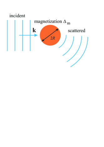
Figure 1: Asymmetric scattering of electron with the wavevector $\mathbf{k}$ by a single magnetized nanodot.

In the absence of external magnetization $(\Delta_{\rm m}\equiv 0)$ the free-space plane-wave function for ${\bm{\psi}}_{\mathbf{k}}(\mathbf{r})\sim e^{i\mathbf{k}\cdot\mathbf{r}}[\psi^{\uparrow}_{\mathbf{k}},\psi^{\downarrow}_{\mathbf{k}}]^{\mathrm{T}}$ (T stands for transposition) satisfies the equation:

$$\left[\begin{array}[]{cc}-\varepsilon&vk_{-}\\ vk_{+}&-\varepsilon\end{array}\right]\left[\begin{array}[]{c}\psi^{\uparrow}_{\mathbf{k}}\\ \psi^{\downarrow}_{\mathbf{k}}\end{array}\right]=0,$$ (3)

where $k_{\pm}\equiv\,k_{x}\pm ik_{y}$. We obtain two linear branches of spectrum $\varepsilon=\pm vk$ where $k=\sqrt{\,k_{x}^{2}+k_{y}^{2}}$ . For the eigenstates one has

$${\bm{\psi}}_{\mathbf{k}}(\mathbf{r})=\frac{e^{i\mathbf{k}\cdot\mathbf{r}}}{\sqrt{2}}\left[\begin{array}[]{c}1\\ \varepsilon\,k_{+}/|\varepsilon|\,k\end{array}\right].$$ (4)

and the spin is parallel $\left(\varepsilon>0\right)$ or antiparallel $\left(\varepsilon<0\right)$ to the momentum. At a large distance from the quantum dot the electron wavefunction at $\varepsilon>0$ is presented for the wave coming from $x=-\infty$ along the $x-$axis with $\mathbf{k}=(k,0)$ [Newton2013, ]

$${\bm{\psi}}(r,\varphi)=\frac{e^{ikx}}{\sqrt{2}}\left[\begin{array}[]{c}1\\ 1\end{array}\right]+{\bm{f}}(\varphi)\,\frac{e^{ikr}}{\sqrt{r}},$$ (5)

where

$${\bm{f}}(\varphi)=\left[\begin{array}[]{c}f^{\uparrow}(\varphi)\\ f^{\downarrow}(\varphi)\end{array}\right]$$ (6)

is the two-component spinor scattering amplitude. We note that in two-dimensional systems the cross-section $l$ has the length units and present the differential cross-section as $dl/d\varphi=|{\bm{f}}(\varphi)|^{2}$ where the total $l$ is:

$$l=\int_{-\pi}^{\pi}|{\bm{f}}(\varphi)|^{2}d\varphi.$$ (7)

Since, as we will demonstrate below, the scattering is anisotropic with $|{\bm{f}}(-\varphi)|\neq|{\bm{f}}(\varphi)|,$ we introduce the mean value of the scattering angle $\langle\varphi\rangle$ and of its square $\left\langle\varphi^{2}\right\rangle:$

$$\langle\varphi^{n}\rangle=\frac{1}{l}\int_{-\pi}^{\pi}\varphi^{n}|{\bm{f}}(\varphi)|^{2}d\varphi,$$ (8)

where $n=1$ or $n=2.$ The dispersion $D_{\varphi}=\sqrt{\langle\varphi^{2}\rangle-\langle\varphi\rangle^{2}}$, characterizes the width of the scattering aperture.

In addition, we mention that the asymmetric scattering produces effective charge current along the $y-$axis, which can be defined as:

$$\langle j\rangle=\frac{ev}{l}\int_{-\pi}^{\pi}\sin\varphi|{\bm{f}}(\varphi)|^{2}d\varphi$$ (9)

where $e$ is the electron charge. The behavior of this current as a function of system parameters is qualitatively similar to the behavior of $\left\langle\varphi\right\rangle.$

III Partial wave summation: analytical results

III.1 Wave functions and boundary conditions

In polar coordinates with $r=\sqrt{x^{2}+y^{2}}$, $\varphi=\arctan(y/x)$, the eigenstates in the form of the circular waves are determined by:

$$\left[\begin{array}[]{cc}\varepsilon-\Delta_{\rm m}(r)&ve^{-i\varphi}\left(i\,\partial_{r}+\displaystyle{\frac{\partial_{\varphi}}{r}}\right)\\ ve^{i\varphi}\left(i\,\partial_{r}-\displaystyle{\frac{\partial_{\varphi}}{r}}\right)&\varepsilon+\Delta_{\rm m}(r)\end{array}\right]{\bm{\psi}}(r,\varphi)=0.$$ (10)

To calculate the sum of partial waves attributed to the $z-$components of the angular momentum $m,$ we first substitute in Eq. (10) the spinor characterized by given $m$ in the form:

$${\bm{\psi}}_{m}(r,\varphi)=\,e^{im\varphi}\left[\begin{array}[]{c}\psi^{\uparrow}_{m}(r)\\ \psi^{\downarrow}_{m}(r)\,e^{i\varphi}\end{array}\right]$$ (11)

and obtain coupled equations for the radial functions (omitting the explicit $r-$dependence for brevity):

$$\left[\begin{array}[]{cc}\Delta_{\rm m}(r)-\varepsilon&-iv\left(\displaystyle{\frac{d}{dr}+\frac{m+1}{r}}\right)\\ -iv\left(\displaystyle{\frac{d}{dr}-\frac{m}{r}}\right)&-\Delta_{\rm m}(r)-\varepsilon\end{array}\right]\left[\begin{array}[]{c}\psi^{\uparrow}_{m}\\ \\ \\ \psi^{\downarrow}_{m}\end{array}\right]=0.$$ (12)

Inside the dot, $r<R$ and $\Delta_{\rm m}(r)=\Delta_{\rm m}:$

$$(\Delta_{\rm m}\,-\varepsilon)\,\psi^{\uparrow}_{m}-iv\left({\frac{d}{dr}+\frac{m+1}{r}}\right)\psi^{\downarrow}_{m}=0$$ (13)

$$-iv\left({\frac{d}{dr}-\frac{m}{r}}\right)\psi^{\uparrow}_{m}-(\Delta_{\rm m}\,+\varepsilon)\,\psi^{\downarrow}_{m}=0.$$ (14)

Extracting $\psi^{\downarrow}_{m}$ in Eq. (14)

$$\psi^{\downarrow}_{m}=-\frac{iv}{\Delta_{\rm m}\,+\varepsilon}\left({\frac{d}{dr}-\frac{m}{r}}\right)\psi^{\uparrow}_{m}$$ (15)

and substituting it into (13) we obtain for $\psi^{\uparrow}_{m}$

$$\kappa^{2}\psi^{\uparrow}_{m}-\left(\frac{d^{2}}{dr^{2}}+\frac{1}{r}\frac{d}{dr}-\frac{m^{2}}{r^{2}}\right)\psi^{\uparrow}_{m}=0,$$ (16)

with the energy-dependent $\kappa\equiv\sqrt{|\Delta_{\rm m}^{2}-\varepsilon^{2}|}/v.$ We begin with the realization $\varepsilon<\Delta_{\rm m}$ where the solution regular at $r\rightarrow 0$ is the modified Bessel function $\psi^{\uparrow}_{m}(r\kappa)=I_{m}(r\kappa)$ [Lebedev, ] and then consider the $\varepsilon>\Delta_{\rm m}$ case by analytical continuation. Using (15) we can write:

$$\psi^{\downarrow}_{m}(z)=-is\left(\frac{d}{dz}-\frac{m}{z}\right)\psi^{\uparrow}_{m}(z)=-isI_{m+1}(z),$$ (17)

where $z\equiv r\kappa$ and $s\equiv\sqrt{|\Delta_{\rm m}-\varepsilon|/(\Delta_{\rm m}+\varepsilon)}.$

Thus, the general solution at $r<R$ is

$$\left[\begin{array}[]{c}\psi^{\uparrow}_{m}\\ \psi^{\downarrow}_{m}\end{array}\right]=A_{m}\left[\begin{array}[]{c}I_{m}(\kappa r)\\ -isI_{m+1}(\kappa r)\end{array}\right],$$ (18)

where $A_{m}$ is a constant.

For $r>R$ with $\Delta_{\rm m}=0$ introducing for brevity $\mu\equiv\,r\varepsilon/v=kr$ we obtain

$$\left[\mu^{2}\frac{d^{2}}{d\mu^{2}}+\mu\frac{d}{d\mu}+(\mu^{2}-m^{2})\right]\psi^{\uparrow}_{m}=0,$$ (19)

with the Bessel functions $J_{m}(kr)$ and $Y_{m}(kr)$ [Lebedev, ] solutions where $\psi^{\downarrow}_{m}$ being expressed with $J_{m+1}(kr)$ and $Y_{m+1}(kr).$ The resulting general solution at $r>R$ is the superposition of the waves with harmonics

$$\left[\begin{array}[]{c}\psi^{\uparrow}_{m}\\ \psi^{\downarrow}_{m}\end{array}\right]=B_{m}\left[\begin{array}[]{c}J_{m}(kr)\\ iJ_{m+1}(kr)\end{array}\right]+C_{m}\left[\begin{array}[]{c}Y_{m}(kr)\\ iY_{m+1}(kr)\end{array}\right].$$ (20)

These equations are supplemented by the two continuity conditions at $r=R$ which can be reduced to a single equation as:

$$B_{m}J_{m}(kR)+C_{m}Y_{m}(kR)$$

$$= -\frac{I_{m}(\kappa R)}{sI_{m+1}(\kappa R)}\left(B_{m}J_{m+1}(kR)+C_{m}Y_{m+1}(kR)\right).$$

III.2 Scattering amplitude: summed partial waves

To perform summation over harmonics $m,$ we begin with the plane wave resolution $e^{ikr\cos\varphi}=\sum_{m=-\infty}^{\infty}i^{m}e^{im\varphi}\,J_{m}(kr)$smythe resulting in

$${\bm{\psi}}_{\mathbf{k}}(r,\varphi)=\frac{1}{\sqrt{2}}\left[\begin{array}[]{c}1\\ 1\end{array}\right]\sum_{m=-\infty}^{\infty}i^{m}e^{im\varphi}\,J_{m}(kr).$$ (22)

At large distances, $kr\gg|m^{2}-1/4|$, we use asymptotics of the Bessel functions Lebedev :

$${J}_{m}\left(kr\right) \simeq \sqrt{\frac{2}{\pi kr}}\cos\left(kr-\frac{m\pi}{2}-\frac{\pi}{4}\right),$$ (23)

$$Y_{m}\left(kr\right) \simeq \sqrt{\frac{2}{\pi kr}}\sin\left(kr-\frac{m\pi}{2}-\frac{\pi}{4}\right).$$ (24)

By using condition that the wave function contains only the outgoing $\exp(ikr)$ and no ingoing $\exp(-ikr)$ waves Newton2013 , that is the ingoing wave terms mutually cancel each other, we obtain

$$f^{\uparrow}(\varphi) = -ie^{-i\pi/4}\sqrt{\frac{1}{\pi k}}\sum_{-\infty}^{\infty}\frac{\gamma_{m}}{1+i\gamma_{m}}e^{im\varphi},$$ (25)

$$f^{\downarrow}(\varphi) = f^{\uparrow}\left(\varphi\right)e^{i\varphi}.$$ (26)

Here $\gamma_{m}\equiv\,C_{m}/B_{m}$ is obtained with the boundary conditions in the form of Eq. (III.1). The spin component expectation values for the scattered wave defined as

$$\sigma_{i}(\varphi)=\left\langle{\bm{f}}(\varphi)|\sigma_{i}|{\bm{f}}(\varphi)\right\rangle$$ (27)

are the same as those of the free state since $k_{+}=ke^{i\varphi}$ with $\sigma_{z}(\varphi)=0.$

In the low-energy domain $\varepsilon<\Delta_{\rm m}$ we obtain

$$\gamma_{m}=-\frac{sJ_{m}(kR)I_{m+1}(\kappa R)+I_{m}(\kappa R)J_{m+1}(kR)}{sY_{m}(kR)I_{m+1}(\kappa R)+I_{m}(\kappa R)Y_{m+1}(kR)}.$$ (28)

Similar calculation for the high-energy domain $\varepsilon>\Delta_{\rm m}$ using relation $I_{m}(i|z|)=\left(-i\right)^{m}J_{m}\left(-|z|\right)$ and $J_{m}(-x)=(-1)^{m}J_{m}(x)$ yields

$$\gamma_{m}=-\frac{sJ_{m}(kR)J_{m+1}(\kappa R)-J_{m}(\kappa R)J_{m+1}(kR)}{sY_{m}(kR)J_{m+1}(\kappa R)-J_{m}(\kappa R)Y_{m+1}(kR)}.$$ (29)

Various scattering regimes described by these equations will be discussed below analytically and numerically.

III.3 Scattering cross-section and asymmetry

It is convenient to introduce even $\Gamma_{g}\left(m_{1},m_{2}\right)=\Gamma_{g}\left(m_{2},m_{1}\right)$ and odd $\Gamma_{u}\left(m_{1},m_{2}\right)=-\Gamma_{u}\left(m_{2},m_{1}\right)$ matrices as

$$\frac{\gamma_{m_{1}}}{1-i\gamma_{m_{1}}}\frac{\gamma_{m_{2}}}{1+i\gamma_{m_{2}}}=\Gamma_{g}\left(m_{1},m_{2}\right)+\Gamma_{u}\left(m_{1},m_{2}\right)$$ (30)

$$\Gamma_{g}\left(m_{1},m_{2}\right)=\frac{\gamma_{m_{1}}\gamma_{m_{2}}}{\left(1+\gamma_{m_{1}}^{2}\right)\left(1+\gamma_{m_{2}}^{2}\right)}\left(1+\gamma_{m_{1}}\gamma_{m_{2}}\right)$$

$$\Gamma_{u}\left(m_{1},m_{2}\right)=i\frac{\gamma_{m_{1}}\gamma_{m_{2}}}{\left(1+\gamma_{m_{1}}^{2}\right)\left(1+\gamma_{m_{2}}^{2}\right)}\left(\gamma_{m_{1}}-\gamma_{m_{2}}\right),$$

and use them to define $l/R$, $\left\langle\varphi\right\rangle$ and $\left\langle\varphi^{2}\right\rangle.$ Using Eqs. (8), (25), (26), and (30), the $l/R$ and the mean value $\langle\varphi\rangle$ can be expressed with these matrices as:

$$\frac{l}{R} = \frac{4}{kR}\sum_{m}\frac{\gamma_{m}^{2}}{1+\gamma_{m}^{2}}=\frac{4}{kR}{\rm tr}\,\Gamma_{g}\left(m_{1},m_{2}\right),$$ (31)

$$\langle\varphi\rangle = -\frac{4i}{kl}\sum_{m_{1},m_{2}}\Gamma_{u}\left(m_{1},m_{2}\right)\frac{\left(-1\right)^{m_{2}-m_{1}}}{m_{2}-m_{1}}$$ (32)

making the scattering asymmetric with nonzero $\langle\varphi\rangle$ solely due to the imaginary terms $i\gamma_{m}$ in the denominators of Eqs. (25), (26), which appear due to the phase shift between the spin components in Eq. (11). This effect is qualitatively different from the spin-diagonal scattering by a radially-symmetric potential, which is always $\varphi\leftrightarrow\,-\varphi$ symmetric, and is similar to the scattering mechanisms producing the anomalous Hall effect Nagaosa2010 . For the $\langle\varphi^{2}\rangle$ we obtain similarly:

$$\langle\varphi^{2}\rangle=\frac{8}{kl}\sum_{m_{1},m_{2}}\Gamma_{g}\left(m_{1},m_{2}\right)\frac{\left(-1\right)^{m_{2}-m_{1}}}{\left(m_{2}-m_{1}\right)^{2}}+\frac{\pi^{2}}{3}.$$ (33)

IV Sets of parameters and scattering domains

We introduce two parameters which fully describe the scattering process $M\equiv\,R\Delta_{\rm m}/v,\epsilon\equiv kv/\Delta_{\rm m}$ and express the scattering amplitudes with

$$s=\sqrt{\frac{|1-\epsilon|}{1+\epsilon}};\qquad\kappa R=M\sqrt{|1-\epsilon^{2}|};\qquad kR=M\epsilon,$$ (34)

where $\kappa/k=\sqrt{|1-\epsilon^{2}|}/\epsilon.$ Parameter $M$ corresponds to the angular momentum of the electrons with the resonant energy $\Delta_{\rm m}$ and can be seen as $\tau_{p}\Delta_{\rm m},$ where $\tau_{p}=R/v$ is the typical passing time through the magnetic domain while the limit $M\ll\,1$ corresponds to the Born approximation of the scattering theory Kudla2022 .

IV.1 Low-energy domain $\epsilon<1$

We consider first the low-energy domain $\epsilon<1.$ To demonstrate the main properties of the scattering, we begin with the small-radius, large wavelength limit $kR\ll 1,$ where spin-independent scattering theory predicts angle-independent probability with $|{\bm{f}}(\varphi)|^{2}=\mathrm{const}.$ As we will show, however, it is not the case in the presence of spin-momentum locking. For this purpose we use small-$x$ behavior of the Bessel functions:

$$J_{m}(x) \simeq I_{m}(x)\simeq\frac{1}{m!}\left(\frac{x}{2}\right)^{m};$$ (35)

$$Y_{m}(x) \simeq -\frac{(m-1)!}{\pi}\left(\frac{x}{2}\right)^{-m}$$

and their index-parity transformations:

$$J_{-m}(x) = \left(-1\right)^{m}J_{m}(x);\quad I_{-m}(x)=I_{m}(x),$$ (36)

$$Y_{-m}(x) = \left(-1\right)^{m}Y_{m}(x).$$

We consider first a nonresonant scattering with $kR\ll\,1$ and $\kappa R\gg\,kR.$ Thus, we select terms by the lowest powers of $kR$ in the numerator Newton2013 ; Landau1981 and highest powers of $\left(kR\right)^{-1}$ in the dominator and obtain for $m\geq 0$

$$\gamma_{m\geq 0} = -\frac{J_{m}(kR)I_{m+1}(\kappa R)}{I_{m}(\kappa R)Y_{m+1}(kR)}$$

$$= \frac{I_{m+1}(\kappa R)}{I_{m}(\kappa R)}\frac{\pi}{(m!)^{2}}\left(\frac{kR}{2}\right)^{2m+1}.$$

Making similar $kR-$powers selection for $m<0$ we obtain:

$$\gamma_{m<0}=-\frac{I_{m}(\kappa R)}{I_{m+1}(\kappa R)}\frac{\pi}{\left(|m+1|!\right)^{2}}\left(\frac{kR}{2}\right)^{2|m|-1}$$ (38)

and see fast decrease with $|m|$ both for positive and negative $m.$ Therefore, at $kR\ll 1$ and $M\sim\,1$ one obtains the resulting angular dependence $|{\bm{f}}(\varphi)|^{2}\sim\sin^{2}\varphi/2$ with predominant backscattering, qualitatively different from the spin-diagonal scattering Landau1981 . The ratio $l/R\sim kR$ is linear in the energy and a weak asymmetry $\left\langle\varphi\right\rangle\sim\gamma_{0}-\gamma_{-1}\sim kR\sim\,l/R$ Kudla2022 . In this limit $\left\langle\varphi^{2}\right\rangle=2+\pi^{2}/3$ and, therefore, $D_{\varphi}=\sqrt{2+\pi^{2}/3}.$

Next, we turn to small wavelength, large radius limit $kR\gg|m^{2}-1/4|$ away from resonance with $\kappa R\gtrsim\,1$ but $\kappa R<|m^{2}-1/4|.$ Then, by using asymptotics for the functions of $kR$ and exact expressions for the functions of $\kappa R$ and noticing that no power selection is required here, we obtain after a straightforward calculation:

$$\gamma_{m}=-\tan\left(kR-\frac{\pi m}{2}-\frac{\pi}{4}+\xi_{m}\right)$$ (39)

with $\xi_{m}=\arctan\left(sI_{m+1}(\kappa R)/I_{m}(\kappa R)\right).$

IV.2 Resonant scattering $\epsilon\rightarrow 1$

Next, consider resonant scattering as the energy of electron is close to $\Delta_{\rm m}$ with $kR=M$ and $\kappa R\ll\,kR$ at $\epsilon\rightarrow 1.$ Here $s=\sqrt{(1-\epsilon)/(1+\epsilon)}\approx\sqrt{(1-\epsilon)/2}$ and $\kappa R=M\sqrt{2}\sqrt{1-\epsilon}$ yield $s\approx\kappa R/2M\ll 1.$ Making expansions in Eq. (28), we obtain

$$\gamma_{m}=-\frac{{\kappa R}J_{m}(M)I_{m+1}(\kappa R)+{2M}I_{m}(\kappa R)J_{m+1}(M)}{{\kappa R}Y_{m}(M)I_{m+1}(\kappa R)+{2M}I_{m}(\kappa R)Y_{m+1}(M)}.$$ (40)

Here we perform selection by power counting of small $\kappa R$ and obtain

$$\gamma_{m\geq\,0}=-\frac{J_{m+1}(M)}{Y_{m+1}(M)},$$ (41)

in the limit $M\ll 1$ this yields:

$$\gamma_{m\geq\,0}\approx\frac{\pi}{(m+1)!m!}\left(\frac{M}{2}\right)^{2(m+1)}.$$ (42)

For $m<0$ we take into account that:

$$I_{m+1}(\kappa R)\approx\frac{1}{|m+1|!}\left(\frac{\kappa R}{2}\right)^{|m|-1}$$ (43)

and obtain:

$$\gamma_{m<0}=-\frac{|m|J_{m}(M)+MJ_{m+1}(M)}{|m|Y_{m}(M)+MY_{m+1}(M)},$$ (44)

yielding in the limit $M\ll\,1:$

$$\gamma_{m<0}=\frac{(-1)^{m}\pi}{|m|!(|m|-1)!}\left(\frac{M}{2}\right)^{2|m|}.$$ (45)

Since in this limit $\gamma_{0}=-\gamma_{-1}$ with $|\gamma_{|m|>1}|\ll|\gamma_{0}|,$ the scattering behavior remains the same as in the $\epsilon\ll\,1$ case.

IV.3 High-energy domain $\epsilon>1$

We use in Eq. (29) known asymptotics in Eqs. (23) and (24) for the realization $kR\approx\kappa R\gg 1$ and where both the effective angular momentum and energy are large. Summing the terms and taking into account that: $\kappa R\pm\,kR=M\left(\sqrt{\epsilon^{2}-1}\pm\epsilon\right),$ we obtain for the realization $kR\approx\kappa R\gg|m^{2}-1/4|$ :

$$\gamma_{m}=-\frac{(-1)^{m}(1-s)\cos\left(M\epsilon_{+}\right)+(1+s)\sin\left(M\epsilon_{-}\right)}{(1+s)\cos\left(M\epsilon_{-}\right)+(-1)^{m}(1-s)\sin\left(M\epsilon_{+}\right)},$$ (46)

where $\epsilon_{\pm}\equiv\,\sqrt{\epsilon^{2}-1}\pm\,\epsilon.$

In the case $\epsilon\gg 1$ the leading terms in the expansion by $1/\epsilon$ result in:

$$\gamma_{m}=(-1)^{m}\frac{\cos(2M\epsilon)}{2\epsilon}$$ (47)

rapidly decreasing with the energy. The limit $\epsilon\rightarrow\infty$ evidently yields $\gamma_{m}=0.$

V Scattering by diffraction grating

We consider now a diffraction grating formed by the linear chain of magnetic dots (nanodiscs) at the surface of topological insulator as shown schematically in Fig. 2. The array contains $N$ identical dot scatterers separated by the distance $d$ such that position of the center of domain is given by: $y_{i}=d(1-N)/2+d(i-1),$ $i=1,\ldots,N.$

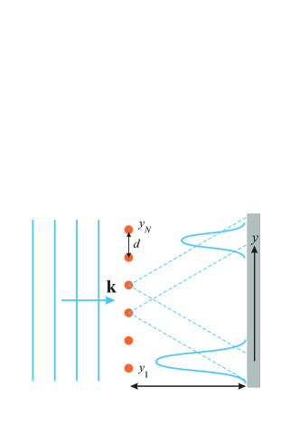
Figure 2: Schematic plot of electron scattering by a diffraction grating. Only the principal peaks are shown. The presented asymmetry corresponds to asymmetric scattering in Fig. 1.

In this geometry, we assume that each dot is an independent scatterer of the incoming plane wave with spin polarization along axis $x$. The distance $d$ between neighboring dots is of the order of electron wavelength $\lambda$, and we are observing the diffraction pattern at a relatively large distance $L\gg\lambda$. To consider the grating as a chain of independent scatterers, we first formulate the scattering independence condition:

$$\frac{R}{d}\left|{\bm{f}}\left({\pi}/{2}\right)\right|^{2}\ll\frac{l}{4}$$ (48)

meaning that the wave scattered by one dot cannot be re-scattered by its neighbors.

The scattering pattern produced at points $\left(L,y\right)$ on the screen is given by BornWolf :

$$\mathbf{F}{(y)}=\sum_{i=1}^{N}{\bm{f}}(\varphi_{i})\,\frac{e^{ikr_{i}}}{\sqrt{r_{i}}},$$ (49)

where $r_{i}=\sqrt{\left(y-y_{i}\right)^{2}+L^{2}}$ and $\varphi_{i}=\arctan(\left(y-y_{i}\right)/L).$ Then, we obtain the scattering density $\left|\mathbf{F}{(y)}\right|^{2}$ and density of spin components $\sigma_{j}(y)=\mathbf{F}^{{\dagger}}(y)\sigma_{j}\mathbf{F}{(y)}.$

The points, where the scattered waves produce constructive interference are determined by the constructive interference condition, $d\sin\varphi=n\lambda.$ For asymmetric scattering this relation also determines the spin orientation in the diffraction spots. The whole diffraction picture is asymmetric as the ”brightness” of spots is more pronounced in one of $\varphi$-directions (this is shown in Fig. 5 as a larger peak for $\varphi<0$ than for $\varphi>0$, in accordance with Fig. 1). Thus, we obtain scattering profile corresponding to $|{f}\left(\varphi\right)|^{2}$ with asymmetric scattering pattern. This asymmetric profile corresponds to formation of the spin current also.

Now we turn to the diffraction picture for the spin polarization where the qualitative feature is the emergence of nonzero $z-$axis spin polarization. To clarify this effect we consider two-dots realization with $N=2,$ $y_{1}=-d/2,$ and $y_{2}=d/2,$ where

$$\mathbf{F}{(y)}={\bm{f}}(\varphi_{1})\,\frac{e^{ikr_{1}}}{\sqrt{r_{1}}}+{\bm{f}}(\varphi_{2})\,\frac{e^{ikr_{2}}}{\sqrt{r_{2}}},$$ (50)

with

$$r_{1,2} = \overline{r}+\Delta r_{1,2}=\overline{r}\pm\frac{d}{2}\frac{y}{\sqrt{L^{2}+y^{2}}},$$ (51)

$$\varphi_{1,2} = \overline{\varphi}+\Delta\varphi_{1,2}=\overline{\varphi}\pm\frac{d}{2}\frac{L}{L^{2}+y^{2}},$$ (52)

where $\overline{r}=\sqrt{L^{2}+y^{2}}$ and $\overline{\varphi}=\arctan(y/L).$ Expansions in Eq. (50) with small $|\Delta r|\ll L$ and $|\Delta\varphi|\ll|\overline{\varphi}|\sim 1,$ show for the scattering density:

$$\left|\mathbf{F}{(y)}\right|^{2}\approx\frac{4}{\overline{r}}\cos^{2}\left(k\Delta r\right)\left|{\bm{f}}(\overline{\varphi})\right|^{2}$$ (53)

and for the $z-$component of spin:

$$\mathbf{F}^{{\dagger}}(y)\sigma_{z}\mathbf{F}{(y)}=\left|{F}^{\uparrow}(y)\right|^{2}-\left|{F}^{\downarrow}(y)\right|^{2}$$

$$\approx -\frac{1}{\overline{r}}\sin\left(k\Delta r\right)\Delta\varphi|{\bm{f}}(\overline{\varphi})|^{2},$$

where $\Delta{r}=\Delta{r}_{2}-\Delta{r}_{1}$ and $\Delta\varphi=\Delta\varphi_{2}-\Delta\varphi_{1}.$ Since $k\Delta r=2\pi({d}/{\lambda})\times{y}/\sqrt{L^{2}+y^{2}}$ at $d\ll\,L$ is much larger than $\Delta\varphi,$ the scattering intensity weakly depends on $\Delta\varphi.$ The resulting $\mathbf{F}^{{\dagger}}(y)\sigma_{z}\mathbf{F}{(y)}$ is not zero but rapidly decreases with $y.$

VI Numerical results: cross-section and scattering angles

VI.1 Single scatterers

The results of numerical calculations of the scattering cross-section length $l/R,$ mean angle $\langle\varphi\rangle$ and dispersion $D_{\varphi}$ based on Eqs. (28) and (29) are presented in Fig. 3 as the universal functions of parameters $\epsilon$ and $M$.

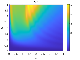
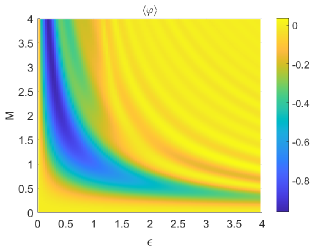
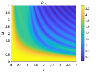
Figure 3: Numerical results for $l/R$, $\langle\varphi\rangle,$ and $D_{\varphi},$ as marked above the plots. In all numerical calculations we use $\hbar v=2.5\times 10^{2}$ meVnm with $v=4\times 10^{7}$ cm/s typical for Bi-based topological insulators Liu2010 , $\Delta_{\rm m}=25$ meV and consider $-10\leq m\leq 10$ harmonics. We emphasize that the results in terms of $M$ and $\epsilon$ parameters are universal and do not depend on the choice of these numerical values.

The upper panel shows that the ratio $l/R$ is small both for small $M,$ corresponding to the Born approximation and for relatively large $M$ and $\epsilon,$ where electron energy is sufficient to ensure a relatively weak effect of the nanosize dot on the electron propagation.

The mean scattering angle in the middle panel is typically small since the scattering is still close to $\varphi\leftrightarrow\,-\varphi$ symmetric in the domain of $\epsilon\sim 1$ and $M>1/2.$ Also, at large energies the forward scattering dominates leading to a small mean $|\langle\varphi\rangle|\ll 1.$

On the contrary, $D_{\varphi}$ is relatively large at $M<1$ being of the order of one and then decreases since the forward scattering with $|\langle\varphi\rangle|\ll\,1$ and $\langle\varphi^{2}\rangle\ll\,1$ becomes dominating. Notice hyperbolic structure clearly seen at $M\epsilon>1$ in the mean scattering angle and its dispersion demonstrating a periodic dependence on $M\epsilon$ product with the $\pi/2$ period, corresponding to Eq. (47).

To illustrate this behavior of the cross-section and scattering angle, we plot in Fig. 4 the angular dependence of the differential scattering cross-section. Figure 4 shows that at small energies this function behaves as $\sin^{2}(\varphi/2)$ and with the increase in the energy the scattering becomes less symmetric till it becomes mainly forward at high energies. At higher energies and larger $M,$ one obtains forward scattering with a relatively weak asymmetry $|\langle\varphi\rangle|\ll\,1$ and small aperture $D_{\varphi}\ll\,1.$

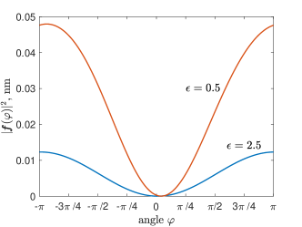
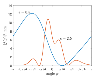
Figure 4: Differential cross-section length of electron scattering of magnetic quantum dot for different electron energies (as marked near the plots). Upper panel corresponds to $R=2$ nm ($M=0.2$) and lower panel corresponds to $R=15$ nm ($M=1.5$). The system parameters are the same as in Fig. 3. Weak forward scattering at $M\ll\,1$ corresponds to the perturbation theory in the Born approximation Kudla2022 .

VI.2 Diffraction gratings

Having discussed single-dot scattering, here we present in Fig. 5 the numerical results for the density probability and spin density produced by a diffraction grating.

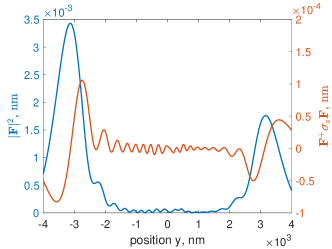
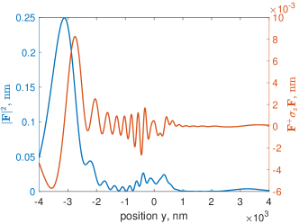
Figure 5: Scattering probability and spin density produced by nanodots-formed diffraction grating with $N=10$ dots, the interdot distance $d=150$ nm, and distance to the screen $L=2000$ nm. Upper panel corresponds to $R=5$ nm, lower panel corresponds to $R=15$ nm. Electron energy $\varepsilon=\Delta_{\rm m}/2=12.5$ meV, wavevector $k=5\times\,10^{-2}$ nm${}^{-1},$ and the wavelength $\lambda=1.26\times\,10^{2}$ nm. Scattering angle $\varphi$ for the first principal maxima obtained with $d|\sin\varphi|=\lambda$ yields $|\sin\varphi|=\lambda/d=0.84$ and corresponds to position on the screen $|y|=L|\sin\varphi|/\sqrt{1-\sin^{2}\varphi}\approx\,3100$ nm, in agreement with the presented plots. Although Eqs. (53) and (V) are not directly applicable here, they agree with these results demonstrating small $\sigma_{z}(y)$ near the principal peaks maxima.

As shown in Fig. 5, the diffraction pattern consists of strong principal scattering peaks and of weak secondary intermediate peaks, as predicted by the diffraction theory BornWolf . As expected, the diffraction pattern is strongly asymmetric with $\langle\varphi\rangle<0,$ as can be understood from Figs. 3 and 4. In addition, we see that the $\sigma_{z}(y)$ spin density is small but not zero, as expected from the discussion above when for a single scatterer $\sigma_{z}(y)=0.$ Figure 5 shows that with the given gratings geometry one can achieve the spin polarization $\sigma_{z}(y)/\left|\mathbf{F}(y)\right|^{2}\leq 0.1.$ This is a result of interference of the waves scattered by different angles $\varphi_{i}$, similar to the effects observed in the scattering of bunches of ultrafast electrons in solids Michalik2008 .

VII Conclusions

We studied cross-section and diffraction patterns of electron scattering by magnetic nanodots and their diffraction gratings on the surface of a topological insulator with spin-momentum locking. For a single nanomagnet, we considered analytically and numerically various scattering regimes in terms of the electron energy and nanodot size and magnetization and demonstrated that they can be universally described by two dimensionless system parameters. The scattering probability is usually angle-asymmetric, presenting its qualitative feature due to the spin-momentum locking as can occur in a broad interval of the scattering angles. It becomes angle-symmetric (i) at high energies, where it is concentrated in a narrow angle and (ii) in the energy-independent Born approximation leading to the universal broad scattering probability distribution. We demonstrated that the spins of scattered electrons remain parallel to the surface of the topological insulator. Next, we obtained the corresponding patterns of the scattering by diffraction gratings. In qualitative contrast to single scatterers, diffraction gratings produce nonzero perpendicular to the surface spin component of the scattered electrons.

These results can be applied for the design of magnetization patterns such as arrays of magnetic quantum dots or magnetization lattices of nanomagnets of the size between 10 and 100 nm Cowburn1999 to produce in a controllable way spin and charge currents and densities at the surfaces of topological insulators. This approach can be used for studies of spin torques Mellnik2014 ; Ndiaye2017 ; Han2017 ; Ghosh2017 ; Bondarenko2017 ; Mahendra2018 ; Moghaddam2020 ; Han2021 produced on the magnetized quantum dots by scattered electrons. Another application can be related to electron interferometry and holography of magnetic structures and nonuniform magnetic fields Fukuhara1983 ; Tonomura1987 providing detailed information about magnetization patterns by visualization of the phase of the electron wavefunction.

References

- (1) Yu.A. Bychkov and E.I. Rashba, Properties of a 2D electron gas with a lifted spectrum degeneracy, Sov. Phys. - JETP Lett. 39, 78 (1984).
- (2) M. Z. Hasan and C. L. Kane, Colloquium: Topological insulators, Rev. Mod. Phys. 82, 3045 (2010).
- (3) X.-L. Qi and S.-C. Zhang, Topological insulators and superconductors, Rev. Mod. Phys. 83, 1057 (2011).
- (4) L. Fu, Hexagonal Warping Effects in the Surface States of the Topological Insulator Bi2Te3, Phys. Rev. Lett. 103, 266801 (2009).
- (5) T. Yokoyama, Current-induced magnetization reversal on the surface of a topological insulator, Phys. Rev. B 84, 113407 (2011).
- (6) J. Mochida and H. Ishizuka, Skew scattering by magnetic monopoles and anomalous Hall effect in spin-orbit coupled systems, arXiv:2211.10180 [cond-mat.mes-hall].
- (7) S. Hikami, A.I. Larkin, and Y. Nagaoka, Spin-Orbit Interaction and Magnetoresistance in the Two Dimensional Random System, Progr. Theor. Phys. 63, 707 (1980).
- (8) S. Kudła, A. Dyrdał, V. K. Dugaev, J. Berakdar, and J. Barnaś, Conduction of surface electrons in a topological insulator with spatially random magnetization, Phys. Rev. B 100, 205428 (2019).
- (9) F. Katmis, V. Lauter, F. S. Nogueira et al., A high-temperature ferromagnetic topological insulating phase by proximity coupling, Nature 533, 513 (2016).
- (10) Y. Tokura, K. Yasuda, and A. Tsukazaki, Magnetic topological insulators, Nature Reviews Physics 1 126, (2019).
- (11) M. Jamali, J. S. Lee, J. S. Jeon et al., Giant Spin Pumping and Inverse Spin Hall Effect in the Presence of Surface and Bulk Spin Orbit Coupling of Topological Insulator Bi2Se3, Nano Lett. 15, 7126 (2015).
- (12) T. Chiba, S. Takahashi, and G. E. W. Bauer, Magnetic-proximity-induced magnetoresistance on topological insulators, Phys. Rev. B 95, 094428 (2017).
- (13) W. Chen, Edelstein and inverse Edelstein effects caused by the pristine surface states of topological insulators, J. Phys. Condens. Matter 32, 035809 (2020).
- (14) L. P. Rokhinson, V. Larkina, Y. B. Lyanda-Geller, L. N. Pfeiffer, and K. W. West, Spin Separation in Cyclotron Motion, Phys. Rev. Lett. 93, 146601 (2004).
- (15) M. J. Rendell, S. D. Liles, A. Srinivasan, O. Klochan, I. Farrer, D. A. Ritchie, and A. R. Hamilton, Gate voltage dependent Rashba spin splitting in hole transverse magnetic focusing, Phys. Rev. B 105, 245305 (2022).
- (16) J. Hutchinson and J. Maciejko, Universality of low-energy Rashba scattering, Phys. Rev. B 96, 125304 (2017).
- (17) E.I. Rashba, Spin currents, spin populations, and dielectric function of noncentrosymmetric semiconductors, Phys. Rev. B 70, 161201 (2004).
- (18) I.V. Tokatly and E.Ya. Sherman, Gauge theory approach for diffusive and precessional spin dynamics in a two-dimensional electron gas, Annals of Physics 325, 1104 (2010).
- (19) M.I. Dyakonov and V.I. Perel’, Current-induced spin orientation of electrons in semiconductors, Phys. Lett. A 35, 459 (1971).
- (20) J. Sinova, D. Culcer, Q. Niu, N.A. Sinitsyn, T. Jungwirth, and A.H. MacDonald, Universal Intrinsic Spin Hall Effect, Phys. Rev. Lett. 92, 126603 (2004).
- (21) S. Murakami, N. Nagaosa, and S.-C. Zhang, Dissipationless Quantum Spin Current at Room Temperature, Science 301, 1348 (2003).
- (22) Y.K. Kato, R.C. Myers, A.C. Gossard, and D.D. Awschalom, Observation of the spin Hall effect in semiconductors, Science 306, 1910 (2004).
- (23) E.G. Mishchenko, A.V. Shytov, and B.I. Halperin, Spin Current and Polarization in Impure Two-Dimensional Electron Systems with Spin-Orbit Coupling, Phys. Rev. Lett. 93, 226602 (2004).
- (24) V. Sih, R.C. Myers, Y.K. Kato, W.H. Lau, A.C. Gossard, D.D. Awschalom, Spatial imaging of the spin Hall effect and current-induced polarization in two-dimensional electron gases, Nature Physics 1, 31 (2005).
- (25) J. Wunderlich, B. Kaestner, J. Sinova, and T. Jungwirth, Experimental Observation of the Spin-Hall Effect in a Two-Dimensional Spin-Orbit Coupled Semiconductor System, Phys. Rev. Lett. 94, 047204 (2005).
- (26) A. R. Mellnik, J. S. Lee, A. Richardella et al., Spin-transfer torque generated by a topological insulator, Nature 511, 449 (2014).
- (27) P. B. Ndiaye, C. A. Akosa, M. H. Fischer et al., Dirac spin-orbit torques and charge pumping at the surface of topological insulators, Phys. Rev. B 96, 014408 (2017).
- (28) J. Han, A. Richardella, S. A. Siddiqui et al., Room-Temperature Spin-Orbit Torque Switching Induced by a Topological Insulator, Phys. Rev. Lett. 119, 077702 (2017).
- (29) S. Ghosh and A. Manchon, Spin-orbit torque in a three-dimensional topological insulator – ferromagnet heterostructure: Crossover between bulk and surface transport, Phys. Rev. B 97, 134402 (2018).
- (30) D.C. Mahendra, R. Grassi, J.-Y. Chen et al., Room-temperature high spin–orbit torque due to quantum confinement in sputtered BixSe1–x films, Nature Materials 17, 800 (2018).
- (31) A. G. Moghaddam, A. Qaiumzadeh, A. Dyrdał, and J. Berakdar, Highly Tunable Spin-Orbit Torque and Anisotropic Magnetoresistance in a Topological Insulator Thin Film Attached to Ferromagnetic Layer, Phys. Rev. Lett. 125, 196801 (2020).
- (32) J. Han and L. Liua, Topological insulators for efficient spin–orbit torques, APL Materials 9, 060901 (2021).
- (33) P. V. Bondarenko and E. Ya. Sherman, Uniform magnetization dynamics of a submicron ferromagnetic disk driven by the spin–orbit coupled spin torque, J. Phys. D: Appl. Phys. 50, 265004 (2017).
- (34) R. G. Newton Scattering Theory of Waves and Particles: Second Edition, Dover Books on Physics, New York (2013).
- (35) N. N. Lebedev, Special Functions and Their Applications, Dover Books on Mathematics, New York (1972).
- (36) W. R. Smythe Static and Dynamic Electricity, Taylor & Francis, New York (1989).
- (37) N. Nagaosa, J. Sinova, S. Onoda, A. H. MacDonald, and N. P. Ong, Anomalous Hall effect, Rev. Mod. Phys. 82, 1539 (2010).
- (38) S. Kudła, S. Wołski, T. Szczepański, V.K. Dugaev, and E.Ya. Sherman, Electron scattering by magnetic quantum dot in topological insulator, Solid State Commun. 342, 114555 (2022).
- (39) L.D. Landau and E.M. Lifshitz, Quantum Mechanics (Non-Relativistic Theory), Butterworth-Heinemann, Oxford (1981).
- (40) M. Born and E. Wolf, Principles of Optics: Electromagnetic Theory of Propagation, Interference and Diffraction of Light, Cambridge University Press (1999).
- (41) C.-X. Liu, X.-L. Qi, H. J. Zhang, X. Dai, Z. Fang, and S.-C. Zhang, Model Hamiltonian for topological insulators, Phys. Rev. B 82, 045122 (2010).
- (42) A. M. Michalik, E. Ya. Sherman, and J. E. Sipe, Theory of ultrafast electron diffraction: The role of the electron bunch properties, Journ. of Appl. Phys. 104, 054905 (2008).
- (43) R. P. Cowburn, D. K. Koltsov, A. O. Adeyeye, M. E. Welland, and D. M. Tricker, Single-Domain Circular Nanomagnets, Phys. Rev. Lett. 83, 1042 (1999).
- (44) A. Fukuhara, K. Shinagawa, A. Tonomura, and H. Fujiwara, Electron holography and magnetic specimens, Phys. Rev. B 27, 1839 (1983).
- (45) A. Tonomura, Applications of electron holography, Rev. Mod. Phys. 59, 639 (1987).