Language-Guided Generation of Physically Realistic Robot Motion and Control

Abstract

We aim to control a robot to physically behave in the real world following any high-level language command like “cartwheel” or “kick”. Although human motion datasets exist, this task remains particularly challenging since generative models can produce physically unrealistic motions, which will be more severe for robots due to different body structures and physical properties. In addition, to control a physical robot to perform a desired motion, a control policy must be learned. We develop LAnguage-Guided mOtion cONtrol (LAGOON), a multi-phase method to generate physically realistic robot motions under language commands. LAGOON first leverages a pretrained model to generate human motion from a language command. Then an RL phase is adopted to train a control policy in simulation to mimic the generated human motion. Finally, with domain randomization, we show that our learned policy can be successfully deployed to a quadrupedal robot, leading to a robot dog that can stand up and wave its front legs in the real world to mimic the behavior of a hand-waving human. Project website: https://sites.google.com/view/lagoon-text2control

1 Introduction

Thanks to the recent advances in foundation models [10, 5, 43], natural language has become a universal interface for a wide range of AI applications. A well-trained generative model can produce highly complex data conditioning on any human language description. Representative successes include generating images [45, 44, 48], videos [58], programming languages [9, 11], game playing strategies [66], and even robotic action primitives [1, 12].

A similar trend also emerges in motion generation to develop motion generative models conditioning on specified language commands [61]. The key idea is to leverage a pretrained language embedding model [43] to encode the commands and then train a generative model [20, 59, 60] to produce high-quality motions, leading to interesting applications such as creating animation or human-scene interactions [55, 64, 22, 78]. However, a common pitfall of these works is that the generated motion may often violate real-world physical constraints since no physics simulation is performed during such an end-to-end generation process. This issue can be even more severe for generating robot motions since most existing motion datasets are collected from human demonstrators while a robot can have a drastically different body structure from humans.

An alternative paradigm is to leverage reinforcement learning (RL) to directly learn a physically realistic control policy [38, 41]. Since the RL policy is trained in a physics engine, the produced motion from the control policy must satisfy all the physics constraints. Furthermore, with advanced sim-to-real training techniques [39], the learned policy can be transferred to a real robot for physical-world behavior. However, effective RL training often requires a heavily engineered reward function [49], which becomes infeasible for language-guided generation.

In this work, we aim to generate physically realistic motion and control for any high-level language description by leveraging the benefits from both end-to-end generation and RL training. We developed a multi-phase method LAnguage-Guided mOtion cONtrol (LAGOON). LAGOON first adopts a motion diffusion model to generate a human motion from the language description. The generated human motion is mapped to a robot body to create a semantically desired but physically unrealistic target robot motion. Then an RL phase is performed to learn a policy in a physics engine to control a robot to mimic the target motion. Finally, with domain randomization, we show that the learned RL policy can be deployed to a real-world robot.

We emphasize that effectively training an RL policy to mimic the target motion is nontrivial in our setting. Although there exist algorithms that can learn motion control from demonstration videos, these works typically assume perfect demonstrations from human professionals [50, 54, 76, 53]. By contrast, the target motion in our setting is completely synthetic and can be highly unrealistic. The generated motion may contain physically impossible poses or even missing frames, resulting in teleportation or floating behaviors. We adopt a special reward design for motion imitation, which combines both adversarially learned critic reward for high-level semantic consistency and an optimal-matching-based state-error reward to enforce fine-grained consistency to critical frames from the target motion.

We evaluate LAGOON for two kinds of robots in simulation, i.e., a humanoid robot, which resembles the human body structure so that the generated target motion can be easier to mimic, and a quadrupedal robot, which has a completely different body structure leading to more challenges for RL training. We empirically show that LAGOON can generate robust control policies for both robots to produce physically realistic behaviors following various language commands. For the humanoid robot, LAGOON produces qualitatively better motions than the baselines on high-level commands like “cartwheel” as well as commands requiring fine-grained control like “kick”. We also conduct quantitative analysis by measuring different motion statistics, where LAGOON consistently outperforms all the RL baselines. For the quadrupedal robot, despite the substantial differences in body structure, LAGOON is able to produce a policy to execute the language command “throw a ball” by controlling the robot to stand up and wave its front legs, just like a human. Finally, we successfully deployed our learned policy to a physical quadrupedal robot, resulting in a standing robot dog waving its “hands” in the real world.

2 Related work

2.1 Motion Generation

Motion generation is of great importance in computer graphics and related domains. Motion synthesis methods can be broadly divided into two categories: unconstrained generation [67, 79] and conditioned synthesis. Conditioned generation methods aim for controllability using music [26, 27, 28], speech [7, 17], or language. We consider language-conditioned motion generation. Early works on translating text description to human motion adopt a deterministic encoder-decoder architecture [2, 16]. Since motions in nature are stochastic, recent works have started to use deep generative models such as GANs, VAEs [18, 42], or diffusion models [47, 61, 77] to generate motions. Note that these motion generation methods are trained on large motion datasets and are typically limited to human motion generation.

Despite their superior performances, standard deep generative models do not explicitly incorporate the law of physics into the generation process. [46, 56, 68] adopt physics-based motion optimization to adjust the body positions and orientations. Other works adopt motion imitation in the physical simulator to estimate human pose from optical non-line-of-sight imaging system [23], sparse inertial sensors [68], and videos [71, 72, 31, 32, 75]. [74] integrate the imitation policy trained in a physics simulator into the sampling process of the diffusion model. However, most of these works [56, 31, 75, 32, 68, 74] still rely on a manually designed residual force [73] at the root joint to compensate for the dynamics mismatch between the physics model and real humans, which does not apply to real robot control.

2.2 Learning Methods for Robot Control

In order to achieve more naturalistic behaviors, researchers carefully design heuristics for symmetry [70], energy consumption [4], and correct contact with the environment [37]. However, such methods typically require significant domain expertise and thus are limited to simple tasks. Imitation learning (IL) is a more general approach, which can learn from expert demonstrations and deploy the learned policy in physics simulators [38, 6, 41] or the real world [40, 14]. IL assumes perfect data from the real world, while we only have access to imperfect synthetic demonstrations. Some works leverage pre-trained models to control robots. For example, a language model can be adopted for representation learning [57] or semantic planning [1]. However, these works require human demonstrations of low-level control while we do not require any additional control data. [3, 12] train a video diffusion model to generate a sequence of trajectory states and use inverse dynamics to infer the actions. In our setting, the reference motion and the actual rollout policy trajectory cannot be precisely aligned. Therefore, it is infeasible to produce actions through inverse dynamics.

2.3 State-Based Imitation Learning

It can be often the case that expert actions are unavailable, and the policy must learn from states. One approach is to learn a dynamics model to infer actions from state transitions and then apply behavior cloning [62, 13]. Other works directly perform RL with a state-based imitation reward, such as differences between states representations [6, 38, 54, 76], or an adversarially learned discriminator [35, 63, 24, 41, 29, 15, 65]. We leverage both two rewards to train our RL policy. Since the policy motion and the reference motion can be largely mismatched in our setting, both reward terms are critical for the empirical success.

2.4 Quadrupedal Motion and Control

Previous approaches have focused on generating controllable or natural quadrupedal motions and gaits either by imitating animals [40] or by relying on heavily engineered reward functions [34, 49]. Our work demonstrates the ability to generate diverse motions without the need for domain-specific data or meticulously designed reward functions.

3 Preliminary

We consider a robot control problem following language commands. The aim is to derive a control policy $\pi$ conditioned on language command $c$.

3.1 Human Motion Generation

Human motion generation aims to a sequence $x_{0:H}=\{x_{h}\}_{h=0}^{H}$. Each frame $x_{h}\in\mathbb{R}^{J\times K}$ represents a human pose using $K$-dimensional features of $J$ joints. Here $K$-dimensional features can be either the joint angles or positions. Given a language command $c$, a language-conditioned motion generation model aims to generate a motion matching the description $c$.

Recently, diffusion models [20, 59, 60] can generate high-quality human motion [47, 61, 77]. They model the data distribution by gradually injecting noises into the data distribution and gradually denoise a sample from a Gaussian distribution. The forward diffusion process injects i.i.d. Gaussian noises, namely

$$x_{0:H}^{l}\sim\mathcal{N}(\sqrt{\alpha_{l}}x_{0:H}^{l-1},(1-\alpha_{l})\mathbf{I}),$$

where $x_{0:H}^{0}$ denotes samples drawn from the real data distribution $p^{0}(x^{0})$. For large enough $l$, $x_{0:H}^{l}$ approximately follows the Gaussian distribution $\mathcal{N}(\mathbf{0},\mathbf{I})$. A denoiser $F_{d}(x^{l},l)$ is trained to gradually denoise $x_{0:H}^{l}$ back to $x_{0:H}^{l-1}$. The training objective of $F_{d}$ is usually given by

$$\mathbb{E}_{x^{0}\sim p^{0}(x^{0}),l\sim q(l),\epsilon\sim\mathcal{N}(\mathbf{0},\mathbf{I})}\left[\lambda(l)\|x^{0}-F_{d}(x^{l},l)\|^{2}\right],$$

where $q(l)$ is a distribution from which $l$ is samapled and $\lambda(l)$ is a weighting factor.

3.2 RL for Control

Rather than generating a motion directly, RL methods learn a policy in simulation to control a robot to perform the desired motion according to some given reward function.

3.2.1 Markov Decision Process

The robot control problem can be formulated as a Markov Decision Process (MDP) denoted by $M=\langle\mathcal{S},\mathcal{A},\mathcal{T},r,\gamma\rangle$. Here $\mathcal{S}$ is the state space, and $\mathcal{A}$ is the action space. $\mathcal{T}:\mathcal{S}\times\mathcal{A}\times\mathcal{S}\to[0,1]$ is the transition function. $\mathcal{T}(s^{\prime}|s,a)$ denotes the probability of reaching a state $s^{\prime}$ from a state $s$ under an action $a$. $r:\mathcal{S}\times\mathcal{A}\to\mathbb{R}$ is the reward function and $\gamma$ is the discounted factor. In our task setup, the reward function $r$ is generated based on a language command $c$. In practice, when applying RL for robot control, complex reward designs are often required due to a lot of motor joints and movement constraints [49].

At each time step $t$, the control policy produces an action $a_{t}\sim\pi(\cdot|s_{t})$, and receives a reward $r(s_{t},a_{t})$. The objective of RL is to find the optimal policy $\pi^{\star}$ that could maximize the discounted accumulated reward,

$$\pi^{\star}=\arg\max_{\pi}\mathbb{E}\left[\sum_{t\geq 0}\gamma^{t}r(s_{t},a_{t})\mid a_{t}\sim\pi\left(\cdot\mid s_{t}\right),s_{0}\right].$$

where $s_{0}$ is the initial state.

3.2.2 Proximal Policy Optimization

Proximal Policy Optimization (PPO) [52] is one of the most widely-used on-policy RL algorithms. PPO adopts the actor-critic architecture and learns a policy $\pi_{\theta}$ parameterized by $\theta$ and a value function $V_{\phi}(s)$ parameterized by $\phi$, which is utilized to estimate the value of the states,

$$V_{\phi}(s)=\mathbb{E}\left[\sum_{t\geq 0}\gamma^{t}r(s_{t},a_{t})\mid a_{t}\sim\pi_{\theta}(\cdot\mid s_{t}),s_{0}=s\right]$$

PPO maximizes the following objective,

$$L^{\mathrm{CLIP}}(\theta)=\\ \mathbb{E}_{t}\left[\min\left(\alpha_{t}(\theta)\hat{A}_{t},\operatorname{clip}\left(\alpha_{t}(\theta),1-\epsilon,1+\epsilon\right)\hat{A}_{t}\right)\right]$$

where $\alpha_{t}(\theta)=\frac{\pi_{\theta}\left(a_{t}\mid s_{t}\right)}{\pi_{\theta_{\text{old }}}\left(a_{t}\mid s_{t}\right)}$ denotes the importance ratio. $\epsilon$ controls trust region. $\hat{A}_{t}$ estimates $A_{t}=R_{t}-V_{\pi_{\theta}}(s_{t})$, where $R_{t}=\sum_{t^{\prime}\geq t}\gamma^{t^{\prime}-t}r(s_{t^{\prime}},a_{t^{\prime}})$ is the discounted return.

3.2.3 RL-Based Motion Imitation

Our goal is to derive an RL policy given a language command $c$. However, it is difficult to design reward functions directly for robot control tasks. One approach to solving this problem is imitation learning (IL), which is also called learning from demonstration. In imitation learning, we assume that there is a dataset $\mathcal{D}=\{(s_{i},a_{i})\}_{i=1}^{m}$ collected by an expert or reference policy $\pi_{E}$. The goal of IL is to find the optimal policy $\pi^{*}$ that covers the distribution of state-action pairs in the dataset $\mathcal{D}$. Two typical approaches are behavior cloning [19] and inverse reinforcement learning [8], which match state-action pairs between the expert and the imitator. We are interested in cases where expert actions are not available and the dataset only contains a trajectory of states, i.e. $\mathcal{D}=\{x_{i}\}_{i=0}^{H}$. One approach to solve this problem is state-based IL [35, 38, 41]. State-based IL typically designs a state-error reward [38], which encourages the imitator to reach the reference states $x_{0:H}$. Let $s_{t}$ denote the imitator state at timestep $t$, the state-error reward $r^{\mathrm{err}}_{t}$ can be defined as,

$$r^{\mathrm{err}}_{t}=Sim(x_{t},s_{t})$$ (1)

where $Sim(x_{t},s_{t})$ represents the similarity between the reference state $x_{t}$ and the imitator state $s_{t}$ at timestep $t$.

A crucial assumption of state-based IL is a strict timing alignment between the demonstration and the rollout trajectory, i.e. the agent receives a high reward at timestep $t$ if and only if $s_{t}$ is close to $x_{t}$. This can be problematic when the reference motion $x_{0:H}$ is not physically realistic. Adversarial imitation learning (AIL) tackles this issue by training a discriminator $D_{\psi}$ to differentiate behaviors generated by the imitator from the reference motion $x_{0:H}$, where $\psi$ is the network parameters. The discriminator then scores the states $s_{t}$ generated by the imitator. Specifically, a discriminator $D_{\psi}$ is trained to discriminate between state transitions in the reference motion and the samples generated by the current policy $\pi_{\theta}$:

$$\mathcal{L}_{\text{disc}}=\mathbb{E}_{h}[-\log D_{\psi}(x_{h},x_{h+1})]\\ +\mathbb{E}_{t}[-(1-\log D_{\psi}(s_{t},s_{t+1}))]+w_{\text{gp}}\mathcal{L}_{\text{gp}},$$

where $\mathcal{L}_{\text{gp}}$ is a gradient penalty term given by

$$\mathcal{L}_{\text{gp}}=\mathbb{E}_{h}[\|\nabla_{(x_{h},x_{h+1})}D_{\psi}(x_{h},x_{h+1})\|^{2}].$$

As discussed in [36], this zero-centered gradient penalty stabilizes training and helps convergence. AIL optimizes the policy $\pi_{\theta}$ to maximize the discounted accumulated adversarial reward. The adversarial reward is given by,

$$r^{\mathrm{adv}}_{t}=-\log(1-D_{\psi}(s_{t-1},s_{t})).$$ (2)

4 Methodology

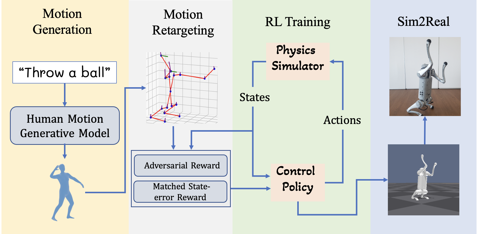
Figure 1: Overview of the multi-phase method LAnguage-Guided mOtion cONtrol (LAGOON). To train a robust policy that controls the robot following a language command such as “throw a ball”, we first generate a human motion using the motion generation model. Then the human motion can be retargeted to a robot skeleton that differs largely from humans (i.e., the quadrupedal robot). By introducing RL training, we train a robust control policy with a combinational reward in the physics simulator. Finally, we deploy the control policy to the real-world robot via domain randomization.

As shown in Fig. 1, we derive a robot control policy following a language command $c$ through a multi-phase method. We first generate a motion sequence $x_{0:H}$ conditioned on $c$ using a human motion generation model. $x_{0:H}$ is then retargeted to the robot skeleton to produce a robot motion $y_{0:H}$. Finally, we adopt RL training to obtain a control policy $\pi_{\theta}$ and transfer the learned policy to the real world via domain randomization.

4.1 Motion Generation and Motion Retargeting

In the motion generation stage, we adopt a SOTA Human Motion Diffusion Model (MDM) [61] to generate human motion $x_{0:H}$ conditioned on a language command $c$. Since MDM can only generate human motion, we then adopt a retargeting stage to map the human motion $x_{0:H}$ to the desired robot motion $y_{0:H}$. Taking the quadrupedal robot as an example, we map the human skeleton to the robot’s skeleton, with the human arms corresponding to the robot’s two front legs and the human legs corresponding to the robot’s two rear legs, and then retarget each joint and joint rotation. For the humanoid robot, the number of joints on different skeletons may vary and therefore also need to be retargeted accordingly. For those joints that are redundant, they are simply discarded. The mapping relations and more retargeting details are presented in Appendix.

4.2 RL Training

The RL phase trains a control policy $\pi_{\theta}$ to imitate the retargeted robot motion $y_{0:H}$. The policy takes in robot states and outputs an action to interact with the physics simulator. The reward is calculated by comparing the robot states with the retargeted reference robot motion. The motion generated by MDM is physics-ignoring, so floating, penetration and teleportation behaviors may often occur, which can be amplified in the retargeted robot motion $y_{0:H}$. Inaccurate reference motions pose significant challenges to motion imitation, which we tackle via a careful reward design.

4.2.1 Reward Design

We combine both the adversarial reward $r^{\mathrm{adv}}$ (Eq. (2)) and a variant of the state-error reward $r^{\mathrm{me}}$ (Eq. (3)). Intuitively, the adversarial reward is universal to capture high-level semantic consistency with the reference motion. However, we empirically observe that only using an adversarial reward can fail to match critical poses in the reference motion. For example, when given the command “kick”, the policy trained with the adversarial reward alone only learns to stand but fails to perform a kick. Hence, for more fine-grained body control, we additionally leverage a state-error reward, which can be nontrivial since the policy trajectory and the reference motion are not well aligned.

To tackle the temporal mismatch issue, we employ a matching algorithm between the policy rollout trajectories and the reference motion to find the best temporal alignment leading to the highest state-error reward. More specifically, let $y_{0:H}$ be the reference motion sequence and $\tau=(s_{0},s_{1},\ldots,s_{T})$ be a trajectory from the policy. We define a matching $M$ between $y_{0:H}$ and $\tau=(s_{0},s_{1},\ldots,s_{T})$ by

$$M=\{(u_{0:k},v_{0:k})\mid k\in\mathbb{N}_{+},\\ 0\leq u_{0}<u_{1}<\cdots<u_{k}\leq H,\\ 0\leq v_{0}<v_{1}<\cdots<v_{k}\leq T\}.$$

where $s_{v_{m}}$ is matched with $y_{u_{m}}$ for all $0\leq m\leq k$. Recall that $Sim(y_{i},s_{j})$ is a similarity measurement between the $i$-th motion state $y_{i}$ and the robot state $s_{j}$ at timestep $j$. We aim to find the optimal matching $M^{*}=(u^{*}_{0:k^{*}},v^{*}_{0:k^{*}})$ that maximizes the total similarity, namely

$$(u^{*}_{0:k^{*}},v^{*}_{0:k^{*}})=\operatorname*{arg\,max}_{(u_{0:k},v_{0:k})\in M}\sum_{m=0}^{k}Sim(y_{u_{m}},s_{v_{m}}),$$

which can be solved via dynamic programming. The optimal matching $M^{*}$ helps filter out unrealistic poses and allows the robot to smoothly transit between two consecutive motion frames. With the optimal matching $(u^{*}_{0:k^{*}},v^{*}_{0:k^{*}})$, the matched state-error reward is defined as

$$r^{\mathrm{me}}_{t}=\begin{cases}Sim(y_{u^{*}_{m}},s_{v^{*}_{m}}),&\mbox{if }t=v^{*}_{m}\in v^{*}_{0:k^{*}}\\ 0.&\mbox{if }t\notin v^{*}_{0:k^{*}}\end{cases}$$ (3)

Our final reward is a combination of adversarial reward and matched state-error reward.

$$r_{t}=\lambda_{\mathrm{adv}}r^{\mathrm{adv}}_{t}+\lambda_{\mathrm{me}}r^{\mathrm{me}}_{t}$$ (4)

where $\lambda_{\mathrm{adv}}$ and $\lambda_{\mathrm{me}}$ are weighting factors. We also remark that the adversarial reward remains critical since it provides much denser reward signals than the state-error reward.

4.2.2 PPO with Augmented Critic Inputs

We utilize PPO [52] for RL training, which adopts an actor-critic structure with two separate neural networks, i.e. a policy $\pi_{\theta}$ and a value function $V_{\phi}$. The critic is only used for variance reduction at training time, so we can input additional information not presented in robot states to the value network to accelerate training. In particular, given the trajectory $\tau$, the reference sequence $y$, and the optimal matching $M^{*}$, for each state $s_{t}$, we take the next future reference motion for $s_{t}$ from $M^{*}$ as the additional information to the critic. Such future information significantly improves training in practice. We also remark that similar techniques have been widely adopted in multi-agent RL [69].

4.2.3 More Implementation Details

Hybrid initial states: The initial states of the reference motion may differ significantly from the initial robot states. For example, the initial states of the reference motion $y_{0:H}$, which is retargeted from human motion $x_{0:H}$, are standing on two feet. By contrast, a quadrupedal robot stands on four feet, resulting in training difficulties. Therefore, we adopt hybrid initial states, i.e., half of the episodes start from the default initial state of the robot while the other half starts from the standing state from the reference motion.

Policy network: We adopt a parametrized Gaussian policy $\pi_{\theta}(a|s)=\mathcal{N}(\mu_{\theta}(s),\Sigma)$, where the mean action $\mu_{\theta}(s)$ is output by a multi-player perception (MLP) network, with parameters $\theta$, and $\Sigma$ is a fixed covariance matrix. More training details are listed in Appendix.

Robust control with domain randomization: In order to learn robust control policies, we adopt domain randomization [39] during RL training. We randomize both the terrains that the robot stands on as well as a few physics parameters in the simulator so that the trained RL policy can generalize to different terrain conditions and even to the real world. More details can be found in Appendix.

5 Experiment

We conduct experiments on the humanoid and quadrupedal robots in the IsaacGym [33] simulator. We test LAGOON using the 28 DoF humanoid from AMP [41, 33] and the go1 quadrupedal robot with 12 DoF. We use the target DoF angles of proportional derivative (PD) controllers as the actions. The action dimensions are 28 and 12 for the humanoid and quadrupedal robots, respectively. We illustrate the learned motions of both humanoid and quadrupedal robots. For the humanoid robot, we also compare LAGOON with various state-based imitation learning methods qualitatively and quantitatively. For the quadrupedal robot, we conduct an alation study on the techniques proposed in Sec.4.2.

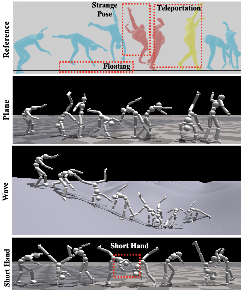
Figure 2: The reference motion sequence overlooks the law of physics. The trained policies robustly perform the “cartwheel” motion even in complex terrains (Wave) or a different skeleton with shorter arms (Short Hand).

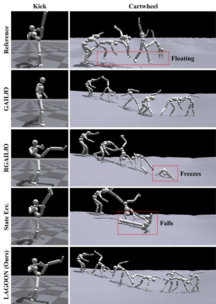
Figure 3: Comparision against the baselines trained with only adversarial rewards (GAILfO [63, 24, 41], RGAILfO [65]) or state-error rewards (State Err.). Adversarial rewards lack fine-grained motion tracking. Using state-error rewards alone would fail in complex tasks like doing cartwheels.

5.1 Humanoid Robot

For the humanoid robot, We conduct experiments on the tasks specified by the texts “the person runs backward”, “cartwheel”, and “the person kicks with his left leg”. These tasks include the movement and rotation of the entire body and fine-grained control of parts of the body.

Baselines

We compare LAGOON with other state-based imitation learning methods. BCO [62] is a non-RL method that learns an inverse dynamics model to label the reference motion with actions and adopt behavior cloning on the labeled motion. Other baselines are RL-based methods. State Err. only uses the state-error reward. GAILfO [63, 24, 41] and RGAILfO [65] utilize the adversarial rewards. In particular, RGAILfO tried to alleviate the problem of dynamics mismatch by introducing an adversary policy when collecting trajectories. We also conduct experiments using the hand-designed reward and denote it as pure RL. The reward for “run backward” is the backward velocity at each timestep. For the task “kick”, let $h_{t}$ denote the height of the robot’s left foot at timestep $t$, and the reward is computed as $\max(0,h_{t}-\max_{s<t}(h_{s}))$, which measure the difference between the current foot height and the previous maximum height. The “cartwheel” task is excluded since it is difficult to manually design reward functions for doing cartwheels.

Training Details

The input states of the control policy include the root’s linear velocity and angular velocity, the local velocity and rotation of each joint, and the 3D position of the end-effectors. We train the policies by randomizing the terrains and the physics parameters to handle various complex situations. There are four terrains during training. “Plane” refers to a flat surface without variations in elevation. “Rand.” is terrain with a bit of random undulation. “Pyramid” is square cone terrain with steps. “Wave” is the terrain with a great deal of undulation. We additionally train a policy for a humanoid robot with shorter arms.

We create 4096 parallel simulation environments in IsaacGym to collect training samples. The max episode length of each simulation is 300. Each environment would be reset when the robot in it falls (i.e., any part of the humanoid except hands and feet is in contact with the ground). We train the policy for 5,000 iterations and adopt the final policy for evaluation. All the RL-based baselines are trained using the same hyper-parameters. More details are listed in Appendix.

Method		LAGOON	GAILfO	RGAILfO	State Err.	Pure RL	BCO
Task: Cartwheel
Success Rate $\quad\uparrow$	Plane	$\mathbf{100.0\pm 0.0}$	$66.7\pm 47.1$	$0.0\pm 0.0$	$0.0\pm 0.0$	-	$0.0\pm 0.0$
	Rand.	$\mathbf{98.8\pm 0.5}$	$65.6\pm 46.3$	$6.3\pm 8.6$	$4.7\pm 6.6$	-	$0.0\pm 0.0$
	Pyramid	$\mathbf{85.2\pm 6.6}$	$33.1\pm 38.7$	$16.3\pm 22.7$	$15.0\pm 21.1$	-	$0.0\pm 0.0$
	Wave	$\mathbf{86.4\pm 10.6}$	$58.7\pm 34.7$	$19.9\pm 13.2$	$11.9\pm 15.3$	-	$0.0\pm 0.0$
	All Terr.	$\mathbf{92.6\pm 9.3}$	$56.0\pm 44.2$	$10.7\pm 15.9$	$7.9\pm 14.7$	-	$0.0\pm 0.0$
Episode Length $\quad\uparrow$	Plane	$\mathbf{300.0\pm 0.0}$	$298.5\pm 2.1$	$\mathbf{300.0\pm 0.0}$	$22.1\pm 2.3$	-	$7.1\pm 0.3$
	Rand.	$\mathbf{291.7\pm 2.2}$	$269.9\pm 15.6$	$202.3\pm 56.7$	$27.2\pm 4.9$	-	$7.9\pm 0.1$
	Pyramid	$206.3\pm 28.4$	$248.9\pm 35.7$	$\mathbf{260.1\pm 32.5}$	$32.9\pm 12.4$	-	$7.7\pm 0.5$
	Wave	$\mathbf{275.5\pm 18.2}$	$268.9\pm 17.8$	$255.9\pm 15.4$	$30.0\pm 8.9$	-	$7.7\pm 0.4$
	All Terr.	$268.4\pm 40.6$	$\mathbf{271.5\pm 27.8}$	$254.6\pm 48.3$	$28.0\pm 9.0$	-	$7.6\pm 0.5$
Direction Change $\quad\uparrow$	Plane	$\mathbf{1.9\pm 0.0}$	$1.7\pm 0.2$	$1.3\pm 0.0$	$0.8\pm 0.0$	-	$0.0\pm 0.0$
	Rand.	$\mathbf{1.9\pm 0.0}$	$1.7\pm 0.3$	$0.9\pm 0.3$	$0.7\pm 0.2$	-	$0.0\pm 0.0$
	Pyramid	$\mathbf{1.8\pm 0.1}$	$1.3\pm 0.5$	$1.3\pm 0.2$	$0.9\pm 0.3$	-	$0.0\pm 0.0$
	Wave	$\mathbf{1.7\pm 0.2}$	$1.5\pm 0.2$	$1.3\pm 0.1$	$0.7\pm 0.3$	-	$0.0\pm 0.0$
	All Terr.	$\mathbf{1.8\pm 0.1}$	$1.6\pm 0.3$	$1.2\pm 0.2$	$0.8\pm 0.3$	-	$0.0\pm 0.0$
Task: Kick
Success Rate $\quad\uparrow$	Plane	$\mathbf{100.0\pm 0.0}$	$0.0\pm 0.0$	$33.3\pm 47.1$	$\mathbf{100.0\pm 0.0}$	$100.0\pm 0.0$	$0.0\pm 0.0$
	Rand.	$\mathbf{78.9\pm 6.8}$	$46.6\pm 17.5$	$28.9\pm 18.9$	$75.3\pm 24.9$	$100.0\pm 0.0$	$0.0\pm 0.0$
	Pyramid	$\mathbf{89.9\pm 7.0}$	$60.4\pm 15.1$	$39.7\pm 14.2$	$85.4\pm 20.7$	$100.0\pm 0.0$	$0.0\pm 0.0$
	Wave	$69.7\pm 7.5$	$45.5\pm 8.3$	$29.5\pm 14.0$	$\mathbf{70.0\pm 29.2}$	$100.0\pm 0.0$	$0.0\pm 0.0$
	All Terr.	$\mathbf{84.6\pm 13.0}$	$38.1\pm 25.9$	$32.9\pm 27.6$	$82.6\pm 24.6$	$100.0\pm 0.0$	$0.0\pm 0.0$
Episode Length $\quad\uparrow$	Plane	$\mathbf{300.0\pm 0.0}$	$\mathbf{300.0\pm 0.0}$	$\mathbf{300.0\pm 0.0}$	$\mathbf{300.0\pm 0.0}$	$15.7\pm 3.1$	$6.3\pm 0.1$
	Rand.	$294.6\pm 3.9$	$\mathbf{299.5\pm 0.5}$	$298.7\pm 1.1$	$282.1\pm 21.0$	$17.1\pm 3.3$	$6.9\pm 0.1$
	Pyramid	$299.7\pm 0.1$	$185.9\pm 36.4$	$172.9\pm 28.3$	$\mathbf{299.9\pm 0.1}$	$16.1\pm 2.7$	$6.9\pm 0.2$
	Wave	$296.0\pm 3.1$	$298.0\pm 2.8$	$\mathbf{299.4\pm 0.7}$	$296.1\pm 5.3$	$17.7\pm 3.4$	$6.8\pm 0.3$
	All Terr.	$\mathbf{297.6\pm 3.4}$	$270.8\pm 52.3$	$267.8\pm 56.6$	$294.5\pm 13.1$	$16.6\pm 3.2$	$6.8\pm 0.3$
Height (m) $\quad\uparrow$	Plane	$1.3\pm 0.0$	$0.0\pm 0.0$	$0.4\pm 0.5$	$\mathbf{1.5\pm 0.0}$	$1.8\pm 0.0$	$0.1\pm 0.0$
	Rand.	$\mathbf{1.2\pm 0.1}$	$0.7\pm 0.2$	$0.6\pm 0.2$	$\mathbf{1.2\pm 0.3}$	$1.8\pm 0.0$	$0.1\pm 0.0$
	Pyramid	$\mathbf{1.3\pm 0.1}$	$1.1\pm 0.1$	$0.6\pm 0.1$	$\mathbf{1.3\pm 0.2}$	$1.8\pm 0.0$	$0.1\pm 0.0$
	Wave	$\mathbf{1.2\pm 0.0}$	$0.7\pm 0.1$	$0.6\pm 0.1$	$1.1\pm 0.4$	$1.8\pm 0.0$	$0.1\pm 0.0$
	All Terr.	$1.2\pm 0.1$	$0.6\pm 0.4$	$0.5\pm 0.3$	$\mathbf{1.3\pm 0.3}$	$1.8\pm 0.0$	$0.1\pm 0.0$
Task: Run Backwards
Success Rate $\quad\uparrow$	Plane	$\mathbf{100.0\pm 0.0}$	$\mathbf{100.0\pm 0.0}$	$\mathbf{100.0\pm 0.0}$	$\mathbf{100.0\pm 0.0}$	$97.2\pm 0.7$	$14.0\pm 0.5$
	Rand.	$99.8\pm 0.2$	$99.6\pm 0.4$	$\mathbf{99.9\pm 0.0}$	$99.1\pm 0.4$	$25.5\pm 2.1$	$13.6\pm 0.4$
	Pyramid	$\mathbf{100.0\pm 0.0}$	$99.9\pm 0.1$	$99.8\pm 0.3$	$\mathbf{100.0\pm 0.0}$	$96.6\pm 0.2$	$12.8\pm 0.9$
	Wave	$95.5\pm 1.2$	$96.2\pm 1.7$	$\bf{98.8\pm 0.5}$	$97.5\pm 1.0$	$24.0\pm 0.2$	$13.5\pm 0.9$
	All Terr.	$98.8\pm 2.0$	$98.9\pm 1.8$	$\mathbf{99.6\pm 0.6}$	$99.2\pm 1.1$	$60.8\pm 36.1$	$13.5\pm 0.8$
Episode Length $\quad\uparrow$	Plane	$\mathbf{300.0\pm 0.0}$	$\mathbf{300.0\pm 0.0}$	$\mathbf{300.0\pm 0.0}$	$\mathbf{300.0\pm 0.0}$	$299.8\pm 0.2$	$9.1\pm 0.1$
	Rand.	$299.4\pm 0.6$	$299.3\pm 0.8$	$\mathbf{299.8\pm 0.1}$	$298.8\pm 0.7$	$75.7\pm 6.8$	$9.5\pm 0.1$
	Pyramid	$\mathbf{299.9\pm 0.2}$	$299.6\pm 0.3$	$299.3\pm 0.9$	$\mathbf{299.9\pm 0.0}$	$298.7\pm 0.4$	$9.4\pm 0.1$
	Wave	$299.8\pm 0.3$	$\mathbf{300.0\pm 0.0}$	$\mathbf{300.0\pm 0.0}$	$\mathbf{300.0\pm 0.0}$	$62.6\pm 5.4$	$9.2\pm 0.2$
	All Terr.	$\mathbf{299.8\pm 0.4}$	$299.7\pm 0.5$	$\mathbf{299.8\pm 0.5}$	$299.7\pm 0.6$	$184.2\pm 115.2$	$9.3\pm 0.2$
Backward Distance (m) $\quad\uparrow$	Plane	$\mathbf{23.1\pm 1.4}$	$22.0\pm 1.5$	$22.2\pm 1.4$	$21.5\pm 0.8$	$65.4\pm 2.7$	$0.3\pm 0.0$
	Rand.	$18.7\pm 0.5$	$18.4\pm 1.0$	$19.6\pm 1.4$	$\mathbf{20.3\pm 0.9}$	$8.5\pm 1.9$	$0.3\pm 0.0$
	Pyramid	$26.8\pm 1.5$	$\mathbf{28.4\pm 1.9}$	$28.0\pm 1.5$	$21.7\pm 0.8$	$61.4\pm 2.2$	$0.3\pm 0.0$
	Wave	$17.4\pm 0.5$	$18.0\pm 1.5$	$20.3\pm 1.6$	$\mathbf{20.8\pm 1.0}$	$6.2\pm 0.5$	$0.3\pm 0.0$
	All Terr.	$21.5\pm 3.9$	$21.7\pm 4.4$	$\mathbf{22.5\pm 3.6}$	$21.1\pm 1.0$	$35.4\pm 28.2$	$0.3\pm 0.0$

Table 1: Success rates, episode lengths, and task-specific metric for the tasks on the humanoid. The success rate is the most direct measure to evaluate whether a model has successfully completed a given task. Episode length measures the stability of the policy since the episode is terminated when the robot falls. Plane, Rand, Pyramid, and Wave are different terrains. We train a single policy over all 4 terrains but evaluate the policies separately on each terrain. For each task and each terrain, the policies are evaluated on 4096 episodes over 3 different seeds. ”All Terr” represents the average across all four terrains.

5.1.1 Illustration of Learned Motion

A critical problem of the generated motion is physics ignoring. As shown in Fig. 2. The top picture is the motion generated by MDM conditioned on the language prompt “cartwheel”, where some postures are floating or ground-penetrating. We mark the strange postures impossible to imitate in red, and the posture represents that teleportation occurs in yellow. After retargeting and RL training, the control policy can do cartwheels in various scenarios. For example, the control policy can do cartwheels on a large slope after applying domain randomization. We also train the policy on the robot with short hands. We can observe that the robot can also do cartwheels steadily. Since these behaviors are conducted in the physics simulator, the generated robot motion would always be physically realistic.

5.1.2 Comparision with Baselines

Qualitative results

We compare LAGOON with various RL-based baselines. The results are shown in Fig. 3. The left column demonstrates policy behaviors in the “kick” task, and the right column demonstrates the “cartwheel” task. LAGOON complete both tasks successfully. The GAILfO policy tends to stick to a standing pose in the “kick” task, indicating that the fine-grained task is difficult to the adversarial rewards. The policy trained with only state-error reward fails to perform more complex skills like doing cartwheels. RGAILfO manages to complete both tasks with moderate performance. When doing cartwheels, the humanoid freezes, relying on both hands and feet for support.

Quantitative results

We also list the quantitative results in Tab. 1. We evaluate the policies on each task using three metrics. One is the episode length which measures the stability of the humanoid robot on different terrains. An episode is terminated if the robot falls, and we limit the max episode length to 300. We evaluate the success rates, and we also design a task-specific metric for each task. For the cartwheel task, we measure if the up axis of the humanoid has pointed downward and up again. Let $\mathbf{z}_{t}^{\text{up}}$ denote the up axis of the humanoid at time $t$ and let $\mathbf{\hat{z}}$ denote the global up axis ($\|\mathbf{z}_{t}^{\text{up}}\|=\|\mathbf{\hat{z}}\|=1$). We first compute $t_{\mathrm{low}}=\operatorname*{arg\,min}_{t}\mathbf{z}_{t}^{\text{up}}\cdot\mathbf{\hat{z}}$. The episode is considered successful if $\exists i<j,\mathbf{z}_{i}^{\text{up}}\cdot\mathbf{\hat{z}}<-0.7$ and $z_{j}^{\text{up}}\cdot\mathbf{\hat{z}}>0.7$. Our task-specific metric is given by $\max_{t\geq t_{\mathrm{low}}}\mathbf{z}_{t}^{\text{up}}\cdot\mathbf{\hat{z}}-\mathbf{z}_{t_{\mathrm{low}}}^{\text{up}}\cdot\mathbf{\hat{z}}$. For the kicking task, we evaluate the policies using the maximum height difference between the humanoid’s left and right feet. An episode is considered successful if the maximal height difference is at least 1. For the task of running backward, we compute the distance the humanoid travels in the backward direction. Specifically, let $\mathbf{v}_{t}$ denote the root velocity of the humanoid at time $t$ and let $\mathbf{d}_{t}^{h}$ denote the heading direction at time $t$ ($\|\mathbf{d}_{t}^{h}\|=1$). We use $\sum_{t}-(\mathbf{v}_{t}\cdot\mathbf{d}_{t}^{h})\Delta t$ as our task-specific metric, where $\Delta t$ is the simulation timestep. Regarding the success rate, at a certain timestamp $t$, the robot is considered to be running backwards if $-\mathbf{v}_{t}\cdot\mathbf{d}_{t}^{h}\geq\sqrt{2}/2$ and the robot did not fall.

The BCO baseline performs worst on all tasks and all terrains, as it is challenging to estimate the environment dynamics. Pure RL policies achieve high performance on task-specific metrics. However, the short episode length indicates the policy can’t maintain balance. LAGOON consistently outperforms the baselines on different terrains. For the task “cartwheel”, the low success rate and short episode length of State Err. indicate that tracking the states in the reference motion alone may not suffice for completing complex skills. For the task “kick”, methods without state-error rewards (GAILfO, RGAILfO) have significantly lower success rates and kick heights than methods with state-error rewards (LAGOON, State Err.). This result suggests that the state-error reward encourages the policy to imitate the fine-grained poses from the reference motion. For “run backward”, the RL-based policies can run backward on different terrains with nearly no falls and travel a reasonable distance.

5.1.3 Generalization

Our LAGOON pipeline is generalizable, consistently performing well under diverse instructions. In our experiments involving a humanoid robot, LAGOON pipeline successfully handles the majority of reference motions generated by MDM, significantly enhancing the physical realism of generated motions.

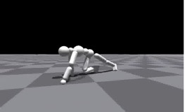
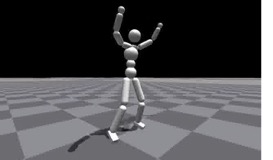
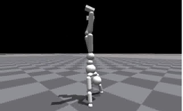
Figure 4: “Crawl”, “Jumping Jack”, “Skipping rope”, “Handstand”

We further examine the impact of robot mismatch. We vary the length of the humanoid robot’s single leg. Tab.2 illustrates that LAGOON is robust. Even when we reduce the leg length by 70%, the policy can execute backward runs and cartwheels. Note that the backward distance drops as the leg length is reduced by 40%. In this case, the humanoid robot jumps on a single leg, while still moving other limbs as if it is running.

Leg Difference	0	10%	20%	30%	40%	50%	60%	70%
Run Back Success (%)	98.8	99.7	99.0	96.6	97.6	91.0	94.8	96.3
Backward Distance	21.5	21.8	20.3	20.5	14.7	11.4	12.9	12.4
Cartwheel Success (%)	92.6	82.3	90.0	87.4	85.0	73.8	75.9	80.6
Cartwheel Direction	1.8	1.6	1.8	1.8	1.7	1.6	1.5	1.7

Table 2: We modify the humanoid robot’s single leg length. Here 0 indicates that the two legs have the same length.

5.2 Quadrupedal Robot

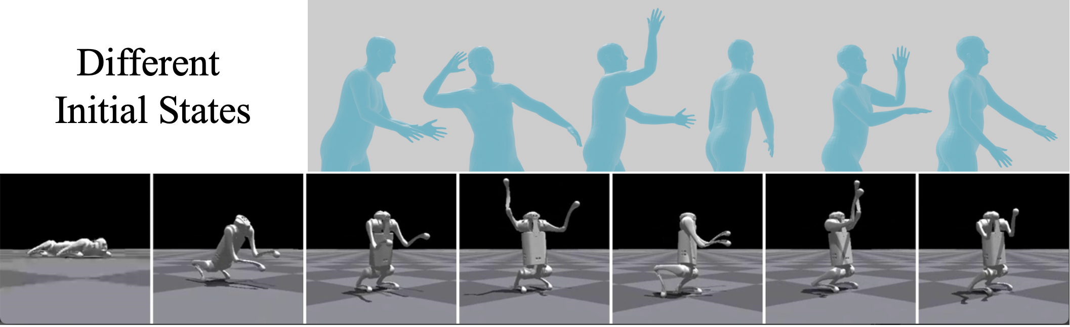
Figure 5: The task of “throw a ball” on the quadrupedal robot. Even though the getting up does not appear in the reference motion, the quadrupedal robot learns how to get up from the ground first and then wave its front legs.

It’s natural to transfer the generated motion when the embodiments are the same (i.e., human motion to humanoid robot). However, a significant skeletal disparity exists between humans and quadrupedal robots. The problem lies in how to retarget the motions. Our default strategy is to retarget the humans’ hands to the robots’ front legs and retarget the humans’ legs to the robots’ rear legs (more details in Appendix A.2).

we evaluate LAGOON on the task conditioned on the language text “the person throws a ball”. The quadrupedal robot has an essentially different body structure from the humans, and the initial states of the robots and the reference motion are largely different. The robot must first learn to “stand” like the humans without extra data. Since the root’s linear velocity and angular velocity could not be estimated precisely by the real-world go1 robot, we utilize the gravity projected on the robot’s up axis instead. The states of the quadrupedal robot policy include the projected gravity, the local velocity and rotation of each joint, and the actions taken in the last timestep. The training details are listed in Appendix.

The result in Fig. 5 demonstrates that LAGOON makes the policy “stand” on two feet first, then the robot successfully takes the behaviors “the person throws a ball”.

	Stand	Throw	Complete
LAGOON	✓	✓	✓
W/o Hybrid Initialization	✗	✓	✗
W/o Adversarial Reward	✗	✓	✗
W/o State-error Reward	✓	✗	✗
W/o Extra Critic Inputs	✓	✗	✗

Table 3: Abalation studies of LAGOON on a quadrupedal robot. Without hybrid initialization or adversarial reward, the robot can wave its front legs only if it initially stands on its rear legs. Without either the state-error reward or the augmented critic inputs, the robot is able to get up from the ground and stand on its rear legs but the doesn’t move its front legs afterward.

Abaltion study: We further conduct an ablation study on the quadrupedal robot, and the results are listed in Tab. 3. We split the complete task into two stages. “Stand” means the quadrupedal robot can get up from the ground. “Throw” means that the quadrupedal robot can wave the hand from the upright state. “Complete” means the robot can “stand” first and take the correct behaviors. We observe that the quadrupedal robot fails to stand without the adversarial reward. The state-error reward and the extra critic inputs make the policy learn fine-grained behavior.

Multiple retargeting strategy: We also demonstrate that there are multiple retargeting strategy options, and LAGOON works well for all of these strategies and generates diverse control policies. As depicted in Fig. 6, when provided with the language prompt ”walk backward,” we employ MDM to generate human motion. Subsequently, we retarget all the joints on the left side, causing the quadrupedal robot to walk backward using its two rear legs. We also replicate the states of the rear legs onto the front legs. Ultimately, the final policy enables the quadrupedal robot to walk on all four legs. In Fig.7, we utilize the motion of ”run backward” for the lower body retargeting, while the motion of ”raise arms” is applied to the upper body. This results in the quadrupedal robot running backward while simultaneously raising its front legs.

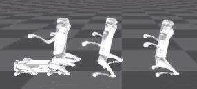
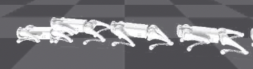
Figure 6: “Walk backward.” Left: Retarget all the joints. Right: Copy the rear joints’ states to the front joints when retargeting.

Figure 7: We retarget the motion of “run backward” to the lower body and retarget the motion of “raise arms” to the upper body.

5.3 Real-World Robot Deployment

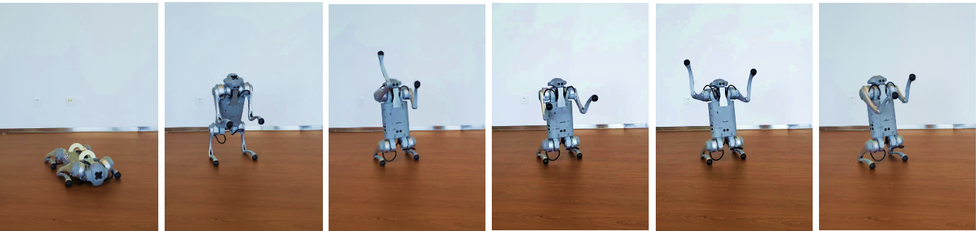
Figure 8: The real-world experiment on the quadrupedal robot. The language command is “the person throws a ball”. The robot stands up first and waves its front legs like throwing a ball.

There is a big dynamics gap between the simulator and the real world. For example, as shown in Fig. 5, the simulated robot stands on a single foot to mimic the reference motion. This behavior can be taken in the simulator but could harm the motor in the real world. Thus, in the experiment of the real-world robot, we only retarget the upper body of the generated motion to the two front legs of the robot when retargeting. The real-world results are demonstrated in Fig. 8. The quadrupedal robot produces behaviors consistent with the reference motion.

6 Conclusion

We propose a multi-phase method LAGOON to train robot control policy following the given language command. We first generate human motion using a language-conditioned motion diffusion model and create a semantically desired but physically unrealistic robot motion by retargeting the generated human motion to the robot skeleton. We adopt RL to train control policy and finally deploy the trained policy to the real world. LAGOON can also produce a robust policy that controls a real-world quadrupedal robot to stand up and take behaviors consistent with the language commands. We do admit there are limitations in specific modules. For example, the motion generation model (MDM) may produce errors itself. However, this can be improved with a better pre-trained model. Finally, many policies cannot be directly transferred to real robots due to hardware constraints. The issue of MDM and the sim2real gap are orthogonal to our LAGOON pipeline, and we are working on it as a future work for a robotics venue.

Appendix A Implementation Details

A.1 Motion Generation Details

We use the official implementation of Human Motion Generation Model [61] to generate motion sequences. They use the CLIP model to encode natural language descriptions and use a transformer denoiser over a 263-dimensional feature space proposed in [18]. The generated feature is then rendered into SMPL mesh [30]. In the sampling process, following their default hyper-parameters, we adopt the classifier-free guidance [21] with a guidance scale of $2.5$. We use cosine noise scheduling with 1000 diffusion steps.

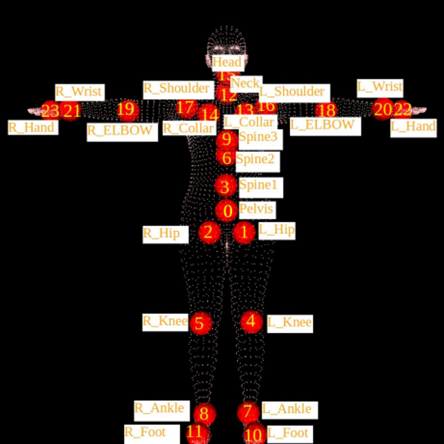
Figure 9: Skeleton layout of the SMPL [30] model. This image comes from the SMPL make simple tutorial (https://smpl-made-simple.is.tue.mpg.de/).

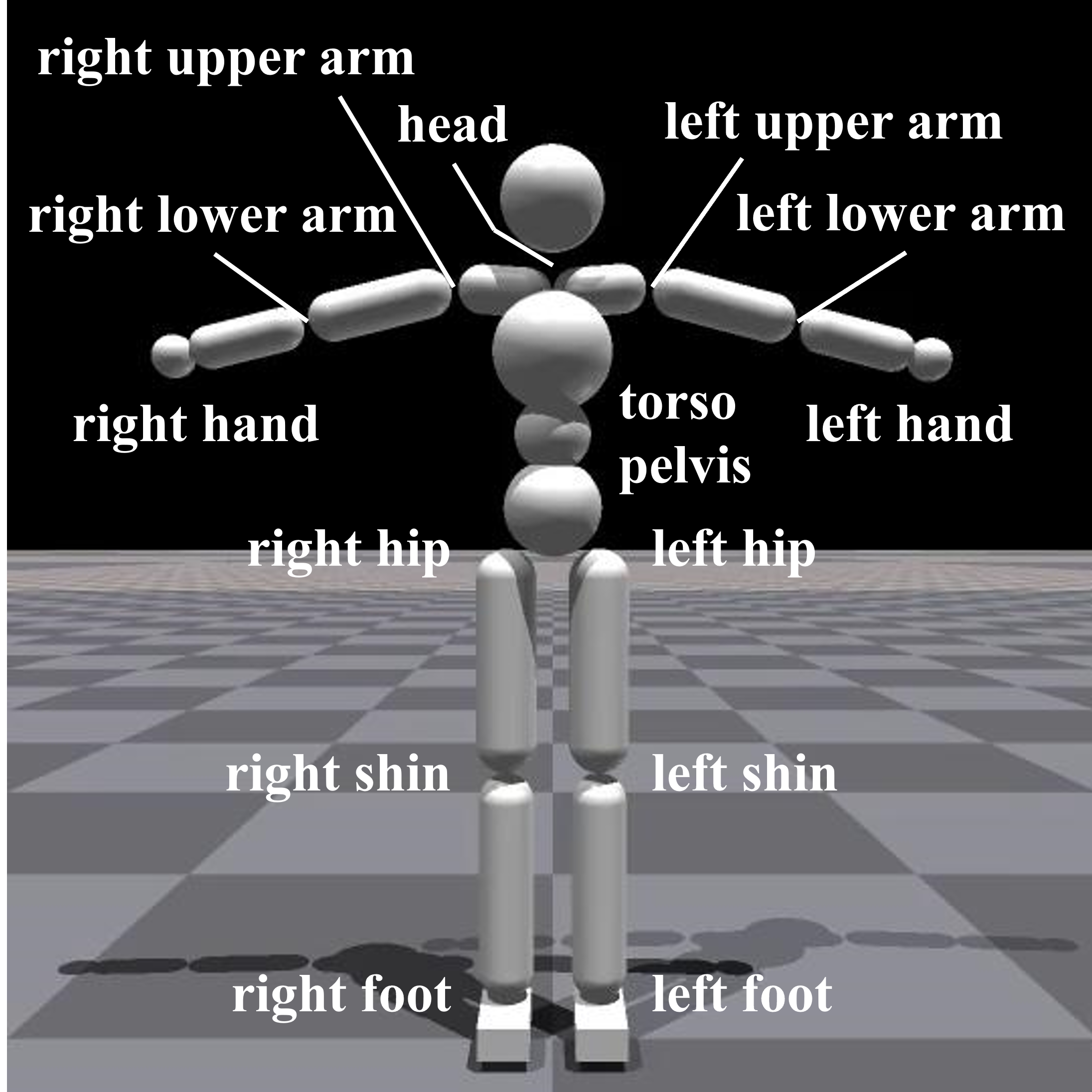
Figure 10: Skeleton layout of the humanoid robot.

A.2 Retargeting Details

We retarget the generated SMPL meshes to our target skeletons (humanoid or quadrupedal robot) using a script from Isaac Gym [33, 41]. First, we extract the root translation and local joint rotations from SMPL parameters. As presented in Fig. 10 and Fig. 10, the SMPL skeleton layout has more joints than our humanoid robot. We remove redundant joints and map the rest according to the mapping given in Tab. 4 and Tab. 5. Then we compute the relative joint rotations compared to a T-pose of the source motion. These rotations are applied on the target skeleton to obtain the retargeted motion.

For the humanoid robot, the elbows and knees (labeled “lower arm” and “shin” in Fig. 10) have only 1 DoF instead of 3 in the SMPL skeleton. We convert these 3D joints to 1D using inverse dynamics. Take the left arm as an example. We first compute the relative rotation angle between the left upper arm and the left lower arm and the local rotation of the left elbow is set to this angle. The local rotation of the left shoulder is then adjusted such that the position of the left hand stays in the original position.

The four legs of the quadrupedal robot have a similar structure. Take the right rear leg as an example. The hip, thigh, and calf (labeled 1, 4, and 7 in Fig. 11) have 1 DoF each. We apply different rules to retarget the arms and legs of an SMPL character to the front and rear legs of a quadrupedal robot. For the rear legs, the hips, knees, and ankles of the SMPL character are mapped to the hips, thighs, and calves of the quadrupedal robot, respectively. Redundant DoFs are discarded in this process. For the front legs, the elbow and wrist of the SMPL character are mapped to the calf and foot of the quadrupedal robot. The shoulder of the SMPL character has 3 DoFs. We map one of them to the front hip and one to the front thigh of the quadrupedal robot. The joint mappings are visualized in Fig. 11.

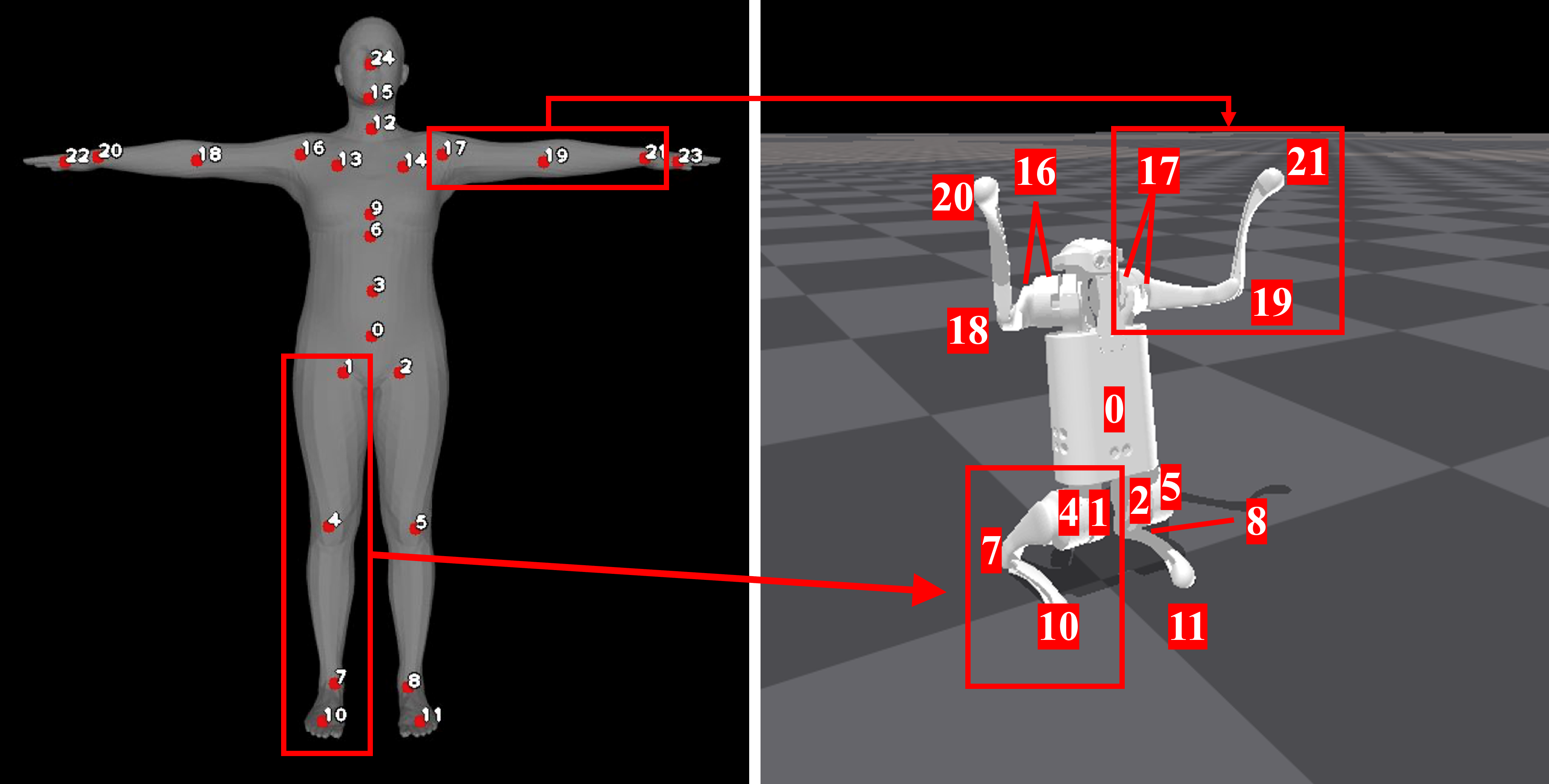
Figure 11: Joint mappings from the SMPL skeleton to the quadrupedal robot. Note that 16 and 17 in the quadrupedal skeleton each correspond to 2 joints. The joint names are listed in Tab. 5

Source Joints	Target Joints
Pelvis	pelvis
L_Hip	left_thigh
L_Knee	left_shin
L_Ankle	left_foot
R_Hip	right_thigh
R_Knee	right_shin
R_Ankle	right_foot
Spine3	torso
Neck	head
L_Shoulder	left_upper_arm
L_Elbow	left_lower_arm
L_Wrist	left_hand
R_Shoulder	right_upper_arm
R_Elbow	right_lower_arm
R_Wrist	right_hand

Table 4: Joint mapping between the SMPL skeleton (Source Joints) and the humanoid robot (Target Joints).

Source Joints	Target Joints	Joint Index
Pelvis	trunk	0
L_Hip	RL_hip	2
L_Knee	RL_thigh	5
L_Ankle	RL_calf	8
L_Foot	RL_foot	11
R_Hip	RR_hip	1
R_Knee	RR_thigh	4
R_Ankle	RR_calf	7
R_Foot	RR_foot	10
L_Shoulder	FL_hip, FL_thigh	17
L_Elbow	FL_calf	19
L_Wrist	FL_foot	21
R_Shoulder	FR_hip, FR_thigh	16
R_Elbow	FR_calf	18
R_Wrist	FR_foot	20

Table 5: Joint mapping between the SMPL skeleton (Source Joints) and the quadrupedal robot (Target Joints). “Target Joint Index” indicates the corresponding indicies in Fig. 11.

A.3 Training Details

A.3.1 Reinforcement Learning

We adopt Isaay Gym [33] as our physics simulator, as it enables massive parallel simulation on GPUs. For the humanoid robot, the simulation runs at 60Hz while the frequency of the control policy is 30Hz. The control policy $\pi_{\theta}$, the value function $V_{\phi}$, and the discriminator $D_{\psi}$ are MLPs with hidden dimensions (1024, 512) and ReLU activations. We adopt a fixed diagonal covariance matrix $\Sigma$ for the control policy, with all diagonal entries set to 0.05. We normalize the policy’s input state using a running estimate of the mean and variance of the states. We create 4096 parallel simulation environments in Isaac Gym to collect training samples. The max episode length of each simulation is 300. We update $\pi_{\theta}$, $V_{\phi}$, and $D_{\psi}$ 6 times every 16 steps of the environments, with a mini-batch size of 32768. The clipping coefficient of PPO is set to 0.2. The discount $\gamma$ of the MDP is set to 0.99. We also adopt GAE [51] to estimate the advantage of policy gradient and the GAE coefficient is set to 0.95. We adopt Adam [25] as the optimizer and set the learning rate as 5e-5. We train the policy for 5000 epochs. All the experiments on humanoid robots use the above hyper-parameters. For LAGOON, we set both $\lambda_{adv}$ and $\lambda_{err}$ to 1, except for the task “run backward” where $\lambda_{err}$ is set to $0.1$.

For the experiments on the quadrupedal robot, the simulation runs at 200Hz and the control policy runs at 50Hz. We run the experiments with 8192 environments for 20,000 epochs. The maximum episode length is set to 250. Other hyper-parameters are the same as the experiments on the humanoid robot.

We employ the technique of early termination [38, 41] to accelerate training. For the humanoid robot, we reset the environment when any joint of the humanoid, with the exception of feet, has a nonzero contact force. For the task “cartwheel”, the hands of the humanoid are also excluded. For the quadrupedal robot, an environment is reset if any joint rotation or angular velocity exceeds a certain limit. It is possible that the quadrupedal robot falls on the ground without triggering an early termination. We make sure that a quadrupedal robot in such a state receives a low reward on state similarity. The details about reward design will be described in Appendix. A.3.3.

A.3.2 States

For the humanoid robot, the state consists of:

• The root rotation, linear velocity, and angular velocity.

• Local rotations and angular velocities of each joint.

• Positions of the hands and feet.

For the quadrupedal robot, the root’s linear velocity and angular velocity could not be estimated precisely by the real-world go1 robot. Following [49], we utilize the gravity projected on the robot’s up axis and actions taken in the last timestep. The state consists of:

• Projected gravity.

• Local rotations and angular velocities of each joint.

• Positions of the hands and feet.

• Actions taken in the last timestep.

A.3.3 State Similarity

For the humanoid robot, we use the reward function in [38] as our state similarity metric:

$$\begin{split}Sim(y,s)&=0.65r_{p}+0.1r_{v}+0.15r_{e}+0.1r_{r}\\ r_{p}&=\exp\left[-2\sum_{j}(\|q_{s,j}-q_{y,j}\|^{2})\right]\\ r_{v}&=\exp\left[-0.1\sum_{j}(\|\dot{q}_{s,j}-\dot{q}_{y,j}\|^{2})\right]\\ r_{e}&=\exp\left[-40\sum_{e}(\|p_{s,e}-p_{y,e}\|^{2})\right]\\ r_{r}&=\exp\left[-10\|p_{s,r}-p_{y,r}\|^{2}\right]\end{split}$$ (5)

Here $q_{\cdot,j}$ and $\dot{q}_{\cdot,j}$ denote the local rotation and angular velocity of the $j$-th joint. $p_{\cdot,j}$ denotes the relative position to root of the $j$-th joint. We use relative positions to root instead of absolute positions since the humanoid robot may be initialized at random positions. $p_{\cdot,r}$ denotes the global root position.

For the quadrupedal robot, we additionally take into account the root rotation. Let $q_{\cdot,r}$ denote the root rotation. The similarity metric is changed to

$$Sim(y,s)=0.8r_{\mathrm{rot}}(0.65r_{p}+0.1r_{v}+0.15r_{e}+0.1r_{r})\\ +0.2r_{\mathrm{rot}},$$ (6)

where $r_{\mathrm{rot}}=\max(0,q_{s,r}\cdot q_{y,r})$. The $r_{\mathrm{rot}}$ term penalizes incorrect root rotations. Thus, when the quadrupedal robot falls over, it receives a low reward even if local rotations of other joints still match the reference motion.

A.3.4 State Matching

As dynamic programming can be time-consuming, we maintain a state matching $(u_{0:k},v_{0:k})$ and update it every certain number of epochs. The state matching is initialized as the simplest matching $u_{i}=v_{i}=i$. For the task “run back” and “kick”, the matching is updated every 4000 epochs. For the task “cartwheel”, the matching is updated every 1000 epochs. During each update, we collect 4096 episodes and use dynamic programming to compute a matching with the highest total reward for each episode. We filter out matched pairs of states with similarity less than $0.05$. Then we select the episode with the most states matched. As we will initialize the humanoid robot from two different states, we compute a matching for each state initialization.

Another effective matching for the task “run back” and “kick” is to simply match the initial states of the reference motion. More specifically, for a reference motion $y_{0:H}$ and a trajectory $s_{0:T}$ from the policy, we simply set $u_{i}=i$ and $v_{i}=i+t_{0}$, where $t_{0}=\min\{t\mid Sim(y_{0},s_{t})\geq 0.5\}$. This matching strategy is also effective for experiments on the quadrupedal robot.

A.4 Domain Randomization

For the humanoid robot, we use the default domain randomization parameters in Isaac Gym. We list the randomized physics parameters in Tab. 6. Except for observation, action, and rigid body mass, all the parameters are linearly interpolated between no randomization and max randomization in the first 3000 environment steps. Due to a current limitation of Isaac Gym, rigid body mass is randomized only once before the simulation is started. New randomizations are generated every 600 environment steps. We also randomize the terrain when training the humanoid robot. There are four terrains during training. “Plane” refers to a flat surface without variations in elevation. For the “Rand” terrain, we generate a height field where the height of a vertex is sampled from $\{0,0.2\text{m}\}$. The horizontal distance between two adjacent points is 0.5m. This height field is then converted into a triangle mesh. The “Pyramid” terrain is a square cone with steps. The step width is 0.5m and the step height is 0.05m. There is a flat platform at the peak of the pyramid with a side length of 1m. The “Wave” terrain is constructed from sine waves. More specifically, the height at $(x,y)$ is given by $0.5\cos(\pi x/6)+0.5\sin(\pi y/6)$ (in meters). Each terrain has a size of $240\text{m}\times 240\text{m}$. The humanoid robots are randomly initialized in the center $120\text{m}\times 120\text{m}$ region. This ensures that the robots do not leave the terrain within an episode.

Parameter	Operation	Distribution	Unit
Observation	Additive	$\mathcal{N}(0,0.002)$	-
Action	Additive	$\mathcal{N}(0,0.02)$	-
Gravity	Additive	$\mathcal{N}(0,0.4)$	$\mathrm{m}/\mathrm{s}^{2}$
Body Mass	Scaling	$\operatorname{U}(0.5,1.5)$	1
Body Friction	Scaling	$\operatorname{U}(0.7,1.3)$	1
Body Restitution	Scaling	$\operatorname{U}(0,0.7)$	1
Damping	Scaling	$\operatorname{U}(0.5,1.5)$	1
Stiffness	Scaling	$\operatorname{U}(0.5,1.5)$	1
Lower	Additive	$\mathcal{N}(0,0.01)$	$\mathrm{rad}$
Upper	Additive	$\mathcal{N}(0,0.01)$	$\mathrm{rad}$

Table 6: Randomization parameters of the humanoid robot. $U(a,b)$ denotes the uniform distribution over $[a,b]$. “Lower” and “Upper” refer to the lower bounds and upper bounds of the range of the DoFs.

For the quadrupedal robot, because of the limitation of Isaac Gym, we fix the ground friction coefficient and randomize the friction coefficients of the robot’s bodies. We train the policy on the plane terrain and set the friction and restitution coefficients of the ground as 0.6 and 0.4, respectively. We randomize the mass of the robot trunk and the friction of all the rigid bodies. We also randomize the proportional gain and derivative gain of the PD controller. In addition, we noise the observations. The detailed ranges are listed in Tab 7.

Parameter	Operation	Distribution	Unit
Obs.Gravity	Additive	$\operatorname{U}(-0.05,0.05)$	$\mathrm{m}/\mathrm{s}^{2}$
Obs.ROT	Additive	$\operatorname{U}(-0.01,0.01)$	$\mathrm{rad}$
Obs.VEL	Additive	$\operatorname{U}(-1.5,1.5)$	$\mathrm{rad}/\mathrm{s}$
Trunk Mass	Additive	$\operatorname{U}(0,1)$	$\mathrm{kg}$
Body Friction	Scaling	$\operatorname{U}(0.05,2)$	1
Proportional Gain	Scaling	$\operatorname{U}(0.7,1.3)$	1
Derivative Gain	Scaling	$\operatorname{U}(0.7,1.3)$	1

Table 7: Randomization parameters of the quadrupedal robot. $U(a,b)$ denotes the uniform distribution over $[a,b]$. We noise the policy inputs separately. Obs.Gravity refers to the projected gravity, Obs.ROT and Obs.VEL refers to the local rotations and velocities.

Appendix B Other Results on Quadrupedal Robot

In this section, we demonstrate more experiments on the quadrupedal robot. Please also refer to our videos.

B.1 Partial Retargeting

We conduct experiments on the quadrupedal robot by retargeting a subset of joints.

Turn around

We generate a motion sequence using the language prompt “turn around” and only retarget the root rotation. As presented in Fig. 12, the quadrupedal robot learns to turn around in the physics simulator.

It is important to note that we intended to show the flexibility and versatility of our approach by employing various retargeting strategies. We can also retarget all the bodies when mimicking the reference motion of “turning around.”(Fig.13), which makes the quadruped robot walk on its two rear legs and turn around.

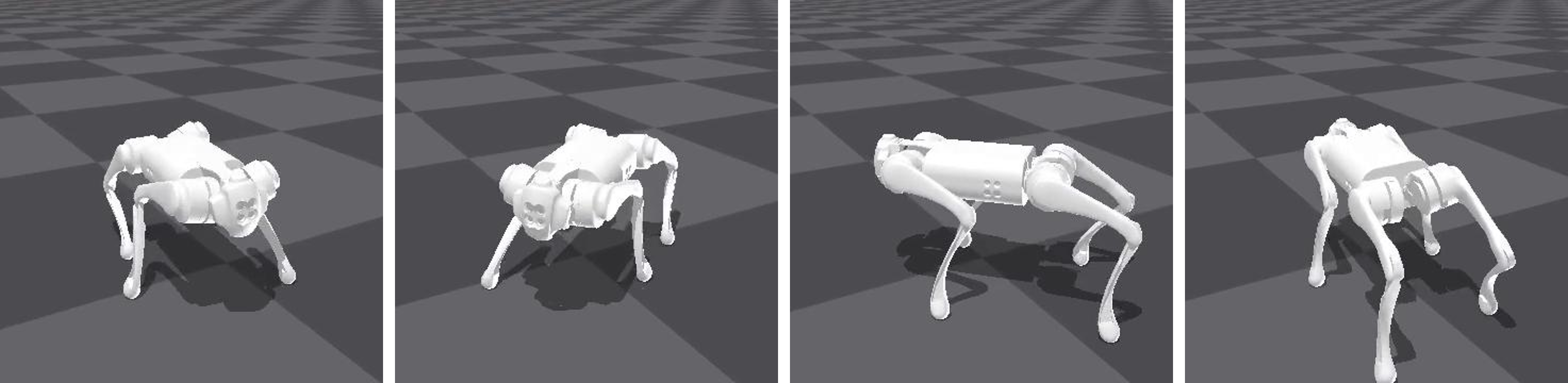
Figure 12: The quadrupedal robot is turning around. Note that only the root rotation is retargeted.

Figure 13: “Turn around”. We also retarget all the bodies when mimicking the reference motion of “turning around.” which makes the quadruped robot walk on its two rear legs and turn around.

Raise the left hand

We generate another motion sequence of a person raising the left hand by the language prompt “raise the left hand”. We retarget only the left arm to the left front leg of the quadrupedal robot. As shown in Fig. 14, the robot raises its left front leg with the other three legs on the ground in the reference motion. The learned policy can perform a similar behavior in the real world.

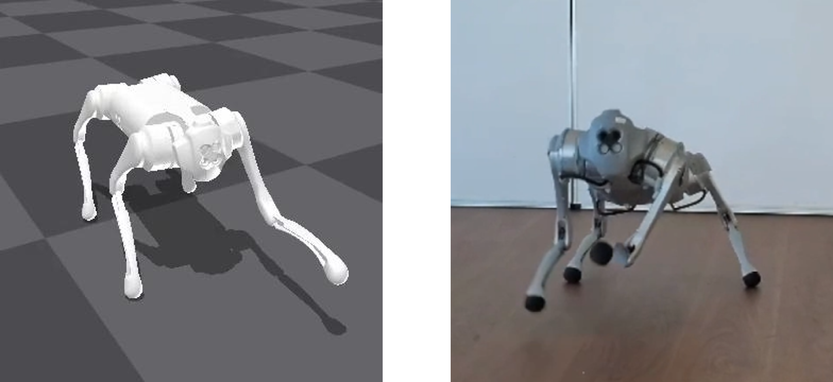
Figure 14: (Left) We only retarget the left arm of the SMPL character to the left front leg of the quadrupedal robot. (Right) The policy learns to raise the left front leg in the real world.

References

- [1] Michael Ahn, Anthony Brohan, Noah Brown, Yevgen Chebotar, Omar Cortes, Byron David, Chelsea Finn, Keerthana Gopalakrishnan, Karol Hausman, Alex Herzog, et al. Do as i can, not as i say: Grounding language in robotic affordances. arXiv preprint arXiv:2204.01691, 2022.
- [2] Chaitanya Ahuja and Louis-Philippe Morency. Language2pose: Natural language grounded pose forecasting. In 2019 International Conference on 3D Vision (3DV), pages 719–728. IEEE, 2019.
- [3] Anurag Ajay, Yilun Du, Abhi Gupta, Joshua Tenenbaum, Tommi Jaakkola, and Pulkit Agrawal. Is conditional generative modeling all you need for decision-making? arXiv preprint arXiv:2211.15657, 2022.
- [4] Mazen Al Borno, Martin de Lasa, and Aaron Hertzmann. Trajectory optimization for full-body movements with complex contacts. IEEE Transactions on Visualization and Computer Graphics, 19(8):1405–1414, 2013.
- [5] Jean-Baptiste Alayrac, Jeff Donahue, Pauline Luc, Antoine Miech, Iain Barr, Yana Hasson, Karel Lenc, Arthur Mensch, Katherine Millican, Malcolm Reynolds, Roman Ring, Eliza Rutherford, Serkan Cabi, Tengda Han, Zhitao Gong, Sina Samangooei, Marianne Monteiro, Jacob Menick, Sebastian Borgeaud, Andrew Brock, Aida Nematzadeh, Sahand Sharifzadeh, Mikolaj Binkowski, Ricardo Barreira, Oriol Vinyals, Andrew Zisserman, and Karen Simonyan. Flamingo: a visual language model for few-shot learning. In Alice H. Oh, Alekh Agarwal, Danielle Belgrave, and Kyunghyun Cho, editors, Advances in Neural Information Processing Systems, 2022.
- [6] Kevin Bergamin, Simon Clavet, Daniel Holden, and James Richard Forbes. DReCon: Data-driven responsive control of physics-based characters. ACM Trans. Graph., 38(6), nov 2019.
- [7] Uttaran Bhattacharya, Elizabeth Childs, Nicholas Rewkowski, and Dinesh Manocha. Speech2affectivegestures: Synthesizing co-speech gestures with generative adversarial affective expression learning. In Proceedings of the 29th ACM International Conference on Multimedia, pages 2027–2036, 2021.
- [8] Mariusz Bojarski, Davide Del Testa, Daniel Dworakowski, Bernhard Firner, Beat Flepp, Prasoon Goyal, Lawrence D Jackel, Mathew Monfort, Urs Muller, Jiakai Zhang, et al. End to end learning for self-driving cars. arXiv preprint arXiv:1604.07316, 2016.
- [9] Tom Brown, Benjamin Mann, Nick Ryder, Melanie Subbiah, Jared D Kaplan, Prafulla Dhariwal, Arvind Neelakantan, Pranav Shyam, Girish Sastry, Amanda Askell, Sandhini Agarwal, Ariel Herbert-Voss, Gretchen Krueger, Tom Henighan, Rewon Child, Aditya Ramesh, Daniel Ziegler, Jeffrey Wu, Clemens Winter, Chris Hesse, Mark Chen, Eric Sigler, Mateusz Litwin, Scott Gray, Benjamin Chess, Jack Clark, Christopher Berner, Sam McCandlish, Alec Radford, Ilya Sutskever, and Dario Amodei. Language models are few-shot learners. In H. Larochelle, M. Ranzato, R. Hadsell, M.F. Balcan, and H. Lin, editors, Advances in Neural Information Processing Systems, volume 33, pages 1877–1901. Curran Associates, Inc., 2020.
- [10] Tom Brown, Benjamin Mann, Nick Ryder, Melanie Subbiah, Jared D Kaplan, Prafulla Dhariwal, Arvind Neelakantan, Pranav Shyam, Girish Sastry, Amanda Askell, et al. Language models are few-shot learners. Advances in neural information processing systems, 33:1877–1901, 2020.
- [11] Mark Chen, Jerry Tworek, Heewoo Jun, Qiming Yuan, Henrique Ponde de Oliveira Pinto, Jared Kaplan, Harri Edwards, Yuri Burda, Nicholas Joseph, Greg Brockman, Alex Ray, Raul Puri, Gretchen Krueger, Michael Petrov, Heidy Khlaaf, Girish Sastry, Pamela Mishkin, Brooke Chan, Scott Gray, Nick Ryder, Mikhail Pavlov, Alethea Power, Lukasz Kaiser, Mohammad Bavarian, Clemens Winter, Philippe Tillet, Felipe Petroski Such, Dave Cummings, Matthias Plappert, Fotios Chantzis, Elizabeth Barnes, Ariel Herbert-Voss, William Hebgen Guss, Alex Nichol, Alex Paino, Nikolas Tezak, Jie Tang, Igor Babuschkin, Suchir Balaji, Shantanu Jain, William Saunders, Christopher Hesse, Andrew N. Carr, Jan Leike, Josh Achiam, Vedant Misra, Evan Morikawa, Alec Radford, Matthew Knight, Miles Brundage, Mira Murati, Katie Mayer, Peter Welinder, Bob McGrew, Dario Amodei, Sam McCandlish, Ilya Sutskever, and Wojciech Zaremba. Evaluating large language models trained on code, 2021.
- [12] Yilun Dai, Mengjiao Yang, Bo Dai, Hanjun Dai, Ofir Nachum, Josh Tenenbaum, Dale Schuurmans, and Pieter Abbeel. Learning universal policies via text-guided video generation. arXiv preprint arXiv:2302.00111, 2023.
- [13] Ashley Edwards, Himanshu Sahni, Yannick Schroecker, and Charles Isbell. Imitating latent policies from observation. In Kamalika Chaudhuri and Ruslan Salakhutdinov, editors, Proceedings of the 36th International Conference on Machine Learning, volume 97 of Proceedings of Machine Learning Research, pages 1755–1763. PMLR, 09–15 Jun 2019.
- [14] Alejandro Escontrela, Xue Bin Peng, Wenhao Yu, Tingnan Zhang, Atil Iscen, Ken Goldberg, and Pieter Abbeel. Adversarial motion priors make good substitutes for complex reward functions. 2022 IEEE/RSJ International Conference on Intelligent Robots and Systems (IROS), Oct 2022.
- [15] Tanmay Gangwani and Jian Peng. State-only imitation with transition dynamics mismatch. In International Conference on Learning Representations, 2020.
- [16] Anindita Ghosh, Noshaba Cheema, Cennet Oguz, Christian Theobalt, and Philipp Slusallek. Synthesis of compositional animations from textual descriptions. In Proceedings of the IEEE/CVF international conference on computer vision, pages 1396–1406, 2021.
- [17] Shiry Ginosar, Amir Bar, Gefen Kohavi, Caroline Chan, Andrew Owens, and Jitendra Malik. Learning individual styles of conversational gesture. In Proceedings of the IEEE/CVF Conference on Computer Vision and Pattern Recognition, pages 3497–3506, 2019.
- [18] Chuan Guo, Shihao Zou, Xinxin Zuo, Sen Wang, Wei Ji, Xingyu Li, and Li Cheng. Generating diverse and natural 3d human motions from text. In Proceedings of the IEEE/CVF Conference on Computer Vision and Pattern Recognition, pages 5152–5161, 2022.
- [19] Jonathan Ho and Stefano Ermon. Generative adversarial imitation learning. Advances in neural information processing systems, 29, 2016.
- [20] Jonathan Ho, Ajay Jain, and Pieter Abbeel. Denoising diffusion probabilistic models. Advances in Neural Information Processing Systems, 33:6840–6851, 2020.
- [21] Jonathan Ho and Tim Salimans. Classifier-free diffusion guidance. arXiv preprint arXiv:2207.12598, 2022.
- [22] Fangzhou Hong, Mingyuan Zhang, Liang Pan, Zhongang Cai, Lei Yang, and Ziwei Liu. AvatarCLIP: Zero-shot text-driven generation and animation of 3d avatars. ACM Trans. Graph., 41(4), jul 2022.
- [23] Mariko Isogawa, Ye Yuan, Matthew O’Toole, and Kris M Kitani. Optical non-line-of-sight physics-based 3d human pose estimation. In Proceedings of the IEEE/CVF Conference on Computer Vision and Pattern Recognition, pages 7013–7022, 2020.
- [24] Haresh Karnan, Faraz Torabi, Garrett Warnell, and Peter Stone. Adversarial imitation learning from video using a state observer. 2022 International Conference on Robotics and Automation (ICRA), May 2022.
- [25] Diederik P Kingma and Jimmy Ba. Adam: A method for stochastic optimization. arXiv preprint arXiv:1412.6980, 2014.
- [26] Hsin-Ying Lee, Xiaodong Yang, Ming-Yu Liu, Ting-Chun Wang, Yu-Ding Lu, Ming-Hsuan Yang, and Jan Kautz. Dancing to music. Advances in neural information processing systems, 32, 2019.
- [27] Jiaman Li, Yihang Yin, Hang Chu, Yi Zhou, Tingwu Wang, Sanja Fidler, and Hao Li. Learning to generate diverse dance motions with transformer. arXiv preprint arXiv:2008.08171, 2020.
- [28] Ruilong Li, Shan Yang, David A Ross, and Angjoo Kanazawa. Ai choreographer: Music conditioned 3d dance generation with aist++. In Proceedings of the IEEE/CVF International Conference on Computer Vision, pages 13401–13412, 2021.
- [29] Fangchen Liu, Zhan Ling, Tongzhou Mu, and Hao Su. State alignment-based imitation learning. In International Conference on Learning Representations, 2020.
- [30] Matthew Loper, Naureen Mahmood, Javier Romero, Gerard Pons-Moll, and Michael J Black. Smpl: A skinned multi-person linear model. ACM transactions on graphics (TOG), 34(6):1–16, 2015.
- [31] Zhengyi Luo, Ryo Hachiuma, Ye Yuan, and Kris Kitani. Dynamics-regulated kinematic policy for egocentric pose estimation. Advances in Neural Information Processing Systems, 34:25019–25032, 2021.
- [32] Zhengyi Luo, Shun Iwase, Ye Yuan, and Kris Kitani. Embodied scene-aware human pose estimation. arXiv preprint arXiv:2206.09106, 2022.
- [33] Viktor Makoviychuk, Lukasz Wawrzyniak, Yunrong Guo, Michelle Lu, Kier Storey, Miles Macklin, David Hoeller, Nikita Rudin, Arthur Allshire, Ankur Handa, and Gavriel State. Isaac gym: High performance gpu-based physics simulation for robot learning, 2021.
- [34] Gabriel B Margolis and Pulkit Agrawal. Walk these ways: Tuning robot control for generalization with multiplicity of behavior. Conference on Robot Learning, 2022.
- [35] Josh Merel, Yuval Tassa, Dhruva TB, Sriram Srinivasan, Jay Lemmon, Ziyu Wang, Greg Wayne, and Nicolas Heess. Learning human behaviors from motion capture by adversarial imitation, 2017.
- [36] Lars M. Mescheder, Andreas Geiger, and Sebastian Nowozin. Which training methods for gans do actually converge? In International Conference on Machine Learning, 2018.
- [37] Igor Mordatch, Emanuel Todorov, and Zoran Popović. Discovery of complex behaviors through contact-invariant optimization. ACM Trans. Graph., 31(4), jul 2012.
- [38] Xue Bin Peng, Pieter Abbeel, Sergey Levine, and Michiel van de Panne. DeepMimic: Example-guided deep reinforcement learning of physics-based character skills. ACM Trans. Graph., 37(4), jul 2018.
- [39] Xue Bin Peng, Marcin Andrychowicz, Wojciech Zaremba, and Pieter Abbeel. Sim-to-real transfer of robotic control with dynamics randomization. In 2018 IEEE international conference on robotics and automation (ICRA), pages 3803–3810. IEEE, 2018.
- [40] Xue Bin Peng, Erwin Coumans, Tingnan Zhang, Tsang-Wei Lee, Jie Tan, and Sergey Levine. Learning agile robotic locomotion skills by imitating animals. arXiv preprint arXiv:2004.00784, 2020.
- [41] Xue Bin Peng, Ze Ma, Pieter Abbeel, Sergey Levine, and Angjoo Kanazawa. AMP: Adversarial motion priors for stylized physics-based character control. ACM Trans. Graph., 40(4), jul 2021.
- [42] Mathis Petrovich, Michael J Black, and Gül Varol. Temos: Generating diverse human motions from textual descriptions. In Computer Vision–ECCV 2022: 17th European Conference, Tel Aviv, Israel, October 23–27, 2022, Proceedings, Part XXII, pages 480–497. Springer, 2022.
- [43] Alec Radford, Jong Wook Kim, Chris Hallacy, Aditya Ramesh, Gabriel Goh, Sandhini Agarwal, Girish Sastry, Amanda Askell, Pamela Mishkin, Jack Clark, et al. Learning transferable visual models from natural language supervision. In International conference on machine learning, pages 8748–8763. PMLR, 2021.
- [44] Aditya Ramesh, Prafulla Dhariwal, Alex Nichol, Casey Chu, and Mark Chen. Hierarchical text-conditional image generation with clip latents, 2022.
- [45] Aditya Ramesh, Mikhail Pavlov, Gabriel Goh, Scott Gray, Chelsea Voss, Alec Radford, Mark Chen, and Ilya Sutskever. Zero-shot text-to-image generation, 2021.
- [46] Davis Rempe, Leonidas J Guibas, Aaron Hertzmann, Bryan Russell, Ruben Villegas, and Jimei Yang. Contact and human dynamics from monocular video. In Computer Vision–ECCV 2020: 16th European Conference, Glasgow, UK, August 23–28, 2020, Proceedings, Part V 16, pages 71–87. Springer, 2020.
- [47] Zhiyuan Ren, Zhihong Pan, Xin Zhou, and Le Kang. Diffusion motion: Generate text-guided 3d human motion by diffusion model. arXiv preprint arXiv:2210.12315, 2022.
- [48] Robin Rombach, Andreas Blattmann, Dominik Lorenz, Patrick Esser, and Bjorn Ommer. High-resolution image synthesis with latent diffusion models. 2022 IEEE/CVF Conference on Computer Vision and Pattern Recognition (CVPR), Jun 2022.
- [49] Nikita Rudin, David Hoeller, Philipp Reist, and Marco Hutter. Learning to walk in minutes using massively parallel deep reinforcement learning. In Conference on Robot Learning, pages 91–100. PMLR, 2022.
- [50] Karl Schmeckpeper, Oleh Rybkin, Kostas Daniilidis, Sergey Levine, and Chelsea Finn. Reinforcement learning with videos: Combining offline observations with interaction. In Jens Kober, Fabio Ramos, and Claire Tomlin, editors, Proceedings of the 2020 Conference on Robot Learning, volume 155 of Proceedings of Machine Learning Research, pages 339–354. PMLR, 16–18 Nov 2021.
- [51] John Schulman, Philipp Moritz, Sergey Levine, Michael Jordan, and Pieter Abbeel. High-dimensional continuous control using generalized advantage estimation. arXiv preprint arXiv:1506.02438, 2015.
- [52] John Schulman, Filip Wolski, Prafulla Dhariwal, Alec Radford, and Oleg Klimov. Proximal policy optimization algorithms. CoRR, abs/1707.06347, 2017.
- [53] Younggyo Seo, Kimin Lee, Stephen L James, and Pieter Abbeel. Reinforcement learning with action-free pre-training from videos. In Kamalika Chaudhuri, Stefanie Jegelka, Le Song, Csaba Szepesvari, Gang Niu, and Sivan Sabato, editors, Proceedings of the 39th International Conference on Machine Learning, volume 162 of Proceedings of Machine Learning Research, pages 19561–19579. PMLR, 17–23 Jul 2022.
- [54] Pierre Sermanet, Corey Lynch, Yevgen Chebotar, Jasmine Hsu, Eric Jang, Stefan Schaal, Sergey Levine, and Google Brain. Time-contrastive networks: Self-supervised learning from video. 2018 IEEE International Conference on Robotics and Automation (ICRA), May 2018.
- [55] Rotem Shalev-Arkushin, Amit Moryossef, and Ohad Fried. Ham2Pose: Animating sign language notation into pose sequences. arXiv preprint arXiv:2211.13613, 2022.
- [56] Soshi Shimada, Vladislav Golyanik, Weipeng Xu, and Christian Theobalt. Physcap: Physically plausible monocular 3d motion capture in real time. ACM Transactions on Graphics (ToG), 39(6):1–16, 2020.
- [57] Mohit Shridhar, Lucas Manuelli, and Dieter Fox. Cliport: What and where pathways for robotic manipulation. In Conference on Robot Learning, pages 894–906. PMLR, 2022.
- [58] Uriel Singer, Adam Polyak, Thomas Hayes, Xi Yin, Jie An, Songyang Zhang, Qiyuan Hu, Harry Yang, Oron Ashual, Oran Gafni, Devi Parikh, Sonal Gupta, and Yaniv Taigman. Make-A-Video: Text-to-video generation without text-video data. In The Eleventh International Conference on Learning Representations, 2023.
- [59] Jascha Sohl-Dickstein, Eric Weiss, Niru Maheswaranathan, and Surya Ganguli. Deep unsupervised learning using nonequilibrium thermodynamics. In International Conference on Machine Learning, pages 2256–2265. PMLR, 2015.
- [60] Jiaming Song, Chenlin Meng, and Stefano Ermon. Denoising diffusion implicit models. arXiv preprint arXiv:2010.02502, 2020.
- [61] Guy Tevet, Sigal Raab, Brian Gordon, Yonatan Shafir, Daniel Cohen-Or, and Amit H Bermano. Human motion diffusion model. arXiv preprint arXiv:2209.14916, 2022.
- [62] Faraz Torabi, Garrett Warnell, and Peter Stone. Behavioral cloning from observation. Proceedings of the Twenty-Seventh International Joint Conference on Artificial Intelligence, Jul 2018.
- [63] Faraz Torabi, Garrett Warnell, and Peter Stone. Generative adversarial imitation from observation, 2018.
- [64] Jonathan Tseng, Rodrigo Castellon, and C. Karen Liu. EDGE: Editable dance generation from music, 2022.
- [65] Luca Viano, Yu-Ting Huang, Parameswaran Kamalaruban, Craig Innes, Subramanian Ramamoorthy, and Adrian Weller. Robust learning from observation with model misspecification. In Proceedings of the 21st International Conference on Autonomous Agents and Multiagent Systems, AAMAS ’22, page 1337–1345, Richland, SC, 2022. International Foundation for Autonomous Agents and Multiagent Systems.
- [66] Shusheng Xu, Huaijie Wang, and Yi Wu. Grounded reinforcement learning: Learning to win the game under human commands. In Alice H. Oh, Alekh Agarwal, Danielle Belgrave, and Kyunghyun Cho, editors, Advances in Neural Information Processing Systems, 2022.
- [67] Sijie Yan, Zhizhong Li, Yuanjun Xiong, Huahan Yan, and Dahua Lin. Convolutional sequence generation for skeleton-based action synthesis. In Proceedings of the IEEE/CVF International Conference on Computer Vision, pages 4394–4402, 2019.
- [68] Xinyu Yi, Yuxiao Zhou, Marc Habermann, Soshi Shimada, Vladislav Golyanik, Christian Theobalt, and Feng Xu. Physical inertial poser (pip): Physics-aware real-time human motion tracking from sparse inertial sensors. In Proceedings of the IEEE/CVF Conference on Computer Vision and Pattern Recognition, pages 13167–13178, 2022.
- [69] Chao Yu, Akash Velu, Eugene Vinitsky, Yu Wang, Alexandre Bayen, and Yi Wu. The surprising effectiveness of ppo in cooperative, multi-agent games. arXiv preprint arXiv:2103.01955, 2021.
- [70] Wenhao Yu, Greg Turk, and C. Karen Liu. Learning symmetric and low-energy locomotion. ACM Transactions on Graphics, 37(4):1–12, Jul 2018.
- [71] Ye Yuan and Kris Kitani. 3d ego-pose estimation via imitation learning. In Proceedings of the European Conference on Computer Vision (ECCV), pages 735–750, 2018.
- [72] Ye Yuan and Kris Kitani. Ego-pose estimation and forecasting as real-time pd control. In Proceedings of the IEEE/CVF International Conference on Computer Vision, pages 10082–10092, 2019.
- [73] Ye Yuan and Kris Kitani. Residual force control for agile human behavior imitation and extended motion synthesis. Advances in Neural Information Processing Systems, 33:21763–21774, 2020.
- [74] Ye Yuan, Jiaming Song, Umar Iqbal, Arash Vahdat, and Jan Kautz. Physdiff: Physics-guided human motion diffusion model. arXiv preprint arXiv:2212.02500, 2022.
- [75] Ye Yuan, Shih-En Wei, Tomas Simon, Kris Kitani, and Jason Saragih. Simpoe: Simulated character control for 3d human pose estimation. In Proceedings of the IEEE/CVF conference on computer vision and pattern recognition, pages 7159–7169, 2021.
- [76] Kevin Zakka, Andy Zeng, Pete Florence, Jonathan Tompson, Jeannette Bohg, and Debidatta Dwibedi. XIRL: Cross-embodiment inverse reinforcement learning. In 5th Annual Conference on Robot Learning, 2021.
- [77] Mingyuan Zhang, Zhongang Cai, Liang Pan, Fangzhou Hong, Xinying Guo, Lei Yang, and Ziwei Liu. Motiondiffuse: Text-driven human motion generation with diffusion model. arXiv preprint arXiv:2208.15001, 2022.
- [78] Kaifeng Zhao, Shaofei Wang, Yan Zhang, Thabo Beeler, and Siyu Tang. Compositional human-scene interaction synthesis with semantic control. In Computer Vision – ECCV 2022: 17th European Conference, Tel Aviv, Israel, October 23–27, 2022, Proceedings, Part VI, page 311–327, Berlin, Heidelberg, 2022. Springer-Verlag.
- [79] Rui Zhao, Hui Su, and Qiang Ji. Bayesian adversarial human motion synthesis. In Proceedings of the IEEE/CVF Conference on Computer Vision and Pattern Recognition, pages 6225–6234, 2020.