Infinite horizon optimal control of a SIR epidemic
under an ICU constraint

Abstract

The aim of this paper is to provide a rigorous mathematical analysis of an optimal control problem of a SIR epidemic on an infinite horizon. A state constraint related to intensive care units (ICU) capacity is imposed and the objective functional linearly depends on the state and the control. After preliminary asymptotic and viability analyses, a $\Gamma$-convergence argument is developed to reduce the problem to a finite horizon allowing to use a state constrained version of Pontryagin’s theorem to characterize the structure of the optimal controls. Illustrating examples and numerical simulations are given according to the available data on Covid-19 epidemic in Italy.

Keywords: Optimal control; SIR; $\Gamma$-convergence; Pontryagin principle; State constraints; Viability; Epidemics; Infinite horizon.

1 Introduction

The optimal control of epidemics ([2, 5, 25, 32]) have attracted the interest of researchers since the introduction of the first compartmental epidemic model by Kermack and McKendrick [28]. Lots of new contributions have appeared in recent years, particularly after the start of the COVID-19 pandemic – see for example  [1, 21, 20, 29, 30]. In this paper, we focus on the optimal control of the SIR model [28]

$$\begin{cases}\dfrac{ds}{dt}(t)=-\big{(}\beta-u(t)\big{)}\,s(t)\,i(t)\\[8.61108pt] \dfrac{di}{dt}(t)=\big{(}\beta-u(t)\big{)}\,s(t)\,i(t)-\gamma i(t)\\[8.61108pt] s(0)=s_{0},\ i(0)=i_{0}\end{cases}\qquad,\,t\in I,$$ (1.1)

with $\beta>0$, on an infinite time horizon $I=(0,\infty)$. The unknowns $s$ and $i$ in the system (1.1) represent the density functions of the susceptible and infectious populations, respectively. The total population is assumed to be constant and the third recovered class $r$ of SIR is classically obtained by using the conservation of mass. In Section 2 we recall some other epidemiological concepts related with the SIR model, like, for instance, the herd immunity threshold and the basic reproduction number $R_{0}$. Under a prescribed threshold $i_{M}\in(0,1)$, the initial conditions are taken to be $i_{0}\in(0,i_{M}]$ and $s_{0}\in(0,1-i_{0}]$. The problem is studied under the control constraints $u\in U:=L^{\infty}(I;[0,u_{\max}])$ with $0<u_{\max}<\beta$ and the state constraint

$$i(t)\leq i_{M},\ \forall\,t\in I.$$

Here, $u_{\max}$ represents the maximal realistic control effort that can be done to avoid the epidemic spread. Also $i_{M}$ is prescribed and it represents an intensive care unit (ICU) safety upper bound to the capacity of the health-care system to treat infected patients.

In our problem, $u(t)$ plays the role of a control variable that, typically, models any kind of non-pharmaceutical intervention suitable for reducing the transmission rate $\beta$. The derivatives in (1.1) are meant in a distibutional sense and the trajectories are constructed from admissible controls $u\in U$.

The optimal control problem that we aim to consider here is to minimize on the whole time horizon a linear integral cost functional depending both on the state $i$ and on the control $u$, that is

$$J^{\infty}(u,s,i)=\int_{I}\big{(}\lambda_{1}u+\lambda_{2}i\big{)}\,dt$$ (1.2)

where $(s,i)$ is the epidemic trajectory (i.e. solution of (1.1)) corresponding to the control $u$. The cost functional $J^{\infty}$ represents the cost of treatments and hospitalization for the populations $i$ of infected individuals and its dependence on $u$ allows to capture the economic and social cost of non-pharmaceutical interventions like slowdown, isolation, quarantine and distance measures in general.

For a cost functional depending only on the control (that is for $\lambda_{2}=0$) this problem has been considered in Miclo [33]. When $I$ is a bounded interval, that is for a finite time horizon, it has been studied in [4]. To be more precise, in [4] we have considered a finite horizon, state-independent, cost which corresponds to the choice $\lambda_{2}=0$. A viability study developed there is useful also in the present paper. In particular, we characterized a maximal zone ${\mathcal{A}}$ in which no control is needed to keep the infections under the level $i_{M}$, and a larger zone ${\mathcal{B}}$ in which policies allowing the trajectory to satisfy the constraints exist. Using these characterizations, we established the optimality of the greedy strategy acting only when the trajectory is about to exit the viable set. In particular, it is optimal to stop any control policy as soon as the immunity threshold $s=\frac{\gamma}{\beta}$ is reached. As a consequence, any optimal control for $I=(0,+\infty)$ is optimal also for a finite horizon problem $(0,T)$ with $T$ large enough.

The greedy policy, which is optimal for the state independent cost considered in [4], can no longer be expected to be optimal when the cost (1.2) also depends on $i$, or, at least when the contribution of the term involving the state is able to influence the control policy, that is if $\lambda_{2}$ is big enough. Moreover, differently from the control, the state function $i$ vanishes only as $t\to\infty$ and the reduction to a finite horizon argument used before does not work and must be refined. In particular, it will be shown that, in this case as well, a reduction to finite horizon problems can be obtained, albeit this is done by a $\Gamma$-convergence argument.

The variational property of $\Gamma$-convergence implies that, if $u^{T}$ is an optimal control (which can be shown to exist) for the problem with finite horizon $T$ (extended by $0$ to the whole infinite horizon) then, as $T$ goes to $\infty$ and up to a subsequence, $u^{T}$ converges to $u$ weakly* in $L^{\infty}$, and $u$ is optimal on the infinite horizon.

Since $u$ is optimal, then it is easy to see that herd immunity must be reached in a finite time (see Corollary 6.3). As a consequence, for any $T$ large enough, the susceptible population corresponding to the optimal control $u^{T}$ satisfies $s(T)<\frac{\gamma}{\beta}$. We are, then, led to characterize the optimal controls for such $T$ large enough being allowed, in doing it, to use the final condition $s(T)<\frac{\gamma}{\beta}$ as a necessary optimality condition (not as an assumption). This property of the approximating optimal controls on a finite horizon has a very important simplifying consequence in the application of Pontryagin’s principle, because it implies normality (see the proof of Theorem 9.1 and 9.7). For this reason, for this specific problem, considering an infinite horizon is more effective than working on a finite one. Pontryagin’s principle, in a version suitable to take into account state contraints, allows to characterize the controls $u^{T}$ and, hence, the control $u$ by taking the weak* limit as $T$ goes to $\infty$.

The paper is organized as follows. In Section 2 we state existence, uniqueness and asymptotic behavior of solutions of the controlled SIR system. In particular, it is shown that if the control has a finite integral on the infinite horizon, then the herd immunity must be reached in finite time. In Section 3 we revisit a viability analysis already done in [4] by using only elementary methods. This analysis is also useful to enlighten the “laminar flow argument” that will be used also in the subsequent sections. In Section 4 we introduce the greedy control strategy and show examples of the viability zones compatible with two different times of the Covid-19 epidemic in Italy. In Section 5 we formulate the infinite horizon optimal control problem with a general cost and prove the existence of a solution. The case of a linear cost is treated in the subsequent Section 6. Section 7 is devoted to reduction by $\Gamma$-convergence to a finite horizon problem. In Section 8 we use a version of Pontryagin’s theorem, suitable for state constrained problems, to derive necessary conditions of optimality for a finite horizon sufficiently large. In Section 9 we characterize the structure of the optimal controls on the finite as well as on the infinite horizon. To numerically illustrate our results we choose the framework of Covid-19 epidemic in Italy and perform some simulations in Section 10 by using the solver Bocop, [37, 7].

Notation. Along the paper, we denote by

• $U:=L^{\infty}(I;K)$ the space of (equivalence classes of) Lebesgue measurable and essentially bounded functions defined on $I$ and taking values in the compact set $K:=[0,u_{\max}]$;

• $Y:=W^{1,\infty}(I;\mathbb{R}^{2})$ the Sobolev space of (equivalence classes of) functions that are essentially bounded together with their distributional derivative defined on $I$ and taking values in $\mathbb{R}^{2}$; it is well known that every function in this space has a Lipschitz continuous representative.

2 Analysis of the controlled system

We refer to the Cauchy problem (1.1) as being the controlled system, because the control function $u$ appears as an input in the state differential equations. The uncontrolled one corresponds to the case in which $u$ is identically equal to $0$. This section is devoted to study existence, uniqueness and asymptotic behavior of the solutions of the aforementioned controlled system. From the point of view of mathematical analysis, the controlled case differs from the uncontrolled one. The uncontrolled system has constant coefficients and this makes it quite easy to study and the solution is continuously differentiable. On the contrary, the controlled system has variable and possibly discontinuous coefficients. Then, $C^{1}$ solutions are no longer expected and their asymptotic behavior is harder to study (see also [33]).

Theorem 2.1

For every control $u\in U$ and every initial condition $i_{0}\in(0,1)$ and $s_{0}\in(0,1-i_{0}]$ the controlled system (1.1) admits a unique solution $(s,i)\in Y$. Moreover, $(s(t),i(t))\in\mathbb{T}:=\{(s,i)\in(0,1]^{2}\ :\ s+i\leq 1\}$ for every $t\in I$.

Let us remark that, in particular, the population densities $s$ and $i$ are always strictly positive and belong to the invariant triangle $\mathbb{T}$. A crucial role in the proof is played by the observation that the sum of the two equations gives

$$(s+i)^{\prime}=-\gamma i.$$ (2.1)

Since $i$ is positive, this implies that $s+i$ is decreasing.

Proof. Since the dynamic is locally Lipschitz, then it is classical that we have local existence and uniqueness of an absolutely continuous solution (see for instance [24, I.3]). Let us denote by $J$, with $0\in J$, a time interval in which the unique solution $(s,i)$ exists.

Let us claim that $s(t)>0$ and $i(t)>0$ for every $t\in J$. Indeed, considering $i$ as a coefficient, the function $s$ is the unique solution of the linear Cauchy problem

$$\begin{cases}s^{\prime}=-(\beta-u)si\\ s(0)=s_{0}>0,\end{cases}$$

which is given by

$$s(t)=s_{0}{\mathop{\rm e}\nolimits}^{-\int_{0}^{t}(\beta-u(\xi))i(\xi)\,d\xi}\quad\forall\,t\in J.$$

Hence $s$ is strictly positive in $J$. Similarly, one can prove that also $i$ is strictly positive.

Since, as already remarked, $s+i$ is decreasing, we have

$$0<s(t)+i(t)\leq s_{0}+i_{0}\quad\forall\,t\in J,$$

and hence

$$(s(t),i(t))\in\mathbb{T}:=\{(s,i)\in(0,1]^{2}\ :\ s+i\leq 1\}$$

for every $t\in J$. Being bounded, the solution exists for every $t\in[0,+\infty)$.

Finally, looking at the equations, one sees that $s$ and $i$ have bounded derivatives, hence they are Lipschitz continuous and the theorem is completely proven. $\square$

Remark 2.2 (Notation)

Whenever the control $u$ and the initial conditions $s(0)=s_{0},\ i(0)=i_{0}$ are fixed, the unique solution to (1.1) will also be denoted by $(s^{s_{0},i_{0},u},i^{s_{0},i_{0},u})$. However, in the sequel, when the initial conditions are fixed or can be easily deduced from the context, we write simply $(s^{u},i^{u})$, or even $(s,i)$ if also the control is fixed or easy to deduce. This notation will be used throughout the whole paper.

In addition to the notation just introduced, for the rest of this section, we enforce the assumptions of Theorem 2.1, that is,

$$i_{0}\in(0,1),\ s_{0}\in(0,1-i_{0}],\ u\in U.$$

Lemma 2.3

The solutions $s$ and $i$ are related by the following integro-differential equation

$$s(t)+i(t)-s_{0}-i_{0}={\gamma}\int_{0}^{t}\frac{s^{\prime}(\tau)}{(\beta-u(\tau))s(\tau)}\,d\tau$$ (2.2)

for every $t\in I$.

Proof. By integrating (2.1) between $0$ and $t$ we have

$$s(t)+i(t)-s_{0}-i_{0}=-\gamma\int_{0}^{t}i(\tau)\,d\tau.$$ (2.3)

Equation (2.2) is then obtained by using the first state equation to substitute $i$ in the integral.

$\square$

The next theorem deals with the asymptotic behavior of the epidemic trajectory.

Proposition 2.4

The following propositions hold:

1. $s$ is strictly decreasing;

2. $\displaystyle s_{\infty}:=\lim_{t\to+\infty}s(t)\in(0,1)$ and $\displaystyle i_{\infty}:=\lim_{t\to+\infty}i(t)=0$;

3. $s_{\infty}<\frac{\gamma}{\beta-u_{\max}}$.

Proof. 1. By the first equation and the strict positivity of $s$ and $i$ we have $s^{\prime}<0$ in $I$; hence the claimed monotonicity.

2. By monotonicity and positivity, the limit $s_{\infty}:=\lim_{t\to+\infty}s(t)$ exists and is finite. Since $s+i$ is decreasing (see (2.1)) and positive, then $\lim_{t\to+\infty}\big{(}s(t)+i(t)\big{)}$ exists and is finite. As a consequence, also the limit

$$i_{\infty}:=\lim_{t\to+\infty}i(t)=\lim_{t\to+\infty}\big{(}s(t)+i(t)-s(t)\big{)}=\lim_{t\to+\infty}\big{(}s(t)+i(t)\big{)}-s_{\infty}$$

exists and is finite.

Let us consider now Lemma 2.3. Since $\frac{1}{\beta}\leq\frac{1}{\beta-u(\tau)}$ and $\frac{s^{\prime}(\tau)}{s(\tau)}<0$, by using (2.2) we have

$$s(t)+i(t)-s_{0}-i_{0}\leq\frac{\gamma}{\beta}\int_{0}^{t}\frac{s^{\prime}(\tau)}{s(\tau)}\,d\tau=\frac{\gamma}{\beta}\log\frac{s(t)}{s_{0}}.$$

Taking the limit as $t\to\infty$ then we get

$$s_{\infty}+i_{\infty}-s_{0}-i_{0}\leq\frac{\gamma}{\beta}\log\frac{s_{\infty}}{s_{0}},$$

with the convention that $\log 0:=-\infty$. Since $s$ is positive, we have $s_{\infty}\geq 0$. On the other hand, if we had $s_{\infty}=0$, by the previous inequality, we would get $i_{\infty}-s_{0}-i_{0}\leq-\infty$, which is clearly impossible. Hence, $s_{\infty}>0$.

It remains to prove that $i_{\infty}=0$. Of course, we have $i_{\infty}\geq 0$. Assume by contradiction that $i_{\infty}>0$. Then, there exists $\bar{t}>0$ such that $i(t)>{i_{\infty}}/{2}$ for all $t\geq\bar{t}$. By the first state equation, and since $s(t)\geq s_{\infty}>0$ and $\beta-u(t)\geq\beta-u_{\max}$, we would have

$$s^{\prime}(t)\leq-(\beta-u_{\max})s_{\infty}\frac{i_{\infty}}{2}<0,\quad\forall\,t\geq\bar{t},$$

leading to the contradiction $s_{\infty}=-\infty$.

3. Since $s$ is decreasing, if $s_{0}\leq\gamma/(\beta-u_{\max})$, then there is nothing to prove. Let us then assume that $s_{0}>\frac{\gamma}{\beta-u_{\max}}$. Let us denote by

$$t_{\max}:=\sup\{t\in[0,+\infty)\ :\ s(t)>\dfrac{\gamma}{\beta-u_{\max}}\}$$

and assume, by contradiction, that $t_{\max}=\infty$. Since $u\leq u_{\max}$, we have

$$i^{\prime}(t)=\big{(}(\beta-u(t))s(t)-\gamma\big{)}i(t)\geq\big{(}(\beta-u_{\max})s(t)-\gamma\big{)}i(t)>0\quad\forall\,t>0,$$

hence $i$ is increasing. Then, for every $t\in[0,+\infty)$ we have

$$s^{\prime}(t)=-(\beta-u(t))s(t)i(t)\leq-(\beta-u_{\max})s(t)i(t)\leq-\gamma i(t)\leq-\gamma i_{0}.$$

By integrating on $[0,t)$, we would have

$$s(t)\leq s_{0}-\gamma i_{0}t,\quad\forall\,t\geq 0,$$

and therefore $\lim_{t\to+\infty}s(t)=-\infty$, which contradicts 2.

It follows that $t_{\max}<\infty$. Then, by continuity, $s(t_{\max})=\frac{\gamma}{\beta-u_{\max}}$ and the claim follows by the strict monotonicity of $s$.

$\square$

By the second equation of the uncontrolled SIR system (1.1) (with $u=0$), since $i$ is positive, we deduce that

$$i^{\prime}(t)\leq 0\ \iff\ s(t)\leq\frac{\gamma}{\beta}.$$

The number $\frac{\gamma}{\beta}$ is the herd immunity threshold. Since $s$ is decreasing, when immunity is reached, $i$ starts to decrease and continues to do it for every time after. In the SIR model, the immunity threshold is the reciprocal of the basic reproduction number $R_{0}$ (see, for instance, [26]).

Remark 2.5

In Proposition 2.4 we have proved that $s_{\infty}<\frac{\gamma}{\beta-u_{\max}}$. This number is strictly greater than $\frac{\gamma}{\beta}$. If $u\equiv 0$, then we have $s_{\infty}<\frac{\gamma}{\beta}$, by simply taking $u_{\max}=0$ in point 3. of Proposition 2.4. On the other hand, it is easy to see that the herd immunity may not be reached if the control $u$ is big enough. That is, it may happen that $s_{\infty}>\frac{\gamma}{\beta}$.

The next theorem provides a very useful sufficient condition that ensures that herd immunity is reached in finite time. Proposition 2.4 is quite standard, even if not trivial for the controlled system. On the contrary, to the best of our knowledge, Theorem 2.6 is new. It plays an important role in the optimal control problems that will be considered in the sequel.

Theorem 2.6

If $u\in L^{1}(I)$ then $s_{\infty}<\frac{\gamma}{\beta}$.

The following lemma will be used in the proof.

Lemma 2.7

There exists $n_{0}\in\mathbb{N}$ such that

$$\forall\,n\geq n_{0}\ \exists\,t_{n}>0,\,t_{n}\to\infty\ :\ i(t_{n})=\frac{1}{n}\mbox{ and }i(t)\leq\frac{1}{n}\ \forall\,t\geq t_{n}.$$

Proof. Let $n_{0}>\frac{1}{i_{0}}$. Let us define

$$t_{n_{0}}:=\sup\{t\geq 0\ :\ i(t)=\frac{1}{n_{0}}\}.$$

Since $i_{\infty}=0$ and $i$ is continuous, it follows that $t_{n_{0}}<\infty$. Moreover, $i(t_{n_{0}})=\frac{1}{n_{0}}$ and $i(t)\leq\frac{1}{n_{0}}$ for every $t\geq t_{n_{0}}$.

By continuity, there exists $t>t_{n_{0}}$ such that $i(t)=\frac{1}{n_{0}+1}$. Let us define

$$t_{n_{0}+1}:=\sup\{t>t_{n_{0}}\ :\ i(t)=\frac{1}{n_{0}+1}\}.$$

As before, we have $t_{n_{0}+1}<\infty$, $i(t_{n_{0}+1})=\frac{1}{n_{0}+1}$ and $i(t)\leq\frac{1}{n_{0}+1}$ for every $t\geq t_{n_{0}+1}$.

We construct the rest of the sequence by induction on $k\in\mathbb{N}$ as follows. Assume that $t_{n_{0}+k}$ be such that $t_{n_{0}+k}<\infty$, $i(t_{n_{0}+k})=\frac{1}{n_{0}+k}$ and $i(t)\leq\frac{1}{n_{0}+k}$ for every $t\geq t_{n_{0}+k}$. By continuity, there exists $t>t_{n_{0}+k}$ such that $i(t)=\frac{1}{n_{0}+k+1}$. Let us define

$$t_{n_{0}+k+1}:=\sup\{t>t_{n_{0}+k+1}\ :\ i(t)=\frac{1}{n_{0}+k+1}\}.$$

As before, we have $t_{n_{0}+k+1}<\infty$, $i(t_{n_{0}+k+1})=\frac{1}{n_{0}+k+1}$ and $i(t)\leq\frac{1}{n_{0}+k+1}$ for every $t\geq t_{n_{0}+k+1}$.

By construction, the sequence $(t_{n})_{n\geq n_{0}}$ is increasing. It remains only to prove that $t_{n}\to\infty$. Assuming by contraction that, instead, $t\to t_{\infty}<\infty$ then we would have $i=0$ for every $t>t_{\infty}$ (indeed, for every $t>t_{\infty}$ we would have $i(t)<1/n$ for every $n\geq n_{0}$). But this is impossible since $i(t)>0$ for every $t\in[0,+\infty)$. The lemma is completely proved. $\square$

Proof. of Theorem 2.6. Let us assume, by contradiction, that $s_{\infty}\geq\frac{\gamma}{\beta}$.

Let $n_{0}\in\mathbb{N}$ and $(t_{n})_{n\geq n_{0}}$ be as in Lemma 2.7. Since $i_{\infty}=0$, we have

$$-i({t_{n}})=\int_{t_{n}}^{\infty}i^{\prime}\,dt=\int_{t_{n}}^{\infty}[(\beta-u)s-\gamma]i\,dt\geq-\frac{\gamma}{\beta}\int_{t_{n}}^{\infty}ui\,dt$$ (2.4)

where, in the last inequality, we used that fact that, since $s$ is decreasing and $s_{\infty}\geq\frac{\gamma}{\beta}$, then $s(t)>\frac{\gamma}{\beta}$ for every $t\in[0,+\infty)$. On the other hand, since $i(t)\leq\frac{1}{n}$ for every $t\geq t_{n}$, we get

$$-\frac{\gamma}{\beta}\int_{t_{n}}^{\infty}ui\,dt\geq-\frac{\gamma}{\beta n}\int_{t_{n}}^{\infty}u\,dt.$$

By putting this inequality together with (2.4) and using the fact that $ni({t_{n}})=1$, then we get

$$\int_{t_{n}}^{\infty}u\,dt\geq\frac{\beta}{\gamma},\quad\forall\,n\geq n_{0}.$$

Since $t_{n}\to\infty$, this implies

$$\int_{0}^{\infty}u\,dt=\infty,$$

which contradicts the assumption $u\in L^{1}(I)$.

$\square$

Remark 2.8

The map $s:[0,+\infty)\to(s_{\infty},s_{0}]$ is strictly decreasing, hence invertible and Lipschitz continuous together with its inverse $t=t(s)$. Then it can be used to perform a change of variable in the Lebesgue integral in (2.2) (see for instance [23]) and we get

$$s+i(s)-s_{0}-i_{0}={\gamma}\int_{s_{0}}^{s}\frac{d\sigma}{(\beta-u(\sigma))\sigma}$$ (2.5)

for every $s\in[s_{\infty},s_{0}]$. Let us note that here, with a small abuse of notation, $u$ and $i$ are considered as functions of $s$, through the composition with the function $t(s)$ (that is, $u(\sigma)$ stays for $u(t(\sigma))$ and the same holds for $i$). In this sense, the control $u$ is defined only in the interval $(s_{\infty},s_{0}]$, and equality (2.5) does not make sense for $s\in[0,s_{\infty})$.

When the control $u$ is constant, the integral at the right hand side of (2.5) (or (2.2)) can be explicitly computed, leading to the following relation

$$i=s_{0}+i_{0}-s+\frac{\gamma}{\beta-u}\big{(}\log s-\log{s_{0}}\big{)}$$ (2.6)

for every constant control $u\in[0,u_{\max}]$. Differently from the previous one, this equality makes sense for every $s\in(0,1]$ because the constant control $u$ can be thought to be defined everywhere. Of course, when $s$ is taken in $(0,s_{\infty})$, it returns a negative value of $i$, which is not physically relevant. Furthermore, the equality (2.5) itself can be extended to $s\in(0,1]$ by extending the control, if needed.

3 An elementary viability analysis

The solution of the controlled system

$$\begin{array}[]{rcl}I&\to&\mathbb{R}^{2}\\ t&\mapsto&\big{(}s(t),i(t)\big{)}\end{array}$$

is a curve (the epidemic trajectory) in the plane $si$. Since $s$ is a strictly decreasing function of time, the epidemic trajectory is graph of a function $i=i(s)$; the curve is traveled in the direction of decreasing $s$.

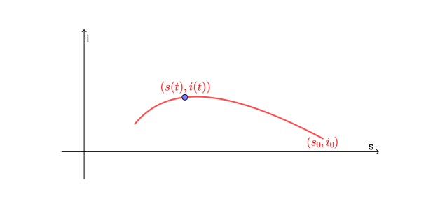
Figure 1: The epidemic trajectory

The following viability zones have been already defined in [4].

Definition 3.1

The set

$$\mathcal{B}:=\{(s_{0},i_{0})\in\mathbb{T}\ :\exists\,u\in U\mbox{ s.t.\ }i^{s_{0},i_{0},u}(t)\leq i_{M},\ \forall\,t\in I\}$$

is called feasible or viable set.

The set

$$\mathcal{A}:=\{(s_{0},i_{0})\in\mathbb{T}\ :i^{s_{0},i_{0},0}(t)\leq i_{M},\ \forall\,t\in I\}$$

is called no-effort or safe zone.

The viable set $\mathcal{B}$ is the maximal set of initial configurations on which at least one trajectory satisfies the constraint. When the epidemic initial state $(s_{0},i_{0})$ is inside $\mathcal{B}$, the epidemic is “under control”’. The safe zone $\mathcal{A}$ is the maximal set of initial configurations such that the associated uncontrolled trajectories satisfy the constraint. These sets play an important role in the synthesis of optimal control strategies.

The epidemic trajectories corresponding to constant controls are graphics $i=i(s)$ given by (2.6). Let us note that these functions are defined for every $s>0$, while the epidemic trajectory is only the part of the graph corresponding to $s\in(s_{\infty},s_{0}]$.

They are easy to study, and play a crucial role in the viability analysis. Given a prescribed (fixed) constant control $u$, and as $(s_{0},i_{0})$ varies, the family of graphs $\{s\mapsto i^{s_{0},i_{0},u}(s)\}_{(s_{0},i_{0})}$ satisfies the following properties (very easy to check).

1. Any graph of the family is strictly concave.

2. The graphs have all a unique maximum point in $\frac{\gamma}{\beta-u}$ (independent of $s_{0}$ and $i_{0}$).

3. Any graph goes from $(s_{0},i_{0})$ to $(s_{\infty},0)$ in infinite time (because $i$ is always strictly positive and $i_{\infty}=0$).

4. It is a laminar flow, that is, the graphs of the family are, two by two, disjoint or identically equal (recall that the control is constant and fixed). See the figure below for two laminar flows with different controls.

The figure shows some epidemic trajectories with constant controls. Of course only the arcs contained in the half plane of positive $i$ have physical meaning.

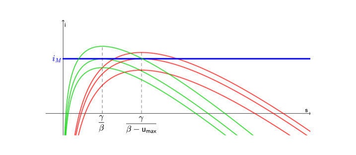
Figure 2: Epidemic trajectories with $u=0$ (in green) and $u=u_{\max}$ (in red)

The picture above suggests how to construct two relevant curves, $\Phi_{0}$ and $\Phi_{max}$, in black in the figure below.

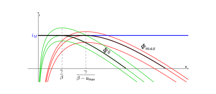
Figure 3: The curves $\Phi_{0}$ and $\Phi_{\max}$

They are obtained by glueing together the constant $i=i_{M}$ with the epidemic trajectories with $u=0$ and $u=u_{\max}$ and passing trough the maximum points

$$\big{(}\frac{\gamma}{\beta},i_{M}\big{)},\qquad\big{(}\frac{\gamma}{\beta-u_{\max}},i_{M}),$$

respectively, that is

$$\Phi_{0}(s) = \begin{cases}i_{M}&\mbox{if }0<s<\frac{\gamma}{\beta},\\ \frac{\gamma}{\beta}+i_{M}-s+\frac{\gamma}{\beta}\big{(}\log s-\log{\frac{\gamma}{\beta}}\big{)}&\mbox{if }s\geq\frac{\gamma}{\beta},\end{cases}$$

$$\Phi_{\max}(s) = \begin{cases}i_{M}&\mbox{if }0<s<\frac{\gamma}{\beta-u_{\max}},\\ \frac{\gamma}{\beta-u_{\max}}+i_{M}-s+\frac{\gamma}{\beta-u_{\max}}\big{(}\log s-\log{\frac{\gamma}{\beta-u_{\max}}}\big{)}&\mbox{if }s\geq\frac{\gamma}{\beta-u_{\max}}.\end{cases}$$

The region under the curve $\Phi_{max}$ is a viable set. Indeed, by choosing a point inside it and applying the maximum control $u=u_{\max}$ the corresponding trajectory stays always on, or strictly under, the curve $\Phi_{max}$ (due to the laminar flow property 4.; see the red curve under $\Phi_{\max}$ in Figure 3). If, instead, we start outside this region then the maximum control is not enough to take the epidemic curve under the level $i_{M}$ (always due to property 4.). To complete a formal proof of the claimed viability, it remains to prove that this last fact holds also for any other control (not only for $u=u_{\max}$). That is, the following characterization of the viable set holds.

Theorem 3.2

$\mathcal{B}=\{(s,i)\in\mathbb{T}\ :\ 0<i\leq\Phi_{\max}(s)\}.$

Proof. As we already remarked, the inclusion

$$\{(s,i)\in\mathbb{T}\ :\ 0<i\leq\Phi_{\max}(s)\}\subseteq\mathcal{B}$$

is trivially proven by choosing $u=u_{\max}$, and it remains only to prove the opposite inclusion.

Let us then consider $(s_{0},i_{0})\in\mathbb{T}$ and $u\in U$ be such such that $i^{s_{0},i_{0},u}\leq i_{M}$ for all $t\in I$. We have only to consider the case in which $s_{0}>\frac{\gamma}{\beta-u_{\max}}$ since, otherwise, $(s_{0},i_{0})\in\{(s,i)\in\mathbb{T}\ :\ 0<i\leq\Phi_{\max}(s)\}$ and the inclusion is proved. We aim to prove that $i_{0}\leq\Phi_{\max}(s_{0})$, that is

$$i_{0}\leq\frac{\gamma}{\beta-u_{\max}}+i_{M}-s_{0}+\frac{\gamma}{\beta-u_{\max}}\big{(}\log s_{0}-\log{\frac{\gamma}{\beta-u_{\max}}}\big{)}.$$ (3.1)

By Lemma 2.3, denoting by $i=i^{s_{0},i_{0},u}$ and $s=s^{s_{0},i_{0},u}$, we have

$$i_{0}=i(t)-s_{0}+s(t)-{\gamma}\int_{0}^{t}\frac{s^{\prime}(\tau)}{(\beta-u(\tau))s(\tau)}\,d\tau,\ \forall t\geq 0,$$

for every $t\geq 0$. Since $i\leq i_{M}$, by using $\frac{1}{\beta-u(\tau)}\leq\frac{1}{\beta-u_{\max}}$ and $\frac{s^{\prime}(\tau)}{s(\tau)}<0$ to estimate the integral, we get

$$i_{0}\leq i_{M}-s_{0}+s(t)-\frac{\gamma}{\beta-u_{\max}}\big{(}\log s(t)-\log s_{0}\big{)}.$$

which holds for every $t\geq 0$. Since, by point 3. of Proposition 2.4 and by continuity, we have that there exists $t_{\max}\geq 0$ such that $s(t_{\max})=\frac{\gamma}{\beta-u_{\max}}$, then the evaluation of the previuos inequality in $t=t_{\max}$ gives

$$i_{0}\leq i_{M}-s_{0}+\frac{\gamma}{\beta-u_{\max}}-\frac{\gamma}{\beta-u_{\max}}\big{(}\log\frac{\gamma}{\beta-u_{\max}}-\log s_{0}\big{)}$$

which is exactly (3.1). $\square$

Similarly, the region under the curve $\Phi_{0}$ is a safe zone. Indeed, by choosing a point inside it and applying the control $u=0$ the corresponding trajectory stays always on, or strictly under, the curve $\Phi_{0}$ (see the green curve under $\Phi_{0}$ in Figure 3). If, instead, we start outside this region then the control $u=0$ is not enough to take the epidemic curve under the level $i_{M}$, that is, the following characterization of the safe zone holds.

Theorem 3.3

$\mathcal{A}=\{(s,i)\in\mathbb{T}\ :\ 0<i\leq\Phi_{0}(s)\}.$

Remark 3.4

The previous theorems have been proven in [4, Theorem 2.3] by using viability tools. The proofs given here are elementary.

4 Greedy control strategy and examples

Starting from a point inside the viability set $\mathcal{B}$ and parametrizing by $s$ instead of $t$ (see Remark 2.8), the greedy control strategy consists in using for every $s$ the minimal control effort that takes the system inside the set $\mathcal{B}$; namely,

1. $u_{g}=0$ till the associated trajectory reaches a point on the curve $\Phi_{\max}$ and, afterwards, follow this curve till reaching herd immunity by using the following strategy

2. $u_{g}=u_{\max}$, as long as $s>\frac{\gamma}{\beta-u_{\max}}$,

3. $u_{g}=\beta-\frac{\gamma}{s}$, as long as $s\in(\frac{\gamma}{\beta},\frac{\gamma}{\beta-u_{\max}})$,

4. $u_{g}=0$, for every $s\geq\frac{\gamma}{\beta}$, that is, once that herd immunity has been reached.

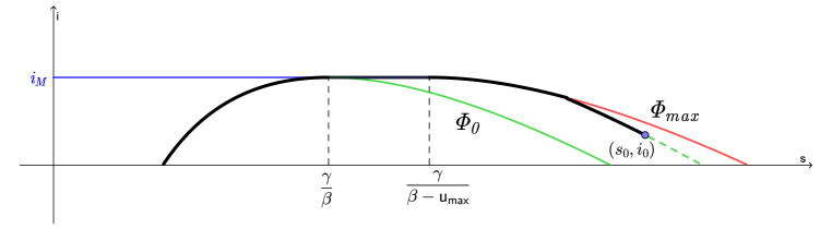
Figure 4: The greedy strategy (in black) starting from $(s_{0},i_{0})\in\mathcal{B}\setminus\mathcal{A}$

In particular, by applying the control 3. we have $i^{\prime}=0$ (by the second state equation), hence $i$ is taken at the level $i_{M}$ till to reach the herd immunity. Note that such control is admissible because it is an increasing function of $s$ on the interval $(\frac{\gamma}{\beta},\frac{\gamma}{\beta-u_{\max}})$ taking its minimum value $0$ in the left point $\frac{\gamma}{\beta}$ and maximum value $u_{\max}$ in the right point $\frac{\gamma}{\beta-u_{\max}}$.

A third important curve is the graph $\Psi_{0}$ displayed in Figure 5.

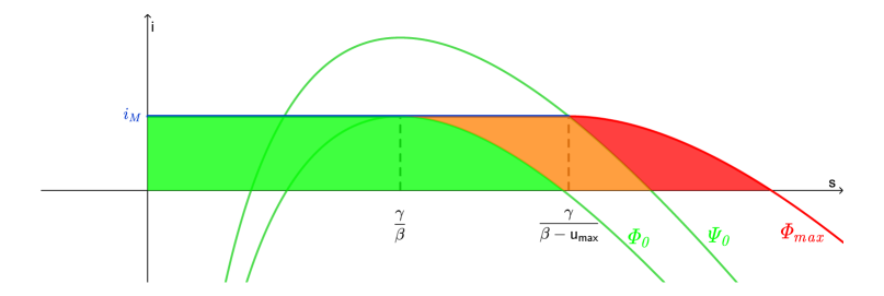
Figure 5: The curve $\Psi_{0}$

It is a curve travelled by control $u=0$ and passing trough the point $(\frac{\gamma}{\beta-u_{\max}},i_{M})$ and truncated at the level $i_{M}$, that is

$$\Psi_{0}(s)=\begin{cases}i_{M}&\mbox{if }0<s<\frac{\gamma}{{\beta-u_{\max}}},\\ \frac{\gamma}{\beta-u_{\max}}+i_{M}-s+\frac{\gamma}{\beta}\big{(}\log s-\log{\frac{\gamma}{\beta-u_{\max}}}\big{)}&\mbox{if }s\geq\frac{\gamma}{{\beta-u_{\max}}}.\end{cases}$$

It has the property that, starting from an initial point $(s_{0},i_{0})$ between $\Phi_{0}$ and $\Psi_{0}$ with control $u=0$, the level $i_{M}$ is reached without using the maximum control $u_{\max}$, that is, without imposing a lockdown. In the picture below, the safe zone $\mathcal{A}$ is coloured in green. The red zone corresponds to the points of $\mathcal{B}$ laying between the curves $\Psi_{0}$ and $\Phi_{\max}$ where a lockdown (i.e. $u=u_{\max}$) is needed.

Remark 4.1

The greedy strategy has been proved to be optimal (in [4, Theorem 5.6]) for the case of a cost functional depending only on the control (that is $\lambda_{2}=0$).

Remark 4.2

Along the greedy strategy, the herd immunity is always reached in finite time. This can be easily seen by observing that, starting from $(s_{0},i_{0})\in\mathcal{B}\setminus\mathcal{A}$, the curve $\Phi_{\max}$ is reached along a curve with control $u=0$ in finite time (indeed, the time to reach would be infinite only if the intersection point was $(s_{\infty}^{s_{0},i_{0},0},0)$, that is on the $s$ axis). Analogously, the time spent along the red part of the curve $\Phi_{\max}$ is finite or null. Finally, also the time eventually spent along the line $i=i_{M}$ can be computed (as well as in the other cases, by the way) by using the fact that, with the control given by 2. the first SIR equation becomes

$$\frac{ds}{dt}=-\gamma i_{M},$$

and, hence, the time spent along the line is, at most,

$$T_{\rm stab}=\int_{\frac{\gamma}{\beta-u_{\max}}}^{\frac{\gamma}{\beta}}\frac{dt}{ds}\,ds=-\int_{\frac{\gamma}{\beta-u_{\max}}}^{\frac{\gamma}{\beta}}\frac{1}{\gamma i_{M}}ds=\frac{u_{\max}}{\beta(\beta-u_{\max})i_{M}}.$$

The other times can be computed in an analogous way.

Example 4.3

To show examples we have to choose the epidemic parameters $\beta$, $\gamma$, $u_{\max}$, and the ICU threshold $i_{M}$. In this example we do it according to the available Covid-19 data in Italy at different times of the epidemic. In particular, we focus on the initial stage of March 2020 (mainly in Northern Italy) and on autumn 2021 when the government updated the control policies against the diffusion of the Delta variant.

According to [22] (see also [36]) which reports a range between $2.83$ and $3.10$, we take the basic reproduction number $R_{0}=3$. This value is a little bit more than the arithmetic average and takes into account the fact that the first part of the epidemic involved mainly the northern’s regions.

Moreover, by considering a time-to-recovery of 14 days ([6]), we get $\gamma=\frac{1}{14}\simeq 0.0714$ and hence $\beta=R_{0}\gamma\simeq 0.2142$.

About the numbers ICU places, $p_{\rm icu}$, an optimistic estimate is of $14$ over $100\,000$ inhabitants, which is, in fact, the Italian target after Decreto-Legge 19.05.2020 [17]. The reported critical cases in March 2020 was $c_{\rm icu}=4.5\%$ (see [27]). Hence, $i_{M}=\frac{p_{\rm icu}}{c_{\rm icu}}=0.0031$. The maximal control effort that we assume to be done is $u_{\max}=0.63\beta$, which corresponds to $63\%$ reduction of the transmission rate, according to the impact estimate of the lockdown on trasmissions given in [22].

The figure shows the viability zones for the previuos choice of the epidemic parameters (summarizing: $\gamma=0.0714$, $\beta=0.2142$, $i_{M}=0.0031$, $u_{\max}=0.135$) with an initial point $(s_{0},i_{0})=(0.94,0.001)$ that will be considered in the subsequent Example 10.2.

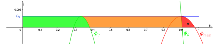
Figure 6: The viability zones at the initial stage of Covid-19 epidemic in Italy

In 2021 the Delta variant was more than two times transmissible than the ancestral Sars-CoV-2 virus (see for instance [31]). Accordingly, in this case, we choose $\beta=0.5$. With DL 23 Luglio 2021, n. 105, [18], the Italian government setted the alert level at 150 cases per $100\,000$ inhabitants. Since the time to recovery accredited by WHO was always (in mean) of $14$ days, we can estimate that the health system was considered able to support a number of infections $14$ times bigger, that is

$$i_{M}=14\frac{150}{100\,000}=0.021$$

possibly due also to the effect of the vaccinations that reduced the fraction of critical cases.

By updating data in this way (that is, by taking: $\gamma=0.0714$, $\beta=0.5$, $i_{M}=0.021$, $u_{\max}=0.315$), we obtain the following figure.

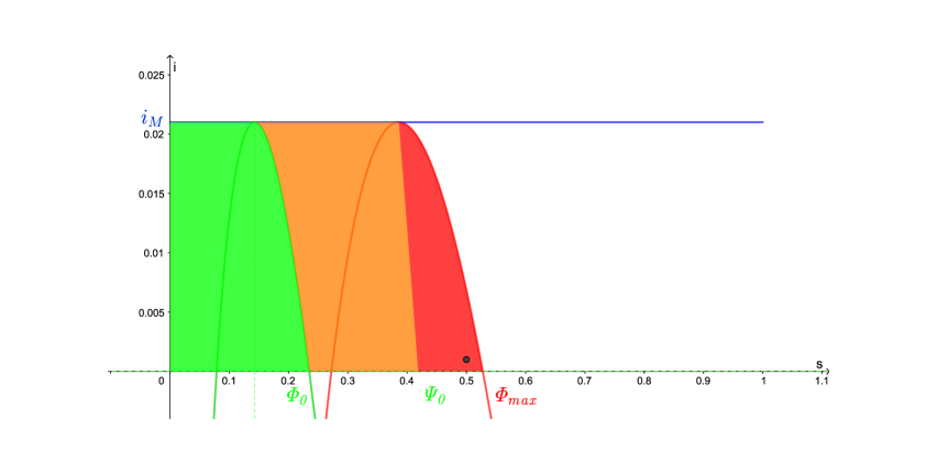
Figure 7: Viability zones for the Delta variant (autumn 2021) in Italy

The figure shows also the initial point $(s_{0},i_{0})=(0.5,0.001)$ that will be considered in the subsequent Example 10.3.

5 The optimal control problem for a general cost

The optimal control problem consists in minimizing a cost functional $J:U\times Y\to[0,\infty]$ of the form

$$J(u,s,i)=\int_{0}^{\infty}f_{0}(t,s,i,u)\,dt,$$ (5.1)

where $f_{0}$ is a given running cost such that the integral makes sense, over the set of state equations (1.1) with initial conditions $(s_{0},i_{0})$ in the viable set $\mathcal{B}$ and under the ICU constraint on the trajectories of (1.1)

$$i(t)\leq i_{M},\quad\forall t\in[0,+\infty).$$ (5.2)

An optimal solution to the control problem (5.1)-(5.2)-(1.1) is a vector function $(u,s,i)\in L^{\infty}(I;K)\times W^{1,\infty}(I;\mathbb{R}^{2})$ that minimizes the cost $J$ and satisfies the set of state equations and the upper bound on $i$. The function $u$ is an optimal control and $(s,i)$ an optimal state or trajectory. Accordingly, $U=L^{\infty}(I;K)$ is the space of controls and $Y=W^{1,\infty}(I;\mathbb{R}^{2})$ is the space of states.

The following semicontinuity and existence theorem for a very general cost functional holds.

Theorem 5.1

If $f_{0}:I\times\mathbb{R}^{2}\times\mathbb{R}\to[0,\infty)$ is a normal convex integrand, that is it is measurable with respect to the Lebesgue $\sigma$-algebra on $I$ and the Borel $\sigma$-algebra on $\mathbb{R}^{2}\times\mathbb{R}$ and there exists a subset $N\subset I$ of Lebesgue measure zero such that

1. $f_{0}(t,\cdot,\cdot,\cdot)$ is lower semicontinuous for every $t\in I\setminus N$,

2. $f_{0}(t,s,i,\cdot)$ is convex for every $t\in I\setminus N$ and $s,i\in\mathbb{R}$,

then

1. the cost functional $J$ defined by (5.1) is weakly* lower semicontinuous,

2. there exists an optimal solution $(u,s,i)$ to the control problem (5.1)-(1.1).

To prove the existence of an optimal solution we observe that it is equivalent to prove the existence of a minimizer of the functional

$$F(u,s,i):=J(u,s,i)+\chi_{\Lambda}(u,s,i)+\chi_{i\leq i_{M}}(i)$$ (5.3)

where $\Lambda$ is the set of admissible pairs, that is all state-control vectors $(u,s,i)$ that satisfy the initial value problem (1.1), while $\chi_{\Lambda}$ denotes the indicator function of $\Lambda$ that takes the value $0$ on $\Lambda$ and $+\infty$ otherwise; similarly, the function $\chi_{i\leq i_{M}}(i)$ is $0$ if $i(t)\leq i_{M}$ for every $t\in I$, and $+\infty$ otherwise.

Proof. By De Giorgi and Ioffe’s Theorem (see for instance [19, Theorem 7.5] or [13, Section 2.3]), for every $T\in(0,+\infty)$ the cost functional $J_{T}:L^{\infty}((0,T);K)\times W^{1,\infty}((0,T);\mathbb{R}^{2})\to[0,\infty]$ defined by

$$J_{T}(u,s,i)=\int_{0}^{T}f_{0}(t,s,i,u)\,dt$$

is weakly* lower semicontinuous. Then we obtain easily that also $J$ is lower semicontinuous. Indeed, given weakly* converging sequences $(s_{n},i_{n},u_{n})\stackrel{{\scriptstyle*}}{{\rightharpoonup}}(s,i,u)$, since the integrand is non-negative, we have

$$\int_{0}^{\infty}f_{0}(t,s,i,u)\,dt = \sup_{T>0}\int_{0}^{T}f_{0}(t,s,i,u)\,dt$$

$$\leq \sup_{T>0}\liminf_{n\to\infty}\int_{0}^{T}f_{0}(t,s_{n},i_{n},u_{n})\,dt$$

$$\leq \liminf_{n\to\infty}\int_{0}^{\infty}f_{0}(t,s_{n},i_{n},u_{n})\,dt.$$

This proves a. Let us now prove b. On the domain of $F$, that is the space $L^{\infty}(I;K)\times W^{1,\infty}(I;\mathbb{R}^{2})$, we consider the topology given by the product of the weak* topologies of the two spaces and aim to prove sequential lower semicontinuity and coercivity of the functional $F$ with respect to this topology. By the Direct Method of the Calculus of Variations (see, for instance, Buttazzo [13, Sec. 1.2]), these properties imply the existence of a solution to the minimum problem. They are direct consequences of the fact that the space of controls is weakly* compact, that the assumptions on $f_{0}$ imply that the cost functional $J$ is weakly* lower semicontinuous and the fact that the sets $\Lambda$ and $\{i\leq i_{M}\}$ are closed with respect to the weak* convergence. The claimed closedness of such sets follows by the application of Rellich compactness theorem, which ensures that weakly* converging sequences in $W^{1,\infty}(I)$ are, up to subsequences, uniformly converging on every bounded subset $J\subset I$ (see for instance [12, Theorem 8.8 and Remark 10]).

$\square$

Remark 5.2

The requirement on $f_{0}=f_{0}(t,s,i,u)$ to be a normal convex integrand is satisfied, in particular, if it is a piecewise continuous function of $t$, continuous in $(s,i)$ and convex in $u$.

6 The case of a linear cost

Problem 6.1

Given the initial data $(s_{0},i_{0})\in\mathcal{B}$ in the feasible region, minimize, over all admissible controls $u\in U$,

• the cost functional

  $$J^{\infty}(u,s,i)=\int_{0}^{\infty}\big{[}\lambda_{1}u(t)+\lambda_{2}i(t)\big{]}\,dt,$$ (6.1)

  with $\lambda_{2}\geq 0$, and $\lambda_{1}>0$,

• under the ICU constraint on the trajectory of (1.1)

  $$i(t)\leq i_{M},\quad\forall t\in[0,+\infty).$$ (6.2)

In the sequel, we refer to this formulation as problem $\mathcal{P}^{\infty}_{{\lambda_{1}},{\lambda_{2}}}$.

Remark 6.1

Non-emptiness of the set of viable controls with a corresponding finite cost is guaranteed by using, for example, the greedy strategy, $u_{g}$, described in Section 4 till the herd immunity is reached, and $u_{g}=0$ afterwards. Indeed, as observed in Remark 4.2, with this strategy the herd immunity is reached in finite time. Hence, there exists $t_{I}\geq 0$ such that $s(t_{I})\leq\frac{\gamma}{\beta}$ and $u_{g}=0$ in $(t_{I},+\infty)$. Moreover, since $s$ is strictly decreasing, there exists $\varepsilon>0$ and $t_{\varepsilon}\geq t_{I}$ such that $s(t)\leq\frac{\gamma}{\beta}-\varepsilon$ for every $t\in(t_{\varepsilon},+\infty)$ and hence

$$\beta s(t)-\gamma\leq-\varepsilon\beta.$$

Thus, for every $t\in(t_{\varepsilon},+\infty)$, we have

$$i(t)=i_{\varepsilon}{\mathop{\rm e}\nolimits}^{\int_{t_{\varepsilon}}^{t}[\beta s(\tau)-\gamma]\,d\tau}\leq i_{I}{\mathop{\rm e}\nolimits}^{-\varepsilon\beta(t-t_{\varepsilon})}.$$

Then we have

$$\int_{t_{\varepsilon}}^{\infty}i(t)\,dt<+\infty,$$

and this implies

$$J^{\infty}(u,s,i)=\int_{0}^{\infty}\big{[}\lambda_{1}u(t)+\lambda_{2}i(t)\big{]}\,dt=\int_{0}^{t_{\varepsilon}}\big{[}\lambda_{1}u(t)+\lambda_{2}i(t)\big{]}\,dt+\lambda_{2}\int_{t_{\varepsilon}}^{\infty}i(t)\,dt<+\infty.$$

Proposition 6.2

For every $\left(s_{0},i_{0}\right)\in\mathcal{B}$ with $i_{0}>0$ the problem $\mathcal{P}_{{\lambda_{1}},{\lambda_{2}}}^{\infty}$ has an optimal solution with a finite cost.

Proof. Follows by Theorem 5.1, by taking into account that Remark 6.1 ensures that there exists at least an admissible pair $(u,s,i)$ with a finite cost. $\square$

Very important for our analysis is that, with an infinite time horizon, to reach herd immunity in finite time is a necessary condition for optimality. Indeed, the following consequence of Theorem 2.6 holds true.

Corollary 6.3

If $u$ is an optimal control for problem $\mathcal{P}_{{\lambda_{1}},{\lambda_{2}}}^{\infty}$, then $s^{u}_{\infty}<\frac{\gamma}{\beta}$.

Proof. By Theorem 2.6, it is enough to observe that $u\in L^{1}(I)$. In fact, this is a consequence of the fact that optimal controls have a finite cost (see Proposition 6.2), and of the inequality

$$\int_{0}^{\infty}u\,dt\leq\frac{1}{\lambda_{1}}J^{\infty}(u,s,i)<\infty.$$

$\square$

7 Reduction to finite horizon problems

Besides the elements already discussed in the previous section (Corollary 6.3), other optimality conditions can be stated by using Pontryagin’s theorem on finite horizon problems suitably related to the (infinite horizon) original problem.

Problem 7.1

Let $T>0$. Given the initial data $(s_{0},i_{0})\in\mathcal{B}$ in the feasible region, minimize, over all admissible controls $u\in{L}^{\infty}\big{(}(0,T);[0,u_{\max}]\big{)}$,

• the cost functional

  $$J^{T}(u,s,i)=\int_{0}^{T}\big{[}\lambda_{2}i(t)+\lambda_{1}u(t)\big{]}\,dt,$$ (7.1)

  with $\lambda_{2}\geq 0$ and $\lambda_{1}>0$,

• under the ICU constraint on the trajectory of (1.1)

  $$i(t)\leq i_{M}\quad\forall t\in[0,T].$$ (7.2)

In the sequel, we refer to this formulation as problem $\mathcal{P}^{T}_{{\lambda_{1}},{\lambda_{2}}}$.

Let us remark that when $T=\infty$ we obtain the infinite horizon problem $\mathcal{P}^{\infty}_{{\lambda_{1}},{\lambda_{2}}}$ already introduced as Problem 6.1.

Assume $u\in U$ to be an optimal control for problem $\mathcal{P}^{\infty}_{{\lambda_{1}},{\lambda_{2}}}$. By Corollary 6.3, we have $s_{\infty}^{u}<\frac{\gamma}{\beta}$, hence the time $T^{u}_{\frac{\gamma}{\beta}}$, to reach the herd immunity level $s^{u}=\frac{\gamma}{\beta}$ with the control $u$, turns out to be finite. If $\lambda_{2}=0$, after time $T^{u}_{\frac{\gamma}{\beta}}$ the optimal control is identically $0$, because $i$ is decreasing and the ICU constraint is trivially satisfied, and any other choice of $u$ would lead to a bigger cost. This allows to use the finite horizon problem on $[0,T]$ to state other necessary (Pontryagin) optimality conditions in the case $\lambda_{2}=0$. Unfortunately, the same argument cannot be used if $\lambda_{2}>0$. Nevertheless, it will be shown that a reduction to finite horizon problems can be obtained by a $\Gamma$-convergence argument, covering also the case $\lambda_{2}>0$.

7.1 The case of a cost depending only on the control ($\lambda_{2}=0$)

In the case $\lambda_{2}=0$ the following reduction theorem holds.

Theorem 7.1 (Reduction to a finite horizon, case $\boldsymbol{\lambda_{2}=0}$)

Let $u\in U$ be an optimal control for problem $\mathcal{P}^{\infty}_{{\lambda_{1}},{\lambda_{2}}}$. If $\lambda_{2}=0$ then, for every $T>T^{u}_{\frac{\gamma}{\beta}}$, the restriction $u_{|}:=u_{|[0,T]}$ is an optimal control for the finite horizon problem $\mathcal{P}^{T}_{{\lambda_{1}},{\lambda_{2}}}$ with target objective $s(T)<\frac{\gamma}{\beta}$.

Proof. By contradiction, assume that $u_{|}$ is not optimal. Then there exists ${\bar{u}}\in L^{\infty}((0,T);[0,u_{\max}])$ with $s^{\bar{u}}(T)<\frac{\gamma}{\beta}$ and such that

$$J^{T}({\bar{u}},s^{\bar{u}},i^{\bar{u}})<J^{T}(u_{|},s^{u_{|}},i^{u_{|}}).$$

Denoting by ${\bar{u}}_{0}$ the extension of ${\bar{u}}$ to the interval $(0,+\infty)$ by setting it to zero after $T$, using the local property of the systems of differential equations, we would have $i^{\bar{u}}=i^{{\bar{u}}_{0}}_{|[0,T]}$, and $s^{\bar{u}}=s^{{\bar{u}}_{0}}_{|[0,T]}$. Then, in particular, $s^{{\bar{u}}_{0}}(T)=s^{\bar{u}}(T)<\frac{\gamma}{\beta}$. This implies

$$J^{\infty}({\bar{u}}_{0},s^{{\bar{u}}_{0}},i^{{\bar{u}}_{0}})=\int_{0}^{T}\lambda_{1}{\bar{u}}\,dt=J^{T}({\bar{u}},s^{\bar{u}},i^{\bar{u}})<J^{T}(u_{|},s^{u_{|}},i^{u_{|}})\leq J^{\infty}(u,s^{u},i^{u}),$$

which contradicts the optimality of $u$. $\square$

Since, by Corollary 6.3, $T^{u}_{\frac{\gamma}{\beta}}$ is finite, then the infinite horizon optimal control problem is brought back to a finite horizon OCP with a target objective. The latter has been studied in [4, 3] and the structure of the (unique) optimal control has been characterized. According to Theorem 5.6 of [4], the greedy strategy is optimal also in the case of an infinite horizon (and without any target objective). This explains also what has been observed by Molina & Rapaport, in the introduction to [34], when they compare their result with those obtained in [4].

7.2 The general case

When the cost depends also from $i$, which, differently from the control, vanishes only as $t\to\infty$, the argument used before does not work. Nevertheless, in this section we show that (even when $\lambda_{2}>0$) a reduction to finite horizon problems can be obtained by a $\Gamma$-convergence argument. $\Gamma$-convergence is a general notion of variational convergence introduced in 1976 by De Giorgi and Franzoni [15, 16]; we refer the unaccustomed reader also to the books of Dal Maso [14] and Braides [11] for general properties and selected applications. To shorten notation, throughout this section all problems refer to the same fixed intial data $(s_{0},i_{0})$ in the viable set ${\mathcal{B}}$.

Theorem 7.2

For every increasing sequence of positive numbers $T_{n}\to\infty$, the sequence of problems $\mathcal{P}^{T_{n}}_{{\lambda_{1}},{\lambda_{2}}}$ $\Gamma$-converges to the limit problem $\mathcal{P}^{\infty}_{{\lambda_{1}},{\lambda_{2}}}$ in the following sense:

1. (liminf inequality) for every sequence $u_{n}\in U$ with $i^{u_{n}}\leq i_{M}$, $u_{n}=0$ on $(T_{n},+\infty)$, and $u_{n}\stackrel{{\scriptstyle*}}{{\rightharpoonup}}u$ in $L^{\infty}(I)$ we have $i^{u}\leq i_{M}$ and

   $$\liminf_{n\to\infty}J^{T_{n}}(u_{n},s^{u_{n}},i^{u_{n}})\geq J^{\infty}(u,s^{u},i^{u});$$

2. (recovery sequence) for every $u\in U$ with $J^{\infty}(u,s^{u},i^{u})<\infty$ with $i^{u}\leq i_{M}$, there exists $u_{n}\in U$ with $i^{u_{n}}\leq i_{M}$, $u_{n}=0$ on $(T_{n},+\infty)$, and $u_{n}\stackrel{{\scriptstyle*}}{{\rightharpoonup}}u$ in $L^{\infty}(I)$ such that

   $$\lim_{n\to\infty}J^{T_{n}}(u_{n},s^{u_{n}},i^{u_{n}})=J^{\infty}(u,s^{u},i^{u}).$$

Remark 7.3

1. The statement of Theorem 7.2 can also be written in terms of usual $\Gamma$-convergence as $T\to\infty$ with respect to the weak* convergence on the space $L^{\infty}(I;[0,u_{\max}])\times W^{1,\infty}(I;\mathbb{R}^{2})$ of the family of functionals

   $$F^{T}(u,s,i):=J^{T}(u,s,i)+\chi_{\Lambda}(u,s,i)+\chi_{i\leq i_{M}}(i)+\chi_{u=0\mbox{ in }(T,+\infty)}(u)$$

   to the $\Gamma$-limit functional

   $$F^{\infty}(u,s,i):=J^{\infty}(u,s,i)+\chi_{\Lambda}(u,s,i)+\chi_{i\leq i_{M}}(i).$$

2. The condition $u_{n}=0$ in $(T_{n},+\infty)$ does not affect the problem $\mathcal{P}^{T_{n}}_{{\lambda_{1}},{\lambda_{2}}}$; indeed, after $T_{n}$ the control can be set at any desired value without changing the value of the optimal control problem on the finite horizon $[0,T_{n}]$.

Lemma 7.4

If $u_{n}\stackrel{{\scriptstyle*}}{{\rightharpoonup}}u$ in $L^{\infty}(I;[0,u_{\max}])$, then $s^{u_{n}}\to s^{u}$ and $i^{u_{n}}\to i^{u}$ uniformly on every bounded subinterval $J\subset I$.

Proof. Since $u_{n}$, $s^{u_{n}}$ and $i^{u_{n}}$ are uniformly bounded, the derivatives of $s^{u_{n}}$ and $i^{u_{n}}$ are uniformly bounded as well. Hence, $\|s^{u_{n}}\|_{1,\infty}$ and $\|i^{u_{n}}\|_{1,\infty}$ are bounded. Then the sequence $(s^{u_{n}},i^{u_{n}})$ is contained in a ball $B$ of the space $W^{1,\infty}(I;\mathbb{R}^{2})$ on which (by the separability of $L^{1}$) the weak* topology is metrizable. Since bounded sets are weakly* relatively compact, then any subsequence of $(s^{u_{n}},i^{u_{n}})$ admits a weakly* converging subsequence. The application of Rellich compactness theorem ensures that weakly* converging sequences in $W^{1,\infty}(I;\mathbb{R}^{2})$ are, up to subsequences, uniformly converging on every bounded subset $J\subset I$ (see for instance [12, Theorem 8.8 and Remark 10]). We are then allowed to pass to the limit in the state equations and, using the uniqueness of the solution, we get that these subsequence converges to $(s^{u},i^{u})$. Since the limit is always the same and we are inside a metrizable set, then we can conclude that the whole sequence converges to these limit. Hence, $(s^{u_{n}},i^{u_{n}})\stackrel{{\scriptstyle*}}{{\rightharpoonup}}(s^{u},i^{u})$ in $W^{1,\infty}(I;\mathbb{R}^{2})$. The claimed uniform convergence on bounded subintervals comes again form the application of Rellich’s theorem. $\square$

Proof. (of Theorem 7.2). 1. By the previous lemma, the convergence assumption $u_{n}\stackrel{{\scriptstyle*}}{{\rightharpoonup}}u$ in $L^{\infty}(I;[0,u_{\max}])$ implies that $i^{u_{n}}$ converges to $i^{u}$ uniformly on the bounded subintervals of $I$, and this implies $i^{u}\leq i_{M}$. Let us now remark that

$$\liminf_{n\to\infty}\int_{0}^{T_{n}}i^{u_{n}}=\liminf_{n\to\infty}\int_{0}^{\infty}i^{u_{n}}1_{[0,T_{n}]}\,dt\geq\int_{0}^{\infty}i^{u}\,dt$$

simply by using the fact that the sequence $i^{u_{n}}1_{[0,T_{n}]}$ pointwisely converges to $i^{u}$ on $(0,+\infty)$ and Fatou’s lemma (see, for instance, [35, Theorem 11.31]).

By using the fact that $u_{n}=0$ on $(T_{n},+\infty)$, the semicontinuity part a.  of Theorem 5.1 applied to the function $f_{0}(t,u,s,i)=u$, and the last inequality, we get

$$\begin{split}\liminf_{n\to\infty}J^{T_{n}}(u_{n},s^{u_{n}},i^{u_{n}})=&\liminf_{n\to\infty}\int_{0}^{T_{n}}\lambda_{1}u_{n}+\lambda_{2}i^{u_{n}}\,dt\\ =&\lambda_{1}\liminf_{n\to\infty}\int_{0}^{\infty}u_{n}\,dt+\lambda_{2}\liminf_{n\to\infty}\int_{0}^{T_{n}}i^{u_{n}}\,dt\\ \geq&\int_{0}^{\infty}\lambda_{1}u+\lambda_{2}i^{u}\,dt=J^{\infty}(u,s^{u},i^{u}).\end{split}$$ (7.3)

2. It remains to prove the existence of a recovery sequence. It can be constructed as follows. Since $J^{\infty}(u,s^{u},i^{u})<\infty$, the control $u$ belongs to $L^{1}(I)$ and, hence, $s_{\infty}^{u}<\frac{\gamma}{\beta}$, by Proposition 2.6.

Let us define

$$u_{n}(t)=\begin{cases}u(t)&\mbox{ if }t\in(0,T_{n}),\\ 0&\mbox{ if }t\in(T_{n},+\infty).\end{cases}$$

Since $T_{n}\to\infty$, for every $n$ large enough we have $s^{u_{n}}(T_{n})=s^{u}(T_{n})<\frac{\gamma}{\beta}$. This implies that $i^{u_{n}}\leq i_{M}$. Indeed, before time $T_{n}$, we have $i^{u_{n}}=i^{u}\leq i_{M}$, while for every time after the function $i^{u_{n}}(\cdot)$ is decreasing.

Moreover, $u_{n}\stackrel{{\scriptstyle*}}{{\rightharpoonup}}u$ in $L^{\infty}(I)$ (by Lebesgue’s theorem). Finally, by monotone convergence we have

$$\lim_{n\to\infty}J^{T_{n}}(u_{n},s^{u_{n}},i^{u_{n}}) = \lim_{n\to\infty}\int_{0}^{T_{n}}\lambda_{2}i^{u_{n}}+\lambda_{1}u_{n}\,dt$$ (7.4)

$$= \int_{0}^{\infty}\lambda_{2}i^{u}+\lambda_{1}u\,dt=J^{\infty}(u,s^{u},i^{u})$$ (7.5)

and the theorem is completely proved. $\square$

The next theorem is a consequence of the variational property of $\Gamma$-convergence.

Theorem 7.5

Let $u_{T}$ be an optimal control for $\mathcal{P}^{T}_{{\lambda_{1}},{\lambda_{2}}}$ with $T<\infty$, extended by $0$ in $(T,+\infty)$. Then

1. there exists an increasing sequence $T_{n}\to\infty$ and $u\in U$ such that $u_{T_{n}}\stackrel{{\scriptstyle*}}{{\rightharpoonup}}u$;

2. if $(T_{n})$ is sequence of positive numbers such that $T_{n}\to\infty$ and $u_{T_{n}}\stackrel{{\scriptstyle*}}{{\rightharpoonup}}u$, then $u$ is an optimal control for problem $\mathcal{P}^{\infty}_{{\lambda_{1}},{\lambda_{2}}}$.

Proof. The first part of the statement immediately follows by the fact that $(u_{T})$ is an equi-bounded family in $L^{\infty}(I)$ and the existence of a weak* converging sequence follows by Alaoglu’s theorem.

About assertion 2., by using Theorem 2.1, it is easily seen that the optimal pair $(u_{T_{n}},s^{u_{T_{n}}},i^{u_{T_{n}}})$ weakly* converges in $U\times Y$ to $(u,s^{u},i^{u})$, and the claim follows by the variational property of $\Gamma$-convergence (see, for instance, [14, Corollary 7.17]). $\square$

Remark 7.6

The $\Gamma$-convergence Theorem 7.2 and its consequence Theorem 7.5 allow us to deal with finite horizon problems. Indeed, suppose that $u_{n}$ is an optimal control for problem $\mathcal{P}^{T_{n}}_{{\lambda_{1}},{\lambda_{2}}}$ (which exists), extended by $0$ on $[T_{n},+\infty)$. Since $U$ is weakly* compact, then, up to a subsequence, $u_{n}\stackrel{{\scriptstyle*}}{{\rightharpoonup}}u$ and $u$ is optimal for $\mathcal{P}^{\infty}_{{\lambda_{1}},{\lambda_{2}}}$.

Since $u$ is optimal, then $s^{u}_{\infty}<\frac{\gamma}{\beta}$ (see Corollary 6.3) and, therefore, there exists $\varepsilon>0$ and $T_{\varepsilon}\in[0,+\infty)$ such that $s^{u}(t)<\frac{\gamma}{\beta}-\varepsilon$ for every $t>T_{\varepsilon}$.

On the other hand, by Lemma 7.4, $u_{n}\stackrel{{\scriptstyle*}}{{\rightharpoonup}}u$ implies $s^{u_{n}}(T_{\varepsilon})\to s^{u}(T_{\varepsilon})$. Hence, there exists $n_{\varepsilon}\in\mathbb{N}$ such that $s^{u_{n}}(t)<\frac{\gamma}{\beta}$ for every $t>T_{\varepsilon}$ and $n>n_{\varepsilon}$. Since $T_{n}\to\infty$, then, possibly increasing $n_{\varepsilon}$, we have $T_{n}>T_{\varepsilon}$ for every $n>n_{\varepsilon}$. Hence $s^{u_{n}}(T_{n})<\frac{\gamma}{\beta}$ for every $n>n_{\varepsilon}$.

We are, essentially, saying that for any $T$ large enough, the optimal control $u_{T}$ of $\mathcal{P}^{T}_{{\lambda_{1}},{\lambda_{2}}}$ satisfies the final condition $s^{u_{T}}(T)<\frac{\gamma}{\beta}$. We are, then, led to characterize the optimal controls for such $T$ large enough being allowed, in doing it, to use the final condition $s(T)<\frac{\gamma}{\beta}$ as a necessary condition (not as an assumption). As already explained in the introduction, this necessary optimality condition has a very important simplifying consequence in the application of Pontryagin’s principle, because it implies normality (this will become clear in the proof of Theorem 9.1 and 9.7).

8 The finite horizon problem: optimality conditions

8.1 Pontryagin approach. General considerations

To write necessary conditions of optimality let us introduce the adjoint variables $p_{0}\geq 0$, $p_{s},p_{i}\in\mathbb{R}$, and the pre-Hamiltonian

$$H(t,u,s,i,p_{0},p_{s},p_{i})=p_{0}f_{0}(s,i,u)+p_{s}f_{s}+p_{i}f_{i},$$

where $f_{0}(s,i,u)=\lambda_{2}i+\lambda_{1}u$ is the running cost function and $f_{s}=-s(\beta-u)i$, $f_{i}=s(\beta-u)i-\gamma i$ are the dynamics of the state equations. After some manipulations, the pre-Hamiltonian turns out to be

$$H(t,u,s,i,p_{0},p_{s},p_{i})=p_{0}(\lambda_{2}i+\lambda_{1}u)+\eta s(\beta-u)i-\gamma p_{i}i,$$

where

$$\eta:=p_{i}-p_{s}.$$

In the sequel we use a constrained version of Pontryagin’s theorem developed in [10, 9]. In particular, we refer to [9] for the definition of the space of functions with bounded variation $BV([0,T])$ which is given by extending functions in a constant way on an open interval containing $[0,T]$. We adopt here also the notation used in [10, 9] of denoting the distributional derivative of a $BV$ function $f$ (which is a measure) by $df$, instead than $f^{\prime}$ that we reserve to measures which are absolutely continuous with respect to Lebesgue as, for instance, in the state equations.

8.2 Optimality conditions for problem ${\mathcal{P}}^{T}_{\lambda_{1},\lambda_{2}}$ with $T<\infty$

By Pontryagin’s theorem, given an optimal solution $(s,i,b)$, there exist a constant $p_{0}\in\{0,1\}$, adjoint state real functions $p_{s},\,p_{i}\in BV([0,T])$, a multiplier for the state constraint $\mu\in BV([0,T])$ with a nondecreasing representative (hence with measure distributional derivative $d\mu\geq 0$) such that $\mu(T^{+})=0$ (recall that the functions are extended outside $[0,T]$), that satisfy the following properties.

• The non-degeneration property

  $$p_{0}+d\mu([0,T])>0.$$ (8.1)

• The complementarity condition

  $$\int_{[0,{T}]}\big{(}i(t)-i_{M})\ d\mu(t)=0.$$ (8.2)

• The conjugate equations with transversality conditions

  $$\begin{cases}dp_{s}=-\eta(\beta-u)i,\\ dp_{i}=-\big{(}p_{0}\lambda_{2}+\eta(\beta-u)s-\gamma p_{i}\big{)}-d\mu,\\ p_{s}(T)=0,\ p_{i}(T^{+})=0,\end{cases}$$

  which hold as equalities between measures on $[0,T]$. We observe that the boundary condition for the costate $p_{i}$ is given on the right limit in $T$, since $p_{i}$ could be discontinuous in $T$ if the measure $d\mu$ charges this point. On the contrary, $p_{s}$ is continuous in $[0,T]$ since the derivative is absolutely continuous with respect to the Lebesgue measure.

• The minimality property

  $$H\big{(}t,u(t),s(t),i(t),p_{0},p_{s}(t),p_{i}(t)\big{)}=\inf_{u\in[0,u_{\max}]}\!H\big{(}t,u,s(t),i(t),p_{0},p_{s}(t),p_{i}(t)\big{)},$$

  for almost every $t\in[0,T]$.

• The conservation property

  $$H\big{(}t,u(t),s(t),i(t),p_{0},p_{s}(t),p_{i}(t)\big{)}=k,$$

  with $k$ constant, for a.e.  $t\in[0,T]$ (see [8, Lemma 7.7]).

8.3 Remarks and consequences

Throughout all this section we assume that $(s=s^{s_{0},i_{0},u},i=i^{s_{0},i_{0},u},u)$ be a solution of the control Problem 7.1 with initial data $(s_{0},i_{0})\in\mathcal{B}$ and write consequences of Pontryagin’s necessary conditions. Here we assume, moreover, that $s(T)<\frac{\gamma}{\beta}$; for our problem, this is not a restriction as observed in Remark 7.6.

We have the following consequences.

• By (P3) and the definition of $\eta$ the jump condition $[\eta(t)]=[p_{i}(t)]=-[\mu(t)]\leq 0$ holds for every $t\in[0,T]$ (where the jump of a BV function $f$ in a point $t$ is defined by $[f(t)]:=\displaystyle\lim_{s\to t^{+}}f(s)-\displaystyle\lim_{s\to t^{-}}f(s)=df(\{t\})$ and the inequality follows by the fact that $\mu$ is non-decreasing).

• By the conservation of the Hamiltonian

  $$p_{0}\big{(}\lambda_{2}i(t)+\lambda_{1}u(t)\big{)}+\eta(t)\big{(}\beta-u(t)\big{)}s(t)i(t)-\gamma p_{i}(t)i(t)=k,\mbox{ for a.e.\ }t\in[0,T].$$ (8.3)

• (P3) implies that

  $$d\eta=dp_{i}-dp_{s}=\eta(\beta-u)(i-s)-p_{0}\lambda_{2}+\gamma p_{i}-d\mu,$$ (8.4)

  or, owing to (8.3),

  $$d\eta=\eta(\beta-u)i+\frac{p_{0}\lambda_{1}u-k}{i}-d\mu.$$ (8.5)

• Since $s(T)<\frac{\gamma}{\beta}$ and $s$ is continuous, we have that $s<\frac{\gamma}{\beta}$ in an interval $(t_{I},T]$ with $t_{I}<T$. This implies that $i^{\prime}=\big{(}s(\beta-u)-\gamma\big{)}i<-\frac{\gamma}{\beta}ui\leq 0$, hence $i$ is decreasing and therefore $i<i_{M}$ in $(t_{I},T]$. Then, by complementarity, we have $d\mu((t_{I},T])=0$ which implies that $p_{i}$, and thus $\eta$ and $\psi$, are continuous in $(t_{I},T]$. This implies $p_{i}(T)=0$ and $\eta(T)=0$.

Since the cost is linear in the control $u$, the minimum value of the Hamiltonian on $K=[0,u_{\max}]$ is achieved when $u\in\{0,u_{\max}\}$. Hence, setting the switching function

$$\psi:=\eta si,$$

the optimal control has to satisfy

$$b(t)=\begin{cases}0,&\textnormal{ if }\psi(t)<p_{0}\lambda_{1},\\[0.0pt] u_{\max},&\textnormal{ if }\psi(t)>p_{0}\lambda_{1},\end{cases}$$ (8.6)

for almost every $t\in[0,T]$, where $\psi$ denotes any pointwise representative of the switching function. By $(C_{4})$, we note that $\psi(T)=0$.

The criterium (8.6) allows to compute the value of $k$ in (8.3).

Proposition 8.1

In (C2) we have $k=p_{0}\lambda_{2}i(T)$.

Proof. By having (C4) in mind, let us distinguish two cases.

1. If $p_{0}=1$ then $\psi(T)=0<p_{0}\lambda_{1}$ and, by continuity, we have $\psi(t)<p_{0}\lambda_{1}$ and hence $u(t)=0$ a.e. in a left neighborhood of $T$ which we still call $(t_{I},T]$; (8.3) implies

   $$k=p_{0}\lambda_{2}i(t)+\eta(t)\beta s(t)i(t)-\gamma p_{i}(t)i(t)\ \mbox{a.e.\ }t\in(t_{I},T],$$

   and, by taking the limit as $t\rightarrow T-$, and invoking (C4), we obtain

   $$k=p_{0}\lambda_{2}i(T).$$

2. If $p_{0}=0$ then (8.3) implies

   $$k=\eta(t)\big{(}\beta-u(t)\big{)}s(t)i(t)-\gamma p_{i}(t)i(t)\ \mbox{a.e.\ }t\in(t_{I},T].$$ (8.7)

   By taking a sequence $t_{n}\to T$ on which the equality (8.7) holds and passing to the limit as $n\to\infty$ then we get $k=0$, which proves the proposition also in this case.

$\square$

Proposition 8.2

$\eta(t)\geq 0$ for almost every $t\in[0,T]$.

Proof. Let us recall that, by (C4), $\eta$ is continuous in a left neighborhood of $T$ and $\eta(T)=0$.

We note that, since $\mu$ is nondecreasing, $d\mu\geq 0$ and, therefore, (8.5) implies

$$d\eta\leq\eta(\beta-u)i+\frac{p_{0}\lambda_{1}u-k}{i}.$$ (8.8)

Without loss of generality, we assume $\eta$, and thus $\psi$, to be right-continuous. Moreover $\eta$, and thus $\psi$, cannot have increasing jumps (by $(C1)$).

Arguing by contradiction, let us assume that there exists $t\in(0,t_{0})$ such that $\eta(t)=\eta(t^{+})<0$. Since the switching function $\psi=\eta si$ has the same sign as $\eta$, and since $p_{0}\geq 0$, we have $\psi(t^{+})<p_{0}\lambda_{1}$. On the other hand, since $\psi$ is right-continuous, one is able to find some $\varepsilon>0$ such that $\psi<p_{0}\lambda_{1}$, and hence $u=0$, a.e.  in $J:=(t,t+\varepsilon)$. Owing to (8.8) with $u=0$, in $J$ we have

$$d\eta\leq\eta\beta i-\frac{k}{i}.$$

Since $k\geq 0$ (see Proposition 8.1) , we have that

$$d\eta\leq\eta\beta i$$

and $\eta\beta i<0$ in $J$, and therefore $\eta$ is negative and strictly decreasing in $J$.

As we shall see, this implies that $\eta<0$, and strictly decreasing, in $(t,T)$, which implies $\eta(T)<0$, thus contradicting the fact that $\eta(T)=0$.

To prove the claim that $\eta<0$ in $(t,T)$, let us set

$$t_{1}:=\sup\{s\in(t,T]\ :\ \eta(s)<0\}.$$

(recall that $\eta$ is assumed to be right-continuous). Assume, again by contradiction, that $t_{1}<T$. Since $\eta\in BV$, then there exists the left limit $\eta(t_{1}^{-})\leq 0$. Since $\eta$ has no positive jumps in $[0,T]$, it follows that $\eta(t_{1}^{+})\leq 0$. On the other hand, $\eta(t_{1}^{+})<0$ would contradict the definition of $t_{1}$. It follows that $\eta(t_{1})=0$. Nevertheless, in the interval $(t,t_{1})$ we have that $\eta<0$, hence $\psi<0$. Then, in $(t,T)$ we have that $\psi<p_{0}\lambda_{1}$, hence $u=0$ a.e., hence $d\eta\leq\eta(\beta-u)i<0$, hence $\eta$ is decreasing, which contradicts $\eta(t_{1})=0$. Our assumption on $t_{1}$ is wrong such that $t_{1}=T$ and $\eta<0$ in $(t,T)$. As we have already indicated, this contradicts $\eta(T)=0$ and, hence, our Proposition follows. $\square$

Corollary 8.3

1. $\psi$ is non-negative almost everywhere in $(0,T)$;

2. $p_{s}$ is continuous, non-increasing and non-negative in $[0,T]$.

Proof. It is a straightforward consequence of the non-negativity of $\eta$, of the definition of $\psi$, of the first adjoint equation and the final condition $p_{s}(T)=0$. $\square$

Using (8.4), one easily proves the following result.

Proposition 8.4

The distributional derivative of $\psi$ is the measure given by

$$d\psi=si(\gamma p_{s}-p_{0}\lambda_{2})-si\,d\mu.$$

The next theorem provides a characterization of singular arcs, whenever they occur.

Theorem 8.5

Let $(t_{1},t_{2})\subset\left[0,T\right]$ be an interval in which $\psi=p_{0}\lambda_{1}$. Then the following hold true

1. if $p_{0}=1$, then $\gamma p_{s}(t)-\lambda_{2}>0$ and $i(t)=i_{M}$, for every $t\in(t_{1},t_{2})$;

2. if $p_{0}=0$, then $\eta=p_{i}=p_{s}=0,$ in $(t_{1},T]$ and $d\mu([0,t_{1}])>0$.

Proof. Let us consider the case when $p_{0}=1$ and prove the first assertion. First of all, since $\psi=\eta si=p_{0}\lambda_{1}>0$, then we have $\eta>0$ in $(t_{1},t_{2})$. Since $\psi$ is constant, on this interval, it follows that $d\psi=0$ in $(t_{1},t_{2})$. Since $s$ and $i$ are strictly positive, by Proposition (8.4), we have

$$d\mu=\gamma p_{s}-\lambda_{2},\mbox{ in }(t_{1},t_{2}).$$ (8.9)

Then, using the complementarity condition (P2) and $\gamma>0$, we have that

$$\int_{(t_{1},t_{2})}\big{(}\gamma p_{s}(t)-\lambda_{2}\big{)}\big{(}i_{M}-i(t)\big{)}\,dt=0.$$ (8.10)

Since $i$ is continuous, in order to prove that $i=i_{M}$, it suffices to prove that $\gamma p_{s}-\lambda_{2}>0$.

Since $d\mu\geq 0$, from (8.9) we have

$$\gamma p_{s}-\lambda_{2}\geq 0\mbox{ in }(t_{1},t_{2}).$$ (8.11)

Now we prove that the strict inequality holds true.
Suppose now, by contradiction, that there exists $t_{0}\in(t_{1},t_{2})$ such that $\gamma p_{s}(t_{0})-\lambda_{2}=0$. By the adjoint equation $dp_{s}=-\eta(\beta-u)i$ we have that $dp_{s}\leq 0$ in $(t_{1},t_{2})$, hence $\gamma p_{s}-\lambda_{2}\leq 0$ for every $t\in(t_{0},t_{2})$ and, by (8.11), the equality holds in this interval. Then in $(t_{0},t_{2})$ we would have $dp_{s}=0$, hence $\eta=0$ by the adjoint equation, and, finally $\psi=0<p_{0}\lambda_{1}$, thus providing a contradiction. The first assertion is now completely proved.

Let us assume $p_{0}=0$ and prove 2. In the interval $(t_{1},t_{2})$, we have that $\psi=0$, hence $\eta=0$; by the adjoint equations, we also have $dp_{s}=0$, hence there exists a constant $c$ such that $p_{s}=c$ on this interval.
Since $0=\eta=p_{i}-p_{s}$, we also get $p_{i}=c$ on the aforementioned interval. By conservation of the Hamiltonian, and since $p_{0}=0$ implies $k=0$ (see Proposition 8.1), we have

$$-\gamma ci(t)=0,$$ (8.12)

hence $c=0$. By Corollary (8.3), $p_{s}$ is nonincreasing. Since $p_{s}$ is zero on $(t_{1},t_{2})$ and at the end point $T$, we must have $p_{s}=0$ in $(t_{1},T]$. By the first adjoint equation, it follows that $\eta=0$ on $(t_{1},T]$ which implies that $p_{i}=0$ on $(t_{1},T]$. By (8.5), we have $d\mu((t_{1},T])=-d\eta((t_{1},T])=0$. Finally, the non degeneration condition (8.1) requires $d\mu\left(\left[0,T\right]\right)>0$, which implies $d\mu([0,t_{1}])>0$.

$\square$

Proposition 8.6

If $i=i_{c}\in\left(0,i_{M}\right]$ is constant on an interval $(t_{1},t_{2})$, then there exists a positive constant $k_{s}$ such that

$$u(t)=\beta-\frac{\gamma}{s(t)}=\beta-\frac{\gamma}{k_{s}-\gamma i_{c}t},$$ (8.13)

a.e. in the interval. The constant is given by

$$k_{s}=s(t_{1})+\gamma i_{c}t_{1}=s(t_{2})+\gamma i_{c}t_{2}.$$

Moreover, since $u\in\left[0,u_{\max}\right]$, we have

$$s(t_{1})\leq\frac{\gamma}{\beta-u_{\max}}\ \mbox{ and }\ s(t_{2})\geq\frac{\gamma}{\beta}.$$

Proof. By the second state equation with $i=i_{c}$ we immediately have $s(\beta-u)=\gamma$. Then the first becomes $s^{\prime}=-\gamma i_{c}$. Integrating, we obtain that there exists a constant $k_{s}$ such that $s(t)=k_{s}-\gamma i_{0}t$. The moreover part of the statement follows by imposing $0\leq\beta-\frac{\gamma}{s}\leq u_{\max}$ and using the fact that $s$ decreases (recall that $i_{c}$ cannot be $0$).

$\square$

9 Structure of the optimal controls

Given an initial epidemic state $(s_{0},i_{0})\in{\mathcal{B}}$ and a control $u\in U$, the ICU saturation time is defined as

$$\tau_{1}^{s_{0},i_{0},u}:=\sup\big{\{}t\in(0,T]\ :\ i^{s_{0},i_{0},u}<i_{M}\mbox{ in }[0,t)\big{\}},$$

whenever the set on the right hand side is nonempty and $\tau_{1}^{s_{0},i_{0},u}:=0$ if it is empty. As usual, it will simply be denoted by $\tau_{1}$ when the initial conditions and the control can be easily deduced by the context.

Since the case $\lambda_{2}=0$ has already been completely studied in [4], we consider here only the case $\lambda_{2}>0$. Then, for the whole section, and unless otherwise stated, all statements are meant to hold under the assumptions $\lambda_{2}>0$ and $\lambda_{1}>0$. Moreover, to avoid trivialities, we always assume $s_{0}>0$ and $i_{0}>0$.

Let us start by characterizing the structure of the optimal controls for the problem ${\mathcal{P}}^{T}_{\lambda_{1},\lambda_{2}}$, with $T<\infty$, in the case in which the ICU capacity is never saturated, that is, when $\tau_{1}=T$. Of course, this case always occurs if $i_{M}=1$, that is if an ICU constraint is not prescribed.

Theorem 9.1

Let us assume that $T<\infty$. If $\left(s_{0},i_{0}\right)\in\mathcal{B}$, $u$ is an optimal control of ${\mathcal{P}}^{T}_{\lambda_{1},\lambda_{2}}$ with $s(T)<\frac{\gamma}{\beta}$ and $\tau_{1}^{s_{0},i_{0},u}=T$, then $u$ has a bang-bang structure $0-u_{\max}-0$ with at most two switches; in particular, for a.e. $t\in[0,T]$ we have

$$u(t)=\begin{cases}0&\mbox{ if }t\in[0,\sigma^{T}_{C}\wedge\sigma^{T}_{S}],\\ u_{\max}&\mbox{ if }t\in(\sigma^{T}_{C}\wedge\sigma^{T}_{S},\sigma^{T}_{S}),\\ 0&\mbox{ if }t\in[\sigma^{T}_{S},T],\\ \end{cases}$$ (9.1)

where

$$\sigma^{T}_{C}:=\sup\{t\in[0,T]\ :\ \psi<p_{0}\lambda_{1}\mbox{ in }[0,t)\}\mbox{ with }\sup\varnothing:=0,$$ (9.2)

$$\sigma^{T}_{S}:=\inf\{t\in[0,T]\ :\ \psi<p_{0}\lambda_{1}\mbox{ in }(t,T]\}\mbox{ with }\inf\varnothing:=T.$$ (9.3)

Remark 9.2

Before starting the proof, let us remark that the subscripts $C$ and $S$ in $\sigma_{C}$ and $\sigma_{S}$ stay for Confinement and Safety, respectively. Indeed, whenever $\sigma_{C}<\sigma_{S}$, confinement is needed starting at time $\sigma_{C}$ and ending at the safety time $\sigma_{S}$. The case in which $\sigma_{C}\geq\sigma_{S}$, which happens if and only if $\psi<p_{0}\lambda_{1}$ a.e. in $[0,T]$, is a degenerate case in which the optimal strategy is $u\equiv 0$, that is, do nothing.

Proof. Since $s_{0}$, $i_{0}$ and $T$ are fixed, to improve readability, the states $i^{s_{0},i_{0},u}$ and $s^{s_{0},i_{0},u}$, corresponding to the specific initial conditions $(s_{0},i_{0})$ and control $u$, will be denoted by $i$ and $s$, respectively. Consequently, almost all references to $T$ are dropped in the proof, but restored in the statement.

The assumption $\tau_{1}=T$ implies $i<i_{M}$ on $[0,T)$. Let us note that the same holds on $[0,T]$. Indeed, by (C4), the assumptions $T<\infty$ and $s(T)<\frac{\gamma}{\beta}$ imply that $i$ is strictly decreasing in a left neighborhood of $T$. This implies the following consequences.

1. $d\mu([0,T])=0$, by complementarity.

2. $p_{0}=1$ by non-degeneracy.

3. $p_{i}$, $\eta$ and $\psi$ are continuous in $[0,T]$ (and $p_{i}(T)=0$, $\eta(T)=0$ and $\psi(T)=0$ as already observed in (C4)), by 1. and the adjoint equations.

4. Singular arcs are excluded, that is $\psi=p_{0}\lambda_{1}$ in a subinterval $(t_{1},t_{2})\subset[0,T]$ is impossible. Indeed, by Theorem 8.5, we would have $i=i_{M}$, which contradicts $i<i_{M}$ on $[0,T]$.

5. By the first item and Proposition (8.4), it holds $d\psi=si(\gamma p_{s}-p_{0}\lambda_{2})$ and we have

   $$d\psi\geq 0\ \iff\ \gamma p_{s}-p_{0}\lambda_{2}\geq 0\ \iff\ p_{s}\geq\frac{p_{0}\lambda_{2}}{\gamma}.$$

6. $\psi(T)<p_{0}\lambda_{1}$. Follows by the facts that $\psi(T)=0$ and $p_{0}=1$. This implies that the set in the definition of $\sigma_{S}$ is non-empty and $\sigma_{S}<T$.

By $6.$ we have $\psi<p_{0}\lambda_{1}$ in $(\sigma_{S},T)$ and, by (8.6), $u=0$ in this interval.

If $\sigma_{S}=0$ then we have $u=0$ in $(0,T)$ and (9.1) is true because, by (9.3), we have $\sigma_{C}\wedge\sigma_{S}=\sigma_{S}=0$.

Let us now assume that $\sigma_{S}>0$. Then, by continuity, $\psi(\sigma_{S})=p_{0}\lambda_{1}$. By Corollary 8.3 $p_{s}$ is non-increasing and, by 6., the derivative of $\psi$ can change sign only once in the interval $(0,\sigma_{S})$. Therefore, and since (by 5.) singular arcs cannot occur, the superlevel set $\{\psi>p_{0}\lambda_{1}\}$ turns out to be the interval, possibly empty, $(\sigma_{C}\wedge\sigma_{S},\sigma_{S})$ as defined in (9.3), and the conclusion follows by (8.6). $\square$

Corollary 9.3

Let us assume that $T<\infty$ and $\left(s_{0},i_{0}\right)\in\mathcal{A}\setminus\partial\mathcal{A}$. If $u^{T}$ is an optimal control of ${\mathcal{P}}^{T}_{\lambda_{1},\lambda_{2}}$ with $s(T)<\frac{\gamma}{\beta}$, then $u^{T}$ has the bang-bang structure (9.1)-(9.3).

Proof. If $(s_{0},i_{0})\in\mathcal{A}\setminus\partial\mathcal{A}$, then we have

$$i<i_{M}\mbox{ on }[0,T].$$

Indeed, in the sense of distributions,

$$\dfrac{d}{dt}\big{(}i-\Phi_{0}(s)\big{)}=\big{(}(\beta-u^{T})s-\gamma\big{)}i+(\beta-u^{T})si\ \min\big{\{}\frac{\gamma}{\beta s}-1,0\big{\}}\leq 0.$$

As a consequence, $i(t)\leq\Phi_{0}\left(s(t)\right)+i_{0}-\Phi_{0}(s_{0})<\Phi_{0}\left(s(t)\right)$, which implies the desired inequality.

Then, the claim follows by Theorem 9.1. $\square$

Remark 9.4

The case considered in Corollary 9.3 arises, for instance, if one sets $i_{M}=1$, that is when the ICU constraint is not prescribed.

Remark 9.5

The interval $(\sigma^{T}_{S},T)$ is always non-empty (by 6.). The interval $(\sigma^{T}_{C},\sigma^{T}_{S})$ may be empty or not, depending on the initial condition $(s_{0},i_{0})$ and the ratio between the coefficients $\lambda_{2}$ and $\lambda_{1}$. The numerical simulation performed in Example 10.2 falls in this framework.

By taking to $\Gamma$-limit as $T\to\infty$ (see Theorems 7.2 and 7.5) we get the following result about problem ${\mathcal{P}}^{\infty}_{\lambda_{1},\lambda_{2}}$.

Theorem 9.6

Let us assume that $\left(s_{0},i_{0}\right)\in\mathcal{A}\setminus\partial\mathcal{A}$. The problem ${\mathcal{P}}^{\infty}_{\lambda_{1},\lambda_{2}}$ admits an optimal control $u^{\infty}$ with the following structure: there exist $0\leq\sigma_{1}\leq\sigma_{2}<\infty$ such that

$$u^{\infty}(t)=\begin{cases}0&\mbox{ if }t\in(0,\sigma_{1}),\\ u_{\max}&\mbox{ if }t\in(\sigma_{1},\sigma_{2}),\\ 0&\mbox{ if }t\in(\sigma_{2},\infty).\\ \end{cases}$$ (9.4)

Proof. For $T<\infty$, let $u^{T}$ be an optimal control for problem ${\mathcal{P}}^{T}_{\lambda_{1},\lambda_{2}}$. By Theorem 9.1, there exist $0\leq\sigma^{T}_{1}\leq\sigma^{T}_{2}<T$ such that

$$u^{T}(t)=\begin{cases}0&\mbox{ if }t\in(0,\sigma^{T}_{1}),\\ u_{\max}&\mbox{ if }t\in(\sigma^{T}_{1},\sigma^{T}_{2}),\\ 0&\mbox{ if }t\in(\sigma^{T}_{2},T).\\ \end{cases}$$

Then, there exist a sequence of positive numbers $T_{n}\to\infty$ and two times $0\leq\sigma_{1}^{\infty}\leq\sigma_{2}^{\infty}$ such that $\sigma^{T_{n}}_{1}\to\sigma_{1}^{\infty}$ and $\sigma^{T_{n}}_{2}\to\sigma_{2}^{\infty}$. It follows that $u^{T_{n}}\stackrel{{\scriptstyle*}}{{\rightharpoonup}}u^{\infty}$ with

$$u^{\infty}(t)=\begin{cases}0&\mbox{ if }t\in(0,\sigma_{1}^{\infty}),\\ u_{\max}&\mbox{ if }t\in(\sigma_{1}^{\infty},\sigma_{2}^{\infty}),\\ 0&\mbox{ if }t\in(\sigma_{2}^{\infty},\infty).\\ \end{cases}$$

By Theorem 7.5, $u^{\infty}$ is an optimal control for ${\mathcal{P}}^{\infty}_{\lambda_{1},\lambda_{2}}$.

If $\sigma_{1}^{\infty}<\sigma_{2}^{\infty}$ then we have $\sigma_{2}^{\infty}<\infty$. Indeed, otherwise the cost would be infinite. Then, the theorem is proved in this case.

If $\sigma_{1}^{\infty}=\sigma_{2}^{\infty}$ then $u=0$ and the theorem is proved, with $\sigma_{1}=\sigma_{2}$, also in this case.

Then $u^{\infty}$ takes always the form (9.4) and the theorem is completely proved.

$\square$

Theorem 9.7

Let $T<\infty$. Assume that $u$ be an optimal control for problem ${\mathcal{P}}^{T}_{\lambda_{1},\lambda_{2}}$ with $s(T)<\frac{\gamma}{\beta}$. If $(s_{0},i_{0})\in\mathcal{B}\setminus\mathcal{A}$ and $i_{0}<i_{M}$, then the control $u$ must have the following structure:

$$u(t)=\begin{cases}0&\mbox{ if }t\in(0,\sigma_{C}\wedge\sigma_{S}),\\ u_{\max}&\mbox{ if }t\in(\sigma_{C}\wedge\sigma_{S},\tau_{1}\wedge\sigma_{S}),\\ 0&\mbox{ if }t\in(\tau_{1}\wedge\sigma_{S},\tau_{1}),\\ \displaystyle\beta-\frac{\gamma}{s(\tau_{2})+\gamma i_{M}(\tau_{2}-t)}&\mbox{ if }t\in(\tau_{1}\wedge\sigma_{S},\tau_{2}\wedge\sigma_{S}),\\[8.61108pt] u_{\max}&\mbox{ if }t\in(\tau_{2}\wedge\sigma_{S},\sigma_{S}),\\ 0&\mbox{ if }t\in(\sigma_{S},T),\end{cases}$$ (9.5)

where $\sigma_{C}$ and $\sigma_{S}$ are defined as in (9.2) and (9.3), while

$$\tau_{1}:=\sup\big{\{}t\in(0,T]\ :\ i<i_{M}\mbox{ in }[0,t)\big{\}},$$

and, if $\tau_{1}<T$,

$$\tau_{2}:=\sup\big{\{}t\in[\tau_{1},T]\ :\ i=i_{M}\textnormal{ in }[\tau_{1},t]\big{\}}.$$ (9.6)

Remark 9.8

Note that some among the time intervals in (9.5) might be empty. For instance, $(\tau_{1}\wedge\sigma_{S},\tau_{1})=\varnothing$ if $\sigma_{S}\geq\tau_{1}$.

Proof. If $\tau_{1}=T$ then the previous Theorem 9.1 applies and $u$ has the structure $0-u_{\max}-0$, as claimed. Let us then assume that $\tau_{1}<T$ (hence $i(\tau_{1})=i_{M}$).

Let us start with some structural remarks on $[0,\tau_{1})$. The assumption $i_{0}<i_{M}$ implies $\tau_{1}>0$. Then the interval $[0,\tau_{1})$ is nonempty and, inside, we have $i<i_{M}$. The following consequences hold.

1. $d\mu([0,\tau_{1}))=0$, by complementarity.

2. $p_{i}$, $p_{s}$, $\eta$ and $\psi$, are continuous in $[0,\tau_{1})$, by the adjoint equations and the previuos item.

3. Singular arcs cannot occur in $[0,\tau_{1})$. Indeed,

   • if $\psi=p_{0}\lambda_{1}=0$ in a subinterval $(t_{1},t_{2})\subset[0,\tau_{1})$, then $p_{0}=0$ and, owing to Theorem 8.5, we have $d\mu([0,t_{1}])>0$ which is impossible since $[0,t_{1}]\subset[0,\tau_{1})$ and $d\mu([0,\tau_{1}))=0$ by (a);

   • $\psi=p_{0}\lambda_{1}>0$ in a subinterval $(t_{1},t_{2})\subset[0,\tau_{1})$ is impossible; indeed, this would imply $p_{0}=1$ and by Theorem 8.5 we would have $i=i_{M}$, against the definition of $\tau_{1}$.

4. By the first assertion and Proposition 8.4, on $[0,\tau_{1})$ we have $d\psi=si(\gamma p_{s}-p_{0}\lambda_{2})$; hence

   $$d\psi\geq 0\ \iff\ \gamma p_{s}-p_{0}\lambda_{2}\geq 0\ \iff\ p_{s}\geq\frac{p_{0}\lambda_{2}}{\gamma},$$

   in $[0,\tau_{1})$.

5. Starting from an initial condition $(s_{0},i_{0})\in\mathcal{B}\setminus\partial\mathcal{B}$ we can exclude that $u=u_{\max}$ in the whole interval $(0,\tau_{1})$.

   First of all, this can be excluded if $s_{0}\leq\frac{\gamma}{\beta-u_{\max}}$, because in such a case the control $u=u_{\max}$ would keep the trajectory in the interior of $\mathcal{B}$ and could not reach the level $i_{M}$ at time $\tau_{1}$. Indeed, the function $i^{s_{0},i_{0},u_{\max}}(s)$ has a maximum in $s=\frac{\gamma}{\beta-u_{\max}}$ and $s$ is a decreasing function of time.

   Also in the case $s_{0}>\frac{\gamma}{\beta-u_{\max}}$, the associated trajectory $(s^{s_{0},i_{0},u_{\max}},i^{s_{0},i_{0},u_{\max}})$ would be kept in the interior of $\mathcal{B}$, so contradicting $i^{s_{0},i_{0},u_{\max}}(\tau_{1})=i_{M}$. In fact, by the laminar flow property (see 1.-4. of Section 3) starting from a position $(s_{0},i_{0})$ under the curve $\Phi_{\max}$, the control $u_{\max}$ generates a trajectory that is always strictly under $\Phi_{\max}$ as long as $s\geq\frac{\gamma}{\beta-u_{\max}}$, where it takes its maximum value strictly smaller than $i_{M}$. Hence, it cannot reach the boundary at time $\tau_{1}$.

6. We have $p_{0}=1$. Indeed, assume by contradiction that $p_{0}=0$. By Corollary 8.3, we have $\psi\geq 0=p_{0}\lambda_{1}$ and $p_{s}\geq 0=\frac{p_{0}\lambda_{2}}{\gamma}$ in $[0,T]$ . By (d) this implies that $\psi$ is non-decreasing in $[0,\tau_{1})$. Since singular arcs are excluded, then we have $\psi>p_{0}\lambda_{1}$, hence $u=u_{\max}$ in $[0,\tau_{1})$ which is excluded by (e).

Step 1. Let us prove that, in the interval $\left(0,\tau_{1}\right)$ the optimal control has a bang-bang structure $0-u_{\max}-0$ with at most two switches, that is

$$u(t)=\begin{cases}0&\mbox{ if }t\in(0,\sigma_{C}),\\ u_{\max}&\mbox{ if }t\in(\sigma_{C},{\sigma}_{CE}),\\ 0&\mbox{ if }t\in({\sigma}_{CE},\tau_{1}),\end{cases}$$ (9.7)

where $\sigma_{C}$ has been defined defined in (9.2), while

$$\sigma_{CE}:=\sup\{t\in(\sigma_{C},\tau_{1})\ :\ \psi(t)>p_{0}\lambda_{1}\},\quad\sup\varnothing=\sigma_{C},$$

is the Exiting time.
Indeed, since $p_{s}$ is non-increasing (see Corollary 8.3), it can cross the level $\frac{p_{0}\lambda_{2}}{\gamma}$ at most one time. On the other hand, the sign of $d\psi$ is related to the value of $p_{s}$ by point $(d)$. It follows that $\psi$ is quasi-concave (in particular, it cannot increase after having started to decrease). Since, moreover, singular arcs cannot occur (by (c)), then $\psi$ can cross the level $p_{0}\lambda_{1}$ at most twice in the interval $[0,\tau_{1})$, that is in $\sigma_{C}$ if it is not zero and in $\sigma_{CE}$ if is not equal to $\tau_{1}$. Thus, the claimed structure (9.7) follows by (8.6).

Step 2. Since $i(\tau_{1})=i_{M}$, it follows that the time $\tau_{2}$ is well defined, that is, the set on the right hand side in (9.6) is nonempty. By the assumption $s(T)<\frac{\gamma}{\beta}$, one has $\tau_{2}<T$ (see (C4), Section 8.3). We focus on the case when $\tau_{1}<\tau_{2}$ for which, in $(\tau_{1},\tau_{2})$, we have $i=i_{M}$. Then, the optimal control in $(\tau_{1},\tau_{2})$ is given by (8.13), that is

$$u(t)=\beta-\frac{\gamma}{s(\tau_{2})+\gamma i_{M}(\tau_{2}-t)}.$$ (9.8)

Since $u\in[0,u_{\max}]$, we have (see Proposition 8.6)

$$\frac{\gamma}{\beta}\leq s(\tau_{2})\leq\frac{\gamma}{\beta-u_{\max}}.$$ (9.9)

Since $s$ is strictly decreasing, it follows that

$$s(t)>s(\tau_{2})\geq\frac{\gamma}{\beta}\ \mbox{ for every }t\in[\tau_{1},\tau_{2}).$$ (9.10)

We distinguish the following two cases:

1. $s(\tau_{2})=\frac{\gamma}{\beta}$. Since $s$ is decreasing we have $s<\frac{\gamma}{\beta}$ in $(\tau_{2},T]$. Since $i(\tau_{2})=i_{M}$ and herd immunity has been reached, we have $i<i_{M}$ in $(\tau_{2},T]$. Then we are under the assumptions of Theorem 9.1 with $s_{0}=\frac{\gamma}{\beta}$ and the optimal control has the structure $0-u_{\max}-0$, with at most two switches, in the interval $(\tau_{2},T]$.

2. $s(\tau_{2})>\frac{\gamma}{\beta}$. We observe that $\psi(\tau_{2}^{+})<p_{0}\lambda_{1}$ is excluded. Indeed, in such case there would be an interval $(\tau_{2},\sigma)$ in which $u=0$ and the constraint $i=i_{M}$ would be violated. Then we have $\psi(\tau_{2}^{+})\geq p_{0}\lambda_{1}$.
   Subcases:

   1. $p_{s}(\tau_{2})\leq\frac{p_{0}\lambda_{2}}{\gamma}$. Since $p_{s}$ is non-increasing, by Proposition 8.4 we have $d\psi\leq 0$, on $(\tau_{2},T]$, that is also $\psi$ is non-increasing. On the other hand, it cannot stay equal to $p_{0}\lambda_{1}$ since, otherwise, recalling that $p_{0}=1$, we would have $i=i_{M}$ in a right neighborhood of $\tau_{2}$, against its definition, then we have $\psi<p_{0}\lambda_{1}$, and, hence $u=0$, in $(\tau_{2},T]$.

   2. $p_{s}(\tau_{2})>\frac{p_{0}\lambda_{2}}{\gamma}$. By continuity of $s$ and $p_{s}$, there exists $\sigma>\tau_{2}$ such that $p_{s}>\frac{p_{0}\lambda_{2}}{\gamma}$ and $s>\frac{\gamma}{\beta}$ in $(\tau_{2},\sigma)$. Let us we prove that

      $$i<i_{M}\mbox{ in a right neighborhood of }\tau_{2}.$$ (9.11)

      We assume, by contradiction, the existence of a strictly decreasing sequence of points $t_{n}\in(\tau_{2},\sigma)$ with $i(t_{n})=i_{M}$ and such that $t_{n}\to\tau_{2}$. We claim that this implies that

      $$i=i_{M}\mbox{ in }[t_{n},t_{n+1}]\mbox{ for every $n$}.$$ (9.12)

      Again, by contradiction, should there exist $\hat{t}_{n}\in(t_{n+1},t_{n})$ such that $i(\hat{t}_{n})<i_{M}$, the continuity of $i$ implies the existence of some open interval $\hat{t}_{n}\in(\underline{a},\overline{a})\subseteq[t_{n+1},t_{n}]$ such that $i<i_{M}$ inside and $i=i_{M}$ at the boundary (one may take, for instance, $\underline{a}=\inf\{t\in[t_{n+1},\hat{t}_{n}]\ :\ i(t)<i_{M}\}$ and $\overline{a}=\sup\{t\in[\hat{t}_{n},t_{n}]\ :\ i(t)<i_{M}\}$). By complementarity, we have that $d\mu((\underline{a},\overline{a}))=0$ and, therefore, $d\psi=si(\gamma p_{s}-p_{0}\lambda_{2})$ so that $\psi$ is continuous in $(\underline{a},\overline{a})$. Let us consider the following cases.

      1. $\psi(\underline{a}^{+})<p_{0}\lambda_{1}$. Then $\psi<p_{0}\lambda_{1}$ in a right neighborhood of $\underline{a}$ (in which $u=0$), but this is excluded because $i$ would be increasing, but $i(\underline{a})=i_{M}$ and the constraint $i\leq i_{M}$ would be violated.

      2. $\psi(\underline{a}^{+})\geq p_{0}\lambda_{1}$. Since $p_{s}>\frac{p_{0}\lambda_{2}}{\gamma}$ in $(\underline{a},\overline{a})$ and $d\mu(\underline{a},\overline{a})=0$ then we would have $\psi>p_{0}\lambda_{1}$, hence $u=u_{\max}$, in $(\underline{a},\overline{a})$, which would imply that $i$ is strictly decreasing in the interval against the fact that $i=i_{M}$ at the boundary.

      Since we always obtain a contradiction, we have proved that (9.12) holds true. Since the sequence $t_{n}$ converges to $\tau_{2}$ then, by continuity, this implies that $i=i_{M}$ on $(\tau_{1},\tau_{2}+\varepsilon)$ with $\varepsilon>0$, against the definition of $\tau_{2}$. This proves (9.11) and there exists an interval $(\tau_{2},\sigma)$ in which we have $i<i_{M}$.

   By complementarity, we have $d\mu(\left(\tau_{2},\sigma\right))=0$. Since $\psi(\tau_{2}^{+})\geq p_{0}\lambda_{1}$ and $p_{s}(\tau_{2})>\frac{p_{0}\lambda_{2}}{\gamma}$, then we have $\psi>p_{0}\lambda_{1}$ in a right neighborhood of $\tau_{2}$ in which $u=u_{\max}$ and $i$ is decreasing (keep in mind the upper bound on $s(\tau_{2})$ and, thus, on every $s(t)$, for $t\geq\tau_{2}$). Let us define

   $$\sigma_{2E}:=\sup\{t\in(\tau_{2},T]\ :\ \psi>p_{0}\lambda_{1}\mbox{ a.e.\ in }(\tau_{2},t)\}.$$

   We have $\psi(\sigma_{2E}^{+})\leq p_{0}\lambda_{1}$ and $i(\sigma_{2E})<i_{M}$, and $p_{s}(\sigma_{2E})\leq\frac{p_{0}\lambda_{2}}{\gamma}$ (because, otherwise, $\psi$ should increase against the definition of $\sigma_{2E}$). Since $p_{s}$ is non-increasing, by Proposition 8.4, after this time we have $d\psi\leq 0$, that is also $\psi$ is non-increasing. On the other hand, it cannot stay equal to $p_{0}\lambda_{1}$ because, otherwise, $i=i_{M}$ in a right neighborhood of $\sigma_{2E}$, which is impossible by continuity of $i$. Then we have $\psi<p_{0}\lambda_{1}$, and hence $u=0$, in $(\sigma_{2E},T]$. And, of course, we get $\sigma_{2E}=\sigma_{S}$.

   Summarizing, in this second case $u$ must have the structure

   $$u=\begin{cases}{u_{\max}}&\mbox{ in }(\tau_{2}\wedge\sigma_{S},\sigma_{S}),\\ 0&\mbox{ in }(\sigma_{S},T).\end{cases}$$

Putting together with the first case:

$$u=\begin{cases}0&\mbox{ in }(\tau_{2},\sigma_{2C}\wedge\sigma_{S}),\\ {u_{\max}}&\mbox{ in }(\sigma_{2C}\wedge\sigma_{S},\sigma_{S}),\\ 0&\mbox{ in }(\sigma_{S},T),\end{cases}$$ (9.13)

where

$$\sigma_{2C}:=\sup\{t\in(\tau_{2},T]\ :\ \psi(t)<p_{0}\lambda_{1}\mbox{ a.e.\ in }(\tau_{2},t)\},\quad\sup\varnothing=\tau_{2}.$$

Step 3. Summarizing, we have proved that $u$ has the following structure

$$u(t)=\begin{cases}0&\mbox{ if }t\in(0,\sigma_{C}\wedge\sigma_{S}),\\ {u_{\max}}&\mbox{ if }t\in(\sigma_{C}\wedge\sigma_{S},{\sigma}_{CE}\wedge\sigma_{S}),\\ 0&\mbox{ if }t\in({\sigma}_{CE}\wedge\sigma_{S},\tau_{1}\wedge\sigma_{S}),\\ \displaystyle\beta-\frac{\gamma}{s(\tau_{2})+\gamma i_{M}(\tau_{2}-t)}&\mbox{ if }t\in(\tau_{1}\wedge\sigma_{S},\tau_{2}\wedge\sigma_{S}),\\[8.61108pt] 0&\mbox{ in }(\tau_{2}\wedge\sigma_{S},\sigma_{2C}\wedge\sigma_{S}),\\ {u_{\max}}&\mbox{ in }(\sigma_{2C}\wedge\sigma_{S},\sigma_{S}),\\ 0&\mbox{ in }(\sigma_{S},T),\end{cases}$$ (9.14)

The final form (9.5) is achieved by taking into account the following remarks.

1. If $\sigma_{S}>\tau_{1}$ and $\tau_{2}>\tau_{1}$, that is if the boundary arc is non-empty, then the regime ${u_{\max}}-0$ immediately before $\tau_{1}$ cannot occur.

   This is because we are speaking of the interval $[0,\tau_{1})$ considered in Step 1, characterized in (9.7) and for which the structural remarks (a)-(f) of the inital part of the proof hold. Arguing by contradiction, in order to pass from being larger than $p_{0}\lambda_{1}$ in the regime $u_{\max}$ (see (8.6)) to being smaller, $\psi$ has to decrease. Since $p_{s}$ is non-increasing in $[0,T]$ (Corollary 8.3, 2.), when $\psi$ has start to decrease, by (d) we have $p_{s}<\frac{p_{0}\lambda_{2}}{\gamma}$. By monotonicity of $p_{s}$, this last inequality holds, in particular, in the whole interval $({\sigma}_{CE}\wedge\sigma_{S},T)$. Then, in this interval $\psi$ is decreasing (again by (d)) and could not reach the level $p_{0}\lambda_{1}$ necessary for the appearance of the boundary arc (see (8.6)) starting from being smaller (in the preceding stage $u=0$).

   Then, if $\sigma_{S}\leq\tau_{1}$ the regime ${u_{\max}}-0$ can be replaced by ${u_{\max}}$ and the optimal control can be written in the final form (9.5), till to time $\tau_{2}\wedge\sigma_{S}$.

2. Analogously, the regime $0-{u_{\max}}$ cannot occur after $\tau_{2}$.

3. The stage ${u_{\max}}$ after $\tau_{2}$ does not occur if $\lambda_{2}=0$ as proven in [4], but can occur if $\lambda_{2}>0$ (see figure 10).

$\square$

Theorem 9.9

Let us assume that $\left(s_{0},i_{0}\right)\in\mathcal{B}\setminus\mathcal{A}$ and $\tau_{1}<\infty$. The problem ${\mathcal{P}}^{\infty}_{\lambda_{1},\lambda_{2}}$ admits an optimal control $u^{\infty}$ with the following structure: there exist $0\leq\tau_{0}\leq\tau_{1}\leq\tau_{2}\leq\tau_{3}<\infty$ such that

$$u^{\infty}(t)=\begin{cases}0&\mbox{ if }t\in(0,\tau_{0}),\\ {u_{\max}}&\mbox{ if }t\in(\tau_{0},\tau_{1}),\\ \displaystyle\beta-\frac{\gamma}{s(\tau_{2})+\gamma i_{M}(\tau_{2}-t)}&\mbox{ if }t\in(\tau_{1},\tau_{2}),\\[8.61108pt] {u_{\max}}&\mbox{ in }(\tau_{2},\tau_{3}),\\ 0&\mbox{ in }(\tau_{3},\infty),\end{cases}$$ (9.15)

Proof. For $T<\infty$, let $u^{T}$ be an optimal control for problem ${\mathcal{P}}^{T}_{\lambda_{1},\lambda_{2}}$. By Theorem 9.7 , there exist $0\leq\sigma^{T}_{0}\leq\sigma^{T}_{1}\leq\tau_{1}^{T}\leq\tau_{2}^{T}\leq\sigma^{T}_{3}<T$ such that

$$u^{T}(t)=\begin{cases}0&\mbox{ if }t\in(0,\sigma^{T}_{0}),\\ {u_{\max}}&\mbox{ if }t\in(\sigma^{T}_{0},\sigma^{T}_{1}),\\ 0&\mbox{ if }t\in(\sigma^{T}_{1},\tau^{T}_{1}),\\ \displaystyle\beta-\frac{\gamma}{s(\tau^{T}_{2})+\gamma i_{M}(\tau^{T}_{2}-t)}&\mbox{ if }t\in(\tau^{T}_{1},\tau^{T}_{2}),\\[8.61108pt] {u_{\max}}&\mbox{ in }(\tau^{T}_{2},\sigma^{T}_{3}),\\ 0&\mbox{ in }(\sigma^{T}_{3},T),\end{cases}$$

Then, there exist a sequence of positive numbers $T_{n}\to\infty$ and five times $0\leq\sigma_{0}^{\infty}\leq\sigma_{1}^{\infty}\leq\tau_{1}^{\infty}\leq\tau_{2}^{\infty}\leq\sigma_{3}^{\infty}$ such that $\sigma^{T_{n}}_{i}\to\sigma_{i}^{\infty}$, $i=1,2,3$, and $\tau^{T_{n}}_{j}\to\tau_{j}^{\infty}$, $j=1,2$. It follows that $u^{T_{n}}\stackrel{{\scriptstyle*}}{{\rightharpoonup}}u^{\infty}$ with

$$u^{\infty}(t)=\begin{cases}0&\mbox{ if }t\in(0,\sigma_{0}^{\infty}),\\ {u_{\max}}&\mbox{ if }t\in(\sigma_{0}^{\infty},\sigma_{1}^{\infty}),\\ 0&\mbox{ if }t\in(\sigma_{1}^{\infty},\tau_{1}^{\infty}),\\ \displaystyle\beta-\frac{\gamma}{s(\tau_{2}^{\infty})+\gamma i_{M}(\tau_{2}^{\infty}-t)}&\mbox{ if }t\in(\tau_{1}^{\infty},\tau_{2}^{\infty}),\\[8.61108pt] {u_{\max}}&\mbox{ in }(\tau_{2}^{\infty},\sigma_{3}^{\infty}),\\ 0&\mbox{ in }(\sigma_{3}^{\infty},\infty),\end{cases}$$ (9.16)

By Theorem 7.5, $u^{\infty}$ is an optimal control for ${\mathcal{P}}^{\infty}_{\lambda_{1},\lambda_{2}}$.

If $\tau_{1}^{\infty}=\infty$ then $u^{\infty}=0-u_{\max}-0$ and the claim is true with $\tau_{1}=\tau_{2}$.

If $\tau_{1}^{\infty}<\infty$ we have the following subcases.

1. If $\tau_{2}^{\infty}>\tau_{1}^{\infty}$, then $\sigma_{1}^{\infty}=\tau_{1}^{\infty}$ and the claim is proved because the corresponding stage $u=0$ does not occur. Indeed, if by contradiction $(\sigma_{1}^{\infty},\tau_{1}^{\infty})\neq\varnothing$ then, up to a subsequence, we would have $(\sigma_{1}^{T_{n}},\tau_{1}^{T_{n}})\neq\varnothing$ for every $n$ large enough. But, looking at Theorem 9.7, this implies $\tau_{1}^{T_{n}}=\tau_{2}^{T_{n}}$ and hence $\tau_{2}^{\infty}=\tau_{1}^{\infty}$ against our assumption.

2. If $\tau_{2}^{\infty}=\tau_{1}^{\infty}$ hen $u^{\infty}=0-u_{\max}-0$ and the claim is true with $\tau_{1}=\tau_{2}$.

Then the optimal control is always of the form (9.15) and the theorem is completely proved. $\square$

10 Bocop simulations

To conclude, we present some numerical simulations done by using the Bocop package, [37, 7]. For simplicity, they are made on a finite time interval $[0,T]$ where $T$ is taken to be large enough to ensure that in the last part of the epidemic horizon the herd immunity is reached, that is, $i$ is decreasing and the optimal control is $0$.

The Bocop package implements a local optimization method. The optimal control problem is approximated by a finite dimensional optimization problem (NLP) using a time discretization. The NLP problem is solved by the well known software Ipopt, using sparse exact derivatives computed by CppAD. From the list of discretization formulas proposed by the package, we always obtained good results by using Gauss II implicit methods with 4000 time steps.

To the reader who wants to reproduce our simulations, we suggest to create a starting point by running the solver a first time without imposing the state constraint (i.e. the upper bound on $i$) and for $\lambda_{2}=0$. This starting point must then be used in solving the problem with full constraints and gradually increasing values of $\lambda_{2}$ by selecting the option ”Re-use solution from .sol file below, including multipliers” in the Optimization menu. The reader is warned that neglecting this suggestion could result in a frustrating series of stops due to local infeasibililty. Another strategy to overcome local infeasibility errors is to enlarge the time horizon, till to several times the time expected to reach herd immunity.

Our simulations fall in the framework of Example 4.3 about Covid-19 epidemic in Italy and provide numerical solutions to the optimal control problem $\mathcal{P}^{\infty}_{{\lambda_{1}},{\lambda_{2}}}$ (see Problem 6.1) in different times of the epidemic and different ratios $\lambda_{2}/\lambda_{1}$. In fact, we fix $\lambda_{1}=1$ and take several different values of $\lambda_{2}$. The first two example deal with the first part of the epidemic with and without the ICU constraint. The third is about the second part of the epidemic.

Example 10.1

Our first simulation concerns the initial part of the Covid-19 epidemic in Italy with epidemic parameters $\gamma=0.0714$, $\beta=0.2142$, $u_{\max}=0.135$ (see Example 4.3) without imposing any ICU constraint. We consider a time horizon of 500 days. Computations are made starting from $s_{0}=0.94$ and $i_{0}=0.001$.

A numerical simulation with $\lambda_{2}=6$ is displayed in Figure 8. With the same data but $\lambda_{2}\in[0,2]$ the optimal control turns out to be $u\equiv 0$. This numerical simulation illustrates the results stated in Theorem 9.1, Corollary 9.3, Theorem 9.4 and Theorem 9.6.

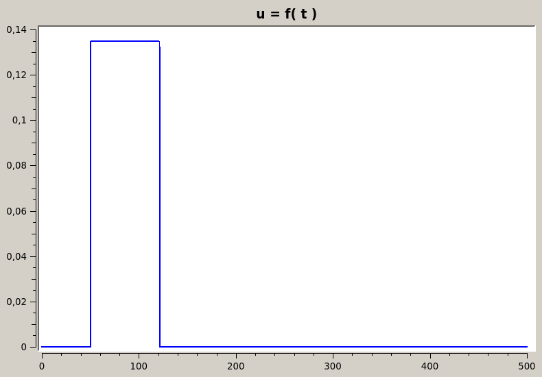
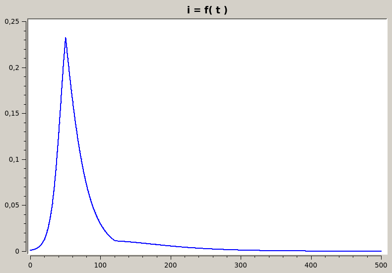
Figure 8: Optimal control and state of infections for $\lambda_{2}=6$

Example 10.2

Our second simulation differs from the first simply because we now impose the ICU constraint with $i_{M}=0.0031$. The viability regions and the corresponding position of the initial point $(s_{0},i_{0})=(0.94,0.001)$ are shown in Figure 6. For $\lambda_{2}\in[0,8]$, the solver converged always to the greedy solution (displayed in the Figure 9). For a greater choice of $\lambda_{2}$ we have not been able to obtain a numerical solution.

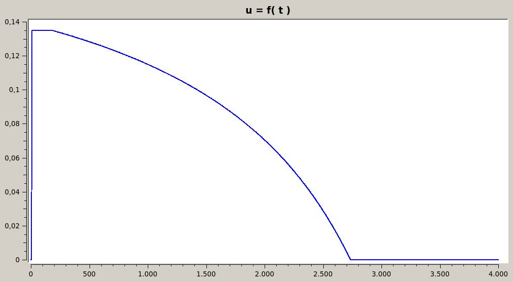
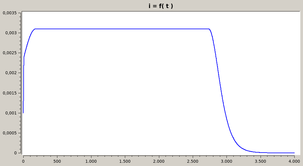
Figure 9: Optimal control and state of infections for $\lambda_{2}\in[0,8]$

Example 10.3 (Italy)

Our last simulation concerns the Covid-19 epidemic state of autumn 2021 in Italy considered in the second part of Example 4.3. The epidemic parameters are $\gamma=0.0714$, $\beta=0.5$, $i_{M}=0.021$, $u_{\max}=0.315$. Computations are done starting from $s_{0}=0.5$ and $i_{0}=0.001$. The viability regions and the corresponding position of the initial point $(s_{0},i_{0})$ are shown in Figure 7. We consider a time horizon of 600 days. For $\lambda_{2}\in[0,19]$ the solver converged always to the greedy solution. From $\lambda_{2}=20$ a second $u_{\max}$ regime starts to appear. The graphs of the optimal control and the corresponding state of infections are displayed in Figure 10 for $\lambda_{2}=30$.

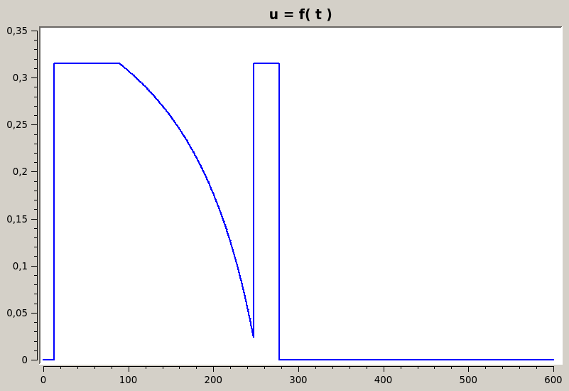
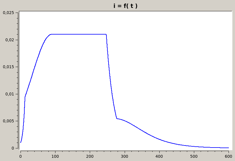
Figure 10: Optimal control and state of infections for $\lambda_{2}=30$

11 Conclusions

We studied the infinite horizon optimal control problem for a SIR epidemic with an ICU contraint. We proved that, starting from an initial epidemic state $(s_{0},i_{0})$ in the viable set, there exists an optimal control of the form

$$u(t)=\begin{cases}0&\mbox{ if }t\in(0,\tau_{0}),\\ {u_{\max}}&\mbox{ if }t\in(\tau_{0},\tau_{1}),\\ \displaystyle\beta-\frac{\gamma}{s(\tau_{2})+\gamma i_{M}(\tau_{2}-t)}&\mbox{ if }t\in(\tau_{1},\tau_{2}),\\[8.61108pt] {u_{\max}}&\mbox{ in }(\tau_{2},\tau_{3}),\\ 0&\mbox{ in }(\tau_{3},\infty),\end{cases}$$

for a suitable choice of times $0\leq\tau_{0}\leq\tau_{1}\leq\tau_{2}\leq\tau_{3}<\infty$. Some numerical simulations have been performed to illustrate this result. Finally, let us emphasize that the problem under consideration in which purely confinement-related costs $\lambda_{1}u$ are completed with social security (convalescence) costs $\lambda_{2}i$ provides a multi strict confinement scenario (illustrated by the presence of the two $u_{\max}$ branches).

References

- [1] F. E. Alvarez, D. Argente, and F. Lippi. A simple planning problem for covid-19 lockdown. Technical report, National Bureau of Economic Research, 2020.
- [2] R. M. Anderson, B. Anderson, and R. M. May. Infectious diseases of humans: dynamics and control. Oxford university press, 1992.
- [3] F. Avram, L. Freddi, and D. Goreac. Corrigendum to “Optimal control of a SIR epidemic with ICU constraints and target objectives”. Appl. Math. Comput., 423:Paper No. 127012, 2, 2022.
- [4] F. Avram, L. Freddi, and D. Goreac. Optimal control of a SIR epidemic with ICU constraints and target objectives. Appl. Math. Comput., 418:Paper No. 126816, 22, 2022.
- [5] H. Behncke. Optimal control of deterministic epidemics. Optimal control applications and methods, 21(6):269–285, 2000.
- [6] H. Bhapkar, P. Mahalle, and N. e. a. Dey. Revisited covid-19 mortality and recovery rates: Are we missing recovery time period? J Med Syst, 44(202), 2020.
- [7] J. Bonnans, Frederic, D. Giorgi, V. Grelard, B. Heymann, S. Maindrault, P. Martinon, O. Tissot, and J. Liu. Bocop – A collection of examples. Technical report, INRIA, 2017.
- [8] J. F. Bonnans. Course on optimal control. Part I: the Pontryagin approach. 2020.
- [9] J. F. Bonnans, C. De La Vega, and X. Dupuis. First-and second-order optimality conditions for optimal control problems of state constrained integral equations. Journal of Optimization Theory and Applications, 159(1):1–40, 2013.
- [10] J. F. Bonnans and C. S. F. de la Vega. Optimal control of state constrained integral equations. Set-Valued and Variational Analysis, 18(3-4):307–326, 2010.
- [11] A. Braides. -convergence for beginners, volume 22 of Oxford Lecture Series in Mathematics and its Applications. Oxford University Press, Oxford, 2002.
- [12] H. Brezis. Functional analysis, Sobolev spaces and partial differential equations. Universitext. Springer, New York, 2011.
- [13] G. Buttazzo. Semicontinuity, relaxation and integral representation in the calculus of variations, volume 207 of Pitman Research Notes in Mathematics Series. Longman Scientific & Technical, Harlow; copublished in the United States with John Wiley & Sons, Inc., New York, 1989.
- [14] G. Dal Maso. An Introduction to -convergence. Birkhäuser, Boston, 1993.
- [15] E. De Giorgi and T. Franzoni. Su un tipo di convergenza variazionale. Atti Accad. Naz. Lincei Rend. Cl. Sci. Fis. Mat. Natur. (8), 58(6):842–850, 1975.
- [16] E. De Giorgi and T. Franzoni. Su un tipo di convergenza variazionale. Rend. Sem. Mat. Brescia, 3:63–101, 1979.
- [17] Decreto-legge 19 maggio 2020, n. 34. Misure urgenti in materia di salute, sostegno al lavoro e all’economia, nonché di politiche sociali connesse all’emergenza epidemiologica da covid-19. (20g00052). https://www.gazzettaufficiale.it/eli/id/2020/05/19/20G00052/sg, 2020. Gazzetta Ufficiale della Repubblica Italiana, n.128 del 19-5-2020 - Suppl. Ordinario n. 21.
- [18] Decreto-legge 23 luglio 2021, n. 105. Misure urgenti per fronteggiare l’emergenza epidemiologica da covid-19 e per l’esercizio in sicurezza di attivita’ sociali ed economiche. (21g00117). https://www.gazzettaufficiale.it/eli/id/2021/07/23/21G00117/sg, 2020. Gazzetta Ufficiale della Repubblica Italiana, Serie Generale n.175 del 23-07-2021.
- [19] I. Fonseca and G. Leoni. Modern methods in the calculus of variations: spaces. Springer Monographs in Mathematics. Springer, New York, 2007.
- [20] L. Freddi. Optimal control of the transmission rate in compartmental epidemics. Math. Control Relat. Fields, 12(1):201–223, 2022.
- [21] L. Freddi, D. Goreac, J. Li, and B. Xu. SIR epidemics with state-dependent costs and ICU constraints: a Hamilton-Jacobi verification argument and dual LP algorithms. Appl. Math. Optim., 86(2):Paper No. 23, 31, 2022.
- [22] G. Guzzetta, F. Riccardo, V. Marziano, P. Poletti, F. Trentini, A. Bella, and et al. Impact of a nationwide lockdown on sars-cov-2 transmissibility, italy. Emerg Infect Dis., 27(1), 2021.
- [23] P. Hajlasz. Change of variables formula under minimal assumptions. Colloq. Math., 64(1):93–101, 1993.
- [24] J. K. Hale. Ordinary differential equations. Robert E. Krieger Publishing Co., Inc., Huntington, N.Y., second edition, 1980.
- [25] E. Hansen and T. Day. Optimal control of epidemics with limited resources. Journal of mathematical biology, 62(3):423–451, 2011.
- [26] H. W. Hethcote. The mathematics of infectious diseases. SIAM review, 42(4):599–653, 2000.
- [27] Istituto Superiore di Sanità. Sorveglianza integrata covid-19 in italia, (aggiornamento 25 marzo 2020). https://www.epicentro.iss.it/coronavirus/bollettino/Infografica_25marzo%20ITA.pdf, 2020.
- [28] W. O. Kermack and A. G. McKendrick. A contribution to the mathematical theory of epidemics. Proceedings of the Royal Society of London. Series A, Containing Papers of a Mathematical and Physical Character, 115(772):700–721, 1927.
- [29] D. I. Ketcheson. Optimal control of an sir epidemic through finite-time non-pharmaceutical intervention. Journal of Mathematical Biology, 83(1):7, Jun 2021.
- [30] T. Kruse and P. Strack. Optimal control of an epidemic through social distancing. 2020.
- [31] Y. Liu and J. Rocklöv. The reproductive number of the Delta variant of SARS-CoV-2 is far higher compared to the ancestral SARS-CoV-2 virus. Journal of Travel Medicine, 28(7), 08 2021. taab124.
- [32] M. Martcheva. An introduction to mathematical epidemiology, volume 61. Springer, 2015.
- [33] L. Miclo, D. Spiro, and J. Weibull. Optimal epidemic suppression under an icu constraint. arXiv preprint arXiv:2005.01327, 2020.
- [34] E. Molina and A. Rapaport. An optimal feedback control that minimizes the epidemic peak in the SIR model under a budget constraint. Automatica J. IFAC, 146:Paper No. 110596, 8, 2022.
- [35] W. Rudin. Principles of mathematical analysis. International Series in Pure and Applied Mathematics. McGraw-Hill Book Co., New York-Auckland-Düsseldorf, third edition, 1976.
- [36] S. Talic, S. Shah, H. Wild, D. Gasevic, A. Maharaj, Z. Ademi, X. Li, W. Xu, I. Mesa-Eguiagaray, J. Rostron, E. Theodoratou, X. Zhang, A. Motee, D. Liew, and D. Ilic. Effectiveness of public health measures in reducing the incidence of covid-19, sars-cov-2 transmission, and covid-19 mortality: systematic review and meta-analysis. BMJ, 375, 2021.
- [37] I. S. Team Commands. Bocop: an open source toolbox for optimal control. http://bocop.org, 2017.