Multi-Linear Pseudo-PageRank for Hypergraph Partitioning

Abstract

Motivated by the PageRank model for graph partitioning, we develop an extension of PageRank for partitioning uniform hypergraphs. Starting from adjacency tensors of uniform hypergraphs, we establish the multi-linear pseudo-PageRank (MLPPR) model, which is formulated as a multi-linear system with nonnegative constraints. The coefficient tensor of MLPPR is a kind of Laplacian tensors of uniform hypergraphs, which are almost as sparse as adjacency tensors since no dangling corrections are incorporated. Furthermore, all frontal slices of the coefficient tensor of MLPPR are M-matrices. Theoretically, MLPPR has a solution, which is unique under mild conditions. An error bound of the MLPPR solution is analyzed when the Laplacian tensor is slightly perturbed. Computationally, by exploiting the structural Laplacian tensor, we propose a tensor splitting algorithm, which converges linearly to a solution of MLPPR. Finally, numerical experiments illustrate that MLPPR is powerful and effective for hypergraph partitioning problems.

MSC Classification]05C90, 15A69, 65C40, 65H10

1 Introduction

PageRank is the first and best-known method developed by Google to evaluate the importance of web-pages via their inherent graph and network structures BP'98 ; BL'06 . There are three advantages of PageRank: existence and uniqueness of the PageRank solution, fast algorithms for finding the PageRank solution, and a built-in regularization Gl'15 . Thus, PageRank and its generalizations have been extensively used in network analysis, image sciences, sports, biology, chemistry, mathematical systems, and so on Gl'15 ; LM'06 . Hypergraphs have the capability of modeling connections among objects according to their inherent multiwise similarity and affinity. Recently, higher-order organization of complex networks at the level of small network subgraphs becomes an active research area BGL16 ; BGL'17 ; KW06 ; RELWL14 . The set of small network subgraphs with common connectivity patterns in a complex network could be modeled by a uniform hypergraph. A natural question is how can we generalize the PageRank idea from graphs to uniform hypergraphs.

PageRank was originally interpreted as a special Markov chain LM'06 , where the transition probability matrix is a columnwise-stochastic matrix. Many algorithms, e.g., power methods, were employed to find the dominant eigenvector of the PageRank eigensystem IS08 . Alternatively, PageRank could be represented as a linear system with an M-matrix, which has favorable theoretical character F15 and good numerical performance LM06 . In the context of PageRank for partitioning a graph, although a Laplacian matrix of the graph is an M-matrix, an adjacency matrix of the graph is not necessarily columnwise-stochastic, when the graph has dangling vertices Ch'05 . Some traditional approaches ACL'07 ; ACL'08 ; Gl'15 ; LM06 incorporated a rank-one correction into a graph adjacency matrix and thus produced a columnwise-stochastic matrix. Using this columnwise-stochastic matrix, PageRank generates the stochastic solution. However, the rank-one correction of the graph adjacency matrix has no graphic meaning. Alternatively, following the framework of M-linear systems, Gleich Gl'15 used the graph Laplacian matrix, which is only columnwise-substochastic, to construct a pseudo-PageRank model. The pseudo-PageRank model outputs the nonnegative solution, which is normalized to obtain the stochastic solution if necessary. Pseudo-PageRank comes from a graph Laplacian matrix directly and is more suitable for practical applications LM06 ; Gl'15 . Moreover, the pseudo-PageRank model is potentially true of the multi-linear cases. This is the primary motivation of this paper.

To explore higher-order extensions of classical Markov chain and PageRank for large-scale practical problems, on one hand, Li and Ng LN'14 used a rank-one array to approximate the limiting probability distribution array of a higher-order Markov chain. The vector for generating the rank-one array is called the limiting probability distribution vector of the higher-order Markov chain. On the other hand, Benson et al. BGL'17 studied the spacey random surfer, which remembers bits and pieces of history and is influenced by this information. Motivated by the spacey random surfer, Gleich et al. GLY'15 developed the multi-linear PageRank (MPR) model, of which the stochastic solution is called a multi-linear PageRank vector. Indeed, the multi-linear PageRank vector could be viewed as a limiting probability distribution vector of a special higher-order Markov chain.

According to the Brouwer fixed-point theorem, a stochastic solution of MPR always exists GLY'15 . The uniqueness of MPR solutions and related problems are more complicated than that of the classical PageRank. Many researchers gave various sufficient conditions CZ'13 ; FT'20 ; GLY'15 ; LLNV'17 ; LLVX'20 ; LN'14 . Dynamical systems of MPR were studied in BGL'17 . The perturbation analysis and error bounds of MPR solutions were presented in LCN'13 ; LLVX'20 . The ergodicity coefficient to a stochastic tensor was addressed in FT'20 . Interestingly, Benson B'19 studied three eigenvector centralities corresponding to tensors arising from hypergraphs. Tensor eigenvectors determine MPR vectors of these stochastic processes and capture some important higher-order network substructures BGL'15 ; BGL'17 .

For solving MPR and associated higher-order Markon chains, Li and Ng LN'14 proposed a fixed-point iteration, which converges linearly when a sufficient condition for uniqueness holds. Gleich et al. GLY'15 studied five numerical methods: a fixed-point iteration, a shifted fixed-point iteration, a nonlinear inner-outer iteration, an inverse iteration, and a Newton iteration. Meini and Poloni MP'18 solved a sequence of PageRank subproblems for Perron vectors to approximate the MPR solution. Furthermore, Huang and Wu HW'21 analyzed this Perron-based algorithm. Liu et al. LLV'19 designed and analyzed several relaxation algorithms for solving MPR. Cipolla et al. CRT'20 introduced extrapolation-based accelerations for a shifted fixed-point method and an inner-outer iteration. Hence, it is an active research area to compute MPR vectors arising from practical problems.

1.1 Contributions

In the process of extending the pseudo-PageRank method from graphs to uniform hypergraphs, the contributions are given as follows.

• Using a Laplacian tensor of a uniform hypergraph directly without any dangling corrections, we propose the multi-linear pseudo-PageRank (MLPPR) model for a uniform hypergraph, which is a multi-linear system with nonnegative constraints. Every frontal slice of the coefficient tensor of MLPPR is an M-matrix. Comparing MLPPR with MPR, MLPPR admits a columuwise-substochastic tensor with dangling column fibers, while MPR rejects any dangling column fibers.

• The theoretical framework of the proposed model is established. The existence and uniqueness of the solution of MLPPR are discussed. The perturbation bound of the MLPPR solution is also presented.

• According to the structure of the tensor in MLPPR, we design a tensor splitting algorithm for finding a solution of MLPPR. Under suitable conditions, the propose algorithm converges linearly to a solution of MLPPR.

• As applications, we employ MLPPR to conduct hypergraph partitioning problems. For the problem of subspace clustering, we illustrate that MLPPR finds vertices of the target cluster more accurately when compared with some existing methods. For network analysis, directed 3-cycles in real-world networks are carefully selected for constructing edges of $3$-uniform hypergraphs. For such hypergraphs, numerical experiments illustrate that the new method is effective and efficient.

1.2 Organization

The outline of this paper is drawn as follows. Section 2 gives preliminary on tensors and graph-based PageRank. Hypergraphs and MLPPR are introduced in Section 3 and theoretical results on MLPPR are presented here. In Section 4, a tensor splitting algorithm for solving MLPPR is customized and analyzed. Applications in hypergraph partitioning problems are reported in Sections 5. Finally, we conclude this paper in Section 6.

2 Preliminary

Before starting, we introduce our notations and definitions. We denote scalars, vectors, matrices, and tensors by lower case ($a$), bold lower case ($\mathbf{a}$), capital case ($A$), and calligraphic script ($\mathcal{A}$), respectively. Let $\mathbb{R}^{[k,n]}$ be the space of $k$th order $n$ dimensional real tensors and let $\mathbb{R}^{[k,n]}_{+}$ be the set of nonnegative tensors in $\mathbb{R}^{[k,n]}$. A tensor $\mathcal{P}\in\mathbb{R}^{[k,n]}$ is called semi-symmetric if all of its elements $p_{i_{1}i_{2}\dots i_{k}}$ are invariant for any permutations of the second to the last indices $i_{2},\dots,i_{k}$.

For $s\in\{1,\dots,k\}$, the $s$-mode product of $\mathcal{P}\in\mathbb{R}^{[k,n]}$ and $\mathbf{x}\in\mathbb{R}^{n}$ produces a $(k-1)$th order $n$ dimensional tensor $\mathcal{P}\bar{\times}_{s}\mathbf{x}$ of which elements are defined by

$$[\mathcal{P}\bar{\times}_{s}\mathbf{x}]_{i_{1}\dots i_{s-1}i_{s+1}\dots i_{k}}:=\sum_{i_{s}=1}^{n}p_{i_{1}\dots i_{s}\dots i_{k}}x_{i_{s}}.$$

For convenience, we define $\mathcal{P}\mathbf{x}^{k-s}:=\mathcal{P}\bar{\times}_{s+1}\mathbf{x}\cdots\bar{\times}_{k}\mathbf{x}$. Particularly, $\mathcal{P}\mathbf{x}^{k-1}$ and $\mathcal{P}\mathbf{x}^{k-2}$ are a vector and a matrix, respectively. For a $k$th order tensor $\mathcal{X}$ and an $\ell$th order tensor $\mathcal{Y}$, the tensor outer product $\mathcal{X}\circ\mathcal{Y}$ is a $(k+\ell)$th order tensor, of which elements are

$$[\mathcal{X}\circ\mathcal{Y}]_{i_{1}\dots i_{k}i_{k+1}\dots i_{k+\ell}}=[\mathcal{X}]_{i_{1}\dots i_{k}}[\mathcal{Y}]_{i_{k+1}\dots i_{k+\ell}}.$$

Particularly, when $k=\ell=1$, the outer product of two vectors $\mathbf{x}$ and $\mathbf{y}$ is a rank-one matrix $\mathbf{x}\circ\mathbf{y}=\mathbf{x}\mathbf{y}^{T}$.

Let $\mathbf{e}_{n}:=(1,1,\dots,1)^{T}\in\mathbb{R}^{n}$ be an all-one vector. For convenience, we denote $\mathbf{e}=\mathbf{e}_{n}$. If $\mathbf{v}\in\mathbb{R}^{n}_{+}$ satisfies $\mathbf{e}^{T}\mathbf{v}=1$, $\mathbf{v}$ is called a stochastic vector. The $1$-mode unfolding of a tensor $\mathcal{P}\in\mathbb{R}^{[k,n]}$ is an $n$-by-$n^{k-1}$ matrix $\mathbf{R}(\mathcal{P})$ of which elements are

$$[\mathbf{R}(\mathcal{P})]_{i\ell}:=p_{ij_{2}j_{3}\dots j_{k}},\quad\text{ where }\quad\ell=j_{2}+(j_{3}-1)n+\cdots+(j_{k}-1)n^{k-2}.$$

Each column of $\mathbf{R}(\mathcal{P})$ is called a mode-1 (column) fiber of the tensor $\mathcal{P}$. If all of column fibers of $\mathcal{P}$ are stochastic, i.e., $\mathcal{P}\in\mathbb{R}^{[k,n]}_{+}$ and $\mathbf{e}^{T}\mathbf{R}(\mathcal{P})=\mathbf{e}^{T}_{n^{k-1}}$, $\mathcal{P}$ is called a columnwise-stochastic tensor. $\mathcal{P}$ is said to be a columnwise-substochastic tensor if $\mathcal{P}\in\mathbb{R}^{[k,n]}_{+}$ and $\mathbf{e}^{T}\mathbf{R}(\mathcal{P})\leq\mathbf{e}^{T}_{n^{k-1}}$. Obviously, a columnwise-stochastic tensor is columnwise-substochastic and not conversely. In the remainder of this paper, a fiber refers to a mode-1 (column) fiber. For given indices $i_{3},\dots,i_{k}$, an $n\times n$ matrix $(p_{iji_{3}\dots i_{k}})_{i,j=1,\dots,n}$ is called a frontal slice of a tensor $\mathcal{P}\in\mathbb{R}^{[k,n]}$.

Next, we briefly review PageRank for directed graphs. A directed graph $G=(V,\vec{E},\mathbf{w})$ contains a vertex set $V:=\{1,2,\dots,n\}$, an arc set $\vec{E}:=\{\vec{e}_{1},\vec{e}_{2},\dots,\vec{e}_{m}\}$, and a weight vector $\mathbf{w}\in\mathbb{R}^{m}_{+}$. A component $w_{\ell}$ of $\mathbf{w}$ stands for the weight of an arc $\vec{e}_{\ell}$ for $\ell=1,\dots,m$. An arc $\vec{e}=(j,i)\in\vec{E}$ means an directed edge $(j,i)$ from vertex $j$ to vertex $i$, where $j$ has an out-neighbor $i$ and $i$ has an in-neighbor $j$. The out-degree $d^{\mathrm{out}}_{j}$ of $j\in V$ is defined by the sum of weights of arcs that depart from $j$:

$$d^{\mathrm{out}}_{j}:=\sum_{i:(j,i)=\vec{e}_{\ell}\in\vec{E}}w_{\ell}\geq 0.$$

If $d^{\mathrm{out}}_{j}=0$, vertex $j$ is called a dangling vertex. Let the out-degree vector be $\mathbf{d}:=(d^{\mathrm{out}}_{j})\in\mathbb{R}^{n}_{+}$. The adjacency matrix $A=[a_{ij}]\in\mathbb{R}^{n\times n}$ of $G$ is defined with elements

$$a_{ij}:=\left\{\begin{aligned} &w_{\ell},&&\text{ if }(j,i)=\vec{e}_{\ell}\in\vec{E},\\ &0,&&\text{ otherwise.}\end{aligned}\right.$$

Clearly, it holds that $\mathbf{d}^{T}=\mathbf{e}^{T}A$. Vertex $j\in V$ is dangling if and only if the $j$th column of the adjacency matrix $A$ is a dangling (zero) vector.

Let us consider the random walk (stochastic process) $\{X(t):t=0,1,2,\dots\}$ on the vertex set $V=\{1,2,\dots,n\}$ of a directed graph $G$. The random walk takes a step according to the transition probability (columnwise-stochastic) matrix $P=(p_{ij})\in\mathbb{R}^{n\times n}_{+}$ with probability $\alpha\in[0,1)$ and jumps randomly to a fixed distribution $\mathbf{v}=(v_{i})\in\mathbb{R}^{n}_{+}$ with probability $1-\alpha$, i.e.,

$$\mathrm{Prob}\{X(t+1)=i\mid X(t)=j\}=\alpha p_{ij}+(1-\alpha)v_{i},$$ (1)

where $p_{ij}$ denotes the probability of a walk from vertex $j$ to vertex $i$. Here, $p_{ij}>0$ if and only if $(j,i)$ is an arc of $G$. If the out-degree vector $\mathbf{d}$ is positive, the normalized adjacency matrix $AD^{+}$ of $G$ is columnwise-stochastic, where $D:=\mathrm{diag}(\mathbf{d})$ and $(\cdot)^{+}$ stands for the Moore-Penrose pseudo-inverse. However, when the graph contains dangling vertices, the normalized adjacency matrix $AD^{+}$ is columnwise-substochastic but not columnwise-stochastic. Researchers Gl'15 ; LM06 incorporated a rank-one correction (named a dangling correction) into the columnwise-substochastic matrix to produce a columnwise-stochastic matrix:

$$P=AD^{+}+\mathbf{u}\mathbf{c}^{T},$$

where $\mathbf{u}\in\mathbb{R}^{n}$ is a stochastic vector, $\mathbf{c}^{T}:=\mathbf{e}^{T}-\mathbf{e}^{T}AD^{+}$ is an indicator vector of dangling columns of $A$ and thus $\mathbf{c}\in\{0,1\}^{n}$ is an indicator vector of dangling vertices in $V$. Here, $c_{j}=1$ if the $j$th column of $A$ is a zero vector and $j\in V$ is a dangling vertex, $c_{j}=0$ otherwise.

Let a stochastic vector $\mathbf{x}$ be a limiting probability distribution of the random walk $\{X(t)\}$. The random walk (1) could be represented as a classical PageRank:

$$\mathbf{x}=\alpha P\mathbf{x}+(1-\alpha)\mathbf{v},\quad\mathbf{e}^{T}\mathbf{x}=1,\quad\mathbf{x}\in\mathbb{R}^{n}_{+}.$$ (2)

It is well-known that the solution $\mathbf{x}$ of PageRank (2) could be interpreted as the Perron vector (the eigenvector corresponding to the dominant eigenvalue) of a nonnegative matrix, $(\alpha P+(1-\alpha)\mathbf{v}\mathbf{e}^{T})\mathbf{x}=\mathbf{x}$, or the solution of a linear system with its coefficient matrix being an M-matrix, $(I-\alpha P)\mathbf{x}=(1-\alpha)\mathbf{v}$, where $I\in\mathbb{R}^{n\times n}$ is the identity matrix. The linear system $(I-\alpha P)\mathbf{x}=(1-\alpha)\mathbf{v}$ with $\mathbf{u}=\mathbf{v}$ and $P=AD^{+}+\mathbf{u}\mathbf{c}^{T}$ for the graph PageRank could be simplified by finding the solution $\mathbf{y}\in\mathbb{R}^{n}_{+}$ of another structural linear system

$$(I-\alpha AD^{+})\mathbf{y}=\mathbf{v}$$ (3)

and then normalizing solution $\mathbf{y}$ to obtain a stochastic vector $\mathbf{x}=\mathbf{y}/(\mathbf{e}^{T}\mathbf{y})$ Gl'15 . In fact, the system (3) is called a pseudo-PageRank problem. The coefficient matrix $I-\alpha AD^{+}$ is both an M-matrix and a Laplacian matrix of the graph YCO'21 , enjoying good properties from linear algebra and graph theory. It is interesting to note that the pseudo-PageRank model doesn’t need to do any dangling corrections. Indeed, dangling cases are inevitable for hypergraphs.

3 Hypergraph and Multi-linear pseudo-PageRank

Spectral hypergraph theory made great progress in the past decade BP'13 ; CD'12 ; QL17book ; GCH22 . Let $G=(V,E,\mathbf{w})$ be a weighted undirected $k$-uniform hypergraph, where $V:=\{1,2,\dots,n\}$ is the vertex set, $E:=\{e_{j}\subseteq V:~{}\lvert e_{j}\rvert=k\text{ for }j=1,2,\dots,m\}$ is the edge set, and $\mathbf{w}=(w_{j})\in\mathbb{R}^{m}_{+}$ is a positive vector whose component $w_{j}$ denotes the weight of an edge $e_{j}\in E$. Here, $\lvert\cdot\rvert$ means the cardinality of a set. Cooper and Dutle CD'12 defined adjacency tensors of uniform hypergraphs.

Definition 3.1 (CD'12 ).

Let $G=(V,E,\mathbf{w})$ be a weighted undirected $k$-uniform hypergraph with $n$ vertices. An adjacency tensor $\mathcal{A}=(a_{i_{1}\dots i_{k}})\in\mathbb{R}^{[k,n]}_{+}$ of $G$ is a symmetric and nonnegative tensor of which elements are

$$a_{i_{1}\dots i_{k}}:=\left\{\begin{aligned} &\frac{w_{j}}{(k-1)!},&&\text{ if }\{i_{1},\dots,i_{k}\}=e_{j}\in E,\\ &0,&&\text{ otherwise. }\end{aligned}\right.$$ (4)

Our MLPPR model could be applied in a weighted directed $k$-uniform hypergraph $G=(V,\vec{E},\mathbf{w})$ with a vertex set $V=\{1,2,\dots,n\}$, an arc set $\vec{E}:=\{\vec{e}_{1},\vec{e}_{2},\dots,\vec{e}_{m}\}$, and weights of arcs $\mathbf{w}\in\mathbb{R}^{m}_{+}$. An arc $\vec{e}_{j}\in\vec{E}$ is an ordered subset $\vec{e}_{j}:=(i_{j,1},i_{j,2},\dots,$ $i_{j,k})$ of $V$ for $j=1,2,\dots,m$. Here, vertices $i_{j,1},\dots,i_{j,k-1}$ are called tails of the arc $\vec{e}_{j}$ and the order among them are irrelevant. The last vertex $i_{j,k}$ is coined the head of the arc $\vec{e}_{j}$. Each arc $\vec{e}_{j}$ has a positive weight $w_{j}$ for $j=1,2,\dots,m$. Similarly, we define an adjacency tensor for the directed $k$-uniform hypergraph $G$ as follows.

Definition 3.2.

Let $G=(V,\vec{E},\mathbf{w})$ be a weighted directed $k$-uniform hypergraph with $n$ vertices. An adjacency tensor $\mathcal{A}=(a_{i_{1}\dots i_{k}})\in\mathbb{R}^{[k,n]}_{+}$ of $G$ is a nonnegative tensor of which elements are

$$a_{i_{1}\dots i_{k}}:=\left\{\begin{aligned} &\frac{w_{j}}{(k-1)!},&&\text{ if }(\sigma(i_{2},\dots,i_{k}),i_{1})=\vec{e}_{j}\in\vec{E},\\ &0,&&\text{ otherwise, }\end{aligned}\right.$$ (5)

where $\sigma(i_{2},\dots,i_{k})$ denotes any permutation of indices $i_{2},\dots,i_{k}$.

Clearly, an adjacency tensor $\mathcal{A}$ of $G$ is semi-symmetric. We note that an edge $\{i_{1},\dots,i_{k}\}$ of an undirected hypergraph could be viewed as $k$ varieties of arcs: $(\sigma(i_{1},\dots,i_{k-1}),i_{k}),(\sigma(i_{k},i_{1},\dots,i_{k-2}),i_{k-1}),\dots,(\sigma(i_{2},\dots,i_{k}),i_{1})$ of a directed hypergraph. In this sense, Definitions 3.2 and 3.1 are consistent.

Next, we consider dangling fibers of an adjacency tensor arising from a uniform hypergraph. There are two kinds of dangling cases. (i) The structural dangling fibers are due to the definition of adjacency tensors of uniform hypergraphs. For example, since the 3-uniform hypergraph does not have edges/arcs with repeating vertices, elements $a_{ijj}$ of the associated adjacency tensor $\mathcal{A}$ are zeros for all $i$ and $j$. Hence, there are structural dangling fibers in adjacency tensors of any $k$-uniform hypergraphs with $k\geq 3$. We note that a graph has no structural dangling fibers. (ii) The sparse dangling fibers are generated by the sparsity of a certain uniform hypergraph. For a set of tail vertices $\{i_{1},\dots,i_{k-1}\}\subset V$, if there is no head vertex $i_{k}\in V$ such that $(\sigma(i_{1},\dots,i_{k-1}),i_{k})\in\vec{E}$, there exist sparse dangling fibers. Particularly, there are amount of dangling fibers in adjacency tensors of large-scale sparse hypergraphs. A complete hypergraph does not have any sparse dangling fibers but has structural dangling fibers.

Example 3.3.

Let $G=(V,E,\mathbf{w})$ be a $3$-uniform undirected hypergraph with $V=\{1,2,3,4\}$, $E=\{\{1,2,3\},\{2,3,4\}\}$, and $\mathbf{w}=\mathbf{e}_{4}$. By Definition 3.1, the unfolding $\mathbf{R}(\mathcal{A})\in\mathbb{R}^{4\times 16}$ of the adjacency tensor $\mathcal{A}\in\mathbb{R}^{[3,4]}$ of $G$ is written as follows:

$$\bordermatrix{&\text{\scriptsize 11}&\text{\scriptsize 21}&\text{\scriptsize 31}&\text{\scriptsize 41}&\text{\scriptsize 12}&\text{\scriptsize 22}&\text{\scriptsize 32}&\text{\scriptsize 42}&\text{\scriptsize 13}&\text{\scriptsize 23}&\text{\scriptsize 33}&\text{\scriptsize 43}&\text{\scriptsize 14}&\text{\scriptsize 24}&\text{\scriptsize 34}&\text{\scriptsize 44}\cr\text{\scriptsize 1}&&&&&&&\frac{1}{2}&&&\frac{1}{2}&&&&&&\cr\text{\scriptsize 2}&&&\frac{1}{2}&&&&&&\frac{1}{2}&&&\frac{1}{2}&&&\frac{1}{2}&\cr\text{\scriptsize 3}&&\frac{1}{2}&&&\frac{1}{2}&&&\frac{1}{2}&&&&&&\frac{1}{2}&&\cr\text{\scriptsize 4}&&&&&&&\frac{1}{2}&&&\frac{1}{2}&&&&&&\cr}.$$

Obviously, columns $11$, $22$, $33$, and $44$ are structural dangling fibers. Columns $41$ and $14$ are sparse dangling fibers.

To get rid of these dangling fibers that lead to a gap between Laplacian tensors of uniform hypergraphs and columnwise-stochastic tensors for higher-order extensions of PageRank, we are going to develop a novel MLPPR model. Following the spirit of the pseudo-PageRank model for graphs, we normalize all nonzero fibers of the adjacency tensor $\mathcal{A}$ of a uniform hypergraph $G$ to produce a columnwise-substochastic tensor $\bar{\mathcal{P}}=(\bar{p}_{i_{1}\dots i_{k}})\in\mathbb{R}^{[k,n]}_{+}$, of which elements are defined by

$$\bar{p}_{i_{1}\dots i_{k}}=\left\{\begin{aligned} &\frac{a_{i_{1}\dots i_{k}}}{\sum\limits_{\ell=1}^{n}a_{\ell i_{2}\dots i_{k}}},&&\text{ if }\sum_{\ell=1}^{n}a_{\ell i_{2}\dots i_{k}}>0,\\ &0,&&\text{ otherwise.}\end{aligned}\right.$$ (6)

That is to say, we have $\mathbf{R}(\bar{\mathcal{P}})=\mathbf{R}(\mathcal{A})D^{+}\in\mathbb{R}^{n\times n^{k-1}}_{+}$, where $D:=\mathrm{diag}(\mathbf{e}^{T}\mathbf{R}(\mathcal{A}))$. Both an adjacency tensor $\mathcal{A}$ and its normalization $\bar{\mathcal{P}}$ are nonnegative tensors, which have interesting theoretical results LN15 .

As an analogue of the Laplacian matrix of a graph YCO'21 , we call

$$I\circ\mathbf{e}^{\circ(k-2)}-\alpha\bar{\mathcal{P}}\in\mathbb{R}^{[k,n]}$$

a Laplacian tensor of a $k$-uniform hypergraph $G$ with $n$ vertices, where $\alpha\in[0,1)$ is a probability and $\mathbf{e}^{\circ(k-2)}$ is the outer produce of $k-2$ copies of $\mathbf{e}$. Obviously, each frontal slice of this Laplacian tensor is an M-matrix. Now, we are ready to present the multi-linear pseudo-PageRank model.

Definition 3.4 (MLPPR).

Let $\bar{\mathcal{P}}$ be a columnwise-substochastic tensor, i.e., $\bar{\mathcal{P}}\in\mathbb{R}^{[k,n]}_{+}$ and $\mathbf{e}^{T}\mathbf{R}(\bar{\mathcal{P}})\leq\mathbf{e}^{T}_{n^{k-1}}$. Let $\mathbf{v}\in\mathbb{R}^{n}$ be a stochastic vector and let $\alpha\in[0,1)$ be a probability. Then MLPPR is to find a nonnegative solution $\mathbf{y}\in\mathbb{R}^{n}_{+}$ of the following multi-linear system

$$\left(I\circ\mathbf{e}^{\circ(k-2)}-\alpha\bar{\mathcal{P}}\right)\mathbf{y}^{k-1}=\mathbf{v}.$$ (7)

The normalized $\mathbf{y}$, i.e., $\mathbf{y}/(\mathbf{y}^{T}\mathbf{e})$, is called an MLPPR vector.

Next, we show some properties of the multi-linear system of MLPPR.

Lemma 3.5.

If the MLPPR system (7) has a nonnegative solution $\mathbf{y}_{*}$, then $\mathbf{y}_{*}$ belongs to a bounded, closed and convex set:

$$\Delta:=\{\mathbf{y}\in\mathbb{R}^{n}_{+}:\mathbf{y}^{T}\mathbf{e}\leq\varrho\},$$ (8)

where $\varrho:=(1-\alpha)^{-\frac{1}{k-1}}$.

Proof: Since $\bar{\mathcal{P}}$ is columnwise-substochastic, by taking inner products between $\mathbf{e}$ and both sides of (7), we have

$$1=\mathbf{e}^{T}\mathbf{v}=(\mathbf{e}^{T}\mathbf{y}_{*})^{k-1}-\alpha\mathbf{e}^{T}(\bar{\mathcal{P}}\mathbf{y}_{*}^{k-1})\geq(1-\alpha)(\mathbf{e}^{T}\mathbf{y}_{*})^{k-1},$$ (9)

which means that $\mathbf{y}_{*}$ satisfies $\mathbf{e}^{T}\mathbf{y}_{*}\leq(1-\alpha)^{-\frac{1}{k-1}}=\varrho$. Hence, $\mathbf{y}_{*}\in\Delta$. It is straightforward to see that $\Delta$ is a bounded, closed and convex set.

Lemma 3.6.

Let $\mathbf{y}_{*}\in\Delta$. Then $\mathbf{y}_{*}$ solves the MLPPR system (7) if and only if $\mathbf{y}_{*}$ is a fixed point of the continuous map

$$\Phi(\mathbf{y}):=\left(1+\alpha\mathbf{e}^{T}(\bar{\mathcal{P}}\mathbf{y}^{k-1})\right)^{-\frac{k-2}{k-1}}(\mathbf{v}+\alpha\bar{\mathcal{P}}\mathbf{y}^{k-1}).$$ (10)

Proof: On one hand, assume that $\mathbf{y}_{*}$ solves MLPPR. From (9), we say

$$\mathbf{e}^{T}\mathbf{y}_{*}=\left(1+\alpha\mathbf{e}^{T}(\bar{\mathcal{P}}\mathbf{y}_{*}^{k-1})\right)^{\frac{1}{k-1}}.$$

Then the MLPPR system (7) could be represented as

$$\mathbf{y}_{*}=(\mathbf{e}^{T}\mathbf{y}_{*})^{-(k-2)}(\mathbf{v}+\alpha\bar{\mathcal{P}}\mathbf{y}_{*}^{k-1})=\left(1+\alpha\mathbf{e}^{T}(\bar{\mathcal{P}}\mathbf{y}_{*}^{k-1})\right)^{-\frac{k-2}{k-1}}(\mathbf{v}+\alpha\bar{\mathcal{P}}\mathbf{y}_{*}^{k-1}).$$

That is to say, $\mathbf{y}_{*}$ is a fixed point of $\Phi$.

On the other hand, From $\mathbf{y}_{*}=\Phi(\mathbf{y}_{*})$ we can derive

$$\mathbf{e}^{T}\mathbf{y}_{*}=\mathbf{e}^{T}\Phi(\mathbf{y}_{*})=\left(1+\alpha\mathbf{e}^{T}(\bar{\mathcal{P}}\mathbf{y}_{*}^{k-1})\right)^{\frac{1}{k-1}}.$$

Then the equality (10) reduces to

$$\mathbf{y}_{*}=(\mathbf{e}^{T}\mathbf{y}_{*})^{-(k-2)}(\mathbf{v}+\alpha\bar{\mathcal{P}}\mathbf{y}_{*}^{k-1}),$$

which is equivalent to MLPPR (7).

The following theorem reveals the existence of nonnegative solutions of MLPPR.

Theorem 3.7.

Let $\bar{\mathcal{P}}$, $\mathbf{v}$, and $\alpha$ be defined as in Definition 3.4. Then the MLPPR system (7) has at least one nonzero solution $\mathbf{y}_{*}\in\mathbb{R}^{n}_{+}$.

Proof: At the beginning, we prove that $\Phi$ maps $\Delta$ into itself, where $\Delta$ and $\Phi$ are defined as in Lemmas 3.5 and 3.6, respectively. Let $\mathbf{y}\in\Delta$. Obviously, $\Phi(\mathbf{y})\in\mathbb{R}^{n}_{+}$. By taking an inner product between $\mathbf{e}$ and $\Phi(\mathbf{y})$, we have

$$\mathbf{e}^{T}\Phi(\mathbf{y}) = \left(1+\alpha\mathbf{e}^{T}(\bar{\mathcal{P}}\mathbf{y}^{k-1})\right)^{\frac{1}{k-1}}$$

$$\leq \left(1+\alpha(\mathbf{e}^{T}\mathbf{y})^{k-1}\right)^{\frac{1}{k-1}}$$

$$\leq \left(1+\alpha(1-\alpha)^{-1}\right)^{\frac{1}{k-1}}$$

$$= \varrho,$$

where the first inequality holds because $\bar{\mathcal{P}}$ is columnwise-substochastic. Hence, the continuous function $\Phi$ maps the compact and convex set $\Delta$ into itself.

According to the Brouwer fixed point theorem, there exists $\mathbf{y}_{*}\in\Delta$ such that $\Phi(\mathbf{y}_{*})=\mathbf{y}_{*}$. By Lemma 3.6, $\mathbf{y}_{*}$ is also a nonnegative solution of MLPPR.

Corollary 3.8.

If $\mathbf{v}$ is a positive (stochastic) vector, then a nonnegative solution $\mathbf{y}_{*}=\Phi(\mathbf{y}_{*})$ of MLPPR is also positive.

On the uniqueness of MLPPR solution, we have theoretical results under some conditions. To move on, the following two lemmas are helpful.

Lemma 3.9.

Let $\otimes$ denote the Kronecker product. Define

$$\mathbf{x}^{\otimes(k-1)}:=\underbrace{\mathbf{x}\otimes\mathbf{x}\otimes\cdots\otimes\mathbf{x}}_{k-1\text{ copies of }\mathbf{x}}.$$

For any $\mathbf{x},\mathbf{y}\in\Delta$, we have

$$\|\mathbf{x}^{\otimes(k-1)}-\mathbf{y}^{\otimes(k-1)}\|_{1}\leq(k-1)(1-\alpha)^{-\frac{k-2}{k-1}}\|\mathbf{x}-\mathbf{y}\|_{1}.$$

Proof: By direct calculations with (8), we have

$$\|\mathbf{x}^{\otimes(k-1)}-\mathbf{y}^{\otimes(k-1)}\|_{1}$$

$$= \|(\mathbf{x}-\mathbf{y})\otimes\mathbf{x}^{\otimes(k-2)}+\mathbf{y}\otimes(\mathbf{x}-\mathbf{y})\otimes\mathbf{x}^{\otimes(k-3)}+\cdots+\mathbf{y}^{\otimes(k-2)}\otimes(\mathbf{x}-\mathbf{y})\|_{1}$$

$$\leq \|\mathbf{x}-\mathbf{y}\|_{1}(\mathbf{e}^{T}\mathbf{x})^{k-2}+(\mathbf{e}^{T}\mathbf{y})\|\mathbf{x}-\mathbf{y}\|_{1}(\mathbf{e}^{T}\mathbf{x})^{k-3}+\cdots+(\mathbf{e}^{T}\mathbf{y})^{k-2}\|\mathbf{x}-\mathbf{y}\|_{1}$$

$$\leq (k-1)(1-\alpha)^{-\frac{k-2}{k-1}}\|\mathbf{x}-\mathbf{y}\|_{1},$$

where the last inequality is valid because $\mathbf{x},\mathbf{y}\in\Delta$.

Lemma 3.10.

Define $\varphi(\mathbf{z}):=(\mathbf{e}^{T}\mathbf{z})^{-\frac{k-2}{k-1}}\mathbf{z}$ for $\mathbf{z}\in\Xi:=\{\mathbf{z}\in\mathbb{R}^{n}_{+}:\mathbf{e}^{T}\mathbf{z}\geq 1\}$. For any $\mathbf{a},\mathbf{b}\in\Xi$, we have

$$\|\varphi(\mathbf{a})-\varphi(\mathbf{b})\|_{1}\leq\frac{2k-3}{k-1}\|\mathbf{a}-\mathbf{b}\|_{1}.$$

Proof: Let $\psi(t):=t^{-\frac{k-2}{k-1}}$ for $t\in[1,\infty)$. Obviously, $\psi(t)$ is a convex and monotonically decreasing function on $[1,\infty)$. When $s\geq t\geq 1$, we have

$$\phi(s)-\phi(t)\leq\phi^{\prime}(s)(s-t)$$ (11)

and

$$s^{-\frac{k-2}{k-1}}\leq t^{-\frac{k-2}{k-1}}\leq 1.$$ (12)

For any $\mathbf{a},\mathbf{b}\in\Xi$, without loss of generality, we suppose $\mathbf{e}^{T}\mathbf{a}\geq\mathbf{e}^{T}\mathbf{b}\geq 1$. Then, we have

$$\|\varphi(\mathbf{a})-\varphi(\mathbf{b})\|_{1} = \left\|(\mathbf{e}^{T}\mathbf{a})^{-\frac{k-2}{k-1}}\mathbf{a}-(\mathbf{e}^{T}\mathbf{b})^{-\frac{k-2}{k-1}}\mathbf{b}\right\|_{1}$$

$$\leq (\mathbf{e}^{T}\mathbf{a})^{-\frac{k-2}{k-1}}\|\mathbf{a}-\mathbf{b}\|_{1}+\left\lvert(\mathbf{e}^{T}\mathbf{a})^{-\frac{k-2}{k-1}}-(\mathbf{e}^{T}\mathbf{b})^{-\frac{k-2}{k-1}}\right\rvert\|\mathbf{b}\|_{1}$$

$$= (\mathbf{e}^{T}\mathbf{a})^{-\frac{k-2}{k-1}}\|\mathbf{a}-\mathbf{b}\|_{1}+\left[(\mathbf{e}^{T}\mathbf{b})^{-\frac{k-2}{k-1}}-(\mathbf{e}^{T}\mathbf{a})^{-\frac{k-2}{k-1}}\right](\mathbf{e}^{T}\mathbf{b})$$

$$\leq (\mathbf{e}^{T}\mathbf{a})^{-\frac{k-2}{k-1}}\|\mathbf{a}-\mathbf{b}\|_{1}-\frac{k-2}{k-1}(\mathbf{e}^{T}\mathbf{b})^{-\frac{k-2}{k-1}-1}(\mathbf{e}^{T}\mathbf{b}-\mathbf{e}^{T}\mathbf{a})(\mathbf{e}^{T}\mathbf{b})$$

$$\leq \|\mathbf{a}-\mathbf{b}\|_{1}+\frac{k-2}{k-1}\mathbf{e}^{T}(\mathbf{a}-\mathbf{b})$$

$$\leq \frac{2k-3}{k-1}\|\mathbf{a}-\mathbf{b}\|_{1},$$

where the second and the third inequalities hold owing to (11) and (12), respectively.

Theorem 3.11.

Let $\bar{\mathcal{P}}$, $\mathbf{v}$, and $\alpha$ be defined as in Definition 3.4. Define

$$\varsigma:=(2k-3)\alpha(1-\alpha)^{-\frac{k-2}{k-1}}.$$ (13)

If $\varsigma<1$, then the map $\Phi:\Delta\to\Delta$ is a contraction map, i.e., $\|\Phi(\mathbf{x})-\Phi(\mathbf{y})\|_{1}\leq\varsigma\|\mathbf{x}-\mathbf{y}\|_{1}$ for all $\mathbf{x},\mathbf{y}\in\Delta$.

Proof: For any $\mathbf{x},\mathbf{y}\in\Delta$, we have $\mathbf{v}+\alpha\bar{\mathcal{P}}\mathbf{x}^{k-1},\mathbf{v}+\alpha\bar{\mathcal{P}}\mathbf{y}^{k-1}\in\Xi$ and

$$\|\Phi(\mathbf{x})-\Phi(\mathbf{y})\|_{1} = \|\varphi(\mathbf{v}+\alpha\bar{\mathcal{P}}\mathbf{x}^{k-1})-\varphi(\mathbf{v}+\alpha\bar{\mathcal{P}}\mathbf{y}^{k-1})\|_{1}$$

$$\leq \frac{2k-3}{k-1}\|\mathbf{v}+\alpha\bar{\mathcal{P}}\mathbf{x}^{k-1}-\mathbf{v}-\alpha\bar{\mathcal{P}}\mathbf{y}^{k-1}\|_{1}$$

$$= \alpha\frac{2k-3}{k-1}\|\mathbf{R}(\bar{\mathcal{P}})(\mathbf{x}^{\otimes(k-1)}-\mathbf{y}^{\otimes(k-1)})\|_{1}$$

$$\leq \alpha\frac{2k-3}{k-1}\|\mathbf{x}^{\otimes(k-1)}-\mathbf{y}^{\otimes(k-1)}\|_{1}$$

$$\leq \alpha\frac{2k-3}{k-1}(k-1)(1-\alpha)^{-\frac{k-2}{k-1}}\|\mathbf{x}-\mathbf{y}\|_{1}$$

$$= \varsigma\|\mathbf{x}-\mathbf{y}\|_{1},$$

where the first and the last inequalities are owing to Lemmas 3.10 and 3.9, respectively. The second inequality holds because $\bar{\mathcal{P}}$ is columnwise-substochastic. Hence, $\Phi$ is a contraction map when $\varsigma<1$.

For the special case of the pseudo-PageRank model for graphs, we know $k=2$. Then the condition $\varsigma<1$ reduces to a trivial condition $\alpha<1$. When $k=3$, the condition $\varsigma<1$ reduces to $\alpha<\frac{\sqrt{37}-1}{18}\approx 0.28$. Furthermore, the uniqueness of MLPPR solution follows this contraction theorem.

Corollary 3.12.

Under conditions of Theorem 3.11, the MLPPR system (7) has a unique nonnegative solution $\mathbf{y}_{*}\in\Delta$.

Whereafter, we will consider how perturbations in the columnwise-substochastic tensor $\bar{\mathcal{P}}$ and the stochastic vector $\mathbf{v}$ affect the MLPPR solution $\mathbf{y}$. Numerical verifications of this theorem will be illustrated in Subsection 5.1.

Theorem 3.13.

Let $\bar{\mathcal{P}}$ and $\bar{\mathcal{P}}_{p}=\bar{\mathcal{P}}+\delta\bar{\mathcal{P}}\in\mathbb{R}^{[k,n]}$ be columnwise-substochastic tensors. Let $\mathbf{v}$ and $\mathbf{v}_{p}=\mathbf{v}+\delta\mathbf{v}\in\mathbb{R}^{n}$ be stochastic vectors. The probability $\alpha$ is chosen such that $\varsigma<1$. Nonnegative vectors $\mathbf{y}\in\Delta$ and $\mathbf{y}_{p}=\mathbf{y}+\delta\mathbf{y}\in\Delta$ solve MLPPR systems

$$\left(I\circ\mathbf{e}^{\circ(k-2)}-\alpha\bar{\mathcal{P}}\right)\mathbf{y}^{k-1}=\mathbf{v}\quad\text{ and }\quad\left(I\circ\mathbf{e}^{\circ(k-2)}-\alpha\bar{\mathcal{P}}_{p}\right)\mathbf{y}_{p}^{k-1}=\mathbf{v}_{p},$$

respectively. Then, we have

$$\|\delta\mathbf{y}\|_{1} \leq \frac{2k-3}{(k-1)(1-\varsigma)}\left(\frac{\alpha}{1-\alpha}\|\mathbf{R}(\delta\bar{\mathcal{P}})\|_{1}+\|\delta\mathbf{v}\|_{1}\right).$$

Proof: According to definition of $\varphi$ in Lemma 3.10, we have

$$\|\delta\mathbf{y}\|_{1}=\|\mathbf{y}_{p}-\mathbf{y}\|_{1}$$

$$= \|\varphi(\mathbf{v}_{p}+\alpha\bar{\mathcal{P}}_{p}\mathbf{y}_{p}^{k-1})-\varphi(\mathbf{v}+\alpha\bar{\mathcal{P}}\mathbf{y}^{k-1})\|_{1}$$

$$\leq \frac{2k-3}{k-1}\|\mathbf{v}_{p}+\alpha\bar{\mathcal{P}}_{p}\mathbf{y}_{p}^{k-1}-\mathbf{v}-\alpha\bar{\mathcal{P}}\mathbf{y}^{k-1}\|_{1}$$

$$= \frac{2k-3}{k-1}\|\alpha(\bar{\mathcal{P}}_{p}-\bar{\mathcal{P}})\mathbf{y}_{p}^{k-1}+\alpha(\bar{\mathcal{P}}\mathbf{y}_{p}^{k-1}-\bar{\mathcal{P}}\mathbf{y}^{k-1})+\delta\mathbf{v}\|_{1}$$

$$\leq \alpha\frac{2k-3}{k-1}\|\mathbf{R}(\delta\bar{\mathcal{P}})\|_{1}\|\mathbf{y}_{p}^{\otimes(k-1)}\|_{1}+\alpha\frac{2k-3}{k-1}\|\mathbf{R}(\bar{\mathcal{P}})\|_{1}\|\mathbf{y}_{p}^{\otimes(k-1)}-\mathbf{y}^{\otimes(k-1)}\|_{1}$$

$${}+\frac{2k-3}{k-1}\|\delta\mathbf{v}\|_{1}$$

$$\leq \alpha\frac{2k-3}{k-1}\|\mathbf{R}(\delta\bar{\mathcal{P}})\|_{1}(\mathbf{e}^{T}\mathbf{y}_{p})^{k-1}+\alpha\frac{2k-3}{k-1}\|\mathbf{y}_{p}^{\otimes(k-1)}-\mathbf{y}^{\otimes(k-1)}\|_{1}+\frac{2k-3}{k-1}\|\delta\mathbf{v}\|_{1}$$

$$\leq \frac{\alpha}{1-\alpha}\frac{2k-3}{k-1}\|\mathbf{R}(\delta\bar{\mathcal{P}})\|_{1}+\alpha(1-\alpha)^{-\frac{k-2}{k-1}}(2k-3)\|\delta\mathbf{y}\|_{1}+\frac{2k-3}{k-1}\|\delta\mathbf{v}\|_{1},$$

where the first inequality is valid by Lemma 3.10 and the last inequality follows from $\mathbf{y}_{d}\in\Delta$ and Lemma 3.9. Hence, we obtain

$$\left(\frac{1}{2k-3}-\alpha(1-\alpha)^{-\frac{k-2}{k-1}}\right)\|\delta\mathbf{y}\|_{1}\leq\frac{1}{k-1}\left(\frac{\alpha}{1-\alpha}\|\mathbf{R}(\delta\bar{\mathcal{P}})\|_{1}+\|\delta\mathbf{v}\|_{1}\right).$$

The proof is completed.

3.1 Relationships between MPR and MLPPR

In the framework of MPR BGL'15 ; GLY'15 , a columnwise-substochastic tensor $\bar{\mathcal{P}}$ used in MLPPR was adjusted to a columnwise-stochastic tensor by performing the following dangling correction:

$$\mathcal{P}:=\bar{\mathcal{P}}+\mathbf{v}\circ\left(\mathbf{e}^{\circ(k-1)}-\bar{\mathcal{P}}\bar{\times}_{1}\mathbf{e}\right)\in\mathbb{R}^{[k,n]}_{+}.$$ (14)

We note that the tensor $\mathbf{e}^{\circ(k-1)}-\bar{\mathcal{P}}\bar{\times}_{1}\mathbf{e}\in\mathbb{R}^{[k-1,n]}$ is dense if $\bar{\mathcal{P}}\bar{\times}_{1}\mathbf{e}$ is sparse. Gleich et al. GLY'15 proposed the MPR model:

$$\mathbf{x}=\alpha\mathcal{P}\mathbf{x}^{k-1}+(1-\alpha)\mathbf{v},\quad\mathbf{x}\in\mathbb{R}^{n}_{+},\quad\mathbf{e}^{T}\mathbf{x}=1,$$ (15)

where $\mathcal{P}\in\mathbb{R}^{[k,n]}$ is a columnwise-stochastic tensor and $\mathbf{v}\in\mathbb{R}^{n}$ is a stochastic vector.

We remark that MPR (15) has a homogeneous form

$$\mathbf{z}(\mathbf{e}^{T}\mathbf{z})^{k-2}=\alpha\mathcal{P}\mathbf{z}^{k-1}+(1-\alpha)\mathbf{v}(\mathbf{e}^{T}\mathbf{z})^{k-1},\quad\mathbf{z}\in\mathbb{R}^{n}_{+}.$$ (16)

If the homogeneous form (16) has a nonzero solution $\mathbf{z}$, there are an infinite number of solutions $\gamma\mathbf{z}$ for all $\gamma>0$. Furthermore, a nonzero vector $\mathbf{z}$ solves the homogeneous form (16) if and only if $\mathbf{z}/(\mathbf{e}^{T}\mathbf{z})$ solves MPR (15).

Next, we discuss relationships between MLPPR, MPR, and the homogeneous MPR when the dangling correction (14) holds.

Lemma 3.14.

Suppose the dangling correction (14) holds. If $\mathbf{x}$ solves MPR (15), then

$$\mathbf{y}:=\left(1-\alpha\mathbf{e}^{T}(\bar{\mathcal{P}}\mathbf{x}^{k-1})\right)^{-\frac{1}{k-1}}\mathbf{x}$$

is a nonnegative solution of MLPPR (7).

Proof: From (15) and (14), we have

$$\mathbf{x} = \alpha\mathcal{P}\mathbf{x}^{k-1}+(1-\alpha)\mathbf{v}$$

$$= \alpha\bar{\mathcal{P}}\mathbf{x}^{k-1}+\alpha\mathbf{v}-\alpha\mathbf{v}\mathbf{e}^{T}(\bar{\mathcal{P}}\mathbf{x}^{k-1})+(1-\alpha)\mathbf{v}$$

$$= \alpha\bar{\mathcal{P}}\mathbf{x}^{k-1}+\left(1-\alpha\mathbf{e}^{T}(\bar{\mathcal{P}}\mathbf{x}^{k-1})\right)\mathbf{v},$$

which implies

$$(I\circ\mathbf{e}^{\circ(k-2)}-\alpha\bar{\mathcal{P}})\mathbf{x}^{k-1}\left(1-\alpha\mathbf{e}^{T}(\bar{\mathcal{P}}\mathbf{x}^{k-1})\right)^{-1}=\mathbf{v}.$$

The proof is completed.

Lemma 3.15.

Suppose the dangling correction (14) holds. If a nonnegative vector $\mathbf{y}$ solves MLPPR (7), then $\mathbf{y}$ is a solution of the homogeneous form of MPR (16).

Proof: By taking inner products between $\mathbf{e}$ and both sides of (7), we get

$$\alpha\mathbf{e}^{T}(\bar{\mathcal{P}}\mathbf{y}^{k-1})=(\mathbf{e}^{T}\mathbf{y})^{k-1}-1.$$

Then, it follows from (7) and (14) that

$$\mathbf{v} = \mathbf{y}(\mathbf{e}^{T}\mathbf{y})^{k-2}-\alpha\bar{\mathcal{P}}\mathbf{y}^{k-1}$$

$$= \mathbf{y}(\mathbf{e}^{T}\mathbf{y})^{k-2}-\alpha\mathcal{P}\mathbf{y}^{k-1}+\alpha\mathbf{v}(\mathbf{e}^{T}\mathbf{y})^{k-1}-\alpha\mathbf{v}\mathbf{e}^{T}(\bar{\mathcal{P}}\mathbf{y}^{k-1})$$

$$= \mathbf{y}(\mathbf{e}^{T}\mathbf{y})^{k-2}-\alpha\mathcal{P}\mathbf{y}^{k-1}+\alpha\mathbf{v}(\mathbf{e}^{T}\mathbf{y})^{k-1}-\mathbf{v}((\mathbf{e}^{T}\mathbf{y})^{k-1}-1)$$

$$= \mathbf{y}(\mathbf{e}^{T}\mathbf{y})^{k-2}-\alpha\mathcal{P}\mathbf{y}^{k-1}-(1-\alpha)\mathbf{v}(\mathbf{e}^{T}\mathbf{y})^{k-1}+\mathbf{v},$$

which implies (16) straightforwardly.

According to Lemmas 3.14 and 3.15, we get the following unexpected but reasonable theorem.

Theorem 3.16.

Let $\bar{\mathcal{P}}$, $\mathbf{v}$, and $\alpha$ be defined as in Definition 3.4. Suppose the dangling correction (14) holds. Then the solution of MPR (15) is unique if and only if the nonnegative solution of MLPPR (7) is unique.

Proof: Suppose that $\mathbf{y}_{1}$ and $\mathbf{y}_{2}$ are nonnegative solutions of MLPPR (7). By Lemma 3.15, $\mathbf{y}_{1}/(\mathbf{e}^{T}\mathbf{y}_{1})$ and $\mathbf{y}_{2}/(\mathbf{e}^{T}\mathbf{y}_{2})$ are solutions of MPR (15). Because MPR has a unique solution, we have

$$\mathbf{y}_{1}/(\mathbf{e}^{T}\mathbf{y}_{1})=\mathbf{y}_{2}/(\mathbf{e}^{T}\mathbf{y}_{2}),$$

which means $\mathbf{y}_{1}=\gamma\mathbf{y}_{2}$ for a positive number $\gamma$.

On the other hand, because $\mathbf{y}_{1}$ and $\mathbf{y}_{2}$ solve MLPPR (7), we have

$$\mathbf{v} = (I\circ\mathbf{e}^{\circ(k-2)}-\alpha\bar{\mathcal{P}})\mathbf{y}_{1}^{k-1}$$

$$= (I\circ\mathbf{e}^{\circ(k-2)}-\alpha\bar{\mathcal{P}})(\gamma\mathbf{y}_{2})^{k-1}$$

$$= \gamma^{k-1}(I\circ\mathbf{e}^{\circ(k-2)}-\alpha\bar{\mathcal{P}})\mathbf{y}_{2}^{k-1}$$

$$= \gamma^{k-1}\mathbf{v}.$$

Hence, the positive number $\gamma$ is subject to $\gamma^{k-1}-1=0$. We say $\gamma=1$ which means $\mathbf{y}_{1}=\mathbf{y}_{2}$.

The converse statement could be verified by using Lemma 3.14 and a similar discussion.

Based on Theorem 3.16 and Theorem 4.3 in GLY'15 , we get a new sufficient condition for preserving the uniqueness of an MLPPR solution.

Corollary 3.17.

MLPPR has a unique nonnegative solution when $\alpha<\frac{1}{k-1}$.

Clearly, Corollary 3.17 is better than Corollary 3.12, since we can infer $\alpha<\frac{1}{k-1}$ from $\varsigma=(2k-3)\alpha(1-\alpha)^{-\frac{k-2}{k-1}}<1$ and not conversely when $k\geq 3$. In the case of $k=2$, $\alpha<\frac{1}{k-1}$ is equivalent to $\varsigma<1$. Additionally, other sufficient conditions for the uniqueness of the MPR solution elaborated in LN'14 ; LLNV'17 ; LLVX'20 are also applied to MLPPR.

Comparing with MLPPR, MPR adjusts all fibers of the columnwise-substochastic tensor to stochastic vectors in advance and then MPR returns a stochastic solution. When applied into uniform hypergraphs, the adjustment in MPR lacks significance of graph theory. In addition, it is a time-consuming process to produce the adjustment for large scale hypergraphs. Our MLPPR utilizes the columnwise-substochastic tensor directly to produce a nonnegative solution, which could easily be normalized to a stochastic vector if necessary. By reversing the order of adjustment/normalization and root-finding of constrained multi-linear systems, we proposed a novel MLPPR model. Moreover, MLPPR gets rid of dangling cases by directly dealing with columnwise-substochastic tensors, which are usually sparser than columnwise-stochastic tensors used in MPR. This sparsity reveals a valuable potential of MLPPR in computation.

4 Tensor splitting algorithm

Inspired by the structure of the coefficient tensor of MLPPR, of which all frontal slices are M-matrices, we propose a tensor splitting iterative algorithm. Starting from $\mathbf{y}_{0}\in\Delta$, we repeatedly find a new iterate $\mathbf{y}_{c+1}$ by solving the following subproblems

$$\left(I\circ\mathbf{e}^{\circ(k-2)}\right)\mathbf{y}_{c+1}^{k-1}=\alpha\bar{\mathcal{P}}\mathbf{y}_{c}^{k-1}+\mathbf{v}$$ (17)

for $c=0,1,2,\dots$. This structural tensor equation has a closed-form solution.

Lemma 4.1.

Let $\mathbf{y}_{c}\in\Delta$. Equation (17) has a closed-form solution:

$$\mathbf{y}_{c+1}=\left(1+\alpha\mathbf{e}^{T}(\bar{\mathcal{P}}\mathbf{y}_{c}^{k-1})\right)^{-\frac{k-2}{k-1}}(\alpha\bar{\mathcal{P}}\mathbf{y}_{c}^{k-1}+\mathbf{v})\in\Delta,$$

which is exactly $\mathbf{y}_{c+1}=\Phi(\mathbf{y}_{c})$, where $\Phi$ is defined in Lemma 3.6.

Proof: It follows from a subproblem (17) that

$$(\mathbf{e}^{T}\mathbf{y}_{c+1})^{k-2}\mathbf{y}_{c+1}=\alpha\bar{\mathcal{P}}\mathbf{y}_{c}^{k-1}+\mathbf{v},$$ (18)

which means $\mathbf{y}_{c+1}$ is parallel to the right-hand-side vector $\alpha\bar{\mathcal{P}}\mathbf{y}_{c}^{k-1}+\mathbf{v}$. Hence, we set

$$\mathbf{y}_{c+1}=\gamma(\alpha\bar{\mathcal{P}}\mathbf{y}_{c}^{k-1}+\mathbf{v})$$ (19)

with a positive undetermined parameter $\gamma$.

To determine $\gamma$, we take inner products between $\mathbf{e}$ and both sides of (18) and thus get

$$\mathbf{e}^{T}(\alpha\bar{\mathcal{P}}\mathbf{y}_{c}^{k-1}+\mathbf{v})=(\mathbf{e}^{T}\mathbf{y}_{c+1})^{k-1}=\gamma^{k-1}\left(\mathbf{e}^{T}(\alpha\bar{\mathcal{P}}\mathbf{y}_{c}^{k-1}+\mathbf{v})\right)^{k-1},$$

which means

$$\gamma=\left(\mathbf{e}^{T}(\alpha\bar{\mathcal{P}}\mathbf{y}_{c}^{k-1}+\mathbf{v})\right)^{-\frac{k-2}{k-1}}=\left(1+\alpha\mathbf{e}^{T}(\bar{\mathcal{P}}\mathbf{y}_{c}^{k-1})\right)^{-\frac{k-2}{k-1}}.$$ (20)

The proof is completed.

Algorithm 1 Tensor splitting algorithm for solving MLPPR.

1:Choose $\mathbf{y}_{0}\in\mathbb{R}^{n}_{+}$ such that $\mathbf{e}^{T}\mathbf{y}_{0}\leq(1-\alpha)^{-\frac{1}{k-1}}$. Set $c\leftarrow 0$.

2:while the sequence of iterates does not converge do

3:     Compute $\mathbf{z}_{c}=\alpha\bar{\mathcal{P}}\mathbf{y}_{c}^{k-1}+\mathbf{v}$.

4:     Calculate $\mathbf{y}_{c+1}=\left(\mathbf{e}^{T}\mathbf{z}_{c}\right)^{-\frac{k-2}{k-1}}\mathbf{z}_{c}.$

5:     $c\leftarrow c+1$.

6:end while

Now, we present formally the tensor splitting algorithm in Algorithm 1, which is a fixed-point iteration LGL17 . On the global convergence of the tensor splitting algorithm, we have the following theorem.

Theorem 4.2.

Let $\varsigma$ be defined as in Theorem 3.11. If $\varsigma<1$, then the tensor splitting algorithm generates a sequence of iterates $\{\mathbf{y}_{c}\}$ which converges globally to a nonnegative solution $\mathbf{y}_{*}$ of MLPPR with a linear rate, i.e.,

$$\|\mathbf{y}_{c}-\mathbf{y}_{*}\|_{1}\leq\varsigma^{c}\|\mathbf{y}_{0}-\mathbf{y}_{*}\|_{1}.$$

Proof: Since $\Phi$ is a contractive map, we have

$$\|\mathbf{y}_{c+1}-\mathbf{y}_{*}\|_{1}=\|\Phi(\mathbf{y}_{c})-\Phi(\mathbf{y}_{*})\|_{1}\leq\varsigma\|\mathbf{y}_{c}-\mathbf{y}_{*}\|_{1}\leq\cdots\leq\varsigma^{c+1}\|\mathbf{y}_{0}-\mathbf{y}_{*}\|_{1}.$$

The proof is completed.

5 Hypergraph partitioning

To evaluate the performance of our MLPPR model and the associated tensor splitting algorithm, we do some numerical experiments on hypergraph partitioning. The tensor splitting algorithm terminates if

$$\frac{\|\mathbf{y}_{c}-\mathbf{y}_{c-1}\|_{\infty}}{\|\mathbf{y}_{c}\|_{1}}\leq 10^{-8}\quad\text{ or }\quad\frac{\|(\mathbf{e}^{T}\mathbf{y}_{c})^{k-2}\mathbf{y}_{c}-\alpha\bar{\mathcal{P}}\mathbf{y}_{c}^{k-1}-\mathbf{v}\|_{\infty}}{\|\mathbf{y}_{c}\|_{1}^{k-1}}\leq 10^{-10}.$$

Theorem 4.2 ensures that the tensor splitting algorithm for solving MLPPR converges if $(2k-3)\alpha(1-\alpha)^{-\frac{k-2}{k-1}}<1$. Not only that, for MLPPR with $\alpha\in[0,1)$, the tensor splitting algorithm always converges in our experiments.

5.1 A toy example

Recalling Theorem 3.13, there is a theoretical bound of the variation in the MLPPR solution $\mathbf{y}$ with respect to perturbations in both the columnwise-substochastic tensor $\bar{\mathcal{P}}$ and the stochastic vector $\mathbf{v}$. Now, we aim to identify whether this theoretical bound is tight by a numerical way.

We consider an undirected $3$-uniform hypergraph $G=(V,E,\mathbf{w})$ illustrated in Fig. 1, where $V=\{1,2,\dots,9\}$, $E=\left\{\{1,2,3\},\{1,2,4\},\{1,3,4\},\right.$ $\left.\{2,3,4\},\{4,5,6\},\{6,7,8\},\{6,7,9\},\{6,8,9\},\{7,8,9\}\right\}$, and $\mathbf{w}=\mathbf{e}_{9}$. The adjacency tensor $\mathcal{A}$ and the columnwise-substochastic tensor $\bar{\mathcal{P}}$ of this hypergraph are produced by (4) and (6), respectively. Readers may refer to Fig. 2 for the sparsity of $\bar{\mathcal{P}}$. It is valuable to see that 51 out of 81 fibers of $\bar{\mathcal{P}}$ are dangling. To find a largest complete sub-hypergraph in $G$, we take a stochastic vector $\mathbf{v}=(\frac{1}{2},\frac{1}{2},0,\dots,0)^{T}\in\mathbb{R}^{9}_{+}$ and a probability $\alpha=\frac{1}{5}$. By solving MLPPR with these $\bar{\mathcal{P}}$, $\mathbf{v}$, and $\alpha$, we obtain the nonnegative solution $\mathbf{y}=(0.4796,0.4796,0.0527,0.0527,0.0000,\dots,0.0000)^{T}\in\mathbb{R}^{9}$.

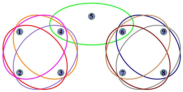
Figure 1: A toy example of a $3$-uniform hypergraph.

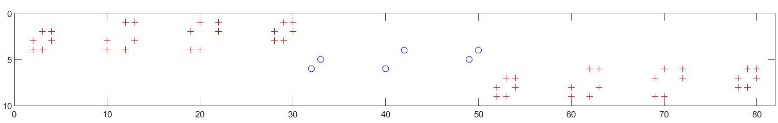
Figure 2: The mode-1 unfolding $\mathbf{R}(\bar{\mathcal{P}})\in\mathbb{R}^{9\times 81}$ of the columnwise-substochastic tensor $\bar{\mathcal{P}}$ is illustrated, where a blue circle and a red plus stand for $1$ and $1/2$ respectively.

Next, to perturb a stochastic vector $\mathbf{u}\in\mathbb{R}^{n}$ ($\mathbf{u}\geq\mathbf{0}$ and $\mathbf{e}^{T}\mathbf{u}=1$) in a quantity $\sigma\in(0,1)$, we utilize an optimization approach for producing a random perturbation $\delta\mathbf{u}\in\mathbb{R}^{n}$ such that $\|\delta\mathbf{u}\|_{1}=\sigma$, $\mathbf{u}+\delta\mathbf{u}\geq\mathbf{0}$, and $\mathbf{e}^{T}(\mathbf{u}+\delta\mathbf{u})=1$. First of all, a random vector $\mathbf{b}\in\mathbb{R}^{n}$ is generated by using the standard normal distribution $N(0,1)$. Then vector $\delta\mathbf{u}$ takes the value from the projection of this random vector $\mathbf{b}$ onto a compact set:

$$\min_{\delta\mathbf{u}\in\mathbb{R}^{n}}~{}\|\delta\mathbf{u}-\mathbf{b}\|_{2}^{2}\quad\mathrm{s.t.}~{}~{}\|\delta\mathbf{u}\|_{1}=\sigma,~{}~{}\mathbf{e}^{T}\delta\mathbf{u}=0,~{}~{}\delta\mathbf{u}\geq-\mathbf{u}.$$

By introducing variables $\mathbf{s}_{+}=\max(\delta\mathbf{u},\mathbf{0})\in\mathbb{R}^{n}_{+}$ and $\mathbf{s}_{-}=\mathbf{s}_{+}-\delta\mathbf{u}\in\mathbb{R}^{n}_{+}$, the above projection problem could be represented as a convex quadratic programming

$$\min{} \|\mathbf{s}_{+}-\mathbf{s}_{-}-\mathbf{b}\|_{2}^{2}$$

$$\mathrm{s.t.}{}{} \mathbf{e}^{T}\mathbf{s}_{+}+\mathbf{e}^{T}\mathbf{s}_{-}=\sigma,~{}~{}\mathbf{e}^{T}\mathbf{s}_{+}-\mathbf{e}^{T}\mathbf{s}_{-}=0,$$

$$\mathbf{s}_{+}-\mathbf{s}_{-}\geq-\mathbf{u},~{}~{}\mathbf{s}_{+}\geq\mathbf{0},~{}~{}\mathbf{s}_{-}\geq\mathbf{0},$$

which could be solved efficiently. Once the optimal solution $(\mathbf{s}_{+},\mathbf{s}_{-})$ of this convex quadratic programming is available, it is straightforward to calculate $\delta\mathbf{u}=\mathbf{s}_{+}-\mathbf{s}_{-}$.

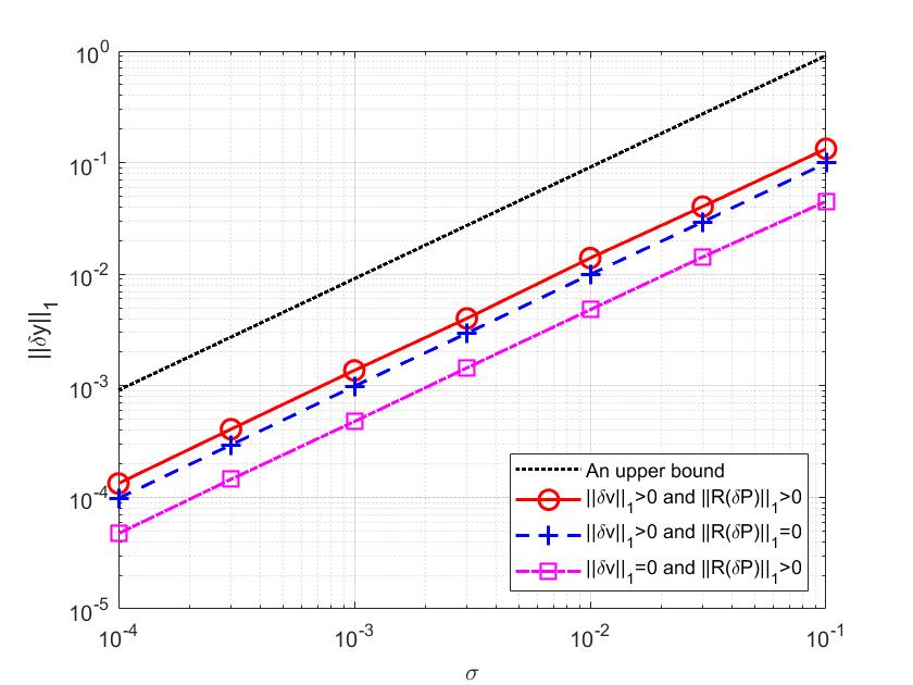
Figure 3: MLPPR solutions vary with various perturbations in the columnwise-substochastic tensor $\bar{\mathcal{P}}$ and a stochastic vector $\mathbf{v}$.

Owing to the difference in coefficients of $\|\delta\mathbf{v}\|_{1}$ and $\|\mathbf{R}(\delta\bar{\mathcal{P}})\|_{1}$ in Theorem 3.13, we set $\|\delta\mathbf{v}\|_{1}=\sigma$ and $\|\mathbf{R}(\delta\bar{\mathcal{P}})\|_{1}=4\sigma$ to balance impacts from $\mathbf{v}$ and $\bar{\mathcal{P}}$, where $\sigma$ is a perturbation quantity. For the columnwise-substochastic tensor $\bar{\mathcal{P}}$, only non-dangling fibers are perturbed. When the perturbation quantity $\sigma$ varies from $0.0001$ to $0.1$, we perform one hundred tests for each $\sigma$ and evaluate the mean of resulting changes $\|\delta\mathbf{y}\|_{1}$ in the MLPPR solution. For comparison, we examine three cases of perturbations: (i) perturb both $\delta\mathbf{v}$ and $\delta\bar{\mathcal{P}}$, (ii) only perturb $\delta\mathbf{v}$, and (iii) only perturb $\delta\bar{\mathcal{P}}$. Numerical results on $\|\delta\mathbf{y}\|_{1}$ versus $\sigma$ are illustrated in Figure 3. The theoretical bound in Theorem 3.13 is also printed here. It is easy to see from Figure 3 that the theoretical bound for $\|\delta\mathbf{y}\|_{1}$ are almost tight up to some constant multiples. In addition, perturbation $\delta\bar{\mathcal{P}}$ has less impact on the MLPPR solution $\mathbf{y}$ than perturbation $\delta\mathbf{v}$.

5.2 Subspace clustering

Subspace clustering BP'13 ; CQZ'17 is a crucial problem in artificial intelligence. A typical problem is to extract subsets of collinear points from a set of points in $\mathbb{R}^{d}$, where $d\geq 2$. In this setting, classical pairwise approaches cannot work. Higher-order similarity of collinear points as well as tensor representions should be exploited.

At the beginning, to identify collinear points, there exists an approach GeoT'99 for computing a least-squares error of fitting a straight line with distinct points $\mathbf{u}_{1},\mathbf{u}_{2},\dots,\mathbf{u}_{k}\in\mathbb{R}^{d}$, where $k\geq 3$. Assume that the straight line goes through $\mathbf{u}_{0}$ with a unit direction $\mathbf{v}$. The cost of least-squares fitting is

$$\Psi(\mathbf{u}_{0},\mathbf{v}):=\sum_{i=1}^{k}\left\|(I-\mathbf{v}\mathbf{v}^{T})(\mathbf{u}_{i}-\mathbf{u}_{0})\right\|^{2}=\sum_{i=1}^{k}(\mathbf{u}_{i}-\mathbf{u}_{0})^{T}(I-\mathbf{v}\mathbf{v}^{T})(\mathbf{u}_{i}-\mathbf{u}_{0}).$$

To find an optimal $\mathbf{u}_{0}$, we consider the partial derivative of the cost $\Psi$ with respect to $\mathbf{u}_{0}$:

$$\frac{\partial\Psi(\mathbf{u}_{0},\mathbf{v})}{\partial\mathbf{u}_{0}}=-2(I-\mathbf{v}\mathbf{v}^{T})\sum_{i=1}^{k}(\mathbf{u}_{i}-\mathbf{u}_{0})=0,$$

of which solutions satisfy $\sum_{i=1}^{k}(\mathbf{u}_{i}-\mathbf{u}_{0})=\varrho\mathbf{v}$ for $\varrho\in\mathbb{R}$. For simplicity, we set $\varrho=0$ and get $\widehat{\mathbf{u}}_{0}=\frac{1}{k}\sum_{i=1}^{k}\mathbf{u}_{i}$. Furthermore, let $U:=[\mathbf{u}_{1}-\widehat{\mathbf{u}}_{0},\dots,\mathbf{u}_{k}-\widehat{\mathbf{u}}_{0}]\in\mathbb{R}^{d\times k}$. The cost $\Psi$ could be rewritten as

$$\Psi(\widehat{\mathbf{u}}_{0},\mathbf{v})=\mathrm{trace}(U^{T}U)-\mathbf{v}^{T}UU^{T}\mathbf{v}.$$

To minimize the cost $\Psi$, an optimal (unit) direction $\widehat{\mathbf{v}}$ has a closed-form solution: the eigenvector corresponding to the largest eigenvalue of $UU^{T}$.

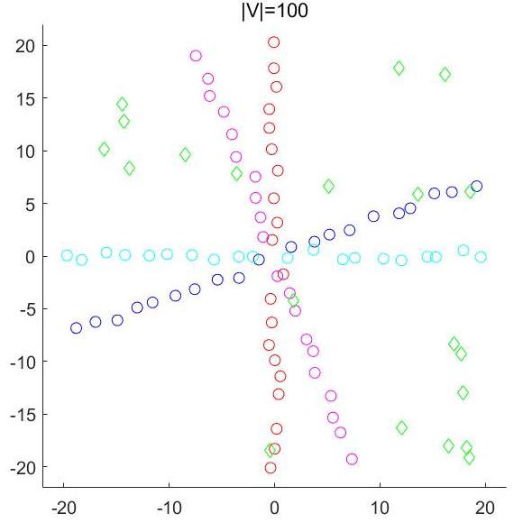
(a)	(b)

Figure 4: Illustrations of points for subspace clustering. Points of various colors (blue, cyan, magenta, and red) are located in different subspaces. Green diamonds are outliers.

Next, we consider clustering multiple subspaces. Fig. 4(a) illustrates one hundred points, which constitute roughly four subsets of collinear points with blue, cyan, magenta, and red colors located in lines (subspaces) with slopes $\pi/9$, $0$, $-7\pi/18$, and $-\pi/2$, respectively. All points are corrupted by additive Gaussian noise $N(0,1/2)$. Each subset has twenty percent of points and the remainder are outliers that are marked as green diamonds. A larger example with two thousand points is displayed in Fig. 4(b). When only positions of these points are known, how can we cluster these points such that points in each subset are nearly collinear?

As a first step, we construct an undirected $3$-uniform hypergraph $G=(V,E,\mathbf{w})$. Each point is regarded as a vertex in $V$. Hence, $\lvert V\rvert=n$. Basically, every three vertices may be connected as an edge to produce a complete $3$-uniform hypergraph. But it is too expensive to handle complete hypergraphs in practice. We prefer to use a random hypergraph which is generated by two steps economically. (i) To ensure connectedness, a complete graph is produced in advance. Then, for each edge of the complete graph, we add a different vertex which is randomly chosen. So there are $n(n-1)/2$ edges as candidates. (ii) For every candidate edge, we compute the least-squares error of fitting a straight line with positions of three points in a candidate edge. Then five percent candidate edges with smaller fitting errors are picked up to form $m:=\lvert E\rvert=[n(n-1)/40]$ edges of a random $3$-uniform hypergraph. All weights of edges of this hypergraph are ones.

Algorithm 2 MLPPR-based hypergraph bipartition.

1:Form a $3$-uniform hypergraph $G$, generate its adjacency tensor $\mathcal{A}$ by (4) and then a columnwise-substochastic tensor $\bar{\mathcal{P}}$ by (6).

2:Choose a probability $\alpha=0.99$ and a stochastic vector $\mathbf{v}=\mathbf{e}/n$.

3:Solve MLPPR (7) by Algorithm 1 for a nonnegative solution $\mathbf{y}_{*}$.

4:Form $\widehat{A}=\bar{\mathcal{P}}\times_{3}\mathbf{y}_{*}$ as an adjacency matrix of a latent directed graph.

5:Compute $D=\mathrm{diag}(\mathbf{e}^{T}\widehat{A})$ and $\bar{P}=\widehat{A}D^{-1}$. Find $\mathbf{\pi}$ such that $\bar{P}\mathbf{\pi}=\mathbf{\pi}$.

6:Let $\Pi=\mathrm{diag}(\mathbf{\pi})$. Find the second left eigenvector $\mathbf{x}_{*}$ of $2P_{\mathrm{sym}}=\Pi\bar{P}^{T}\Pi^{-1}+\bar{P}$.

7:Use $\mathbf{x}_{*}$ to produce a bipartition of the vertex set of the given hypergraph $G$.

Once a random hypergraph is ready, our approach, i.e., Algorithm 2 using MLPPR, follows the framework of Algorithm 1 in BGL'15 . Roughly speaking, there are two stages. (i) MLPPR-based Hypergraph analysis. Above all, we generate an adjacency tensor $\mathcal{A}$ and a columnwise-substochastic tensor $\bar{\mathcal{P}}$ of a random $3$-uniform hypergraph. By setting a probability $\alpha=0.99$ and a stochastic vector $\mathbf{v}=\mathbf{e}/n$, an MLPPR problem is solved by the tensor splitting algorithm to obtain a nonnegative solution $\mathbf{y}_{*}$. (ii) Unsupervised clustering of a directed graph BGL'15 ; Ch'05 . Let $\widehat{A}:=\bar{\mathcal{P}}\times_{3}\mathbf{y}_{*}\in\mathbb{R}^{n\times n}$ be an adjacency matrix of a latent directed graph. It is straightforward to calculate a degree matrix $D=\mathrm{diag}(\mathbf{e}^{T}\widehat{A})$ and a columnwise-stochastic matrix $\bar{P}=\widehat{A}D^{-1}$. By a symmetrized approach in Ch'05 , we set $\Pi:=\mathrm{diag}(\mathbf{\pi})$, where $\mathbf{\pi}\in\mathbb{R}^{n}_{+}$ is the stationary distribution of $\bar{P}$ such that $\bar{P}\mathbf{\pi}=\mathbf{\pi}$. Then, we define $A_{\mathrm{sym}}:=\frac{1}{2}(\Pi\bar{P}^{T}+\bar{P}\Pi)$, $D_{\mathrm{sym}}=\mathrm{diag}(A_{\mathrm{sym}}\mathbf{e})=\Pi$, and $P_{\mathrm{sym}}=A_{\mathrm{sym}}D_{\mathrm{sym}}^{-1}=\frac{1}{2}(\Pi\bar{P}^{T}\Pi^{-1}+\bar{P})$. Finally, the second left eigenvector of $P_{\mathrm{sym}}$ is calculated for partitioning vertices of this hypergraph.

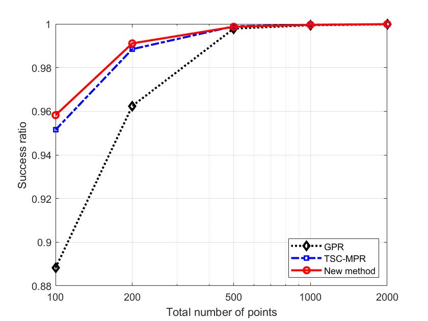
Figure 5: Success ratio of various methods

To produce a bipartition of the vertex set $V$ of a $3$-uniform hypergraph $G$, i.e., Step 7 of Algorithm 2, we utilize the normalized cut of hypergraphs. For a vertex subset $\emptyset\subset S\subset V$, we define the volume of $S$:

$$\mathrm{vol}(S):=\sum_{i,j,k\atop i\in S}a_{ijk},$$

where $a_{ijk}$’s are elements of an adjacency tensor of $G$. Let $\bar{S}:=V\backslash S$. The cut of $S$ is defined as

$$\mathrm{cut}(S):=\sum_{i,j,k}a_{ijk}-\sum_{i,j,k\in S}a_{ijk}-\sum_{i,j,k\in\bar{S}}a_{ijk}.$$

Then, the normalized cut of $G$ is defined as follows

$$h=\min_{\emptyset\subset S\subset V}\mathrm{cut}(S)\left(\frac{1}{\mathrm{vol}(S)}+\frac{1}{\mathrm{vol}(\bar{S})}\right).$$

Indeed, it is NP-hard to evaluate normalized cuts of hypergraphs exactly. A heuristic and economic approach is widely used. We sort vertices in $V$ of $G$ according to the corresponding elements of the second left eigenvector $\mathbf{x}_{*}$ of $P_{\mathrm{sym}}$ to obtain an ordered arrangement $\nu_{1},\nu_{2},\dots,\nu_{n}$ of vertices in $V$. To find an efficient cut, we only consider subsets $S$ that contains the leading vertices of this ordered arrangement. That is to say, we compute

$$h(i)=\mathrm{cut}(\{\nu_{1},\dots,\nu_{i}\})\left(\frac{1}{\mathrm{vol}(\{\nu_{1},\dots,\nu_{i}\})}+\frac{1}{\mathrm{vol}(\{\nu_{i+1},\dots,\nu_{n}\})}\right)$$ (21)

for $i=1,\dots,n-1$ and then pick up the optimal index $i_{*}$ such that

$$i_{*}=\mathop{\arg\min}_{1\leq i\leq n-1}h(i).$$ (22)

The minimization (22) is a heuristic approximation of the normalized cut of $G$. Then, a solution $i_{*}$ of (22) produces a bipartition of points corresponding to vertex subsets $\{\nu_{1},\dots,\nu_{i_{*}}\}$ and $\{\nu_{i_{*}+1},\dots,\nu_{n}\}$ of $G$. Whereafter, since there are four subspaces in our experiments, we recursively run Algorithm 2 to repartition a sub-hypergraph with a larger vertex subset of $G$ until the set of points are clustered in four parts.

A significant difference between our method and Algorithm 1 in BGL'15 (named TSC-MPR) is that the former do not use any dangling information but the latter do. On one hand, for large-scale (sparse) random hypergraphs, there are a mount of dangling fibers contained in adjacency tensors of hypergraphs. By discarding dangling information, MLPPR is more efficient than MPR. On the other hand, although the stochastic vector $\mathbf{y}_{*}/(\mathbf{e}^{T}\mathbf{y}_{*})$, where $\mathbf{y}_{*}$ is generated by MLPPR, is the same as the solution $\mathbf{x}_{*}$ of MPR, the matrix $\widehat{A}=\bar{\mathcal{P}}\times_{3}\mathbf{y}_{*}$ in Step 4 of Algorithm 2 is different from $\mathcal{P}\times_{3}\mathbf{x}_{*}$ used in TSC-MPR. Since the tensor $\mathcal{P}$ is a columnwise-stochastic tensor with dangling corrections, the matrix $\mathcal{P}\times_{3}\mathbf{x}_{*}$ is also columnwise-stochastic. When we give up dangling corrections, the matrix $\widehat{A}=\bar{\mathcal{P}}\times_{3}\mathbf{y}_{*}$ is only nonnegative but not necessarily columnwise-stochastic. In this sense, the matrix $\widehat{A}=\bar{\mathcal{P}}\times_{3}\mathbf{y}_{*}$ is clean while the matrix $\mathcal{P}\times_{3}\mathbf{x}_{*}$ may be corrupted by dangling corrections.

For solving subspace clustering problems, we run three methods: (i) The new method, i.e., Algorithm 2 using MLPPR. (ii) TSC-MPR: tensor spectral clustering by MPR in BGL'15 . (iii) GPR: PageRank for a graph approximation of a hypergraph. For subspace clustering problems with total numbers of points ranging from $100$ to $2000$, we count the success ratios of points being in correct clusters, where outliers could be in any clusters. For each case, we run 100 tests with randomly generated points. Numerical results illustrated in Fig. 5 means that the new method outperforms TSC-MPR and GPR. Owing to the skilful avoiding of dangling corrections, the new method is effective and efficient.

5.3 Network analysis

Higher-order graph information is important for analyzing network. For example, triangles (network structures involving three nodes) are fundamental to understand social network and community structure KW06 ; RELWL14 ; BGL16 ; BGL'17 . Particularly, we are interested in the directed 3-cycle (D3C), which captures a feedback loop in network.

Table 1: Information of networks and partition sizes.

Network	#nodes	#D3Cs	GPR	TSC-MPR	New method
email-EuAll	11,315	183,836	1,492	1,700	1,634
wiki-Talk	52,411	5,138,613	21,893	21,240	21,238

We consider two practical networks snapnets in Table 1 from https://snap.stanford.edu/data/. Originally, each network is a directed graph. For instance, each node in the “email-EuAll” network represents an email address. There exists a directed edge from nodes $i$ to $j$ if $i$ sent at least one message to $j$. Before higher-order network analysis, we filter the network as follows: (i) remove all vertices and all edges that do not participate in any D3Cs; (ii) take the largest strongly connected component of the remaining network. As a result, the filtered “email-EuAll” network contains $11,315$ nodes and $183,836$ D3Cs. A larger network named “wiki-Talk” contains $52,411$ nodes and $5,138,613$ D3Cs.

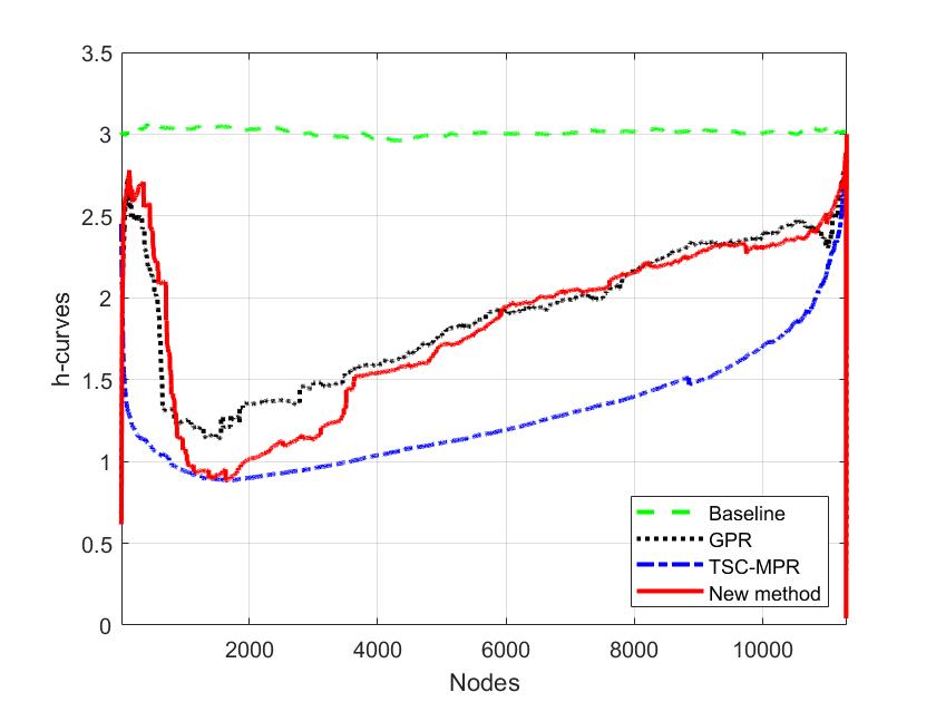
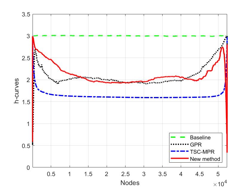
(a) “email-EuAll” network	(b) “wiki-Talk” network

Figure 6: $h$-curves of networks.

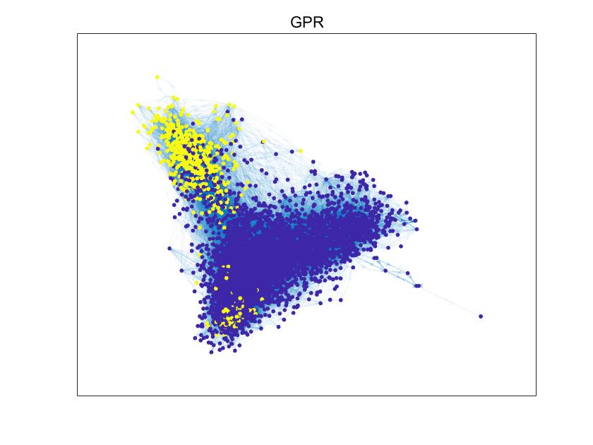
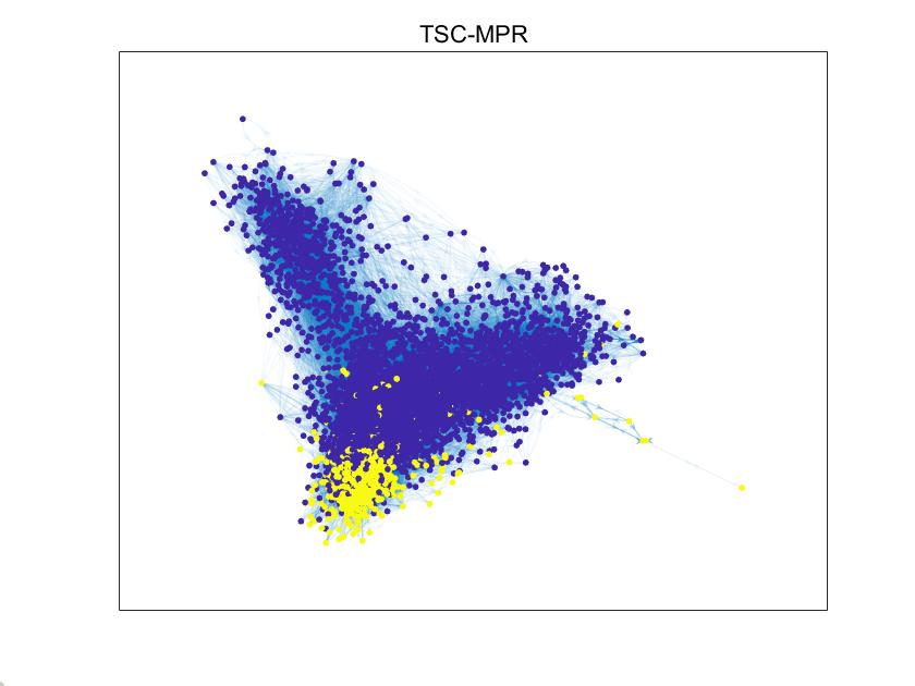
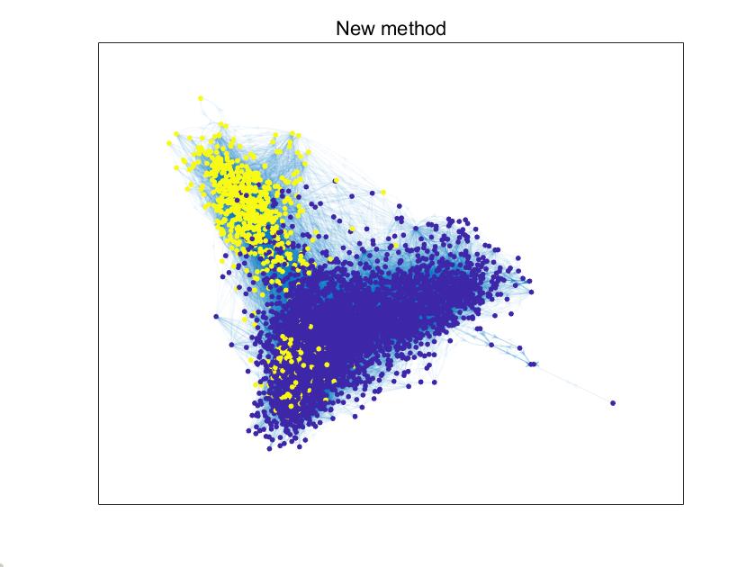
(a)	(b)	(c)
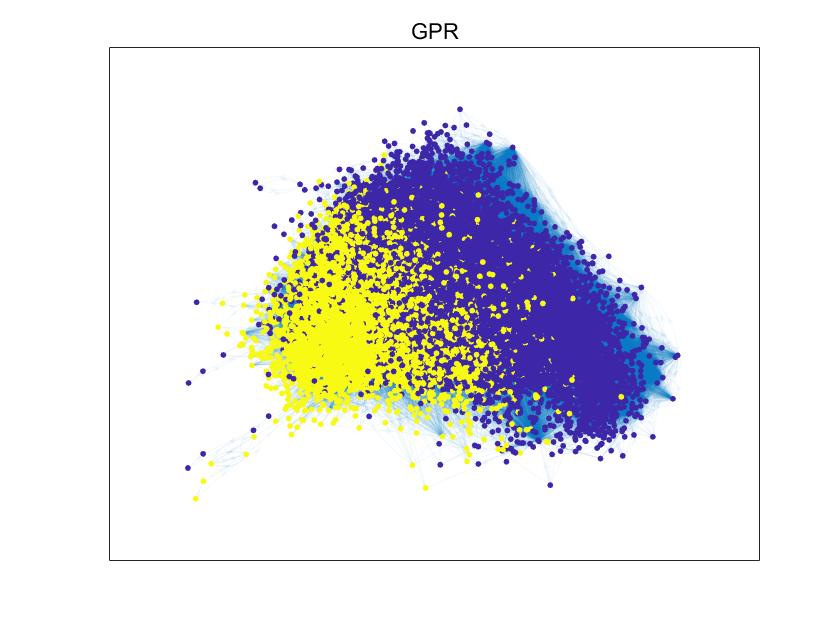
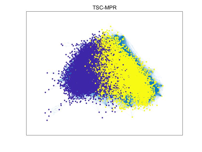
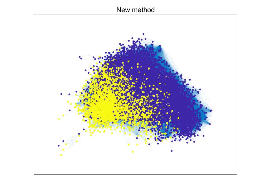
(d)	(e)	(f)

Figure 7: Illustration of partitioned results. Results of the “email-EuAll” network are displayed in (a–c) and results of the “wiki-Talk” network are displayed in (d–f).

Then it is straightforward to construct a $3$-uniform hypergraph $G$, where nodes and D3Cs of a network are vertices and edges of a $3$-uniform hypergaph, respectively. All weights are set to ones. To produce heuristic and efficient cuts, we test four algorithms for generating ordered arrangements of vertices of a hypergraph: (i) Baseline: a random order, (ii) GPR: PageRank for a graph approximation of a hypergraph, (iii) TSC-MPR: tensor spectral clustering by MPR in BGL'15 , and (iv) the new method, i.e., Algorithm 2 using MLPPR. By experiments, four algorithms generate four orders, of which associated $h$-curves defined by (21) are illustrated in Fig. 6. By picking up a minimum of $h$ by (22), each algorithm obtains a partition. The new method returns bipartitions with $\lvert S\rvert=1,634$ nodes for the “email-EuAll” network and $\lvert S\rvert=21,238$ nodes for the “wiki-Talk” network, as illustrated respectively in Fig. 7 (c) and (f). Partitions produced by TSC-MPR and GPR are also reported in Fig. 7 and associated partition sizes are listed in Table 1. When compared with these existing methods, the new method is competitive.

Table 2: CPU times (seconds).

Network	MPR-1	MPR-2	MLPPR
email-EuAll	1.882	0.073	0.064
wiki-Talk	58.530	2.257	0.913

Finally, we examine CPU times costed by solving MPR and MLPPR problems. MLPPR problems are solved by the tensor splitting algorithm and MPR problems are solved by the shifted fixed-point iteration BGL'15 ; GLY'15 . We should remind readers that CPU times costed by any existing algorithms for solving MPR and MLPPR are just a little part of the time for handling the whole process of network analysis. We recall the dangling correction (14) used by MPR:

$$\mathcal{P}:=\bar{\mathcal{P}}+\mathbf{v}\circ\underbrace{\left(\mathbf{e}^{\circ(k-1)}-\bar{\mathcal{P}}\bar{\times}_{1}\mathbf{e}\right)}_{:=\mathcal{C}}\in\mathbb{R}^{[k,n]}_{+},$$

where $\mathcal{C}$ is a $(k-1)$th order indicator tensor of dangling fibers of $\bar{\mathcal{P}}$. On one hand, a straightforward approach (MPR-1) is to save and to manipulate $\mathcal{C}$ explicitly. On the other hand, if $\mathcal{C}$ is dense but $\mathbf{e}^{\circ(k-1)}-\mathcal{C}$ is sparse, an alternative approach (MPR-2) utilizes $\mathbf{e}^{\circ(k-1)}-\mathcal{C}$ explicitly. For solving MPR/MLPPR problems raising from “email-EuAll” and “wiki-Talk” networks, CPU times (in seconds) of MPR-1, MPR-2, and MLPPR are reported in Table 2. Obviously, MPR-2 is faster than MPR-1. This verifies that indicator tensors $\mathcal{C}$ are dense. Particularly, MLPPR is about 60 times faster than MPR-1 when dealing with “wiki-Talk” network. According to these numerical experiments, the proposed MLPPR is powerful and efficient.

6 Conclusions

As an interesting extension of the classical PageRank model for graph partitioning, we proposed the MLPPR model for partitioning uniform hypergraphs. By using Laplacian tensors of uniform hypergraphs without any dangling corrections, MLPPR is more suitable for processing large-scale hypergraphs. The existence and uniqueness of nonnegative solutions of MLPPR were analyzed. An error bound of the MLPPR solution was analyzed when the Laplacian tensor and a stochastic vector are slightly perturbed. By exploiting the structural Laplacian tensors, we designed a tensor splitting algorithm (a fixed-point iterations) for MLPPR. Numerical experiments on subspace clustering and network analysis verified the powerfulness and effectiveness of our method.

Funding This work was funded by the National Natural Science Foundation of China grant 12171168, 12071159, 11901118, 11771405, 62073087 and U1811464.

Data Availability The data that support the findings of this study are available from the corresponding author upon reasonable request.

Declarations

Conflict of interest The authors have no relevant financial or non-financial interests to disclose.

References

• \bibcommenthead
• (1) Brin, S., Page, L.: The anatomy of a large-scale hypertextual Web search engine. Computer Networks and ISDN Systems 30(1), 107–117 (1998). https://doi.org/10.1016/S0169-7552(98)00110-X
• (2) Bryan, K., Leise, T.: The $\$25,000,000,000$ eigenvector: The linear algebra behind Google. SIAM Review 48(3), 569–581 (2006). https://doi.org/10.1137/050623280
• (3) Gleich, D.F.: PageRank beyond the Web. SIAM Review 57(3), 321–363 (2015). https://doi.org/10.1137/140976649
• (4) Langville, A.N., Meyer, C.D.: Google’s PageRank and Beyond: The Science of Search Engine Rankings. Princeton university press, Princeton (2006)
• (5) Benson, A.R., Gleich, D.F., Leskovec, J.: Higher-order organization of complex networks. Science 353(6295), 163–166 (2016). https://doi.org/10.1126/science.aad9029
• (6) Benson, A.R., Gleich, D.F., Lim, L.-H.: The spacey random walk: A stochastic process for higher-order data. SIAM Review 59(2), 321–345 (2017). https://doi.org/10.1137/16M1074023
• (7) Kossinets, G., Watts, D.J.: Empirical analysis of an evolving social network. Science 311(5757), 88–90 (2006). https://doi.org/10.1126/science.1116869
• (8) Rosvall, M., Esquivel, A.V., Lancichinetti, A., West, J.D., Lambiotte, R.: Memory in network flows and its effects on spreading dynamics and community detection. Nature Communications 5, 4630 (2014). https://doi.org/10.1038/ncomms5630
• (9) Ipsen, I.C.F., Selee, T.M.: PageRank computation, with special attention to dangling nodes. SIAM Journal on Matrix Analysis and Applications 29(4), 1281–1296 (2008). https://doi.org/10.1137/060664331
• (10) Francesco, T.: A note on certain ergodicity coefficients. Special Matrices 3(1), 175–185 (2015). https://doi.org/10.1515/spma-2015-0016
• (11) Langville, A.N., Meyer, C.D.: A reordering for the pagerank problem. SIAM Journal on Scientific Computing 27(6), 2112–2120 (2006). https://doi.org/10.1137/040607551
• (12) Chung, F.: Laplacians and the Cheeger inequality for directed graphs. Annals of Combinatorics 9(1), 1–19 (2005). https://doi.org/10.1007/s00026-005-0237-z
• (13) Andersen, R., Chung, F., Lang, K.: Using PageRank to locally partition a graph. Internet Mathematics 4(1), 35–64 (2007)
• (14) Andersen, R., Chung, F., Lang, K.: Local partitioning for directed graphs using PageRank. Internet Mathematics 5(1-2), 3–22 (2008). https://doi.org/im/1259158595
• (15) Li, W., Ng, M.K.: On the limiting probability distribution of a transition probability tensor. Linear and Multilinear Algebra 62(3), 362–385 (2014). https://doi.org/10.1080/03081087.2013.777436
• (16) Gleich, D.F., Lim, L.-H., Yu, Y.: Multilinear PageRank. SIAM Journal on Matrix Analysis and Applications 36(4), 1507–1541 (2015). https://doi.org/10.1137/140985160
• (17) Chang, K.C., Zhang, T.: On the uniqueness and non-uniqueness of the positive Z-eigenvector for transition probability tensors. Journal of Mathematical Analysis and Applications 408(2), 525–540 (2013). https://doi.org/10.1016/j.jmaa.2013.04.019
• (18) Fasino, D., Tudisco, F.: Ergodicity coefficients for higher-order stochastic processes. SIAM Journal on Mathematics of Data Science 2(3), 740–769 (2020). https://doi.org/10.1137/19M1285214
• (19) Li, W., Liu, D., Ng, M.K., Vong, S.-W.: The uniqueness of multilinear PageRank vectors. Numerical Linear Algebra with Applications 24(6), 2107–112 (2017). https://doi.org/10.1002/nla.2107
• (20) Li, W., Liu, D., Vong, S.-W., Xiao, M.: Multilinear PageRank: Uniqueness, error bound and perturbation analysis. Applied Numerical Mathematics 156, 584–607 (2020). https://doi.org/10.1016/j.apnum.2020.05.022
• (21) Li, W., Cui, L.-B., Ng, M.K.: The perturbation bound for the Perron vector of a transition probability tensor. Numerical Linear Algebra with Applications 20(6), 985–1000 (2013). https://doi.org/10.1002/nla.1886
• (22) Benson, A.R.: Three hypergraph eigenvector centralities. SIAM Journal on Mathematics of Data Science 1(2), 293–312 (2019). https://doi.org/10.1137/18M1203031
• (23) Benson, A.R., Gleich, D.F., Leskovec, J.: Tensor Spectral Clustering for Partitioning Higher-order Network Structures. In: Proc SIAM Int Conf Data Min., pp. 118–126 (2015)
• (24) Meini, B., Poloni, F.: Perron-based algorithms for the multilinear PageRank. Numerical Linear Algebra with Applications 25(6), 2177–115 (2018). https://doi.org/10.1002/nla.2177
• (25) Huang, J., Wu, G.: Convergence of the fixed-point iteration for multilinear PageRank. Numerical Linear Algebra with Applications 28(5), 2379 (2021). https://doi.org/10.1002/nla.2379
• (26) Liu, D., Li, W., Vong, S.-W.: Relaxation methods for solving the tensor equation arising from the higher-order Markov chains. Numerical Linear Algebra with Applications 26(5), 2260 (2019). https://doi.org/10.1002/nla.2260
• (27) Cipolla, S., Redivo-Zaglia, M., Tudisco, F.: Extrapolation methods for fixed-point multilinear PageRank computations. Numerical Linear Algebra with Applications 27(2), 2280 (2020). https://doi.org/10.1002/nla.2280
• (28) Yuan, A., Calder, J., Osting, B.: A continuum limit for the PageRank algorithm. European Journal of Applied Mathematics 33(3), 472–504 (2022). https://doi.org/10.1017/S0956792521000097
• (29) Bulò, S.R., Pelillo, M.: A game-theoretic approach to hypergraph clustering. IEEE Transactions on Pattern Analysis and Machine Intelligence 35(6), 1312–1327 (2013). https://doi.org/10.1109/TPAMI.2012.226
• (30) Cooper, J., Dutle, A.: Spectra of uniform hypergraphs. Linear Algebra and its Applications 436(9), 3268–3292 (2012). https://doi.org/10.1016/j.laa.2011.11.018
• (31) Qi, L., Luo, Z.: Tensor Analysis: Spectral Theory and Special Tensors. SIAM, Philadelphia (2017)
• (32) Gao, G., Chang, A., Hou, Y.: Spectral radius on linear $r$-graphs without expanded $k_{r+1}$. SIAM Journal on Discrete Mathematics 36(2), 1000–1011 (2022). https://doi.org/10.1137/21M1404740
• (33) Li, W., Ng, M.K.: Some bounds for the spectral radius of nonnegative tensors. Numerische Mathematik 130, 315–335 (2015). https://doi.org/10.1007/s00211-014-0666-5
• (34) Liu, C.-S., Guo, C.-H., Lin, W.-W.: Newton–Noda iteration for finding the Perron pair of a weakly irreducible nonnegative tensor. Numerische Mathematik 137, 63–90 (2017). https://doi.org/10.1007/s00211-017-0869-7
• (35) Chen, Y., Qi, L., Zhang, X.: The Fiedler vector of a Laplacian tensor for hypergraph partitioning. SIAM Journal on Scientific Computing 39(6), 2508–2537 (2017). https://doi.org/%****␣MLPPR20221201.tex␣Line␣1950␣****10.1137/16M1094828
• (36) Eberly, D.: Least Squares Fitting of Data by Linear or Quadratic Structures, Redmond WA 98052 (Created: July 15, 1999; Last Modified: September 7, 2021)
• (37) Leskovec, J., Krevl, A.: SNAP datasets: Stanford large network dataset collection (2014)