Hyperspectral super-resolution via low rank tensor triple decomposition

Abstract.

Hyperspectral image (HSI) and multispectral image (MSI) fusion aims at producing a super-resolution image (SRI). In this paper, we establish a nonconvex optimization model for image fusion problems through low-rank tensor triple decomposition. Using the L-BFGS approach, we develop a first-order optimization algorithm for obtaining the desired super-resolution image (TTDSR). Furthermore, two detailed methods are provided for calculating the gradient of the objective function. With the aid of the Kurdyka-$\L$ ojasiewicz property, the iterative sequence is proved to converge to a stationary point. Finally, experimental results on different datasets show the effectiveness of our proposed approach.

Xiaofei Cui${}^{{\href mailto:cuixiaofei3583@163.com}1}$ and Jingya Chang${}^{{\href mailto:jychang@gdut.edu.cn.com}*1}$

¹School of Mathematics and Statistics, Guangdong University of Technology, China

(Communicated by Jingya Chang)

1. Introduction

Equipment for hyperspectral imaging uses an unusual sensor to produce images with great spectral resolution. The key factor in an image is the electromagnetic spectrum obtained by sampling at hundreds of continuous wavelength intervals. Because hyperspectral images have hundreds of bands, spectral information is abundant [32]. Hyperspectral images are now the core of a large and increasing number of remote sensing applications, such as environmental monitoring [4, 25], target classification [41, 8] and anomaly detection [7, 37].

With optical sensors, there is a fundamental compromise among spectral resolution, spatial resolution and signal-to-noise ratio. Hyperspectral images therefore have a high spectral resolution but a low spatial resolution. Contrarily, multispectral sensors, which only have a few spectral bands, can produce images with higher spatial resolution but poorer spectral resolution [5].

The approaches for addressing hyperspectral and multispectral images fusion issues can be categorized into four classes [42]. The generalized sharpening approach falls within the first category. A pan-sharpening strategy for extending to hyperspectral and multispectral images fusion was presented, such as component substitution [27, 1] and multiresolution analysis [16]. Selva et al. [30] applied multi-resolution analysis method to extract spatial details and injected it into the interpolated hyperspectral image. Liu et al. [22] injected high frequency spatial details from multispectral image into hyperspectral image using the same strategy. Chen et al. [9] divided all bands of the images into several regions and then fused the images of each region by universal sharpening algorithm. Unfortunately, these pan-sharpening methods may lead to spectral distortion. The second category is subspace-based formulas. The main idea is to explore the natural low-dimensional representation of hyperspectral image, and regard it as a linear combination of a set of basis vectors or spectral features [18, 38, 34]. Hardie et al. [15] employed Bayesian formulas to solve the super-resolution image issues by the maximum posteriori probability. The method based on matrix factorization falls within the third category. Under these circumstances, HSI and MSI are regarded as the degradation versions of SRI. Yokoya et al. [40] proposed a coupled nonnegative matrix factorization method, which estimates the basic vectors and its coefficients blindly and then calculates the endmember and degree matrix by alternating optimization algorithm. In addition, there are matrix factorizations using sparse regularization and spatial regularization [19, 31], such as a low rank matrix decomposition model for decomposing hyperspectral image into a super-resolution image and a difference image in [12, 42].

Tensor decomposition methods fall within the fourth category. Tensor, a higher-order extension of matrix, can capture the correlation between the spatial and spectral domains in hyperspectral images simultaneously. Representing hyperspectral and multispectral images as third-order tensors has been widely used in hyperspectral image denoising and super-resolution problems. The hyperspectral image is a three-dimensional data cube with two spatial dimensions (height and width) and one spectral dimension [17, 33, 23]. The spatial details and spectral structures of the target SRI therefore are both more accurate.

The superior resolution performance and exact recovery guarantee are attained for the low rank of hyperspectral images by low rank tensor decomposition techniques. Kanatsoulis et al. [20] proposed treating the image fusion problem as a coupled tensor approximation, where they assumed the super-resolution image satisfies a low rank Canonical Polynomial (CP) decomposition. Later, Li et al. [28, 24] considered a novel approach based on tensor Tucker decomposition. Xu et al. [39] first considered that the target SRI exhibits both the sparsity and the piecewise smoothness on the three modes and then utilize the classical tensor Tucker decomposition to decompose the target SRI. Dian et al. [13] applied tensor kernel norm to explore low rank property of SRI. He et al. [16] proposed a tensor ring decomposition method for addressing the image fusion.

In this paper, we propose a novel model based on low rank triple decomposition to address the hyperspectral and multispectral images fusion problem. Triple decomposition breaks down a third-order tensor into three smaller tensors with predetermined dimensions. It is frequently applied in tensor completion and image restoration [29, 11]. The image fusion and tensor triple decomposition structures are presented in Fig.1. The optimization model is solved by the limited memory BFGS (L-BFGS) algorithm. Also, the convergent results are given with the help of Kurdyka-$\L$ojasiewicz property of the objective function. Numerical experiments demonstrate that the proposed TTDSR method performs well and the convergent conclusion is also validated numerically.

The rest of this paper is organized as follows. In Sect.2, we first provide definitions used in the paper and present the basic algebraic operations of tensors. In Sect.3, we introduce our model for the hyperspectral and multispectral images fusion. In Sect.4, the L-BFGS algorithm and the gradient calculation are also presented in detail. Convergence analysis of the algorithm is available in Sect.5. In Sect.6, experimental results on two data sets are given. The conclusion is given in Sect.7.

2. Preliminary

Let $\mathbb{R}$ be the real field. We use lowercase letters and boldface lowercase letters to represent scalars and vectors respectively, while capital letters and calligraphic letters stand for matrices and tensors respectively.

An $m$th order $n$ dimensional tensor $\mathcal{A}$ is a multidimensional array with its entry being

$$\mathcal{A}_{i_{1},i_{2},\ldots,i_{m}}=a_{i_{1},i_{2},\ldots,i_{m}},\ \text{for}\ i_{j}=1,\ldots,n,j=1,\ldots,m.$$

Similarly, the $i$th entry in a vector a is symbolized by $(\mathbf{a})_{i}=a_{i}$, and the $(i,j)$th entry of a matrix $A$ is $(A)_{ij}=a_{ij}.$ Unless otherwise specified, the order of tensor is set to three hereafter in this paper. Without loss of generality, we denote $\mathcal{A}\in\mathbb{R}^{n_{1}\times n_{2}\times n_{3}}.$ A fiber of $\mathcal{A}$ is a vector produced by fixing two indices of $\mathcal{A},$ such as $\mathcal{A}(i,j,:)$ for any $i\in[1,\ldots,n_{1}],j\in[1,\ldots,n_{2}]$. A slice of $\mathcal{A}$ is a matrix by varying two of its indices while fixing another one, such as $\mathcal{A}(:,:,k)$ for any $k\in[1,\ldots,n_{3}].$ The geometric structures of the tensor expansion are shown in Fig.2.

The mode-$k$ product of the tensor $\mathcal{A}$ and a matrix $X$ is an extension of matrix product. Suppose matrices $F\in\mathbb{R}^{l\times n_{1}}$, $G\in\mathbb{R}^{m\times n_{2}}$, and $H\in\mathbb{R}^{n\times n_{3}}$. The mode-$1$ product of $\mathcal{A}$ and $F$ is denoted as $\mathcal{A}\times_{1}F$ with its elements being

$$\left(\mathcal{A}\times_{1}{F}\right)_{tjk}=\sum_{i=1}^{n_{1}}a_{ijk}f_{ti},\quad\text{for}\ t=1,\ldots l,j=1,\ldots,n_{2},k=1,\ldots n_{3}.$$

Also we have

$$\left(\mathcal{A}\times_{2}{G}\right)_{ipk}=\sum_{j=1}^{n_{2}}a_{ijk}g_{pj},\quad\left(\mathcal{A}\times_{3}{H}\right)_{ijq}=\sum_{k=1}^{n_{3}}a_{ijk}h_{qk},\quad$$ (1)

for $p=1,\ldots m,$ $q=1,\ldots,n.$ It is easy to verify that

$$\begin{split}\mathcal{A}\times_{p}{F}\times_{q}{G}=&\mathcal{A}\times_{q}{G}\times_{p}{F},\quad\forall\ p,q=1,2,3\ \text{and}\ p\neq q,\\ \mathcal{A}\times_{k}{F}\times_{k}{G}=&\mathcal{A}\times_{k}({GF}),\quad\forall\ k=1,2,3.\end{split}$$ (2)

The mode-$k$ matricization of $\mathcal{A}$ denoted by ${A}_{(k)}$ arranges its $n_{k}$ mode-$k$ fibers as the columns of $A_{(k)}$ in order. The Frobenius norm of tensor $\mathcal{A}$ is given by

$$\|\mathcal{A}\|_{F}=\left(\sum_{i=1}^{n_{1}}\sum_{j=1}^{n_{2}}\sum_{k=1}^{n_{3}}a_{ijk}^{2}\right)^{1/2}.$$ (3)

The unfolding related no matter with tensors, matrices or vectors in the following part is carried out under the precondition that the left index varies more rapidly than the right one. Subscript represents dimension. We note that ${vec}\left(B_{m\times n}\right)$ creates a column vector $\mathbf{b}_{mn}$ by stacking the columns of $B_{m\times n}$ below one another, i.e., $\left(\mathbf{b}_{mn}\right)_{i+(j-1)m}=b_{ij}$. In addition, the kronecker product of matrices $B_{m\times n}$ and $C_{p\times q}$ is

$$B_{m\times n}\otimes C_{p\times q}=\left(\begin{array}[]{cccc}b_{11}C_{p\times q}&b_{12}C_{p\times q}&\cdots&b_{1n}C_{p\times q}\\ b_{21}C_{p\times q}&b_{22}C_{p\times q}&\cdots&b_{2n}C_{p\times q}\\ \cdots&\cdots&\cdots&\cdots\\ b_{m1}C_{p\times q}&b_{m2}C_{p\times q}&\cdots&b_{mn}C_{p\times q}\end{array}\right),\quad$$

for $s=1,\cdots,p,$ $t=1,\cdots,q.$ It generates a large matrix $D_{pm\times qn}=B_{m\times n}\otimes C_{p\times q}$, whose entries are ${d}_{gh}=b_{ij}c_{st}$ with $g=s+(i-1)p$ and $h=t+(j-1)q$. By this rule, unfolding matrices of tensor $\mathcal{A}$ could be represented by

$$\begin{split}\left(A_{n_{1}\times n_{2}n_{3}}\right)_{i,j+(k-1)n_{2}}=a_{ijk},\quad&\left(A_{n_{1}\times n_{3}n_{2}}\right)_{i,k+(j-1)n_{3}}=a_{ijk},\\ \left(A_{n_{2}\times n_{3}n_{1}}\right)_{j,k+(i-1)n_{3}}=a_{ijk},\quad&\left(A_{n_{2}\times n_{1}n_{3}}\right)_{j,i+(k-1)n_{1}}=a_{ijk},\\ \left(A_{n_{3}\times n_{1}n_{2}}\right)_{k,i+(j-1)n_{1}}=a_{ijk},\quad&\left(A_{n_{3}\times n_{2}n_{1}}\right)_{k,j+(i-1)n_{2}}=a_{ijk}.\end{split}$$ (4)

Moreover, $A_{n_{1}n_{2}\times n_{3}}=\left(A_{n_{3}\times n_{1}n_{2}}\right)^{\top}.$

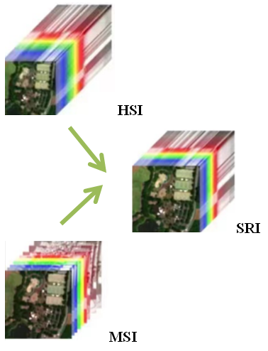
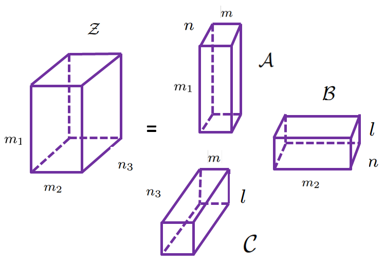
Figure 1. The image fusion is displayed in the left image, and the tensor triple decomposition structure is shown in the right.

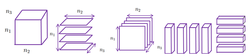
Figure 2. Slices and fibers of tensor $\mathcal{A}$. From left to right are horizontal slices $\mathcal{A}_{i,:,:}$, frontal slices $\mathcal{A}_{:,:,k}$, column fibers $\mathcal{A}_{i,:,k}$, and row fibers $\mathcal{A}_{:,j,k}$.

3. The tensor triple decomposition (TTD) model for HSI-MSI fusion

Hyperspectral and multispectral image fusion problems have been investigated with the aid of various tensor decompositions in recent years. Define $\mathcal{Y}_{h}\in\mathbb{R}^{n_{1}\times n_{2}\times n_{3}}$, $\mathcal{Y}_{m}\in\mathbb{R}^{m_{1}\times m_{2}\times m_{3}}$ and $\mathcal{Z}\in\mathbb{R}^{m_{1}\times m_{2}\times n_{3}}$ as hyperspectral image (HSI), multispectral image (MSI) and super-resolution image (SRI) respectively. Here the first two indices $n_{1}$ and $n_{2}$ or $m_{1}$ and $m_{2}$ denote the spatial dimensions. The third index $n_{3}$ or $m_{3}$ indicate the number of spectral bands. Usually, the MSI contains more spatial information than the HSI, that is $m_{1}\gg n_{1},m_{2}\gg n_{2}.$ The HSI has more spectral bands than MSI, which means $n_{3}\gg m_{3}.$ Our target is to find the SRI that possesses the high spectral resolution of HSI and the spatial resolution of the MSI, i.e. a super-resolution image.

3.1. The links among SRI, HSI and MSI

Let the mode-$3$ matricization of $\mathcal{Y}_{h}$, $\mathcal{Y}_{m}$ and $\mathcal{Z}$ be $(Y_{h})_{(3)}\in\mathbb{R}^{n_{1}n_{2}\times n_{3}},(Y_{m})_{(3)}\in\mathbb{R}^{m_{1}m_{2}\times m_{3}}$ and $Z_{(3)}\in\mathbb{R}^{m_{1}m_{2}\times n_{3}}.$ The key point which helps us to construct the relationship among SRI, HSI and MSI is that there exist two linear operators $P_{h}\in\mathbb{R}^{n_{1}n_{2}\times m_{1}m_{2}}$ and $P_{3}\in\mathbb{R}^{m_{3}\times n_{3}}$ such that $(Y_{h})_{(3)}=P_{h}Z_{(3)}$ and $(Y_{m})_{(3)}=Z_{(3)}P_{3}^{T}$ [20]. Thus we have

$$\mathcal{Y}_{h}(:,:,k)=P_{1}\mathcal{Z}(:,:,k)P_{2}^{T},\quad\text{for}\ k=1,\ldots,n_{3},$$ (5)

where $P_{1}\in\mathbb{R}^{n_{1}\times m_{1}}$, $P_{2}\in\mathbb{R}^{n_{2}\times m_{2}}$ and $P_{2}\otimes P_{1}=P_{h}.$ We also have

$$\mathcal{Y}_{m}(i,j,:)={P}_{3}\mathcal{Z}(i,j,:),\quad\text{for}\ i=1,\ldots,m_{1},\ j=1,\ldots,m_{2},$$ (6)

where $\mathcal{Z}(i,j,:)\in\mathbb{R}^{n_{3}}$ represents a fiber of $\mathcal{Z}$ and $\mathcal{Y}_{m}(i,j,:)\in\mathbb{R}^{m_{3}}$ is a fiber of $\mathcal{Y}_{m}$ respectively. Thus $\mathcal{Y}_{h}$, $\mathcal{Y}_{m}$ can be rewritten as

$$\mathcal{Y}_{h}=\mathcal{Z}\times_{1}{P}_{1}\times_{2}{P}_{2},\quad\mathcal{Y}_{m}=\mathcal{Z}\times_{3}{P}_{3}.$$ (7)

Equations $(\ref{3})$ and $(\ref{4})$ also are known as the spatial and spectral degradation processes of $\mathcal{Z}.$ The matrices $P_{1}$, $P_{2}$ respectively describe the downsampling and blurring of the spatial degradation process. Downsampling is considered as linear compression, while blurring describes a linear mixing of neighbouring pixels under a specific kernel in both the row and column dimensions. The matrix ${P}_{3}$ is usually modeled as a band-selection matrix that selects the common spectral bands of the SRI and MSI.

Based on the correlation of spatial and spectral information in hyperspectral and multispectral images, various low rank tensor decomposition models are established to study the problem. For example, suppose $\mathcal{Z}$ is decomposed by Canonical Polyadic decomposition into the sum of several rank-$1$ tensors, which is represented as $\mathcal{Z}=\llbracket{A},{B},{C}\rrbracket.$ The HSI-MSI fusion model [20] is denoted as $\mathcal{Y}_{h}=\llbracket{P}_{1}{A},{P}_{2}{B},{C}\rrbracket$ and $\mathcal{Y}_{m}=\llbracket{A},{B},{P}_{3}{C}\rrbracket$. Besides, Tucker decomposition is considered [44] and it is expressed as $\mathcal{Y}_{h}=\mathcal{C}\times_{1}\left({P}_{1}{A}\right)\times_{2}\left({P}_{2}{B}\right)\times_{3}{C}$ and $\mathcal{Y}_{m}=\mathcal{C}\times_{1}{A}\times_{2}{B}\times_{3}\left({P}_{3}{C}\right)$.

3.2. The new model for HSI-MSI fusion

In [29], Qi et al. proposed a new tensor decomposition, named tensor triple decomposition, which can effectively express the original tensor information by three low rank tensors. Therefore, we establish the hyperspectral and multispectral image fusion model by low rank tensor triple decomposition.

First, we introduce the tensor triple decomposition in detail. Tensor triple decomposition of a third-order $\mathcal{Z}\in\mathbb{Re}^{m_{1}\times m_{2}\times n_{3}}$ representing the target SRI takes the following form

$$\mathcal{Z}=\mathcal{A}\mathcal{B}\mathcal{C},$$ (8)

where $\mathcal{A}\in\mathbb{Re}^{m_{1}\times m\times n}$, $\mathcal{B}\in\mathbb{Re}^{l\times m_{2}\times n}$ and $\mathcal{C}\in\mathbb{Re}^{l\times m\times n_{3}}.$ It can also be denoted as $\mathcal{Z}=\llbracket\mathcal{A},\mathcal{B},\mathcal{C}\rrbracket$ with its entries

$$(\llbracket\mathcal{A},\mathcal{B},\mathcal{C}\rrbracket)_{ijk}=\sum_{t=1}^{l}\sum_{p=1}^{m}\sum_{q=1}^{n}a_{ipq}b_{tjq}c_{tpk},$$ (9)

for $i=1,\ldots,m_{1}$, $j=1,\ldots,m_{2}$, and $k=1,\ldots,n_{3}.$ The smallest value of $r$ such that (9) holds is called the triple rank of $\mathcal{Z}$ and denoted as $\operatorname{rank}(\mathcal{Z})=r$. If $l=m=n=r$, equation (8) is called low rank triple decomposition of $\mathcal{Z}$, where $r\leq\operatorname{mid}\left\{m_{1},m_{2},n_{3}\right\}$ and mid represents the larger number in the middle [29, 11]. In particular, according to [11, Theorem 2.2], triple decomposition satisfies the following equations

$$\begin{split}Z_{m_{1}\times m_{2}n_{3}}&=A_{m_{1}\times nm}\left(E_{m}\otimes B_{n\times m_{2}l}\right)\left(C_{lm\times n_{3}}\otimes E_{m_{2}}\right),\\ Z_{m_{2}\times n_{3}m_{1}}&=B_{m_{2}\times ln}\left(E_{n}\otimes C_{l\times n_{3}m}\right)\left(A_{mn\times m_{1}}\otimes E_{n_{3}}\right),\\ Z_{n_{3}\times m_{2}m_{1}}&=C_{n_{3}\times lm}\left(E_{m}\otimes B_{l\times m_{2}n}\right)\left(A_{nm\times m_{1}}\otimes E_{m_{2}}\right),\end{split}$$ (10)

where $E$ is an identity matrix with a proper size.

Next, we propose a new model with the help of low rank tensor triple decomposition. Assume $\mathcal{A}$, $\mathcal{B}$ and $\mathcal{C}$ are the low rank triple decomposition tensors of tensor $\mathcal{Z}.$ For the connection (7), we have

$$\mathcal{Y}_{h}=\llbracket\mathcal{A}\times_{1}{P_{1}},\mathcal{B}\times_{2}{P_{2}},\mathcal{C}\rrbracket\quad\text{and}\quad\mathcal{Y}_{m}=\llbracket\mathcal{A},\mathcal{B},\mathcal{C}\times_{3}{P_{3}}\rrbracket.$$ (11)

Since the best low rank approximation problem of tensors may be ill-posed, we add the Tikhonov regularization term and get the following optimization model

$$\begin{split}\min_{\mathcal{A},\mathcal{B},\mathcal{C}}f(\mathcal{A},\mathcal{B},\mathcal{C}):&=\left\|\mathcal{Y}_{h}-\llbracket\mathcal{A}\times_{1}{P_{1}},\mathcal{B}\times_{2}{P_{2}},\mathcal{C}\rrbracket\right\|_{F}^{2}+\left\|\mathcal{Y}_{m}-\llbracket\mathcal{A},\mathcal{B},\mathcal{C}\times_{3}{P_{3}}\rrbracket\right\|_{F}^{2}\\ &\quad+\mu\left(\|\mathcal{A}\|_{F}^{2}+\|\mathcal{B}\|_{F}^{2}+\|\mathcal{C}\|_{F}^{2}\right),\end{split}$$ (12)

where $\mu$ is regularization parameter. Thus, we employ the optimization model (12) to obtain the triple decomposition tensors $\mathcal{A},\mathcal{B}$ and $\mathcal{C}$ and to produce the super-resolution image by $\mathcal{Z}=\llbracket\mathcal{A},\mathcal{B},\mathcal{C}\rrbracket$.

4. The L-BFGS algorithm for solving the TTD model

In this section, we focus on numerical approaches for computing a first-order stationary point of the optimization problem (12). Since the limited memory BFGS (L-BFGS) algorithm [21] is powerful for large scale nonlinear unconstrained optimization, we apply it to produce a search direction and consider using inexact line search techniques to update the iteration step size. In the computaion process, we either matricize or vectorize the tensor variable to get the gradient of the objective function. For convenience, we demonstrate the algorithm and its convergence analysis for

$$\mathbf{x}:=\left(\begin{array}[]{l}\mathbf{a}_{m_{1}rr}\\ \mathbf{b}_{m_{2}rr}\\ \mathbf{c}_{n_{3}rr}\end{array}\right)=\left(\begin{array}[]{c}A_{m_{1}rr\times 1}\\ B_{m_{2}rr\times 1}\\ C_{n_{3}rr\times 1}\end{array}\right).$$ (13)

4.1. Limited memory BFGS algorithm

BFGS is a quasi-Newton method which updates the approximation of the inverse of a Hessian iteratively. In the current iteration $k$, it constructs an approximation matrix $H_{k}$ to estimate the inverse of Hessian of $f(\mathbf{x})$. The gradient of $f(\mathbf{x})$ is defined as $\mathbf{g(x)}.$ At the beginning, we introduce the basic BFGS update. Let

$$\quad\mathbf{y}_{k}=\nabla f\left(\mathbf{x}_{k+1}\right)-\nabla f\left(\mathbf{x}_{k}\right),\quad\mathbf{s}_{k}=\mathbf{x}_{k+1}-\mathbf{x}_{k},\quad V_{k}=I-\rho_{k}\mathbf{y}_{k}\mathbf{s}_{k}^{\top},$$ (14)

and

$$\begin{aligned} \hfil\displaystyle\begin{split}\rho_{k}=\left\{\begin{array}[]{ll}\frac{1}{\mathbf{y}_{k}^{\top}\mathbf{s}_{k}},&\text{ if }\mathbf{y}_{k}^{\top}\mathbf{s}_{k}\geq\epsilon\\ 0,&\text{ otherwise }\end{array}\right.\end{split}\end{aligned},$$ (15)

where $I$ is an identity matrix, $\top$ represents transposition and $\epsilon\in(0,1)$ is a small positive constant. The matrix $H_{k}$ is updated by

$$H_{k+1}=V_{k}^{\top}H_{k}V_{k}+\rho_{k}\mathbf{s}_{k}\mathbf{s}_{k}^{\top}.$$ (16)

To deal with large-scale optimization problems, Liu and Nocedal [21] proposed the L-BFGS algorithm that implements BFGS updates in an economical manner. Given a constant $l.$ When $k\geq l,$ only information of $l$ matrices $H_{k-1},H_{k-2},\ldots,H_{k-l}$ are used to calculate the matrix $H_{k}$ by the following recursive form

$${H_{k}}=V_{k-m}^{\top}H_{k-m}V_{k-m}+\rho_{k-m}\mathbf{s}_{k-m}\mathbf{s}_{k-m}^{\top},\quad\text{ for }m=1,2,\ldots,l.$$ (17)

In order to save memory, the initial matrix $H_{k-l}$ is replaced by

$$H_{k}^{(0)}=\gamma_{k}{I}.$$ (18)

Here $\gamma_{k}>0$ is usually determined by the Barzilai-Borwein method [3] as follows

$$\gamma_{k}^{\mathrm{BB}1}=\frac{\mathbf{y}_{k}^{\top}\mathbf{s}_{k}}{\left\|\mathbf{y}_{k}\right\|^{2}}\quad\text{ and }\quad\gamma_{k}^{\mathrm{BB}2}=\frac{\left\|\mathbf{s}_{k}\right\|^{2}}{\mathbf{y}_{k}^{\top}\mathbf{s}_{k}}.$$ (19)

If $l\geq k$, $H_{k}$ is generated by the traditional BFGS method. The L-BFGS method can be implemented in an inexpensive two-loop recursion way which is shown in Algorithm 1.

The $\mathbf{p}_{k}=-H_{k}\mathbf{g}\left(\mathbf{x}_{k}\right)$ generated by L-BFGS is a gradient-related descent direction for $H_{k}$ beging a positive definite matrix, where the proof process is presented in Lemma B.2. Then we find a proper step size along the direction $\mathbf{p}_{k}$ that satisfies the Armijo condition. The computation method for the model (12) is obtained and we demonstrate it in Algorithm 2.

Algorithm 1 The two-loop recursion for L-BFGS [10, 21].

1:  $\mathbf{q}\leftarrow-\mathbf{g}\left(\mathbf{x}_{k}\right)$

2:  for  $i=k-1,k-2,\ldots,k-l$  do

3:     $\quad\alpha_{i}\leftarrow\rho_{i}\mathbf{s}_{i}^{\top}\mathbf{q}$

4:     $\quad\mathbf{q}\leftarrow\mathbf{q}-\alpha_{i}\mathbf{y}_{i}$

5:  end for

6:  for for $i=k-l,k-l+1,\ldots,k-1$ do

7:     $\quad\beta\leftarrow\rho_{i}\mathbf{y}_{i}^{\top}\mathbf{p}$

8:     $\quad\mathbf{p}\leftarrow\mathbf{p}+\mathbf{s}_{i}\left(\alpha_{i}-\beta\right)$

9:  end for

10:  Stop with result $\mathbf{p}=-H_{k}\mathbf{g}\left(\mathbf{x}_{k}\right)$.

Algorithm 2 Low rank triple decomposition for obtaining super-resolution image (TTDSR).

1:  Choose constant $r$ and an initial iterate $\mathbf{x}_{0}\in\mathbb{Re}^{m_{1}rr+m_{2}rr+n_{3}rr}$. Select parameters ${l}>0$, $\beta\in\left(0,1\right)$, and $\sigma\in\left(0,1\right)$. Compute $f_{0}=f\left(\mathbf{x}_{0}\right)$ and $\mathbf{g}_{0}=\nabla f\left(\mathbf{x}_{0}\right)$. Set $k\leftarrow 0.$

2:  while the sequence of iterates does not converge do

3:     Generate $\mathbf{p}_{k}=-H_{k}\mathbf{g}\left(\mathbf{x}_{k}\right)$ by Algorithm 1.

4:     Choose the smallest nonnegative integer $\omega$ such that the step size $\alpha=\beta^{\omega}$ satisfies

$$f\left(\mathbf{x}_{k}+\alpha\mathbf{p}_{k}\right)\leq f\left(\mathbf{x}_{k}\right)+\sigma\alpha\mathbf{p}_{k}^{\top}\mathbf{g}_{k}.$$ (20)

5:     Let $\alpha_{k}=\beta^{\omega}$ and update the new iterate $\mathbf{x}_{k+1}=\mathbf{x}_{k}+\alpha_{k}\mathbf{p}_{k}$.

6:     Compute $f_{k+1}=f\left(\mathbf{x}_{k+1}\right)$ and $\mathbf{g}_{k+1}=\nabla f\left(\mathbf{x}_{k+1}\right)$.

7:     Compute $\mathbf{y}_{k}$, $\mathbf{s}_{k}$ and $\mathbf{\rho}_{k}$ by (14) and (15), respectively.

8:     $k\leftarrow k+1.$

9:  end while

4.2. Gradient calculation

At each iteration in Algorithm 2, we need to compute the gradient of the objective function. The gradient can be calculated via reshaping the tensor variable into vector or matrix form. For small scale problems, the gradient is easier to obtain when the the tensor variable is turned into a vector than into a matrix, while for large scale problems, the gradient in vector form always leads to insufficient memory in the computation process. In this subsection, we derive the matrix form of the gradient and the vector form $\nabla f$ is given in the Appendix A.

Denote $\mathcal{H}=\mathcal{A}\times_{1}P_{1}\in\mathbb{Re}^{n_{1}\times m\times n}$, $\mathcal{K}=\mathcal{B}\times_{2}P_{2}\in\mathbb{Re}^{l\times n_{2}\times n}$, and $\mathcal{G}=\mathcal{C}\times_{3}P_{3}\in\mathbb{Re}^{l\times m\times m_{3}}.$ According to (10) and (11), we get the following equations

$$\left(Y_{h}\right)_{n_{1}\times{n_{2}{n_{3}}}} =P_{n_{1}\times m_{1}}A_{m_{1}\times nm}\left(E_{m}\otimes K_{n\times n_{2}l}\right)\left(C_{lm\times n_{3}}\otimes E_{n_{2}}\right),$$ (21)

$$\left(Y_{h}\right)_{n_{2}\times{{n_{3}n_{1}}}} =P_{n_{2}\times m_{2}}B_{m_{2}\times ln}\left(E_{n}\otimes C_{l\times n_{3}m}\right)\left(H_{mn\times n_{1}}\otimes E_{n_{3}}\right),$$ (22)

$$\left(Y_{h}\right)_{n_{3}\times{{n_{2}n_{1}}}} =C_{n_{3}\times lm}\left(E_{m}\otimes K_{l\times n_{2}n}\right)\left(H_{nm\times n_{1}}\otimes E_{n_{2}}\right),$$ (23)

$$\left(Y_{m}\right)_{m_{1}\times{{m_{2}m_{3}}}} =A_{m_{1}\times nm}\left(E_{m}\otimes B_{n\times m_{2}l}\right)\left(G_{lm\times m_{3}}\otimes E_{m_{2}}\right),$$ (24)

$$\left(Y_{m}\right)_{m_{2}\times{{m_{3}m_{1}}}} =B_{m_{2}\times ln}\left(E_{n}\otimes G_{l\times m_{3}m}\right)\left(A_{mn\times m_{1}}\otimes E_{m_{3}}\right),$$ (25)

$$\left(Y_{m}\right)_{m_{3}\times{{m_{2}m_{1}}}} =P_{m_{3}\times n_{3}}C_{n_{3}\times lm}\left(E_{m}\otimes B_{l\times m_{2}n}\right)\left(A_{nm\times m_{1}}\otimes E_{m_{2}}\right).$$ (26)

Define ${P}_{2}{B}_{{m}_{2}\times{ln}}={K}_{{n}_{2}\times ln}$ and ${P}_{3}{C}_{{n}_{3}\times lm}={G}_{{m}_{3}\times{lm}}.$ The function $f(\mathbf{x})$ in (12) is transformed into the objective function of matrix variables ${A_{m_{1}\times nm}}$, ${B_{m_{2}\times ln}}$ and ${C_{n_{3}\times lm}}$ as follows

$$\begin{split}f(A,B,C)&=\left\|P_{1}A_{m_{1}\times nm}\left(E_{m}\otimes K_{n\times n_{2}l}\right)\left(C_{n_{3}\times lm}^{T}\otimes E_{n_{2}}\right)-\left(Y_{h}\right)_{n_{1}\times n_{2}n_{3}}\right\|_{F}^{2}\\ &+\left\|A_{m_{1}\times nm}\left(E_{m}\otimes B_{n\times m_{2}L}\right)\left(\left(P_{3}C_{n_{3}\times lm}\right)^{T}\otimes E_{m_{2}}\right)-\left(Y_{m}\right)_{m_{1}\times m_{2}m_{3}}\right\|_{F}^{2}\\ &+\mu\left(\left\|{A}_{{m}_{1}\times{nm}}\right\|_{{F}}^{2}+\left\|{B}_{{m}_{2}\times{ln}}\right\|_{{F}}^{2}+\left\|{C}_{{n}_{3}\times{lm}}\right\|_{{F}}^{2}\right),\end{split}$$ (27)

$$\begin{split}f(A,B,C)&=\left\|P_{2}B_{m_{2}\times ln}\left(E_{n}\otimes C_{l\times n_{3}m}\right)\left(\left(P_{1}{A_{m_{1}\times mn}}\right)^{T}\otimes E_{n_{3}}\right)-\left(Y_{h}\right)_{n_{2}\times n_{3}n_{1}}\right\|_{F}^{2}\\ &+\left\|B_{m_{2}\times ln}\left(E_{n}\otimes G_{l\times m_{3}m}\right)\left(\left(A_{m_{1}\times mn}\right)^{T}\otimes E_{m_{3}}\right)-\left(Y_{m}\right)_{m_{2}\times m_{3}m_{1}}\right\|_{F}^{2}\\ &+\mu\left(\left\|{A}_{{m}_{1}\times{nm}}\right\|_{{F}}^{2}+\left\|{B}_{{m}_{2}\times{ln}}\right\|_{{F}}^{2}+\left\|{C}_{{n}_{3}\times{lm}}\right\|_{{F}}^{2}\right),\end{split}$$ (28)

$$\begin{split}f(A,B,C)&=\left\|C_{n_{3}\times lm}\left(E_{m}\otimes K_{l\times n_{2}n}\right)\left(\left(P_{1}{A_{m_{1}\times mn}}\right)^{T}\otimes E_{n_{2}}\right)-\left(Y_{h}\right)_{n_{3}\times n_{2}n_{1}}\right\|_{F}^{2}\\ &+\left\|P_{3}C_{n_{3}\times lm}\left(E_{m}\otimes B_{l\times m_{2}n}\right)\left(\left(A_{m_{1}\times nm}\right)^{T}\otimes E_{m_{2}}\right)-\left(Y_{m}\right)_{m_{3}\times m_{2}m_{1}}\right\|_{F}^{2}\\ &+\mu\left(\left\|{A}_{{m}_{1}\times{nm}}\right\|_{F}^{2}+\left\|{B}_{{m}_{2}\times{ln}}\right\|_{{F}}^{2}+\left\|{C}_{{n}_{3}\times{lm}}\right\|_{{F}}^{2}\right).\end{split}$$ (29)

For any matrix $X,$ we have $\|X\|_{F}^{2}=tr(X^{\top}X).$ Therefore we review the derivatives of some useful trace functions with respect to $X:$

$$\normalsize\begin{split}&\dfrac{\partial tr(AXBX^{T}C)}{\partial X}=A^{T}C^{T}XB^{T}+CAXB,\quad\quad\dfrac{\partial tr(AX^{T}B)}{\partial X}=BA,\quad\\ &\dfrac{\partial tr(ABA^{T})}{\partial A}=A(B+B^{T}),\quad\quad\quad\quad\quad\quad\quad\quad\quad\dfrac{\partial tr(BA^{T})}{\partial A}=B,\quad\\ &\dfrac{\partial tr(AXB)}{\partial X}=A^{T}B^{T},\qquad\qquad\qquad\qquad\qquad\quad\quad\dfrac{\partial tr(AB)}{\partial A}=B^{T}.\quad\end{split}$$ (30)

For simplicity, we denote

$${E_{1}} =\left(E_{m}\otimes B_{n\times m_{2}l}\right)\left(\left(P_{3}C_{n_{3}\times lm}\right)^{T}\otimes E_{m_{2}}\right), {D_{1}} =\left(E_{m}\otimes K_{n\times n_{2}l}\right)\left(C_{n_{3}\times lm}^{T}\otimes E_{n_{2}}\right),$$

$${F_{1}} =\left(E_{n}\otimes C_{l\times n_{3}m}\right)\left(\left(P_{1}{A_{m_{1}\times mn}}\right)^{T}\otimes E_{n_{3}}\right), {G_{1}} =\left(E_{n}\otimes G_{l\times m_{3}m}\right)\left(A_{m_{1}\times mn}^{T}\otimes E_{m_{3}}\right),$$

$$H_{1} =\left(E_{m}\otimes K_{l\times n_{2}n}\right)\left(\left(P_{1}{A_{m_{1}\times mn}}\right)^{T}\otimes E_{n_{2}}\right), K_{1} =\left(E_{m}\otimes B_{l\times m_{2}n}\right)\left(A_{m_{1}\times nm}^{T}\otimes E_{m_{2}}\right).$$

Thus, the partial derivatives with respect to $A,$ $B,$ and $C$ are

$$\begin{split}\dfrac{\partial f({A},{B},{C})}{\partial{A}}=&\dfrac{\partial\left(\left\|{P_{1}}{A}{D_{1}}-{Y_{h}}\right\|_{F}^{2}+\left\|{A}{E_{1}}-{Y_{m}}\right\|_{F}^{2}+\mu\left(\left\|{A}\right\|_{{F}}^{2}+\left\|{B}\right\|_{{F}}^{2}+\left\|{C}\right\|_{{F}}^{2}\right)\right)}{\partial{A}}\\ \vspace{1.5ex}=&\dfrac{\partial tr\left(\langle{P_{1}}{A}{D_{1}}-{Y_{h}},{P_{1}}{A}{D_{1}}-{Y_{h}}\rangle+\langle{A}{E_{1}}-{Y_{m}},{A}{E_{1}}-{Y_{m}}\rangle\right)}{\partial{A}}+2\mu{A}\\ =&\dfrac{\partial tr\left({P_{1}}{A}{D_{1}}{D_{1}^{T}}{A^{T}}{P_{1}^{T}}-{P_{1}}{A}{D_{1}}{Y_{h}^{T}}-{Y_{h}}{D_{1}^{T}}{A^{T}}{P_{1}^{T}}-{Y_{h}}{Y_{h}^{T}}\right)}{\partial{A}}\\ +&\dfrac{\partial tr\left({A}{E_{1}}{E_{1}^{T}}{A^{T}}-{A}{E_{1}}{Y_{m}^{T}}-{Y_{m}}{E_{1}^{T}}{A^{T}}+{Y_{m}^{T}}{Y_{m}}\right)}{{\partial{A}}}+2\mu{A}\\ =&2\left({P_{1}^{T}}{P_{1}}A{D_{1}}{D_{1}^{T}}-{P_{1}^{T}}{Y_{h}}{D_{1}^{T}}+{A}{E_{1}}{E_{1}^{T}}-{Y_{m}}{E_{1}^{T}}+\mu{A}\right),\end{split}$$ (31)

$$\begin{split}\dfrac{\partial f({A},{B},{C})}{\partial{B}}=&\dfrac{\partial\left(\left\|{P_{2}}{B}{F_{1}}-{Y_{h}}\right\|_{F}^{2}+\left\|{B}{G_{1}}-{Y_{m}}\right\|_{F}^{2}+\mu\left(\left\|{A}\right\|_{{F}}^{2}+\left\|{B}\right\|_{{F}}^{2}+\left\|{C}\right\|_{{F}}^{2}\right)\right)}{\partial{B}}\\ =&\dfrac{\partial tr\left(\langle{P_{2}}{B}{F_{1}}-{Y_{h}},{P_{2}}{B}{F_{1}}-{Y_{h}}\rangle+\langle{B}{G_{1}}-{Y_{m}},{B}{G_{1}}-{Y_{m}}\rangle\right)}{\partial{B}}+2\mu{B}\\ =&\dfrac{\partial tr\left({P_{2}}{B}{F_{1}}{F_{1}^{T}}{B^{T}}{P_{2}^{T}}-{P_{2}}{B}{F_{1}}{Y_{h}^{T}}-{Y_{h}}{F_{1}^{T}}{B^{T}}{P_{2}^{T}}-{Y_{h}}{Y_{h}^{T}}\right)}{\partial{B}}\\ +&\dfrac{\partial tr\left({B}{G_{1}}{G_{1}^{T}}{B^{T}}-{B}{G_{1}}{Y_{m}^{T}}-{Y_{m}}{G_{1}^{T}}{B^{T}}+{Y_{m}^{T}}{Y_{m}}\right)}{{\partial{B}}}+2\mu{B}\\ =&2\left({P_{2}^{T}}{P_{2}}B{F_{1}}{F_{1}^{T}}-{P_{2}^{T}}{Y_{h}}{F_{1}^{T}}+{B}{G_{1}}{G_{1}^{T}}-{Y_{m}}{G_{1}^{T}}+\mu{B}\right),\end{split}$$ (32)

$$\begin{split}\dfrac{\partial f({A},{B},{C})}{\partial{C}}=&\dfrac{\partial\left(\left\|{C}{H_{1}}-{Y_{h}}\right\|_{F}^{2}+\left\|{P_{3}}{C}{K_{1}}-{Y_{m}}\right\|_{F}^{2}+\mu\left(\left\|{A}\right\|_{{F}}^{2}+\left\|{B}\right\|_{{F}}^{2}+\left\|{C}\right\|_{{F}}^{2}\right)\right)}{\partial{C}}\\ =&\dfrac{\partial tr\left(\langle{C}{H_{1}}-{Y_{h}},{C}{H_{1}}-{Y_{h}}\rangle+\langle{P_{3}}{C}{K_{1}}-{Y_{m}},P_{3}{C}{K_{1}}-{Y_{m}}\rangle\right)}{\partial{C}}+2\mu{C}\\ =&\dfrac{\partial tr\left({C}{H_{1}}{H_{1}^{T}}{C^{T}}-{C}{H_{1}}{Y_{h}^{T}}-{Y_{h}}{H_{1}^{T}}{C^{T}}+{Y_{h}^{T}}{Y_{h}}\right)}{\partial{C}}\\ +&\dfrac{\partial tr\left({P_{3}}{C}{K_{1}}{K_{1}^{T}}{C^{T}}{P_{3}^{T}}-{P_{3}}{C}{K_{1}}{Y_{m}^{T}}-{Y_{m}}{K_{1}^{T}}{C^{T}}{P_{3}^{T}}-{Y_{m}}{Y_{m}^{T}}\right)}{\partial{C}}+2\mu{C}\\ =&2\left({C}{H_{1}}{H_{1}^{T}}-{Y_{h}}{H_{1}^{T}}+{P_{3}^{T}}{P_{3}}C{K_{1}}{K_{1}^{T}}-{P_{3}^{T}}{Y_{m}}{K_{1}^{T}}+\mu{C}\right).\end{split}$$ (33)

5. Convergence analysis

In this section, we analyze the convergence of $\|\mathbf{g}(\mathbf{x})\|$ and show that our proposed method produces a globally convergent iteration.

Lemma 5.1.

There exists a positive number $M$ such that

$$\lvert f(\mathbf{x})\rvert\leq M,\|\mathbf{g}(\mathbf{x})\|\leq M,\|H(\mathbf{x})\|\leq M.$$ (34)

Proof.

Because $\mathbf{p}_{k}=-H_{k}\mathbf{g}\left(\mathbf{x}_{k}\right)$ generated by L-BFGS is a gradient-related descent direction. There exists a positive number satisfies the Armijo condition in (20) and the sequence of objective function value $\left\{f\left(\mathbf{x}_{k}\right)\right\}$ decreases monotonically. Since the value of the objective function $f\left(\mathbf{x}\right)$ in (12) is nonnegative, $f\left(\mathbf{x}\right)$ is bounded, i.e. $0\leq f(\mathbf{x})\leq M$ holds.

The regularization term $\mu\left(\|\mathcal{A}\|_{F}^{2}+\|\mathcal{B}\|_{F}^{2}+\|\mathcal{C}\|_{F}^{2}\right)$ in the objective function indicates that the sequence $\left\{\mathbf{x}_{k}\right\}$ is bounded. Because $\mathbf{g}\left(\mathbf{x}\right)$ is a linear function of $\mathbf{x}$, $\|\mathbf{g}(\mathbf{x})\|$ is also bounded. The proof of the boundedness of $H(\mathbf{x})$ is shown in Appendix B. Thus, we get Lemma 5.1. ∎

Furthermore, we have the following Lemma 5.2.

Lemma 5.2.

There exist constants $C_{m}$ and $C_{M}$ satisfy $0<C_{m}\leq 1\leq C_{M}$,

$$\mathbf{p}_{k}^{\top}\mathbf{g}\left(\mathbf{x}_{k}\right)\leq-C_{m}\left\|\mathbf{g}\left(\mathbf{x}_{k}\right)\right\|^{2}\quad\text{ and }\quad\left\|\mathbf{p}_{k}\right\|\leq C_{M}\left\|\mathbf{g}\left(\mathbf{x}_{k}\right)\right\|.$$ (35)

Proof.

The proof can be found in the Appendix B. ∎

Because of boundedness and monotonicity of $\{f\left(\mathbf{x}_{k}\right)\}$, the sequence of function value converges. The conclusion is given in Theorem 5.3.

Theorem 5.3.

Assume that Algorithm 2 generates an infinite sequence of function values $\left\{f\left(\mathbf{x}_{k}\right)\right\}$. Then, there exists a constant ${f}_{*}$ such that

$$\lim_{k\rightarrow\infty}f\left(\mathbf{x}_{k}\right)=f_{*}.$$ (36)

Next, we prove that every accumulation point of iterates $\{\mathbf{x}_{k}\}$ is a first-order stationary point. At last, by utilizing the Kurdyka-$\L$ojasiewicz property [2], we show that the sequence of iterates $\left\{\mathbf{x}_{k}\right\}$ is also convergent. The following lemma means that the step size is lower bounded.

Lemma 5.4.

There exists a constant $\alpha_{\min}>0$ such that

$$\alpha_{k}\geq\alpha_{\min}>0,\quad\quad\forall k\in\mathbf{N}^{+}.$$ (37)

Proof.

Let $0<\alpha\leq\tilde{\alpha}=\frac{(1-\sigma)C_{m}}{\frac{1}{2}MC_{M}^{2}}$. From Lemma 5.2, for $\alpha\in(0,\tilde{\alpha}]$, it yields that

$$\begin{split}\alpha\mathbf{p}_{k}^{T}\mathbf{g}_{k}+\frac{1}{2}M\alpha^{2}\left\|\mathbf{p}_{k}\right\|^{2}-\sigma\alpha\mathbf{p}_{k}^{T}\mathbf{g}_{k}&=(1-\sigma)\alpha\mathbf{p}_{k}^{T}\mathbf{g}_{k}+\frac{1}{2}M\alpha^{2}\left\|\mathbf{p}_{k}\right\|^{2}\\ &\leq(1-\sigma)\alpha(-C_{m}\left\|\mathbf{g}\left(\mathbf{x}_{k}\right)\right\|^{2})+\frac{1}{2}M\alpha^{2}C_{M}^{2}\left\|\mathbf{g}_{k}\right\|^{2}\\ &\leq 0.\end{split}$$ (38)

From Taylor’s mean value theorem and $\mathbf{x}_{k+1}(\alpha)=\mathbf{x}_{k}+\alpha\mathbf{p}_{k}$, we have

$$f\left(\mathbf{x}_{k+1}(\alpha)\right)-f\left(\mathbf{x}_{k}\right) \leq\mathbf{g}_{k}^{T}\left(\mathbf{x}_{k+1}(\alpha)-\mathbf{x}_{k}\right)+\frac{1}{2}M\left\|\mathbf{x}_{k+1}(\alpha)-\mathbf{x}_{k}\right\|^{2}$$ (39)

$$=\alpha\mathbf{p}_{k}^{T}\mathbf{g}_{k}+\frac{1}{2}M\alpha^{2}\left\|\mathbf{p}_{k}\right\|^{2}$$

$$\leq\sigma\alpha\mathbf{p}_{k}^{T}\mathbf{g}_{k},$$

where the last inequality is valid owing to (38). The rule of inexact line search indicates $\alpha_{k}\geq\alpha_{\min}=\tilde{\alpha}\beta.$ Hence, we find out a lower bound on the step size $\alpha$. ∎

The following theorem proves that every accumulation point of iterates $\left\{\mathbf{x}_{k}\right\}$ is a first-order stationary point.

Theorem 5.5.

Suppose that Algorithm 2 generates an infinite sequence of iterates $\left\{\mathbf{x}_{k}\right\}$. Then,

$$\lim_{k\rightarrow\infty}\left\|\mathbf{g}\left(\mathbf{x}_{k}\right)\right\|=0.$$ (40)

Proof.

From Lemma 5.2 and (20), we get

$$f\left(\mathbf{x}_{k}\right)-f\left(\mathbf{x}_{k+1}\right)\geq-\sigma\alpha_{k}\mathbf{p}_{k}^{\top}\mathbf{g}\left(\mathbf{x}_{k}\right)\geq\sigma\alpha_{k}C_{m}\left\|\mathbf{g}\left(\mathbf{x}_{k}\right)\right\|^{2}.$$ (41)

The functional series $\sum_{k=1}^{\infty}\left[f\left(\mathbf{x}_{k}\right)-f\left(\mathbf{x}_{k+1}\right)\right]$ satisfies

$$\begin{split}2M\geq f\left(\mathbf{x}_{1}\right)-f_{*}&=\sum_{k=1}^{\infty}\left[f\left(\mathbf{x}_{k}\right)-f\left(\mathbf{x}_{k+1}\right)\right]\\ &\geq\sum_{k=1}^{\infty}\sigma\alpha_{k}C_{m}\left\|\mathbf{g}\left(\mathbf{x}_{k}\right)\right\|^{2}\\ &\geq\sum_{k=1}^{\infty}\sigma\alpha_{\min}C_{m}\left\|\mathbf{g}\left(\mathbf{x}_{k}\right)\right\|^{2}.\end{split}$$ (42)

That is to say,

$$\sum_{k=1}^{\infty}\left\|\mathbf{g}\left(\mathbf{x}_{k}\right)\right\|^{2}\leq\frac{2M}{\sigma\alpha_{\min}C_{m}}<+\infty.$$ (43)

Hence, $\left\|\mathbf{g}\left(\mathbf{x}_{k}\right)\right\|$ converges to zero. ∎

Analysis of proximal methods for nonconvex and nonsmooth optimization frequently uses the Kurdyka- $\L$ojasiewicz (KL) property [2]. Since the objective function $f(\mathbf{x})$ is a polynomial and the KL property below holds, we use the KL property to prove the convergence of algorithm.

Proposition 5.6.

(Kurdyka-$\L$ojasiewicz (KL) property) Suppose that $\mathbf{x}_{*}$ is a stationary point of $f(\mathbf{x})$. There is a neighborhood $\mathscr{U}$ of $\mathbf{x}_{*}$, an exponent $\theta\in[0,1)$ and a positive constant $K$ such that for all $\mathbf{x}\in\mathscr{U}$, the following inequality holds:

$$\left|f(\mathbf{x})-f\left(\mathbf{x}_{*}\right)\right|^{\theta}\leq K\|\mathbf{g}(\mathbf{x})\|.$$ (44)

In particular, we define $0^{0}\equiv 0$.

Lemma 5.7.

Suppose that $\mathbf{x}_{*}$ is a stationary point of $f(\mathbf{x})$ and $\mathscr{A}\left(\mathbf{x}_{*},\delta\right)=\{\mathbf{x}\in\left.\mathbb{R}^{n}:\left\|\mathbf{x}-\mathbf{x}_{*}\right\|\leq\delta\right\}\subseteq\mathscr{U}$ is a neighborhood of $\mathbf{x}_{*}.$ Let $\mathbf{x}_{1}$ be an initial point satisfying

$$\delta>\frac{C_{M}K}{\sigma C_{m}(1-\theta)}\left|f\left(\mathbf{x}_{1}\right)-f\left(\mathbf{x}_{*}\right)\right|^{1-\theta}+\left\|\mathbf{x}_{1}-\mathbf{x}_{*}\right\|.$$ (45)

Then, the following assertions hold:

$$\mathbf{x}_{k}\in\mathscr{A}\left(\mathbf{x}_{*},\delta\right),\quad k=1,2,\ldots$$ (46)

and

$$\sum_{k=1}^{\infty}\left\|\mathbf{x}_{k+1}-\mathbf{x}_{k}\right\|\leq\frac{C_{M}K}{\sigma C_{m}(1-\theta)}\left|f\left(\mathbf{x}_{1}\right)-f\left(\mathbf{x}_{*}\right)\right|^{1-\theta}.$$ (47)

Proof.

The theorem is proved by induction. Obviously, $\mathbf{x}_{1}\in\mathscr{A}\left(\mathbf{x}_{*},\delta\right)$. Now, we assume $\mathbf{x}_{i}\in\mathscr{A}\left(\mathbf{x}_{*},\delta\right)$ for all $i=1,\ldots,k$ and KL property holds at these points. Define a concave function

$$\phi(q)\equiv\frac{K}{1-\theta}\left|q-f\left(\mathbf{x}_{*}\right)\right|^{1-\theta}\quad and\quad q>f\left(\mathbf{x}_{*}\right).$$ (48)

Its derivative function is

$$\phi^{\prime}(q)=\frac{K}{\left|q-f\left(\mathbf{x}_{*}\right)\right|^{\theta}}.$$ (49)

For $i=1,\ldots,k$, the first-order condition of the concave function $\phi^{\prime}(q)$ at $f(\mathbf{x}_{i})$ is

$$\phi\left(f\left(\mathbf{x}_{i}\right)\right)-\phi\left(f\left(\mathbf{x}_{i+1}\right)\right) \geq\phi^{\prime}\left(f\left(\mathbf{x}_{i}\right)\right)\left(f\left(\mathbf{x}_{i}\right)-f\left(\mathbf{x}_{i+1}\right)\right)$$ (50)

$$=\frac{K}{\left|f\left(\mathbf{x}_{i}\right)-f\left(\mathbf{x}_{*}\right)\right|^{\theta}}\left(f\left(\mathbf{x}_{i}\right)-f\left(\mathbf{x}_{i+1}\right)\right).$$

The equation (50) and KL property mean

$$\phi\left(f\left(\mathbf{x}_{i}\right)\right)-\phi\left(f\left(\mathbf{x}_{i+1}\right)\right)\geq\frac{1}{\left\|\mathbf{g}\left(\mathbf{x}_{i}\right)\right\|}\left(f\left(\mathbf{x}_{i}\right)-f\left(\mathbf{x}_{i+1}\right)\right).$$ (51)

By Lemma 5.2 and (41), we have

$$\phi\left(f\left(\mathbf{x}_{i}\right)\right)-\phi\left(f\left(\mathbf{x}_{i+1}\right)\right)\geq\sigma\alpha_{i}C_{m}\left\|\mathbf{g}\left(\mathbf{x}_{i}\right)\right\|\geq\frac{\sigma C_{m}}{C_{M}}\left\|\mathbf{x}_{i+1}-\mathbf{x}_{i}\right\|,$$ (52)

where the last inequality is valid because

$$\left\|\mathbf{x}_{k+1}-\mathbf{x}_{k}\right\|=\alpha_{k}\left\|\mathbf{p}_{k}\right\|\leq\alpha_{k}C_{M}\left\|\mathbf{g}\left(\mathbf{x}_{k}\right)\right\|.$$ (53)

The upper bound of $\|\mathbf{x}_{k+1}-\mathbf{x}_{*}\|$ is

$$\left\|\mathbf{x}_{k+1}-\mathbf{x}_{*}\right\| \leq\sum_{i=1}^{k}\left\|\mathbf{x}_{i+1}-\mathbf{x}_{i}\right\|+\left\|\mathbf{x}_{1}-\mathbf{x}_{*}\right\|$$ (54)

$$\leq\frac{C_{M}}{\sigma C_{m}}\sum_{i=1}^{k}\phi\left(f\left(\mathbf{x}_{i}\right)\right)-\phi\left(f\left(\mathbf{x}_{i+1}\right)\right)+\left\|\mathbf{x}_{1}-\mathbf{x}_{*}\right\|$$

$$\leq\frac{C_{M}}{\sigma C_{m}}\left(\phi\left(f\left(\mathbf{x}_{1}\right)\right)-\phi\left(f\left(\mathbf{x}_{k+1}\right)\right)\right)+\left\|\mathbf{x}_{1}-\mathbf{x}_{*}\right\|$$

$$\leq\frac{C_{M}}{\sigma C_{m}}\phi\left(f\left(\mathbf{x}_{1}\right)\right)+\left\|\mathbf{x}_{1}-\mathbf{x}_{*}\right\|$$

$$<\delta,$$

which means $\mathbf{x}_{k+1}\in\mathscr{A}\left(\mathbf{x}_{*},\delta\right)$ and (46) holds. Moreover, according to (52), we obtain

$$\sum_{k=1}^{\infty}\left\|\mathbf{x}_{k+1}-\mathbf{x}_{k}\right\|\leq\frac{C_{M}}{\sigma C_{m}}\sum_{k=1}^{\infty}\phi\left(f\left(\mathbf{x}_{k}\right)\right)-\phi\left(f\left(\mathbf{x}_{k+1}\right)\right)\leq\frac{C_{M}}{\sigma C_{m}}\phi\left(f\left(\mathbf{x}_{1}\right)\right).$$ (55)

Thus, the proof of (47) is complete. ∎

The sequence of iterates $\left\{\mathbf{x}_{k}\right\}$ is demonstrated to converge to a unique accumulation point next.

Theorem 5.8.

Suppose that Algorithm 2 generates an infinite sequence of iterates $\left\{\mathbf{x}_{k}\right\}$. $\left\{\mathbf{x}_{k}\right\}$ converges to a unique first-order stationary point $\mathbf{x}_{*}$, i.e.

$$\lim_{k\rightarrow\infty}\mathbf{x}_{k}=\mathbf{x}_{*}.$$ (56)

Proof.

Clearly, according to (55), the sequence $\{\mathbf{x}_{k}\}$ satisfies

$$\sum_{k=1}^{\infty}\left\|\mathbf{x}_{k+1}-\mathbf{x}_{k}\right\|<+\infty$$ (57)

and is a Cauchy sequence. Owing to the boundedness of $\{\mathbf{x}_{k}\}$, there exists an accumulate point $\mathbf{x}_{*}$ of iterates $\{\mathbf{x}_{k}\}$. Thus (56) holds. ∎

6. Numerical experiments

In this section we demonstrate the performance of our proposed TTDSR method on two semi-real datasets. The method is implemented in Matlab 2019a with parameters $l=5$, $\sigma=0.01$, $\beta=0.5$, $\mu=1$. The stopping criteria is

$$\left\|\mathbf{g}\left(\mathbf{x}_{k}\right)\right\|_{\infty}<10^{-10}$$

or

$$\left\|\mathbf{x}_{k+1}-\mathbf{x}_{k}\right\|_{\infty}<10^{-16}\quad\text{ and }\quad{\left|f\left(\mathbf{x}_{k+1}\right)-f\left(\mathbf{x}_{k}\right)\right|}<10^{-2}.$$

The maximum number of iteration is set to 400. All simulations are run on a HP notebook with 2.5 GHz Intel Core i5 and 4 GB RAM. For basic tensor operations we use tensorlab 3.0 [26].

The reference image is artificially degraded to $\mathcal{Y}_{h}$ and $\mathcal{Y}_{m}$ by the matrices ${P}_{1}$, ${P}_{2}$ and ${P}_{3}$ for (7) in our experiments. For spatial degradation, we follow the common method by Wald’s protocol [36], where ${P}_{1}$, ${P}_{2}$ are computed with a separable Gaussian blurring kernel of size $q=9.$ Downsampling is performed along each spatial dimension with a ratio $d=4$ between $m_{1}$, $m_{2}$ and $n_{1}$, $n_{2}$, as in [20]. We consider two spectral responses used to generate the spectral degradation matrix $P_{3}$. The semi-real datasets we use are Indian Pines and Salinas-A scene, available online at [14]. For Indian Pines, the reference image is degraded with LANDSAT sensor, while the reference image of Salinas-A scene is degraded with QuickBird sensor as in [28]. The dimensions of HSI, MSI, SRI images in each dataset are shown in Table 1.

Table 1. The size of image used for SRI experiments.

Image name	SRI	HSI	MSI
Indian Pines	$144\times 144\times 200$	$36\times 36\times 200$	$144\times 144\times 6$
Salinas-A scene	$80\times 80\times 200$	$20\times 20\times 200$	$80\times 80\times 4$

6.1. Comparison with HySure and FUSE methods

In this subsection we present the comparisons between the proposed approach and current state-of-the-art methods including the HySure [31] method and FUSE [35] method. The HySure is about a convex formulation for SRI via subspace-based regularization proposed by Simoes et al, while FUSE describes fast fusion of multiband images based on solving a Sylvester equation proposed by Wei et al. To evaluate the fused outputs from the numerical results, we utilize the following metrics. They are mainly reconstructed signal-to-noise ratio (R-SNR), correlation Koeffizient (CC), spectral angle mapper (SAM) and the relative dimensional global error (ERGAS) used in [28]. Here R-SNR and CC are given by

$$\text{R-SNR}=10\log_{10}\left(\frac{\|\mathcal{Z}\|_{F}^{2}}{\|\widehat{\mathcal{Z}}-\mathcal{Z}\|_{F}^{2}}\right)$$ (58)

and

$$\text{CC}=\frac{1}{n_{3}}\left(\sum_{k=1}^{n_{3}}\rho\left(\mathcal{Z}_{:,:,k},\hat{\mathcal{Z}}_{:,:,k}\right)\right),$$ (59)

where $\rho(\cdot,\cdot)$ is the Pearson correlation coefficient between the original and estimated spectral slices. The metric SAM is

$$\text{SAM}=\frac{1}{m_{1}m_{2}}\sum_{n=1}^{m_{1}m_{2}}\arccos\left(\frac{{Z}_{n,:}^{(3)^{\top}}\widehat{{Z}}_{n,:}^{(3)}}{\left\|{Z}_{n,:}^{(3)}\right\|_{2}\left\|\hat{{Z}}_{n,:}^{(3)}\right\|_{2}}\right)$$ (60)

and calculates the angle between the original and estimated spectral fiber. The performance measurement ERGAS is

$$\text{ ERGAS }=\frac{100}{d}\sqrt{\frac{1}{m_{1}m_{2}n_{3}}\sum_{k=1}^{n_{3}}\frac{\left\|\widehat{\mathcal{Z}}_{:,:,k}-\mathcal{Z}_{:,:,k}\right\|_{F}^{2}}{\mu_{k}^{2}}},$$ (61)

where $\mu_{k}^{2}$ is the mean value of $\hat{\mathcal{Z}}_{:,:,k}$. ERGAS represents the relative dimensionless global error between SRI and the estimated one. It is the root mean-square error averaged by the size of the SRI.

Numerical results on the datasets are reported in Table 2. For HySure algorithm, ’E’ represents groundtruth number of materials, which is chosen as the number of endmembers as in [20]. We use $\uparrow$ to indicate that the larger of the metric, the better the performance is. The symbol $\downarrow$ means the opposite. The only special one is the index CC which tends to 1 when the method performs well. It can be seen that, the TTDSR method has better performance than the FUSE method on the Indian Pines dataset, and most evaluation metrics of TTDSR method are superior on the Salinas-A scene dataset. For the computation time, the FUSE algorithm runs fastest of all theses three methods.

Table 2. Comparison of metrics between the proposed and other methods on semi-real datasets.

Dataset	Method	Quality evaluation metrics
		R-SNR $\uparrow$	CC $\rightarrow 1$	SAM $\downarrow$	ERGAS $\downarrow$	TIME(s)
	Best Values	$+\infty$	1	0	0	-
	HySure E=16	20.44	0.72	4.83	2.09	15.71
Indian Pines	FUSE	12.21	0.62	11.17	5.66	0.35
	TTDSR	17.04	0.79	6.75	3.11	3.53
	HySure E=6	31.59	0.95	0.65	4.96	4.72
Salinas-A scene	FUSE	20.61	0.88	1.91	5.89	0.12
	TTDSR	17.15	0.98	0.11	4.51	1.93

6.2. Further numerical reuslts of TTDSR

In this subsection we further show the numerical results of TTDSR implemented on the Indian Pines dataset. The curve in Fig.3 displays the objective function value in each iteration, which verifies the theoretical conclusion that the sequence $\{f(\mathbf{x}_{k})\}$ is decreasing.

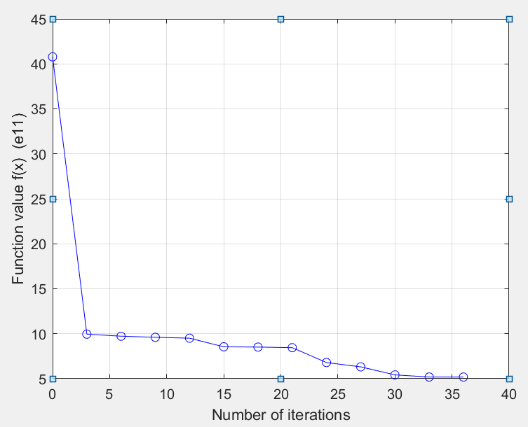
Figure 3. The objective function value of TTDSR method on Indian Pines dataset.

Theoretically, the SRI tensor is a low rank tensor. However, in the numerical experiments, we have no prior knowledge of the triple rank of the SRI tensor and the rank is given artificially. For the Indian Pines dataset, we run TTDSR algorithm ten times with the triple rank changing from 1 to 10 accordingly. In Fig.4, we demonstrate the values of R-SNR corresponding to different triple ranks. In this example, the best R-SNR is attained when the triple rank is 1.

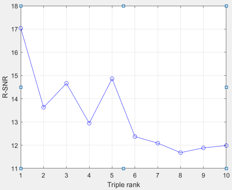
Figure 4. The R-SNR metric by TTDSR method on Indian Pines dataset for different triple rank.

7. Conclusion

In this work, we provide a novel tensor triple decomposition model for hyperspectral super-resolution. Firstly, in order to capture the global interdependence between hyperspectral data of different modes, we use triple rank to characterize its low rank. Then we propose a optimization algorithm TTDSR to get the desired hyperspectral super-resolution image. Using the triple decomposition theorem, we cleverly obtain the gradient of the objective function of the model, which provides great help for solving the problem. Due to the algebraic nature of the objective function $f(\mathbf{x})$, we apply the Kurdyka-$\L$ojasiewicz property in analyzing the convergence of the sequence of iterates generated by TTDSR. In addition, experiments on two published HSI datasets show the feasibility and effectiveness of the TTDSR. This work opens up a new prospect for realizing hyperspectral super-resolution by using various tensor decomposition.

Appendix A The process of vectorization of the variable

The gradient of the objective function in (12) is calculated by vectorization of the variable as

$$\mathbf{x}:=\left(\begin{array}[]{l}\mathbf{a}_{m_{1}rr}\\ \mathbf{b}_{m_{2}rr}\\ \mathbf{c}_{n_{3}rr}\end{array}\right)=\left(\begin{array}[]{c}A_{m_{1}rr\times 1}\\ B_{m_{2}rr\times 1}\\ C_{n_{3}rr\times 1}\end{array}\right).$$ (62)

We directly vectorize the optimal variables of (12) in accordance with preset principles while dealing with small-scale data. Firstly, noting that $f\left(\mathbf{x}\right)=f_{1}\left(\mathbf{x}\right)+f_{2}\left(\mathbf{x}\right)+f_{3}\left(\mathbf{x}\right).$ Secondly, vectorizing the known tensors $\mathcal{Y}_{h}$, $\mathcal{Y}_{m}$, we get

$$vec(\mathcal{Y}_{h})=\mathbf{d}_{h}\quad\quad and\quad\quad vec(\mathcal{Y}_{m})=\mathbf{d}_{m}.$$

The symbol $vec$ indicates the vectorization operator. It yields from (21) that

$${\left(\mathbf{y}_{h}\right)}_{n_{1}n_{2}n_{3}} =\left(\left(\left(C_{lm\times n_{3}}\otimes E_{n_{2}}\right)^{\top}\otimes P_{n_{1}\times{m_{1}}}\right)\left(\left(E_{m}\otimes K_{n\times n_{2}l}\right)^{\top}\otimes E_{m_{1}}\right)\right)\mathbf{a}_{m_{1}nm}$$

$$=\left(C_{n_{3}\times lm}\otimes E_{n_{2}}\otimes P_{n_{1}\times m_{1}}\right)\left(E_{m}\otimes K_{n_{2}l\times n}\otimes E_{m_{1}}\right)\mathbf{a}_{m_{1}nm}$$

$$=\left(C_{n_{3}\times lm}\otimes P_{n_{1}n_{2}\times m_{1}n_{2}}\right)\left(E_{m}\otimes K_{n_{2}l\times n}\otimes E_{m_{1}}\right)\mathbf{a}_{m_{1}nm}.$$

Hence,

$$f_{1}\left(\mathbf{x}\right)=\left\|\left(C_{n_{3}\times lm}\otimes P_{n_{1}n_{2}\times m_{1}n_{2}}\right)\left(E_{m}\otimes K_{n_{2}l\times n}\otimes E_{m_{1}}\right)\mathbf{a}_{m_{1}nm}-\mathbf{d}_{h}\right\|_{2}^{2}.$$

It is easy to see

$$\frac{\partial f_{1}(\mathbf{x})}{\partial\mathbf{a}_{m_{1}nm}}=2 \left(\left(C_{n_{3}\times lm}\otimes P_{n_{1}n_{2}\times m_{1}n_{2}}\right)\left(E_{m}\otimes K_{n_{2}l\times n}\otimes E_{m_{1}}\right)\right)^{\top}$$

$$\cdot\left(\left(C_{n_{3}\times lm}\otimes P_{n_{1}n_{2}\times m_{1}n_{2}}\right)\left(E_{m}\otimes K_{n_{2}l\times n}\otimes E_{m_{1}}\right)\mathbf{a}_{m_{1}nm}-\mathbf{d}_{h}\right)$$

$$= 2\left(E_{m}\otimes K_{n\times n_{2}l}\otimes E_{m_{1}}\right)\left(C_{lm\times n_{3}}\otimes P_{m_{1}n_{2}\times n_{1}n_{2}}\right)$$

$$\cdot\left(\left(C_{n_{3}\times lm}\otimes P_{n_{1}n_{2}\times m_{1}n_{2}}\right)\left(E_{m}\otimes K_{n_{2}l\times n}\otimes E_{m_{1}}\right)\mathbf{a}_{m_{1}nm}-\mathbf{d}_{h}\right).$$

Similarly, it yields from (24) that

$${\left(\mathbf{y}_{m}\right)}_{m_{1}m_{2}m_{3}} =\left(\left(\left(E_{m}\otimes B_{n\times m_{2}l}\right)\left(G_{lm\times m_{3}}\otimes E_{m_{2}}\right)\right)^{\top}\otimes E_{m_{1}}\right)\mathbf{a}_{m_{1}nm}$$

$$=\left(\left(G_{m_{3}\times lm}\otimes E_{m_{1}m_{2}}\right)\left(E_{m}\otimes B_{m_{2}l\times n}\otimes E_{m_{1}}\right)\right)\mathbf{a}_{m_{1}nm}.$$

Hence,

$$f_{2}\left(\mathbf{x}\right)=\left\|\left(\left(G_{m_{3}\times lm}\otimes E_{m_{1}m_{2}}\right)\left(E_{m}\otimes B_{m_{2}l\times n}\otimes E_{m_{1}}\right)\right)\mathbf{a}_{m_{1}nm}-\mathbf{d}_{m}\right\|_{2}^{2},$$

and

$$\frac{\partial f_{2}(\mathbf{x})}{\partial\mathbf{a}_{m_{1}nm}}=2 \left(\left(G_{m_{3}\times lm}\otimes E_{m_{1}m_{2}}\right)\left(E_{m}\otimes B_{m_{2}l\times n}\otimes E_{m_{1}}\right)\right)^{\top}$$

$$\cdot\left(\left(G_{m_{3}\times lm}\otimes E_{m_{1}m_{2}}\right)\left(E_{m}\otimes B_{m_{2}l\times n}\otimes E_{m_{1}}\right)\mathbf{a}_{m_{1}nm}-\mathbf{d}_{m}\right)$$

$$=2 \left(E_{m}\otimes B_{n\times m_{2}l}\otimes E_{m_{1}}\right)\left(G_{lm\times m_{3}}\otimes E_{m_{1}m_{2}}\right)$$

$$\cdot\left(\left(G_{m_{3}\times lm}\otimes E_{m_{1}m_{2}}\right)\left(E_{m}\otimes B_{m_{2}l\times n}\otimes E_{m_{1}}\right)\mathbf{a}_{m_{1}nm}-\mathbf{d}_{m}\right).$$

For $f_{3}\left(\mathbf{x}\right)=\mu\left\|\mathbf{x}\right\|_{2}^{2}$, we have

$$\frac{\partial f_{3}(\mathbf{x})}{\partial\mathbf{a}_{m_{1}nm}}=2\mu\mathbf{a}_{m_{1}nm}.$$

In a word,

$$\begin{split}\frac{\partial f(\mathbf{x})}{\partial\mathbf{a}_{m_{1}nm}}&=2\left(E_{m}\otimes K_{n\times n_{2}l}\otimes E_{m_{1}}\right)\left(C_{lm\times n_{3}}\otimes P_{m_{1}n_{2}\times n_{1}n_{2}}\right)\\ &\cdot\left(\left(\left(C_{n_{3}\times lm}\otimes P_{n_{1}n_{2}\times m_{1}n_{2}}\right)\left(E_{m}\otimes K_{n_{2}l\times n}\otimes E_{m_{1}}\right)\right)\mathbf{a}_{m_{1}nm}-\mathbf{d}_{h}\right)\\ &+2\left(E_{m}\otimes B_{n\times m_{2}l}\otimes E_{m_{1}}\right)\left(G_{lm\times m_{3}}\otimes E_{m_{1}m_{2}}\right)\\ &\cdot\left(\left(\left(G_{m_{3}\times lm}\otimes E_{m_{1}m_{2}}\right)\left(E_{m}\otimes B_{m_{2}l\times n}\otimes E_{m_{1}}\right)\right)\mathbf{a}_{m_{1}nm}-\mathbf{d}_{m}\right)\\ &+2\mu\mathbf{a}_{m_{1}nm}.\end{split}$$ (63)

It yields from (22) and (25) that

$$f_{1}\left(\mathbf{x}\right)=\left\|\left(\left(H_{n_{1}\times mn}\otimes P_{n_{2}n_{3}\times m_{2}n_{3}}\right)\left(E_{n}\otimes C_{n_{3}m\times l}\otimes E_{m_{2}}\right)\right)\mathbf{b}_{m_{2}ln}-\mathbf{d}_{h}\right\|_{2}^{2},$$

$$f_{2}\left(\mathbf{x}\right)=\left\|\left(\left(A_{m_{1}\times mn}\otimes E_{m_{2}m_{3}}\right)\left(E_{n}\otimes G_{m_{3}m\times l}\otimes E_{m_{2}}\right)\right)\mathbf{b}_{m_{2}ln}-\mathbf{d}_{m}\right\|_{2}^{2},$$

and

$$f_{3}\left(\mathbf{x}\right)=\mu\left\|\mathbf{x}\right\|_{2}^{2}.$$

Therefore,

$$\frac{\partial f(\mathbf{x})}{\partial\mathbf{b}_{m_{2}ln}} =2\left(E_{n}\otimes C_{l\times n_{3}m}\otimes E_{m_{2}}\right)\left(H_{mn\times n_{1}}\otimes P_{m_{2}n_{3}\times n_{2}n_{3}}\right)$$ (64)

$$\cdot\left(\left(\left(H_{n_{1}\times mn}\otimes P_{n_{2}n_{3}\times m_{2}n_{3}}\right)\left(E_{n}\otimes C_{n_{3}m\times l}\otimes E_{m_{2}}\right)\right)\mathbf{b}_{m_{2}LN}-\mathbf{d}_{h}\right)$$

$$+2\left(E_{n}\otimes G_{l\times m_{3}m}\otimes E_{m_{2}}\right)\left(A_{mn\times m_{1}}\otimes E_{m_{2}m_{3}}\right)$$

$$\cdot\left(\left(\left(A_{m_{1}\times mn}\otimes E_{m_{2}m_{3}}\right)\left(E_{n}\otimes G_{m_{3}m\times l}\otimes E_{m_{2}}\right)\right)\mathbf{b}_{m_{2}ln}-\mathbf{d}_{m}\right)$$

$$+2\mu\mathbf{b}_{m_{2}ln}.$$

It also yields from (23) and (26) that

$$f_{1}\left(\mathbf{x}\right)=\left\|\left(\left(H_{n_{1}\times nm}\otimes E_{n_{2}n_{3}}\right)\left(E_{m}\otimes K_{n_{2}n\times l}\otimes E_{n_{3}}\right)\right)\mathbf{c}_{n_{3}lm}-\mathbf{d}_{h}\right\|_{2}^{2},$$

$$f_{2}\left(\mathbf{x}\right)=\left\|\left(\left(A_{m_{1}\times nm}\otimes P_{{m_{2}m_{3}}\times m_{2}n_{3}}\right)\left(E_{m}\otimes B_{m_{2}n\times l}\otimes E_{n_{3}}\right)\right)\mathbf{c}_{n_{3}lm}-\mathbf{d}_{m}\right\|_{2}^{2},$$

and

$$f_{3}\left(\mathbf{x}\right)=\mu\left\|\mathbf{x}\right\|_{2}^{2}.$$

Thus,

$$\begin{split}\frac{\partial f(\mathbf{x})}{\partial\mathbf{c}_{n_{3}lm}}&=2\left(E_{m}\otimes K_{l\times n_{2}n}\otimes E_{n_{3}}\right)\left(H_{nm\times n_{1}}\otimes E_{n_{2}\times n_{3}}\right)\\ &\cdot\left(\left(\left(H_{n_{1}\times nm}\otimes E_{n_{2}\times n_{3}}\right)\left(E_{m}\otimes K_{n_{2}n\times l}\otimes E_{n_{3}}\right)\right)\mathbf{c}_{n_{3}lm}-\mathbf{d}_{h}\right)\\ &+2\left(E_{m}\otimes B_{l\times m_{2}n}\otimes E_{n_{3}}\right)\left(A_{nm\times m_{1}}\otimes P_{m_{2}n_{3}\times m_{2}m_{3}}\right)\\ &\cdot\left(\left(\left(A_{m_{1}\times nm}\otimes P_{m_{2}m_{3}\times m_{2}n_{3}}\right)\left(E_{m}\otimes B_{m_{2}n\times l}\otimes E_{n_{3}}\right)\right)\mathbf{c}_{n_{3}lm}-\mathbf{d}_{m}\right)\\ &+2\mu\mathbf{c}_{n_{3}lm}.\end{split}$$ (65)

Then, its gradient is

$$\nabla f(\mathbf{x})=2\left(\begin{split}&\left(E_{m}\otimes K_{n\times n_{2}l}\otimes E_{m_{1}}\right)\left(C_{lm\times n_{3}}\otimes P_{m_{1}n_{2}\times n_{1}n_{2}}\right)\\ &\cdot\left(\left(\left(C_{n_{3}\times lm}\otimes P_{n_{1}n_{2}\times m_{1}n_{2}}\right)\left(E_{m}\otimes K_{n_{2}l\times n}\otimes E_{m_{1}}\right)\right)\mathbf{a}_{m_{1}nm}-\mathbf{d}_{h}\right)\\ &+2\left(E_{m}\otimes B_{n\times m_{2}l}\otimes E_{m_{1}}\right)\left(G_{lm\times m_{3}}\otimes E_{m_{1}m_{2}}\right)\\ &\cdot\left(\left(\left(G_{m_{3}\times lm}\otimes E_{m_{1}m_{2}}\right)\left(E_{m}\otimes B_{m_{2}l\times n}\otimes E_{m_{1}}\right)\right)\mathbf{a}_{m_{1}nm}-\mathbf{d}_{m}\right)\\ &+2\mu\mathbf{a}_{m_{1}nm}\\ &\rule[-10.0pt]{256.0748pt}{0.50003pt}\\ &\left(E_{n}\otimes C_{l\times n_{3}m}\otimes E_{m_{2}}\right)\left(H_{mn\times n_{1}}\otimes P_{m_{2}n_{3}\times n_{2}n_{3}}\right)\\ &\cdot\left(\left(\left(H_{n_{1}\times mn}\otimes P_{n_{2}n_{3}\times m_{2}n_{3}}\right)\left(E_{n}\otimes C_{n_{3}m\times l}\otimes E_{m_{2}}\right)\right)\mathbf{b}_{m_{2}ln}-\mathbf{d}_{h}\right)\\ &+2\left(E_{n}\otimes G_{l\times m_{3}m}\otimes E_{m_{2}}\right)\left(A_{mn\times m_{1}}\otimes E_{m_{2}m_{3}}\right)\\ &\cdot\left(\left(\left(A_{m_{1}\times mn}\otimes E_{m_{2}m_{3}}\right)\left(E_{n}\otimes G_{m_{3}m\times l}\otimes E_{m_{2}}\right)\right)\mathbf{b}_{m_{2}ln}-\mathbf{d}_{m}\right)\\ &+2\mu\mathbf{b}_{m_{2}ln}\\ &\rule[-10.0pt]{256.0748pt}{0.50003pt}\\ &\left(E_{m}\otimes K_{l\times n_{2}n}\otimes E_{n_{3}}\right)\left(H_{nm\times n_{1}}\otimes E_{n_{2}\times n_{3}}\right)\\ &\cdot\left(\left(\left(H_{n_{1}\times nm}\otimes E_{n_{2}\times n_{3}}\right)\left(E_{m}\otimes K_{n_{2}n\times l}\otimes E_{n_{3}}\right)\right)\mathbf{c}_{n_{3}lm}-\mathbf{d}_{h}\right)\\ &+2\left(E_{m}\otimes B_{l\times m_{2}n}\otimes E_{n_{3}}\right)\left(A_{nm\times m_{1}}\otimes P_{m_{2}n_{3}\times m_{2}m_{3}}\right)\\ &\cdot\left(\left(\left(A_{m_{1}\times nm}\otimes P_{m_{2}m_{3}\times m_{2}n_{3}}\right)\left(E_{m}\otimes B_{m_{2}n\times l}\otimes E_{n_{3}}\right)\right)\mathbf{c}_{n_{3}lm}-\mathbf{d}_{m}\right)\\ &+2\mu\mathbf{c}_{n_{3}lm}\end{split}\right).$$ (66)

Appendix B We introduce five lemmas for the proof of Lemma 5.2

First, we consider the BFGS update $(\ref{4.1}),(\ref{4.2}),(\ref{4.3})$.

Lemma B.1.

Suppose that $H_{k+1}$ is generated by $(\ref{4.3})$. Then, we have

$$\left\|H_{k+1}\right\|\leq\left\|H_{k}\right\|\left(1+\frac{2MN}{\epsilon}\right)^{2}+\frac{N^{2}}{\epsilon}.$$ (67)

Proof.

If $\mathbf{y}_{k}^{\top}\mathbf{s}_{k}<{\epsilon}$, we get $\rho_{k}=0$ and $H_{k+1}=H_{k}$. Hence, the inequality (67) holds. Next, we consider the case $\mathbf{y}_{k}^{\top}\mathbf{s}_{k}\geq\epsilon$. Obviously, $\rho_{k}\leq\frac{1}{\epsilon}$. From Lemma 5.1 and $\left\{\mathbf{x}_{k}\right\}$ is bouned, suppose there exists a positive number $N$ such that $\left\|\mathbf{s}_{k}\right\|\leq N$ and we get

$$\left\|\mathbf{y}_{k}\right\|\leq 2M.$$ (68)

Since

$$\left\|V_{k}\right\|\leq 1+\rho_{k}\left\|\mathbf{y}_{k}\right\|\left\|\mathbf{s}_{k}\right\|\leq 1+\frac{2MN}{\epsilon}\quad\text{ and }\quad\left\|\rho_{k}\mathbf{s}_{k}\mathbf{s}_{k}^{\top}\right\|\leq\rho_{k}\left\|\mathbf{s}_{k}\right\|^{2}\leq\frac{N^{2}}{\epsilon},$$ (69)

we have

$$\left\|H_{k+1}\right\|\leq\left\|H_{k}\right\|\left\|V_{k}\right\|^{2}+\left\|\rho_{k}\mathbf{s}_{k}\mathbf{s}_{k}^{\top}\right\|\leq\left\|H_{k}\right\|\left(1+\frac{2MN}{\epsilon}\right)^{2}+\frac{N^{2}}{\epsilon}.$$ (70)

Hence, the inequality (67) is valid. ∎

Lemma B.2.

Suppose that $H_{k}$ is positive definite and $H_{k+1}$ is generated by BFGS $(\ref{4.1}),(\ref{4.2}),(\ref{4.3})$. Let $\lambda_{\min}(H)$ be the smallest eigenvalue of a symmetric matrix $H$. Then, we get $H_{k+1}$ is positive definite and

$$\lambda_{\min}\left(H_{k+1}\right)\geq\frac{\epsilon}{\epsilon+4M^{2}\left\|H_{k}\right\|}\lambda_{\min}\left(H_{k}\right).$$ (71)

Proof.

For any unit vector $\mathbf{v}$, we have

$$\mathbf{v}^{\top}H_{k+1}\mathbf{v}=\left(\mathbf{v}-\rho_{k}\mathbf{s}_{k}^{\top}\mathbf{vy}_{k}\right)^{\top}H_{k}\left(\mathbf{v}-\rho_{k}\mathbf{s}_{k}^{\top}\mathbf{vy}_{k}\right)+\rho_{k}\left(\mathbf{s}_{k}^{\top}\mathbf{v}\right)^{2}.$$ (72)

Let $t\equiv\mathbf{s}_{k}^{\top}\mathbf{v}$ and

$$\phi(t)\equiv\left(\mathbf{v}-t\rho_{k}\mathbf{y}_{k}\right)^{\top}H_{k}\left(\mathbf{v}-t\rho_{k}\mathbf{y}_{k}\right)+\rho_{k}t^{2}.$$ (73)

Because $H_{k}$ is positive definite, $\phi(t)$ is convex and attaches its minimum at $t_{*}=\frac{\rho_{k}\mathbf{y}_{k}^{\top}H_{k}\mathbf{v}}{\rho_{k}+\rho_{k}^{2}\mathbf{y}_{k}^{\top}H_{k}\mathbf{y}_{k}}$ . Hence,

$$\mathbf{v}^{\top}H_{k+1}\mathbf{v} \geq\phi\left(t_{*}\right)$$ (74)

$$=\mathbf{v}^{\top}H_{k}\mathbf{v}-t_{*}\rho_{k}\mathbf{y}_{k}^{\top}H_{k}\mathbf{v}$$

$$=\frac{\rho_{k}\mathbf{v}^{\top}H_{k}\mathbf{v}+\rho_{k}^{2}\left(\mathbf{y}_{k}^{\top}H_{k}\mathbf{y}_{k}\mathbf{v}^{\top}H_{k}\mathbf{v}-\left(\mathbf{y}_{k}^{\top}H_{k}\mathbf{v}\right)^{2}\right)}{\rho_{k}+\rho_{k}^{2}\mathbf{y}_{k}^{\top}H_{k}\mathbf{y}_{k}}$$

$$\geq\frac{\mathbf{v}^{\top}H_{k}\mathbf{v}}{1+\rho_{k}\mathbf{y}_{k}^{\top}H_{k}\mathbf{y}_{k}}>0,$$

where the penultimate inequality holds because the Cauchy-Schwarz inequality is valid for the positive definite matrix norm $\|\cdot\|_{H_{k}}$,

$$\left\|\mathbf{y}_{k}\right\|_{H_{k}}\|\mathbf{v}\|_{H_{k}}\geq\mathbf{y}_{k}^{\top}H_{k}\mathbf{v}.$$ (75)

So $H_{k+1}$ is also positive definite. From (68), it is easy to verify that

$$1+\rho_{k}\mathbf{y}_{k}^{\top}H_{k}\mathbf{y}_{k}\leq 1+\frac{4M^{2}\left\|H_{k}\right\|}{\epsilon}.$$ (76)

Thus, we have

$$\mathbf{v}^{\top}H_{k+1}\mathbf{v}\geq\frac{\epsilon}{{\epsilon}+4M^{2}\left\|H_{k}\right\|}\lambda_{\min}\left(H_{k}\right).$$ (77)

Hence, we get the validation of (71). ∎

Second, we turn to L-BFGS. Regardless of the selection of $\gamma_{k}$ in (19), we get the following lemma.

Lemma B.3.

Suppose that the parameter $\gamma_{k}$ takes Barzilai-Borwein steps $(\ref{4.6})$ . Then, we have

$$\frac{\epsilon}{4M^{2}}\leq\gamma_{k}\leq\frac{N^{2}}{\epsilon}.$$ (78)

Proof.

If $\mathbf{y}_{k}^{\top}\mathbf{s}_{k}<\epsilon$, we get $\gamma_{k}=1$ which satisfies the bounds in (78) obviously. Otherwise, we have

$$\epsilon\leq\mathbf{y}_{k}^{\top}\mathbf{s}_{k}\leq\left\|\mathbf{y}_{k}\right\|\left\|\mathbf{s}_{k}\right\|.$$ (79)

Recalling (68), we get

$$\frac{\epsilon}{N}\leq\left\|\mathbf{y}_{k}\right\|\leq 2M\quad\text{ and }\quad\frac{\epsilon}{2M}\leq\left\|\mathbf{s}_{k}\right\|\leq N.$$ (80)

Hence, we have

$$\frac{\epsilon}{4M^{2}}\leq\frac{\mathbf{y}_{k}^{\top}\mathbf{s}_{k}}{\left\|\mathbf{y}_{k}\right\|^{2}}\leq\frac{\left\|\mathbf{y}_{k}\right\|\left\|\mathbf{s}_{k}\right\|}{\left\|\mathbf{y}_{k}\right\|^{2}}=\frac{\left\|\mathbf{s}_{k}\right\|}{\left\|\mathbf{y}_{k}\right\|}=\frac{\left\|\mathbf{s}_{k}\right\|^{2}}{\left\|\mathbf{y}_{k}\right\|\left\|\mathbf{s}_{k}\right\|}\leq\frac{\left\|\mathbf{s}_{k}\right\|^{2}}{\mathbf{y}_{k}^{\top}\mathbf{s}_{k}}\leq\frac{N^{2}}{\epsilon}.$$ (81)

which means that $\gamma_{k}^{\mathrm{BB}1}$ and $\gamma_{k}^{\mathrm{BB}2}$ satisfy (78). ∎

Third, based on Lemmas B.1, B.2, B.3, we obtain two lemmas as follows.

Lemma B.4.

Suppose that the approximation of a Hessian’s inverse $H_{k}$ is generated by L-BFGS $(\ref{4.4}),(\ref{4.5})$. Then, there exists a positive constant $C_{M}\geq 1$ such that

$$\left\|H_{k}\right\|\leq C_{M}.$$ (82)

Proof.

From Lemma B.3 and (18), we have $\left\|H_{k}^{(0)}\right\|\leq\frac{N^{2}}{\epsilon}$. Then, for (17) and Lemma B.1, we get

$$\left\|H_{k}\right\| \leq\left\|H_{k-1}\right\|\left(1+\frac{2MN}{\epsilon}\right)^{2}+\frac{N^{2}}{\epsilon}$$ (83)

$$\leq\cdots$$

$$\leq\left\|H_{k}^{(0)}\right\|\left(1+\frac{2MN}{\epsilon}\right)^{2l}+\frac{N^{2}}{\epsilon}\sum_{m=1}^{l-1}\left(1+\frac{2MN}{\epsilon}\right)^{2m}$$

$$\leq\frac{N^{2}}{\epsilon}\sum_{m=1}^{l}\left(1+\frac{2MN}{\epsilon}\right)^{2m}\equiv C_{M}.$$

Thus (82) holds. ∎

Lemma B.5.

Suppose that the approximation of a Hessian’s inverse $H_{k}$ is generated by L-BFGS $(\ref{4.4}),(\ref{4.5})$. Then, there exists a constant $0<C_{m}<1$ such that

$$\lambda_{\min}\left(H_{k}\right)\geq C_{m}.$$ (84)

Proof.

From Lemma B.3 and (18), we have $\lambda_{\min}\left(H_{k}^{(0)}\right)\geq\frac{\epsilon}{4M^{2}}.$ Moreover, Lemma B.4 means $\left\|H_{k-m}\right\|\leq C_{M}$ for all $m=1,\ldots,l$. Hence, Lemma B.2 implies

$$\lambda_{\min}\left(H_{k-m+1}\right)\geq\frac{\epsilon}{{\epsilon}+4M^{2}C_{M}}\lambda_{\min}\left(H_{k-m}\right).$$ (85)

Then, we obtain

$$\lambda_{\min}\left(H_{k}\right) \geq\frac{\epsilon}{{\epsilon}+4M^{2}C_{M}}\lambda_{\min}\left(H_{k-1}\right)$$ (86)

$$\geq\cdots$$

$$\geq\left(\frac{\epsilon}{{\epsilon}+4M^{2}C_{M}}\right)^{l}\lambda_{\min}\left(H_{k}^{(0)}\right)$$

$$\geq\frac{\epsilon}{4M^{2}}\left(\frac{\epsilon}{{\epsilon}+4M^{2}C_{M}}\right)^{l}\equiv C_{m}.$$

Finally, the proof of Lemma 5.2 is straightforward from Lemmas B.4 and B.5. ∎

Use of AI tools declaration

The article does not use Artificial Intelligence (AI) tools.

Received xxxx 20xx; revised xxxx 20xx; early access xxxx 20xx.

References

- [1] B. Aiazzi, S. Baronti and M. Selva, \doititleImproving component substitution pansharpening through multivariate regression of MS +Pan data, IEEE Trans. Geosci. Remote Sens., 45 (2007), 3230-3239. 10.1109/tgrs.2007.901007
- [2] H. Attouch, J. Bolte, P. Redont and A. Soubeyran, \doititleProximal alternating minimization and projection methods for nonconvex problems: An approach based on the Kurdyka-ojasiewicz inequality, Math. Oper. Res., 35 (2010), 438-457.
- [3] J. Barzilai and J. M. Borwein, \doititleTwo-point step size gradient methods, IMA. J. Numer. Anal, 8 (1988), 141-148.
- [4] J. M. Bioucas-Dias, A. Plaza, G. Camps-Valls, P. Scheunders, N. Nasrabadi and J. Chanussot, \doititleHyperspectral remote sensing data analysis and future challenges, IEEE Geosci. Remote Sens. Mag., 1 (2013), 6-36.
- [5] R. A. Borsoi, C. Prvost, K. Usevich, D. Brie, J. C. Bermudez, and C. Richard, \doititleCoupled tensor decomposition for hyperspectral and multispectral image fusion with inter-image variability, IIEEE J. Sel. Top. Signal Process., 15 (2021),702-717.
- [6] P. Chavez, S. C. Sides and J. A. Anderson, \doititleComparison of three different methods to merge multiresolution and multispectral data-Landsat TM and SPOT panchromatic, Photogramm. Eng. Remote Sens., 57 (1991), 295-303.
- [7] C. I. Chang and S.S. Chiang, \doititle Anomaly detection and classification for hyperspectral imagery, IEEE Trans. Geosci. Remote Sens., 40 (2002), 1314-1325.
- [8] G. Camps-Valls and L. Bruzzone, \doititle Kernel-based methods for hyperspectral image classification, IEEE Trans. Geosci. Remote Sens., 43 (2005), 1351-1362.
- [9] Z. Chen, H. Pu, B. Wang and G. M. Jiang, \doititleFusion of hyperspectral and multispectral images: A novel framework based on generalization of pan-sharpening methods, IEEE Geosci. Remote Sens. Lett., 11 (2014), 1418-1422.
- [10] J. Chang J, Y. Chen, L. Qi, \doititleComputing eigenvalues of large scale sparse tensors arising from a hypergraph, SIAM J. Sci. Comput., 38 (2016), A3618-A3643.
- [11] Y. Chen, X. Zhang, L. Qi and Y. Xu, \doititleA Barzilai Borwein gradient algorithm for spatio-temporal internet traffic data completion via tensor triple decomposition, SIAM J. Sci. Comput., 88 (2021), 1-24.
- [12] E. J. Cands, X. Li, Y. Ma and J. Wright, \doititleRobust principal component analysis?, J. ACM, 58 (2011), 1-37.
- [13] R. Dian and S. Li, \doititleHyperspectral image super-resolution via subspace-based low tensor multi-rank regularization, IEEE Trans. Image Process., 28 (2019), 5135-5146.
- [14] GIC, Grupo de inteligencia computacional, 2014. Available from: http://www.ehu.eus/ccwintco/index.php?title=HyperspectralRemoteSensingScenes.
- [15] R. C. Hardie, M. T. Eismann and G. L. Wilson, \doititleMAP estimation for hyperspectral image resolution enhancement using an auxiliary sensor, IEEE Trans. Image Process., 13 ( 2004), 1174-1184.
- [16] W. He, Y. Chen, N. Yokoya, C. Li and Q. Zhao, \doititleHyperspectral super-resolution via coupled tensor ring factorization, Pattern Recognit., 122 (2022), 108280.
- [17] T. Imbiriba, R. A. Borsoi, J. C. M. Bermudez, \doititleLow-rank tensor modeling for hyperspectral unmixing accounting for spectral variability, IEEE Trans. Geosci. Remote Sens., 58 (2019), 1833-1842.
- [18] N. Keshava, J. F. Mustard, \doititleSpectral unmixing, IEEE Signal Process. Mag., 19 (2002), 44-57.
- [19] R. Kawakami, Y. Matsushita, J. Wright, M. Ben-Ezra, Y. W. Tai, and K. Ikeuchi, \doititleHigh-resolution hyperspectral imaging via matrix factorization, Conference on Computer Vision and Pattern Recognition(CVPR), IEEE, (2011), 2329-2336.
- [20] C. I. Kanatsoulis, X. Fu, N. D. Sidiropoulos and W. K. Ma, \doititleHyperspectral super-resolution: A coupled tensor factorization approach, IEEE Trans. Signal Process., 66 (2018), 6503-6517.
- [21] D. C. Liu and J. Nocedal, \doititleOn the limited memory BFGS method for large scale optimization, Math. Program., 45 (1989), 503-528.
- [22] J. G. Liu, \doititleSmoothing filter-based intensity modulation: A spectral preserve image fusion technique for improving spatial details, Int. J. Remote Sens., 21 (2000), 3461-3472.
- [23] X. Liu, S. Bourennane, C. Fossati, \doititleDenoising of hyperspectral images using the PARAFAC model and statistical performance analysis, IEEE Trans. Geosci. Remote Sens., 50 ( 2012), 3717-3724.
- [24] S. Li, R. Dian, L. Fang and J. M. Bioucas-Dias, \doititleFusing hyperspectral and multispectral images via coupled sparse tensor factorization, IEEE Trans. Image Process., 27 (2018), 4118-4130.
- [25] D. Manolakis and G. Shaw, \doititleDetection algorithms for hyperspectral imaging applications, IEEE Signal Process. Mag., 19 (2002), 29-43.
- [26] N. Vervliet, O. Debals, L. Sorber, M. Van Barel and L. De Lathauwer, \doititleTensorlab 3.0, 2016. Available from: http://www.tensorlab.net.
- [27] X. Otazu, M. Gonzlez-Audcana and O. Fors, \doititleIntroduction of sensor spectral response into image fusion methods. Application to wavelet-based methods, IEEE Trans. Geosci. Remote Sens., 43 (2005), 2376-2385.
- [28] C. Prvost, K. Usevich, P. Comon and D. Brie, \doititleHyperspectral super-resolution with coupled tucker approximation: Recoverability and SVD-based algorithms, IEEE Trans. Signal Process., 68 (2020), 931-946.
- [29] L. Qi, Y. Chen, M. Bakshi and X. Zhang, \doititleTriple decomposition and tensor recovery of third order tensors. SIAM Journal on Matrix Analysis and Applications, IEEE Trans. Signal Process., 42 (2021), 299-329.
- [30] M. Selva, B. Aiazzi, F. Butera, L. Chiarantini and S. Baronti, \doititleHyper-sharpening: A first approach on SIM-GA data, IEEE J. Sel. Top. Appl. Earth Observ. Remote Sens., 8 (2015), 3008-3024.
- [31] M. Simoes, J. Bioucas-Dias, L. B. Almeida and J. Chanussot, \doititleA convex formulation for hyperspectral image superresolution via subspace-based regularization, IEEE Trans. Geosci. Remote Sens., 53 (2014), 3373-3388.
- [32] G. Vivone, L. Alparone, J. Chanussot, M. Dalla Mura, A. Garzelli, G. A. Licciardi and L. Wald, \doititleA critical comparison among pansharpening algorithms, IEEE Trans. Geosci. Remote Sens., 53 (2014), 2565-2586.
- [33] M. A. Veganzones, J. E. Cohen, R. C. Farias, J. Chanussot and P. Comon, \doititleNonnegative tensor CP decomposition of hyperspectral data, IEEE Trans. Geosci. Remote Sens., 54 (2015), 2577-2588.
- [34] Q. Wei, J. Bioucas-Dias, N. Dobigeon and J. Y. Tourneret, \doititleHyperspectral and multispectral image fusion based on a sparse representation, IEEE Trans. Geosci. Remote Sens., 53 (2015), 3658-3668.
- [35] Q. Wei, N. Dobigeon and J. Y. Tourneret, \doititleFast fusion of multi-band images based on solving a Sylvester equation, IEEE Trans. Image Process, 24 (2015), 4109-4121.
- [36] L. Wald, T. Ranchin and M. Mangolini, \doititleFusion of satellite images of different spatial resolutions: Assessing the quality of resulting images, Photogramm. Eng. Remote Sens., 63 (1997), 691-699.
- [37] Y. Xu, Z. Wu, J. Li, A. Plaza and Z. Wei, \doititleAnomaly detection in hyperspectral images based on low-rank and sparse representation, IEEE Trans. Geosci. Remote Sens, 54 (2015), 1990-2000.
- [38] X. Xu and Z. Shi, \doititleMulti-objective based spectral unmixing for hyperspectral images, ISPRS-J. Photogramm. Remote Sens., 124 (2017), 54-69.
- [39] T. Xu, T. Z. Huang, L. J. Deng, X. L. Zhao and J. Huang, \doititleHyperspectral image superresolution using unidirectional total variation with tucker decomposition, IEEE J. Sel. Top. Appl. Earth Observ. Remote Sens., 13 (2020), 4381-4398.
- [40] N. Yokoya, T. Yairi, A. Iwasaki, X. L. Zhao and J. Huang, \doititleCoupled nonnegative matrix factorization unmixing for hyperspectral and multispectral data fusion, IEEE Trans. Geosci. Remote Sens., 50 (2011), 528-537.
- [41] N. Yokoya, C. Grohnfeldt and J. Chanussot, \doititleHyperspectral and multispectral data fusion: A comparative review of the recent literature, IEEE Geosci. Remote Sens. Mag., 5 (2017), 29-56.
- [42] K. Zhang, M. Wang, S. Yang and L. Jiao, \doititleSpatial-spectral-graph-regularized low-rank tensor decomposition for multispectral and hyperspectral image fusion, IEEE J. Sel. Top. Appl. Earth Observ. Remote Sens., 11 (2018), 1030-1040.
- [43] K. Zhang, M. Wang, S. Yang, X. L. Zhao and J. Huang, \doititleMultispectral and hyperspectral image fusion based on group spectral embedding and low-rank factorization, IEEE Trans. Geosci. Remote Sens., 55 (2016), 1363-1371.
- [44] M. Zare, M. S. Helfroush, K. Kazemi and P. Scheunders, \doititleHyperspectral and multispectral image fusion using coupled non-negative tucker tensor decomposition, Remote Sens., 13 (2021), 2930.