Dynamical Analysis of the Dirac-Born-Infeld type of Tachyon field minimally coupled with barotropic fluid using EOS parametrization of a field

Abstract

In this paper, we present a dynamical system analysis of the tachyon dark energy model by parametrization of the equation of state (EoS) of the dark energy. The choice of parametrization can constrain the form of the field potential, and as a result, the theory can be directly constrained from the observation without assuming a particular form of the potential.

1 Introduction: the tachyon dynamics

The action of the field was first discovered in string theory[1, 2, 3] and later on it has been modeled to study the early time epoch as inflaton field[4, 5, 6, 7, 8] and a dark energy (DE) candidate in the late-time epoch[9, 10, 11, 12, 13, 14, 15, 16]. The action of the tachyon field is a Dirac-Born-Infeld (DBI) type and dark matter is characterized as pressureless perfect fluid; both are minimally coupled with gravity as follows:

$$S=\int_{\Omega}d^{4}x\sqrt{-g}\left[\frac{R}{2\kappa^{2}}-V(\phi)\sqrt{1+(\nabla_{\mu}\phi)(\nabla^{\mu}\phi)}\right]+S_{M}$$ (1)

where the first term in the action is the Einstein-Hilbert action, the second term corresponds to tachyon field, and the final term is the perfect fluid action. We conduct the analysis in the FLRW background metric $ds^{2}=-dt^{2}+a(t)^{2}d\vec{x}^{2}$, where $a$ is the scale factor; this is consistent with the observational fact that the universe appears flat, homogeneous, and isotropic at the largest scale. Due to the highly symmetric metric the field $\phi$ only depends on time. To analyze the dynamics of the action, it is necessary to obtain the equation of motion by varying the action with respect to the metric and field $(\delta g^{{\mu\nu}},\delta\phi)$. Variation of action with respect to metric yields Einstein field equation, i.e., $G_{{\mu\nu}}=\kappa^{2}(T_{{\mu\nu}}^{M}+T_{{\mu\nu}}^{\phi})$ and field equation of motion is $\ddot{\phi}+3H\dot{\phi}(1-\dot{\phi}^{2})+\frac{V_{,\phi}}{V}(1-\dot{\phi}^{2})=0.$ The energy density of the field is $\rho_{\phi}={V(\phi)}({1-\dot{\phi}^{2}})^{-1/2}$, and pressure is $P_{\phi}=-V(\phi)\ ({1-\dot{\phi}^{2}})^{1/2}$ and the field is to be depicted as dark energy it should exert negative pressure for which $V(\phi)>0$ and $\dot{\phi}^{2}\ll 1$. Typically, the acceleration is denoted by the EoS which is defined as the ratio of pressure to energy density. In the case of the tachyon field, the EoS is $\omega_{\phi}=-1+\dot{\phi}^{2}$. Since, the field is a dynamical quantity, its potential plays a crucial role in achieving late-time cosmic acceleration provided $\dot{\phi}^{2}\ll 1$. In this scenario, a broad class of potentials could be investigated, but doing so would not be an efficient task. Instead of choosing any specific potential we choose some approximate form of the EoS of the tachyon field. These equations are time dependent and parameterized phenomenologically. Such parameterized EoS of the DE can circumvent the selection of the potential, enabling the system to be constrained directly by the observation[17]. In this paper, we will evaluate the dynamics of the system using the parametrization $\omega_{\rm de}=\omega_{0}+\omega_{1}(t\dot{H}/H)$, [18]. To accomplish this, we will first define the minimal dimensionless dynamical variables required to transform the field equation of motions into three first order differential equation known as autonomous equations. The dimensionless variables are $x=\dot{\phi},\ y=\frac{\kappa\sqrt{V(\phi)}}{\sqrt{3}H},\ \lambda=-\frac{V_{,\phi}}{\kappa V^{\frac{3}{2}}},\ \Gamma=V\frac{V_{,\phi\phi}}{V_{,\phi}^{2}},\;\sigma^{2}=\frac{\kappa^{2}\rho_{M}}{3H^{2}}.$ The autonomous equations are $x^{\prime}=f(x,y,\lambda),y^{\prime}={h}(x,y,\lambda),\lambda^{\prime}=-\ \sqrt[]{3}\ \lambda^{2}xy\left(\Gamma-\frac{3}{2}\right)$. Therefore, to close the system, at least three variables are required, resulting in 3D phase space. $\Gamma$ depends on the choice of potential, in some instances, it can be constant or $\phi$ dependent. As, $\omega_{\rm de}$ equal to $\omega_{\phi}$, and by differentiating both side with respect to time, one obtains new $x^{\prime}=f_{1}(x,y,\lambda)$. Equating $f_{1}$ with $f$, $\lambda$ in $(x,y)$ can be determined. Using this $\lambda$ in the old $x^{\prime},y^{\prime}$, closes the system in only these two variables without requiring any additional variables, thereby reducing the phase space from 3D to 2D. Additionally, $\Gamma$ in $(x,y)$ can be obtained by taking the derivative of $\lambda$ and equating with its unconstrained $\lambda^{\prime}$. The dynamical equations in $(x^{\prime},y^{\prime})$ produce two stable critical points, $P_{2}$ and $P_{3}$ shown in the phase space $(x,y)$ in Fig.[2]. Point $P_{3}$ is independent of the model parameters and represents the de-Sitter phase of acceleration, whereas $P_{2}$ is a model parameter dependent $(\omega_{0},\omega_{1})$. The vector trajectories from the kinetic dominating region $\dot{\phi}^{2}\sim 1$, initially attract to the the matter phase point $P_{1}$, then to $P_{2}$. All field parameters vanish at point $P_{0}$, yielding a trivial non-accelerating fixed point. In Fig.[2], we solve the autonomous system from past to asymptotic future to discover observable parameter dynamics against $N$. In the past, the fluid density dominated field density and the effective EoS $\omega_{\rm tot}\sim 0$, identify as the matter phase. Field density dominates and the effective EoS approaches $-1$ as the system evolves, nevertheless the sound speed $c_{s}^{2}$ remain in causal limit.

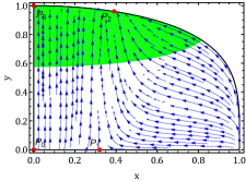
Figure 1: The phase space plot for $\omega_{0}=-0.9$ and $\omega_{1}=-0.05$, where green region shows the accelerating region $-1\leq\omega_{\rm tot}=-1-\frac{2\dot{H}}{3H^{2}}<-1/3$.

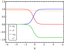
Figure 2: The evolution plot for $\omega_{0}=-0.9$ and $\omega_{1}=-0.05$ where field density $\Omega_{\phi}=y^{2}(1-x^{2})^{-1/2}$, fluid density $\sigma^{2}=1-\Omega_{\phi}$ and sound speed $0\leq c_{s}^{2}=\delta P_{\phi}/\delta\rho_{\phi}\leq 1$.

2 Conclusion

The given parametrization is compatible with the tachyon field and produces a stable accelerating fixed point. In the presence of pressureless background fluid, the field resembles the characteristics of dark energy. In addition, the method has been examined when both the dark sectors sector interacts $\nabla_{\mu}T^{{\mu\nu}}_{\phi}=-Q^{\nu};\nabla_{\mu}T^{{\mu\nu}}_{M}=Q^{\nu}$ and produces the stable accelerating solution see in ref.[17].

References

- [1] Ashoke Sen “Tachyon matter” In JHEP 07, 2002, pp. 065 DOI: 10.1088/1126-6708/2002/07/065
- [2] Ashoke Sen “Rolling tachyon” In JHEP 04, 2002, pp. 048 DOI: 10.1088/1126-6708/2002/04/048
- [3] Ashoke Sen “Field theory of tachyon matter” In Mod. Phys. Lett. A 17, 2002, pp. 1797–1804 DOI: 10.1142/S0217732302008071
- [4] Sergio Campo, Ramon Herrera and Adolfo Toloza “Tachyon Field in Intermediate Inflation” In Phys. Rev. D 79, 2009, pp. 083507 DOI: 10.1103/PhysRevD.79.083507
- [5] Ramon Herrera, Sergio Campo and C. Campuzano “Tachyon warm inflationary universe models” In JCAP 10, 2006, pp. 009 DOI: 10.1088/1475-7516/2006/10/009
- [6] A. Mohammadi, Kh Saaidi and T. Golanbari “Tachyon constant-roll inflation” In Phys. Rev. D 97.8, 2018, pp. 083006 DOI: 10.1103/PhysRevD.97.083006
- [7] J. Sadeghi and A. R. Amani “The Solution of tachyon inflation in curved universe” In Int. J. Theor. Phys. 48, 2009, pp. 14–21 DOI: 10.1007/s10773-008-9776-0
- [8] L. Raul W. Abramo and Fabio Finelli “Cosmological dynamics of the tachyon with an inverse power-law potential” In Phys. Lett. B 575, 2003, pp. 165–171 DOI: 10.1016/j.physletb.2003.09.065
- [9] Abolhassan Mohammadi et al. “Warm tachyon inflation and swampland criteria” In Chin. Phys. C 44.9, 2020, pp. 095101 DOI: 10.1088/1674-1137/44/9/095101
- [10] Gianluca Calcagni and Andrew R. Liddle “Tachyon dark energy models: dynamics and constraints” In Phys. Rev. D 74, 2006, pp. 043528 DOI: 10.1103/PhysRevD.74.043528
- [11] Ahmad Sheykhi “Holographic Scalar Fields Models of Dark Energy” In Phys. Rev. D 84, 2011, pp. 107302 DOI: 10.1103/PhysRevD.84.107302
- [12] Sudhakar Panda, M. Sami and Shinji Tsujikawa “Inflation and dark energy arising from geometrical tachyons” In Phys. Rev. D 73, 2006, pp. 023515 DOI: 10.1103/PhysRevD.73.023515
- [13] Ying Shao, Yuan-Xing Gui and Wei Wang “Parametrization of tachyon field” In Mod. Phys. Lett. A 22, 2007, pp. 1175–1182 DOI: 10.1142/S0217732307021809
- [14] Elsa M. Teixeira, Ana Nunes and Nelson J. Nunes “Conformally Coupled Tachyonic Dark Energy” In Phys. Rev. D 100.4, 2019, pp. 043539 DOI: 10.1103/PhysRevD.100.043539
- [15] P. P. Avelino, L. Losano and J. J. Rodrigues “Quintessence and tachyon dark energy models with a constant equation of state parameter” In Phys. Lett. B 699, 2011, pp. 10–14 DOI: 10.1016/j.physletb.2011.03.048
- [16] Edmund J. Copeland, Mohammad R. Garousi, M. Sami and Shinji Tsujikawa “What is needed of a tachyon if it is to be the dark energy?” In Phys. Rev. D 71, 2005, pp. 043003 DOI: 10.1103/PhysRevD.71.043003
- [17] Saddam Hussain, Saikat Chakraborty, Nandan Roy and Kaushik Bhattacharya “Dynamical systems analysis of tachyon-dark-energy models from a new perspective” In Phys. Rev. D 107.6, 2023, pp. 063515 DOI: 10.1103/PhysRevD.107.063515
- [18] A. A. Usmani et al. “The Dark energy equation of state” In Mon. Not. Roy. Astron. Soc. 386, 2008, pp. L92–95 DOI: 10.1111/j.1745-3933.2008.00468.x