Balanced Energy Regularization Loss
for Out-of-distribution Detection

Abstract

In the field of out-of-distribution (OOD) detection, a previous method that use auxiliary data as OOD data has shown promising performance. However, the method provides an equal loss to all auxiliary data to differentiate them from inliers. However, based on our observation, in various tasks, there is a general imbalance in the distribution of the auxiliary OOD data across classes. We propose a balanced energy regularization loss that is simple but generally effective for a variety of tasks. Our balanced energy regularization loss utilizes class-wise different prior probabilities for auxiliary data to address the class imbalance in OOD data. The main concept is to regularize auxiliary samples from majority classes, more heavily than those from minority classes. Our approach performs better for OOD detection in semantic segmentation, long-tailed image classification, and image classification than the prior energy regularization loss. Furthermore, our approach achieves state-of-the-art performance in two tasks: OOD detection in semantic segmentation and long-tailed image classification. Code is available at https://github.com/hyunjunChhoi/Balanced_Energy

1 Introduction

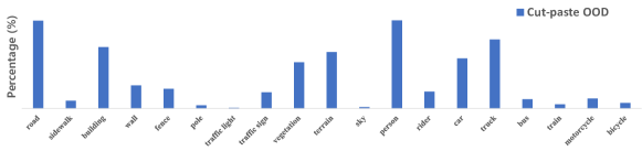
(a)

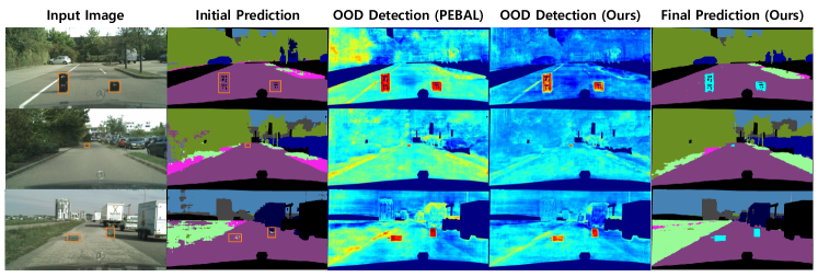
(b)

Figure 1: Overview of our approach in semantic segmentation task (a): Class distribution of cut-pasted OOD pixels collected from 10000 synthesized scene images ; (b): OOD detection result in Fishyscapes validation sets. Our balanced energy PEBAL(Ours) is the method that substitutes the energy regularization loss in PEBAL [41] with our balanced energy regularization loss.

Deep neural networks are used in a variety of fields such as image classification [22] and semantic segmentation [11]. However, there is a challenge in the practical use of deep neural networks in areas where safety is crucial, such as autonomous driving and medical diagnosis [20, 25]. In particular, deep neural networks have the issue of providing high confidence to out-of-distribution (OOD) samples that are not used for training [15]. As a result, Maximum softmax probability (MSP) score has been proposed to identify these OOD samples [17]. Based on the score, OOD detection performance is evaluated by metrics (e.g. AUROC, FPR). Both in image classification [26, 24, 40, 18, 29, 43, 46, 30, 38](including long-tailed image classification [43]) and semantic segmentation [16, 3, 1, 2, 28, 36, 33, 10, 19, 41, 12, 5], different approaches have been suggested to enhance the OOD detection performance. Among them, we concentrate on the methods using auxiliary data as OOD data which indicate superior OOD detection performance to the previous methods that only use in-distribution samples.

Outlier Exposure (OE) utilizes an auxiliary dataset of outliers to improve OOD detection performance [18]. The auxiliary data is consist of classes that do not overlap with the in-distribution data and the test OOD data. OE leverages the cross-entropy loss for the existing training data and the regularization loss for the auxiliary data. The cross-entropy loss that results from giving the auxiliary data a uniform label is the regularization loss of OE. Meanwhile, a new energy score has been introduced in Energy-based OOD detection (EnergyOE) which replaces the MSP score [29]. Furthermore, EnergyOE suggests an energy regularization loss that differs from that of OE to enhance performance. The squared hinge loss for energy with every existing (in-distribution) piece of data and every auxiliary (OOD) piece of data is added to create the energy regularization loss. Similarly, in semantic segmentation, the OOD detection performance is enhanced by using the auxiliary dataset of the outlier. Meta-OOD [5] organized the auxiliary dataset of the outlier by scenes of the COCO dataset [27]. Although the process of creating the auxiliary data is different from image classification, the training loss is comparable. Meta-OOD adopts the regularization loss proposed by OE. Recently, PEBAL [41] also adopts energy regularization loss proposed by EnergyOE.

However, when regularizing auxiliary data, the existing methods for OOD detection do not take into account variations between auxiliary data samples. The variations are severe especially on real data such as semantic segmentation for autonomous driving. As seen in Figure 1(a), for the pre-trained model, the class distribution of the auxiliary OOD data is not uniform across classes, i.e., imbalanced. To address the imbalanced problem, we regularize the auxiliary data differently for each sample. To achieve this, we propose a balanced energy regularization loss to apply higher regularization to majority classes than minority classes in auxiliary data. In other words, auxiliary samples of majority classes receive a larger energy constraint than samples of minority classes. We introduce the term $Z$, which indicates whether a sample belongs to the majority or minority of a class. $Z$ is the weighted sum of the softmax output of the classification model for a sample (i.e., the posterior probability of a class for a given sample), where the weight is the prior probability for the class. Unlike the existing energy regularization loss, our balanced energy regularization loss adjusts to the value of $Z$ for an auxiliary data sample. Two adaptive loss components make up our loss: loss margin and loss weight. The adaptive loss margin provides an additional $Z$-proportional margin in the squared hinge loss for auxiliary data. The adaptive loss weight gives a weight proportional to $Z$ to the squared hinge loss.

We confirm our novel loss in three tasks: semantic segmentation, long-tailed image classification, and image classification. The proposed loss is simple but generally effective for various tasks. Figure 1(b) illustrates how our method outperforms the previous state-of-the-art (SOTA) algorithm PEBAL in the semantic segmentation task by replacing the energy regularization loss with our loss. OOD detection performance is also enhanced when using our loss compared to the baseline (EnergyOE) which use only energy regularization loss. In all image classification tasks, we evaluate our method on semantically coherent OOD detection (SC-OOD) benchmark [46]. In long-tailed image classification task, our approach reveals superior OOD performance compared to both OE and EnergyOE methods which use auxiliary data. In addition, our approach outperforms the previous SOTA method PASCL [43], Similarly, in the image classification task, we demonstrate the superiority of our loss by outperforming both OE and EnergyOE, which make use of auxiliary data. The contributions are summarized as:

• By making inferences based on previously trained models, we explain the imbalanced distribution of auxiliary OOD data.

• We suggest a novel balanced energy regularization loss to address the class imbalance in auxiliary OOD data.

• The proposed balanced loss performs better for OOD detection than the previous energy regularization loss.

• The SOTA performance for OOD detection in two tasks is achieved by our OOD detection method.

2 Related Work

2.1 OOD in Image Classification

In the image classification task, there are two main approaches for OOD detection in deep neural networks. The first is a method to attain prediction uncertainty for a pre-trained model  [26, 40, 29, 24]. The second approach modifies the architecture or loss based on new training [18, 29, 15, 38, 9]. The first method primarily suggests new measures to boost performance. Proposed measures include the baseline MSP [17], Mahalanobis distance [24], the distance from the distribution of the Gram matrix [40], and free energy whose value is computed from the logit rather than the probability [29].

The second method mainly uses auxiliary data as OOD data to enhance performance. Representatively, there are OE [18] and EnergyOE [29] as methods of using auxiliary data for learning. OECC [38] replaced OE’s cross entropy loss with total variance loss and included calibration loss. In UDG [46], auxiliary data is once again divided into OOD samples and in-distribution samples through unsupervised dual grouping to improve performance. The more challenging SC-OOD benchmark is also proposed by UDG.

2.2 OOD in Semantic Segmentation

In general, semantic segmentation’s OOD detection benchmarks [3, 28, 16] resolve the detection problem of OOD that appears in complex urban driving scenes [8]. The assessment method follows the same criteria as image classification [17], but instead of evaluating images as a whole, it does so pixel-by-pixel. Similarly, there are numerous ways to enhance OOD detection by putting forth new measures such as MSP [16], Entropy [17], Mahalanobis [24], and Energy [29]. Newly proposed methods include Max Logit [16], which is the maximum value of logit, and Standardized Max Logit (SML) [19], which is improved by reducing the deviation of logit by class. On the other hand, Bayesian Deeplab [36] measures uncertainty through a dropout layer based on Bayesian estimation. Image Resynthesis [28] and Synboost [10] are algorithms that reconstruct and use new data from existing data through a generative model.

Similar to the task of classifying images, the majority of the top techniques use auxiliary data as OOD data. The OOD data is synthesized by cut-pasting the object’s mask from auxiliary dataset, or is raw pixels from auxiliary dataset. These approaches get the mask or pixels from Imagenet [1, 2], ADE 20k  [12], and COCO [41, 5]. By adopting the regularization loss suggested by OE and using additional post-processing, Meta-OOD [5] enhances performance. PEBAL [41] also adopts the energy regularization loss proposed by EnergyOE and boost its performance through abstention learning and some additional regularization losses. DenseHybrid [12] utilizes a hybrid model of discriminative and generative classifiers. The following approach [2, bevandic2018discrimainative] are based on a binary classifier.

2.3 OOD in Long-tailed Image Classification

Real-world data frequently exhibits a long-tail distribution, and learning from such imbalanced data has been questioned [13]. Deep neural networks demonstrate the degradation of performance when training on data with class imbalance [4]. There are primarily two approaches resolving the issue of class imbalance. The first is a technique for readjusting the weights for each sample in the training loss [4, 39]. The second approach is a method to train multiple expert models to ensemble [44].

PASCL [43] tackles the OOD detection problem and finds difficulty in the long-tailed training set. Similarly,  [30] deals with the open set classification challenge in the long-tailed training set. Particularly, PASCL assesses the performance of MSP [17], OE [18], EnergyOE [29], SOFL [35], OECC [38], and NTOM [6] in the SC-OOD benchmark [46] as a baseline for the OOD detection problem in long-tailed image classification. By incorporating partiality and asymmetry to the existing supervised contrastive learning to accommodate the long-tailed situation, PASCL achieves SOTA performance.

3 Proposed Method

3.1 Preliminary

We can formalize a discriminative neural classifier as $f(\mathbf{x}):\mathbb{R}^{D}\to\mathbb{R}^{K}$ ,which maps an input image $\mathbf{x}$ with $D$ dimension to a real-valued vector (logit) with $K$ dimension which is a number of classes. Probability vector $F(\mathbf{x})$ is computed as $Softmax(f(\mathbf{x}))$, which satisfies $\mathbf{1}^{T}F(\mathbf{x})=1$ and $F(\mathbf{x})\geq 0$. $y\in\{1,2,\dots,K\}$ represents the class label. $f_{y}(\mathbf{x})$ and $F_{y}(\mathbf{x})$ indicates the $y$ th index of $f(\mathbf{x})$ and $F(\mathbf{x})$, respectively .

Outlier Exposure(OE) [18] leverages the cross-entropy loss for the existing training (in-distribution) data and the regularization loss for the auxiliary (OOD) data. The minimization goal for the maximum softmax probability baseline detector is as follows:

$$\small\min\limits_{\theta}\quad\mathbb{E}_{(\mathbf{x},y)\sim{D_{in}^{train}}}[-\log F_{y}(\mathbf{x})]+\lambda L_{OE},$$ (1)

where $L_{OE}=\mathbb{E}_{\mathbf{x}_{out}\sim{D_{out}^{train}}}[H(\mathbf{u};F(\mathbf{x}))]$, whereas $D_{in}$ and $D_{out}$ denote the in-distribution(ID) training set and the OOD training set, respectively. $\mathbf{u}$ is uniform distribution and $H$ is cross entropy loss.$L_{OE}$ is a regularization loss for OE

Energy-based OOD detection (EnergyOE) also leverages the cross-entropy loss for the training (ID) data and the regularization loss for the auxiliary (OOD) data. However, EnergyOE proposes energy regularization loss $L_{energy}$ different from that of $L_{OE}$, which is given by

$$\small\begin{split}L_{energy}&=L_{in,hinge}+L_{out,hinge}\\ &=\mathbb{E}_{(\mathbf{x}_{in},y)\sim{D_{in}^{train}}}[(\max(0,E(\mathbf{x})-m_{in}))^{2}]\\ &+\mathbb{E}_{\mathbf{x}_{out}\sim{D_{out}^{train}}}[(\max(0,E(\mathbf{x})-m_{out}))^{2}],\end{split}$$ (2)

where $E(\mathbf{x};f)=-T\cdot\log(\sum_{j=1}^{K}e^{f_{j}(\mathbf{x}))/T})$. Energy function $E(\mathbf{x};f)$ is computed as LogSumExp of logit with temperature scaling, In most cases, temperature $T$=$1$. Energy regularization loss is the sum of squared hinge losses for energy with each of the existing (ID) data and the auxiliary (OOD) data.

3.2 Balanced Energy regularization loss

Given the property of an OOD sample, our balanced energy regularization loss performs various regularizations for the OOD training data. The property of the OOD sample is modeled in the new term $Z$, which measures whether a sample belongs to a majority class or a minority class. The MAIN idea of our loss is to use a larger regularization to OOD samples of majority classes compared to OOD samples of minority classes.

For the OOD data, we created the Z term to measure whether a sample is of the majority or minority class. We require the prior probability of the OOD distribution to determine which class is the majority. Through inference on the pre-trained model of OOD data represented as auxiliary data, we obtain $N_{i}$, which is the number of samples that are classified as class $i$. Next, the prior probability of the OOD distribution is estimated by

$$\small P(y=i|o)=\frac{N_{i}}{N_{1}+N_{2}+\dots+N_{K}}.$$ (3)

Using the discriminative neural classifier $f$, the posterior probability of the $i$-th class for a given image $\mathbf{x}$ is obtained by the softmax on the output of $f$, that is,

$$\small P(y=i|\mathbf{x},o)=\frac{e^{f_{i}(\mathbf{x})}}{\sum_{j=1}^{K}e^{f_{j}(\mathbf{x})}}.$$ (4)

The higher the posterior probability of $i$-th class for $\mathbf{x}$, the higher the probability that $\mathbf{x}$ belongs to $i$-th class. And the higher the prior probability of $i$-th class, the higher the probability that $i$-th class is a majority class. Hence the higher the product of $P(y=i|o)$ and $P(y=i|\mathbf{x},o)$, the higher the possibility that $\mathbf{x}$ belongs to a majority class $i$. From this result, a metric $Z$ to measure a possibility that $\mathbf{x}$ belongs to majority classes, is defined by

$$\small Z=\sum_{j=1}^{K}P(y=j|\mathbf{x},o)P(y=j|o).$$ (5)

In addition, we model additional generalized prior probability using hyperparameter $\gamma$. The degree of prior difference between classes is controlled by the hyperparameter $\gamma$. Finally, the generalized version $Z_{\gamma}$ is defined by

$$\small Z_{\gamma}=\sum_{j=1}^{K}P(y=j|\mathbf{x},o)P_{\gamma}(y=j|o),$$ (6)

where $P_{\gamma}(y=i|o)=L^{1}norm\{P^{\gamma}(y=i|o)\}$. For numerical stability, we apply L1-normalization after multiplying prior probability $P(y=i|o)$ by itself $\gamma$ times. If $\gamma$=$0$, then we model uniform prior probability and $Z_{\gamma}$ becomes constant value $\frac{1}{K}$. If $\gamma$ is negative, we model the inverse distribution of prior probability. As $\gamma$ increases, the difference among prior probabilities of classes increases. Based on the $Z_{\gamma}$ term, we design our balanced Energy regularization loss as follows.

$$\small\begin{split}&L_{energy,bal}=L_{in,hinge}+L_{out,bal}\\ &=\mathbb{E}_{(\mathbf{x}_{in},y)\sim{D_{in}^{train}}}[(\max(0,E(\mathbf{x})-m_{in}))^{2}]\\ &+\mathbb{E}_{\mathbf{x}\sim{D_{out}^{train}}}[(\max(0,E(\mathbf{x})-m_{out}-\alpha Z_{\gamma}))^{2}Z_{\gamma}],\end{split}$$ (7)

where $E(\mathbf{x};f)=-T\cdot\log(\sum_{j=1}^{K}e^{f_{j}(\mathbf{x}))/T})$. Our loss $L_{energy,bal}$ is the sum of $L_{in,hinge}$ and $L_{out,bal}$. $L_{in,hinge}$ is squared hinge loss for in-distribution data, which is same as in Eq. (2). $L_{out,bal}$ is our novel loss with two adaptive loss components that depend on $Z_{\gamma}$. The margin is the first component and the weight is the second component. As $Z_{\gamma}$ of a training sample increases, the loss margin and loss of weight increase, thus increasing the overall loss. First, the adaptive loss margin provides an additional $Z_{\gamma}$-proportional margin in the squared hinge loss for auxiliary data. As a result, our adaptive loss margin is defined by $\alpha$$\cdot$$Z_{\gamma}$ which is $Z_{\gamma}$ multiplied by hyperparameter $\alpha$. Second, the adaptive loss weight gives a weight proportional to $Z_{\gamma}$ for the squared hinge loss. Thus, the squared hinge loss is multiplied by our adaptive loss weight $Z_{\gamma}$ at the end.

3.3 Training Procedure

Input: $f$:Pre-trained model

Data: $D_{in}$:in-distribution training set,

   $D_{out}$:OOD training set

Step1: Inference on OOD training set

Load the weight of pre-trained model $f$;

$N_{j}\longleftarrow 0$, for all $j$=$1$ to $K$

for $t=1$ to $T_{1}$ do

       Sample a mini batch $D_{mini,o}$ from $D_{out}$

       Inference on the mini batch $f(D_{mini,o})$

       for $j=1$ to $K$ do

             $n_{j}\longleftarrow$ count($\max\limits_{i}f(D_{mini,o})$, $j$)

             $N_{j}\longleftarrow N_{j}+n_{j}$

      

Compute prior probability of OOD as Eq. (3).

Step2: Fine-tuning the pre-trained model

for $t=T_{1}+1$ to $T_{2}$ do

       Sample mini-batches $D_{mini,i}$ and $D_{mini,o}$

       from $D_{in}$ and $D_{out}$, respectively.

       Update unfrozen classification layers of $f$

       by minimizing Eq. (8).

Algorithm 1 Balanced Energy Learning

Our method leverages the cross-entropy loss for the existing training (ID) data and the regularization loss for the auxiliary (OOD) data as Outlier Exposure (OE). Therefore, our minimizing objective is as follows:

$$\small\begin{split}&\min\limits_{\theta}\quad\mathbb{E}_{(\mathbf{x},y)\sim{D_{in}^{train}}}[-\log F_{y}(\mathbf{x})]+\lambda L_{energy,bal}.\end{split}$$ (8)

Balanced energy regularization loss $L_{energy,bal}$ is defined in Section 3.2.

Next, we summarize our balanced energy learning process in Algorithm. 1. Our approach is predicated on the idea that we have a model that has already been trained following standard neural network training (ST). Therefore, the input is a pre-trained neural classifier $f$ by ST process. In the image classification task, $D_{in}$ is an original training image set, $D_{out}$ is an unlabeled image set of auxiliary data. In the semantic segmentation task, $D_{in}$ is an original training pixel set, $D_{out}$ is a pixel set that is synthesized by a cut-pasted OOD mask from auxiliary data. Finally, our approach entails two steps. The first step is to determine $N_{i}$ by concluding model $f$, after which the prior probability of OOD is calculated. The process of fine-tuning using our balanced energy regularization loss is the second step.

4 Experiments

4.1 Experiment Settings

4.1.1 Dataset

Semantic segmentation task: We use Cityscapes [8] dataset as ID data. We use the object mask of COCO [27] dataset as auxiliary data. For the OOD test data, we use Fishyscapes [3] dataset and Road Anomaly [28] dataset.

Long-tailed image classification task: We use two long-tailed image classification datasets CIFAR 10-LT [4] and CIFAR 100-LT [4] as ID data. Imbalance ratio $\rho$=$100$ following [43]. we utilized TinyImages 80M [42] dataset as auxiliary data. For the OOD test data, we use six datasets (CIFAR [21], Texture [7], SVHN [37], LSUN [47], Places365 [49], and TinyImagenet [23]) introduced in the SC-OOD benchmark [46].

Image classification task: We use CIFAR10 [21]and CIFAR100 [21] as ID data, and the rest are the same as in the case of long-tailed.

4.1.2 Model

Following [41], we use the semantic segmentation model of Deeplabv3$+$ like architecture with a WideResNet38 [50]. In long-tailed image classification and image classification task, we use ResNet18 [14] model as in [43]. To confirm generality in the long-tailed image classification task, We also use the WideResNet (WRN-40-2) [48] model.

4.1.3 Implementation Details

In semantic segmentation task, we employ a similar method as PEBAL [41]. we load the semantic segmentation pre-trained model by NVIDIA [50] on the Cityscapes dataset. As in PEBAL, we build the auxiliary data by cutting and pasting the mask from the COCO data. The prior probability is then drived from OOD pixels for random sample of 10000 scene images. We use the same training configuration as PEBAL for fine-tuning, with 20 epochs, Adam as the optimizer, and a learning rate of 0.00001. The distinction is that batch size is configured to be 8.

In both long-tailed and normal image classification, we employ a similar method as EnergyOE [29]. By using the ST method, we can obtain a pre-trained model following the setting of OE [18]. Our auxiliary dataset is a subset of TinyImages80M with 300K images. Next, 300K images are used to extract the prior probability. We only use 30K subset images for training following PASCAL [43]. For fine-tuning, we use an almost identical training setting as EnergyOE, where the initial learning rate is 0.001 with cosine decay [32] and the batch size is 128 for in-distribution data and 256 for unlabeled OOD training data. We summarize our hyperparameter setting for all tasks in Table 1.

Table 1: Hyperparameter(hyper.P) setting in all tasks: Semantic segmentation (Seg), Long-tailed image classifcation(Long-tailed Cls), and image classification(Cls)

TASK	Seg	Long-tailed Cls		Cls
hyper.P		CIF-10	CIF-100	CIF-10	CIF-100
class num $K$	19	10	100	10	100
temp $T$	1	1	1	1	1
$\lambda$	0.1	0.1	0.1	0.1	0.1
$\alpha$	5	10	100	10	100
$\gamma$	3.0	0.75	0.75	0.25	0.025
$m_{in}$	-12	-23	-27	-23	-27
$m_{out}$	-6	-5	-5	-5	-5

Table 2: Evaluation result on Fishyscapes test sets (Lost&Found, Static) : OOD detection performance with AP and FPR. Compared Methods are: MSP; En^† (Entropy); kNN^† (kNN Embedding - density) SML; BD^† (Bayesian Deeplab); DSN^† (Density Single-layer NLL); DMN^† (Density Minimum NLL); IR^† (Image Resynthesis); DLR^† (Density Logistic Regression); SB^† (SynBoost); DODH^† (Discriminative Outlier Detection Head); OTVC^† (OoD Training - Void Class); DD^† (Dirichlet Deeplab); DH^† (DenseHybrid); PEBAL; Ours: (Balanced Energy PEBAL)

$R^{\dagger}$: Re-training, $E^{\dagger}$: Extra Network, $O^{\dagger}$: OoD Data. Method $R^{\dagger}$ $E^{\dagger}$ $O^{\dagger}$ FS Lost & Found FS Static AP$\uparrow$ FPR$\downarrow$ AP$\uparrow$ FPR$\downarrow$ MSP  [16] ✗ ✗ ✗ 1.77 44.85 12.88 39.83 En^† [17] ✗ ✗ ✗ 2.93 44.83 15.41 39.75 kNN^†  [3] ✗ ✗ ✗ 3.55 30.02 44.03 20.25 SML [19] ✗ ✗ ✗ 31.05 21.52 53.11 19.64 BD^† [36] ✓ ✗ ✗ 9.81 38.46 48.70 15.05 DSN^† [3] ✗ ✓ ✗ 3.01 32.90 40.86 21.29 DMN^† [3] ✗ ✓ ✗ 4.25 47.15 62.14 17.43 IR^† [28] ✗ ✓ ✗ 5.70 48.05 29.60 27.13 DLR^† [3] ✗ ✓ ✓ 4.65 24.36 57.16 13.39 SB^† [10] ✗ ✓ ✓ 43.22 15.79 72.59 18.75 DODH^† [2] ✓ ✓ ✓ 31.31 19.02 96.76 0.29 OTVC^† ✓ ✗ ✓ 10.29 22.11 45.00 19.40 DD^† [33] ✓ ✗ ✓ 34.28 47.43 31.30 84.60 DH^† [12] ✓ ✗ ✓ 47.06 3.97 80.23 5.95 PEBAL [41] ✓ ✗ ✓ 44.17 7.58 92.38 1.73 Ours ✓ ✗ ✓ 51.83 3.76 94.62 0.99

Table 3: Evaluation result on Fishyscapes validation sets and Road Anomaly test set : OOD detection performance with AUROC, AP, and FPR

Method	FS Lost & Found			FS Static			Road Anomaly
	AUC$\uparrow$	AP$\uparrow$	FPR$\downarrow$	AUC$\uparrow$	AP$\uparrow$	FPR$\downarrow$	AUC$\uparrow$	AP$\uparrow$	FPR$\downarrow$
MSP [16]	89.29	4.59	40.59	92.36	19.09	23.99	67.53	15.72	71.38
Max Logit [16]	93.41	14.59	42.21	95.66	38.64	18.26	72.78	18.98	70.48
Entropy [17]	90.82	10.36	40.34	93.14	26.77	23.31	68.80	16.97	71.10
Energy [29]	93.72	16.05	41.78	95.90	41.68	17.78	73.35	19.54	70.17
Mahalanobis [24]	96.75	56.57	11.24	96.76	27.37	11.7	62.85	14.37	81.09
Meta-OOD [5]	93.06	41.31	37.69	97.56	72.91	13.57	-	-	-
Synboost [10]	96.21	60.58	31.02	95.87	66.44	25.59	81.91	38.21	64.75
SML [19]	94.97	22.74	33.49	97.25	66.72	12.14	75.16	17.52	70.70
Deep Gambler [31]	97.82	31.34	10.16	98.88	84.57	3.39	78.29	23.26	65.12
PEBAL [41]	98.96	58.81	4.76	99.61	92.08	1.52	87.63	45.10	44.58
Balanced Energy PEBAL (Ours)	99.03	67.07	2.93	99.55	92.49	1.17	88.36	43.58	41.54
EnergyOE [29]	98.14	45.61	8.21	99.32	89.12	2.62	83.32	32.59	53.01
Balanced EnergyOE (Ours)	98.42	54.58	6.70	99.43	91.77	1.63	85.50	34.90	46.60

4.2 Semantic Segmentation

Table 2 shows the results of our approach on the Fishyscapes leaderboard. The technique that replaces the energy regularization loss in PEBAL with our balanced energy regularization loss is known as our balanced energy PEBAL. Our approach outperforms PEBAL and achieves SOTA in a methodology that utilize OOD data and require no extra network.

Table 3 presents the results of our method on the Fishyscapes validation sets and Road Anomaly test set. Here, we compare our method with not only PEBAL, but also EnergyOE, which is a baseline that use only energy regularization loss. We show that our loss enhances both compared to using the original energy regularization loss. Furthermore, balanced energy PEBAL has superior performance compared to other baselines.

4.3 Long-Tailed Image Classification

Table 4: Evaluation result on CIFAR10-LT using ResNet18; (a): OOD detection performance with AUROC,AP and FPR; Mean over six random runs are reported(OE,EnergyOE,Ours). (b): Comparison result with other methods; average (over 6 datasets) OOD detection performance (AUROC,AP, FPR) and classification accuracy (ACC).

(a)

Dataset	Method	AUC$\uparrow$	AP$\uparrow$	FPR$\downarrow$
Texture	OE (tune)	87.98	80.05	45.54
	EnergyOE (tune)	95.53	92.93	23.26
	Ours	95.69	92.38	21.26
SVHN	OE (tune)	92.10	95.52	27.37
	EnergyOE (tune)	96.63	98.46	14.52
	Ours	97.74	98.89	9.87
CIFAR100	OE (tune)	78.24	76.35	65.28
	EnergyOE (tune)	84.44	84.63	59.92
	Ours	85.20	84.98	57.95
Tiny ImageNet	OE (tune)	81.47	75.79	58.68
	EnergyOE (tune)	88.40	84.95	45.17
	Ours	88.92	84.98	42.38
LSUN	OE (tune)	86.19	85.85	54.49
	EnergyOE (tune)	94.00	93.70	26.96
	Ours	94.48	93.15	23.88
Places365	OE (tune)	84.27	93.84	59.08
	EnergyOE (tune)	92.51	97.14	32.88
	Ours	93.35	97.23	28.25
Average	OE (tune)	85.04	84.57	51.74
	EnergyOE (tune)	91.92	91.97	33.79
	Ours	92.56	91.94	30.60

(b)

Dataset	Method	AUC$\uparrow$	AP$\uparrow$	FPR$\downarrow$	ACC$\uparrow$
Average	MSP [17](ST)	74.55	72.26	61.30	73.28
	Energy [29](ST)	80.33	77.02	53.82	73.28
	OECC [38]	87.28	86.29	45.24	60.16
	EnergyOE [29](scratch)	89.31	88.92	40.88	74.68
	OE [18](scratch)	89.77	87.25	34.65	73.84
	PASCL [43]	90.99	89.24	33.36	77.08
	Open-Sampling [45]	90.24	85.44	31.00	77.06
	OE [18](tune)	85.04	84.57	51.74	69.79
	EnergyOE [29](tune)	91.92	91.97	33.79	74.53
	Ours	92.56	91.94	30.60	76.22
	Ours+AdjLogit [34]	92.56	91.94	30.60	81.37

Table 5: Evaluation result on CIFAR100-LT using ResNet18; (a): OOD detection performance with AUROC,AP and FPR; Mean over six random runs are reported(OE,EnergyOE,Ours). (b): Comparison result with other methods; average (over 6 datasets) OOD detection performance (AUROC,AP, FPR) and classification accuracy (ACC).

(a)

Dataset	Method	AUC$\uparrow$	AP$\uparrow$	FPR$\downarrow$
Texture	OE (tune)	66.29	51.98	84.04
	EnergyOE (tune)	79.56	70.88	68.60
	Ours	82.10	73.09	64.19
SVHN	OE (tune)	74.93	85.41	63.94
	EnergyOE (tune)	86.19	91.74	42.27
	Ours	88.66	92.88	33.79
CIFAR10	OE (tune)	59.44	56.34	84.70
	EnergyOE (tune)	61.15	56.66	82.60
	Ours	59.40	54.97	85.16
Tiny ImageNet	OE (tune)	66.24	51.07	80.04
	EnergyOE (tune)	70.78	55.90	74.43
	Ours	71.42	56.52	74.22
LSUN	OE (tune)	73.46	59.07	73.05
	EnergyOE (tune)	81.61	69.16	57.37
	Ours	83.83	71.23	52.04
Places365	OE (tune)	71.70	85.08	74.62
	EnergyOE (tune)	79.12	89.09	61.96
	Ours	81.10	89.94	57.52
Average	OE (tune)	68.68	64.83	76.73
	EnergyOE (tune)	76.40	72.24	64.54
	Ours	77.75	73.10	61.15

(b)

Dataset	Method	AUC$\uparrow$	AP$\uparrow$	FPR$\downarrow$	ACC$\uparrow$
Average	MSP [17](ST)	61.17	58.10	83.30	40.22
	Energy [29](ST)	64.08	59.86	80.59	40.22
	OECC [38]	70.38	66.87	73.15	32.93
	EnergyOE [29](scratch)	71.10	67.23	71.78	39.05
	OE [18](scratch)	72.91	67.16	68.89	39.04
	PASCL [43]	73.32	67.18	67.44	43.10
	Open-Sampling [45]	74.46	69.49	66.82	39.86
	OE [18](tune)	68.68	64.83	76.73	38.93
	EnergyOE [29](tune)	76.40	72.24	64.54	40.65
	Ours	77.75	73.10	61.15	41.05
	Ours+AdjLogit [34]	77.75	73.10	61.15	45.66

Table 4(b) shows the CIFAR10-LT experiment results of comparison with the existing baselines (OE, EnergyOE) in detail for each data. We present the average of all over six random runs (OE, EnergyOE, Ours). 16 out of 18 show better performance than baseline in AUROC, AP, and FPR. Table 4(b) depicts the summary of the CIFAR10-LT experiment results which is the average performance over 6 datasets compared to the other methods. When compared to the baseline results for the model before fine-tuning, our approach performs better. The point to note is that accuracy also improves compared to using the energy regularization loss. When evaluating the accuracy, PASCL has stage 2 which uses the loss proposed by AdjLogit [34] to improve long-tailed classification accuracy. For a fair comparison with PASCL, we also report our accuracy after going through stage 2 used by PASCL. Our method outperforms the SOTA algorithm, PASCL.

Table 5(b) details the comparison between the CIFAR100-LT experiment results and the current baselines (OE, EnergyOE). We present the average of all six random runs (OE, EnergyOE, Ours).15 out of 18 show better performance than baseline in AUROC, AP, and FPR. Table 5(b) presents the summary of CIFAR100-LT experiment results which is the average performance over 6 datasets compared to the other methods. Similarly, as CIFAR10-LT, accuracy also improves compared to using the energy regularization loss. Our method outperforms the SOTA algorithm, PASCL.

4.4 Image Classification

Table 6: Evaluation result on CIFAR using ResNet18; average (over 6 datasets) OOD detection performance (AUROC,AP, FPR) and classification accuracy (ACC) (a): Result on CIFAR10 (b): Result on CIFAR100

(a)

Dataset	Method	AUC$\uparrow$	AP$\uparrow$	FPR$\downarrow$	ACC$\uparrow$
Average	MSP [17](ST)	89.25	86.63	31.32	93.69
	Energy [29](ST)	91.55	89.88	29.07	93.69
	OECC [38]	96.33	95.38	14.36	91.57
	OE [18](tune)	95.68	95.36	18.20	93.37
	EnergyOE [29](tune)	96.77	96.72	14.82	93.30
	Ours	96.83	96.70	14.51	93.00

(b)

Dataset	Method	AUC$\uparrow$	AP$\uparrow$	FPR$\downarrow$	ACC$\uparrow$
Average	MSP [17](ST)	76.14	71.29	62.78	75.70
	Energy [29](ST)	79.78	73.31	57.59	75.70
	OECC [38]	84.03	77.94	45.26	69.55
	OE [18](tune)	82.76	77.93	51.72	74.33
	EnergyOE [29](tune)	85.84	80.99	43.02	74.95
	Ours	85.85	80.91	42.93	74.83

Similar to the long-tailed image classification task, we compare our approach with the existing baselines (OE, EnergyOE). Table 6(b) depicts the summary of CIFAR10 experiment results which is the average performance over 6 datasets compared to the other methods. The accuracy performs marginally worse than using energy regularization loss, which is different from long-tailed case. However, the OOD performance is still improved compared to using energy regularization loss. Table 6(b) illustrates the summary of CIFAR100 experiment results which are the average performance over 6 datasets compared to the other methods. Similar to the CIFAR10 experiment, OOD performance improves when using our losses compared to baseline.

5 Discussion

5.1 Empirical Analysis

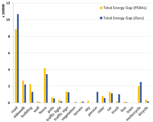
(a)

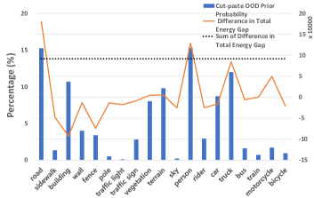
(b)

Figure 2: Analysis results of our method in the semantic segmentation task (Fishyscapes Lost&Found validation set) (a): Comparison of the class-wise total energy gap of PEBAL and our method; (b): class-wise total energy gap difference between PEBAL and our method.

We define the novel term Energy Gap as $\mathbb{E}[E(x_{in})]-\mathbb{E}[E(x_{out})]$, which measures the average energy gap between ID data and OOD data. We can measure it class-wise and $i$ th class Energy Gap is $\mathbb{E}[E(x_{in,i})]-\mathbb{E}[E(x_{out,i})]$. Finally, the class-wise Total Energy Gap is defined as $(\mathbb{E}[E(x_{in,i})]-\mathbb{E}[E(x_{out,i})])\cdot N_{out,i}$ by multiplying frequency of class $i$ OOD data. Intuitively, the larger the Total Energy Gap, the larger the energy gap between ID and OOD, and the better the OOD detection performance. Figure 2(a) compares the results of our method and PEBAL with regard to the class-wise Total Energy Gap. We see that this gap is elevated in the majority class, like the road.

Figure 2(b) shows the difference in Total Energy Gap between PEBAL and ours. As shown in Figure 2(b), class-wise difference distribution shown in orange is similar to the prior probability shown in blue, which infers that our balanced energy regularization effectively works. Furthermore, by improving the gap on the majority class effectively, the sum of the class-wise Total Energy Gap increases (black dotted line is over 0). Thus, our method improves the OOD detection performance compared to PEBAL.

5.2 Ablation Study

5.2.1 Hyperparameter Analysis

Table 7: Evaluation result in semantic segmentation task depending on $\gamma$ : OOD detection performance(AUROC,AP,FPR) and accuracy(MIOU for Cityscapes validation) on the Fishyscapes validation sets

Method City FS Lost & Found FS Static Name $\gamma$ MIOU$\uparrow$ AUC$\uparrow$ AP$\uparrow$ FPR$\downarrow$ AUC$\uparrow$ AP$\uparrow$ FPR$\downarrow$ EnergyOE 0.0 89.07 98.14 45.61 8.21 99.32 89.12 2.62 Balanced EnergyOE 1.0 89.04 98.01 50.42 8.87 99.34 89.28 2.33 2.0 89.83 98.72 53.36 6.57 99.42 90.32 2.31 3.0 88.91 98.42 54.58 6.70 99.43 91.77 1.63 4.0 88.53 98.81 53.27 5.18 99.34 89.98 2.39 Inverse Balanced EnergyOE -3.0 84.28 95.49 43.94 31.28 98.45 81.32 5.66

Table 8: Evaluation result on CIFAR10-LT depending on $\gamma$ :average (over 6 datasets) OOD detection performance (AUROC,AP, FPR) and classification accuracy (ACC) with model ResNet18; Mean over six random runs are reported.

Method		ACC$\uparrow$	Average (total 6)
Name	$\gamma$		AUC$\uparrow$	AP$\uparrow$	FPR$\downarrow$
Energy OE	0.00	74.53	91.92	91.97	33.79
Balanced Energy OE	0.10	75.03	92.01	91.57	32.80
	0.25	75.23	92.16	91.36	31.83
	0.50	75.92	92.44	91.67	30.81
	0.75	76.22	92.56	91.94	30.60
	1.00	74.85	92.45	92.03	31.86
	1.25	72.38	92.33	92.03	32.60
Inv-Balanced Energy OE	-0.75	64.24	90.75	90.83	39.82

As discussed in Section 3.2, the hyperparameter $\gamma$ controls the degree of prior difference between classes. We fix $\alpha$ as in Table 1 and find the best $\gamma$ starting from base case of $\gamma=0$. For accurate implementation of baseline EnergyOE, we only set $\alpha=0$, when $\gamma=0$. For semantic segmentation task and long-tailed image classification task as in Table 7 and Table 8, we obtain a common tendency for $\gamma$. First, as $\gamma$ becomes larger than 0, the OOD detection performance and accuracy improves, then obtain an optimal value and decrease again. Second, in the inverse case where $\gamma$ becomes smaller than 0, both OOD detection performance and accuracy are worse than the baseline. This would be evidence of the efficiency of prior probability.

5.2.2 Loss Component Analysis

Table 9: Results of the loss component ablation on Fishyscapes validation sets in semantic segmentation task

Loss Component		FS Lost & Found			FS Static
Margin	Weight	AUC$\uparrow$	AP$\uparrow$	FPR$\downarrow$	AUC$\uparrow$	AP$\uparrow$	FPR$\downarrow$
✗	✗	98.14	45.61	8.21	99.32	89.12	2.62
✗	✓	98.31	47.10	7.04	99.34	89.73	2.31
✓	✗	98.46	51.65	7.17	99.41	90.14	2.23
✓	✓	98.42	54.58	6.70	99.43	91.77	1.63

Table 10: Results of the loss component ablation on both CIFAR10-LT and CIFAR100-LT in long-tailed image classification task

Loss Component		CIFAR10-LT Average			CIFAR100-LT Average
Margin	Weight	AUC$\uparrow$	AP$\uparrow$	FPR$\downarrow$	AUC$\uparrow$	AP$\uparrow$	FPR$\downarrow$
✗	✗	91.92	91.97	33.79	76.40	72.24	64.54
✗	✓	92.32	91.39	31.00	77.28	72.20	61.92
✓	✗	92.32	92.27	32.44	77.17	72.99	63.23
✓	✓	92.56	91.94	30.60	77.75	73.10	61.15

As defined in Section 3.2, our balanced energy regularization loss has two adaptive loss components that depend on $Z_{\gamma}$. For the semantic segmentation task and long-tailed image classification task as in Table 9 and Table 10, ablation results on two loss components show that we can achieve the best performance when using both adaptive loss margin and adaptive loss weight.

5.2.3 Network Analysis

Table 11: Evaluation result on long-tailed CIFAR using WideResNet(WRN-40-2); average (over 6 datasets) OOD detection performance (AUROC,AP, FPR) and classification accuracy (ACC) (a): Result on CIFAR10-LT (b): Result on CIFAR100-LT

(a)

Dataset	Method	AUC$\uparrow$	AP$\uparrow$	FPR$\downarrow$	ACC$\uparrow$
Average	MSP [17](ST)	74.59	72.62	63.96	72.32
	Energy [29](ST)	80.23	77.67	58.44	72.32
	OE [18](tune)	83.96	83.70	54.60	69.31
	EnergyOE [29](tune)	91.44	91.01	34.02	75.02
	Ours	91.85	90.48	31.03	76.14

(b)

Dataset	Method	AUC$\uparrow$	AP$\uparrow$	FPR$\downarrow$	ACC$\uparrow$
Average	MSP [17](ST)	60.24	57.22	83.52	40.96
	Energy [29](ST)	63.31	59.44	81.95	40.96
	OE [18](tune)	68.52	65.18	76.88	41.73
	EnergyOE [29](tune)	76.45	72.75	65.70	39.95
	Ours	77.41	73.10	62.84	39.44

To show the generality of our method, we perform a long-tailed image classification experiment on WideResNet (WRN-40-2) [48] instead of ResNet18 [14]. When $\gamma$ is 0.5 ($\alpha$ as in Table 1), we get optimal performance in both CIFAR10-LT and CIFAR100-LT, and the results are as summarized in Table 11(b) and Table 11(b), respectively. Our approach outperforms the current baselines (OE, EnergyOE) on both CIFAR10-LT and CIFAR100-LT, similar to the case with ResNet18.

6 Conclusion

To solve the OOD detection issue in various tasks, we propose a new balanced energy regularization loss. The main idea of our loss is to apply large regularization to auxiliary samples of majority classes, compared to those of minority. We show the effectiveness of our novel loss through extensive experiments on semantic segmentation, long-tailed image classification, and image classification datasets. Limitations and potential negative social impacts are provided in the supplement.

Supplementary Material

S.1 Limitations

Although our method is a simple and competitive approach to various OOD detection tasks, additional auxiliary data is still required. OOD detection without additional data would be an ideal model. However, approaches that use auxiliary data still show superior performance to the approaches without using auxiliary data. Instead, we can consider a way to utilize a small amount of auxiliary data as little as possible with competitive performance in future work.

S.2 Potential Negative Societal Impacts

OOD detection is a branch of anomaly detection. In vision tasks, anomaly detection typically plays a positive role in strengthening security in surveillance systems. However, indiscriminate abuse of automated surveillance systems can increase the surveillance of workers. Therefore, when our method is applied to a real environment, we ensure ours to be used only for the purpose of enhancing human safety without infringing on human privacy.

S.3 Further details of implementation

For Section 4.1.3, we add a bit more to our implementation, In long-tailed image classification, fine-tuning-based methods OE [18], OECC [38], EnergyOE [29], and ours are trained for 20 epochs on both CIFAR10-LT and CIFAR100-LT. For OECC, we set the coefficients to $\lambda_{1}=\lambda_{2}=0.03$.

In image classification, the number of training epochs mostly follows the conventional method. Therefore, in OE it is set to 10 for both CIFAR10 and CIFAR100, and in OECC it is set to 15 for both. For OECC, we set the coefficients to $\lambda_{1}=0.07$ and $\lambda_{2}=0.05$. On the other hand, we found that the convergence of training is fast when using our balanced energy regularization loss, unlike the conventional method. Therefore, we set the number of training epochs to 8 for CIFAR10 and the number of training epochs to 4 for CIFAR100 to get the optimal OOD detection performance. Therefore, we also report the results of EnergyOE with the same number of epochs as 8 for CIFAR10 and 4 for CIFAR100 for fair comparison with our loss. For reference, results of EnergyOE for training 10 epochs as in the original work are 96.56, 96.37, 15.27, and 93.29 for CIFAR10 in the order of AUROC, AP, FPR, and ACC. For CIFAR100, we get 85.56, 80.68, 43.64, and 74.92. Still, the comparison in Table 6 confirms the superiority of our method.

S.4 Details on the setting of hyperparameter $\alpha$

As discussed in Section 3.2, we set the adaptive loss margin as $\alpha$$\cdot$$Z_{\gamma}$. More specifically, to standardize $\alpha$, we redesign $\alpha$ as a relative offset from the baseline which the case of $\gamma$=$0$. Thus, we set $\alpha\approx\beta$$\cdot$$K$$\cdot$ ($m_{out}-m_{in}$), where $\beta$ is proportionality constant, $K$ is a number of classes and $m_{out}-m_{in}$ is energy distance between in-distribution and OOD, respectively. When $\gamma$=$0$, adaptive loss margin $\alpha$$\cdot$$Z_{\gamma}$ become $\beta$$\cdot$ ($m_{out}-m_{in}$), which is the relative offset proportional to $\beta$. As $\beta$ increases, the sensitivity to $\gamma$ increases, and even a small change in $\gamma$ greatly changes the adaptive loss margin. Conversely, if we set $\beta$$\approx$$0$, the sensitivity to $\gamma$ becomes small, and even if $\gamma$ increases, the adaptive margin approaches 0 regardless of this, so there is no difference from the original energy regularization loss $L_{out,hinge}$. Finally, we choose to use the appropriate $\beta=0.05$ with corresponding $\alpha$ and adjust the hyperparameter $\gamma$. As seen in Table S.1 and Table S.2, AUROC and accuracy also show similar tendencies as discussed above.

Table S.1: Average AUROC (over 6 datasets) on CIFAR10-LT using ResNet18 depending on hyperparameter $\gamma$ and $\alpha$

Average AUROC
Hyperparameter $\gamma$	Hyperparameter $\beta$
	0.0025	0.01	0.025	0.05	0.1	0.25	0.5
	Hyperparameter $\alpha$
	0.5	2	5	10	20	50	100
0.1	91.92	91.93	91.98	92.01	92.12	92.02	91.52
0.25	91.96	92.00	92.07	92.16	92.28	92.42	91.69
0.5	92.17	92.20	92.29	92.44	92.55	92.11	91.85
0.75	92.34	92.39	92.48	92.56	92.50	92.00	91.82
1	92.41	92.47	92.52	92.45	92.44	91.91	91.79
1.25	92.39	92.41	92.37	92.33	92.27	91.94	91.61

Table S.2: Accuracy on CIFAR10-LT using ResNet18 depending on hyperparameter $\gamma$ and $\alpha$

Accuracy(ACC)
Hyperparameter $\gamma$	Hyperparameter $\beta$
	0.0025	0.01	0.025	0.05	0.1	0.25	0.5
	Hyperparameter $\alpha$
	0.5	2	5	10	20	50	100
0.1	74.53	74.60	74.84	75.03	75.45	73.71	70.18
0.25	74.57	74.64	74.86	75.23	75.95	76.13	63.15
0.5	75.15	75.23	75.61	75.92	76.60	68.03	59.78
0.75	75.88	75.87	76.29	76.22	74.87	65.64	56.92
1	76.15	75.92	75.98	74.85	72.40	62.86	54.66
1.25	75.94	75.66	74.61	72.38	69.96	60.85	52.43

S.5 OOD prior probability for all tasks

S.5.1 Semantic Segmentation

Table S.3: OOD prior probability in semantic segmentation task: cut-pasted OOD pixel inference result collected from 10000 synthesized scene images

class index	0	1	2	3	4	5	6	7	8	9
class name	road	sidewalk	building	wall	fence	pole	traffic light	traffic sign	vegetation	terrain
probability	1.53E-01	1.33E-02	1.07E-01	4.01E-02	3.39E-02	5.26E-03	1.06E-03	2.80E-02	8.02E-02	9.80E-02
class index	10	11	12	13	14	15	16	17	18
class name	sky	person	rider	car	truck	bus	train	motorcycle	bicycle
probability	2.17E-03	1.53E-01	2.92E-02	8.71E-02	1.20E-01	1.60E-02	7.07E-03	1.70E-02	9.39E-03

S.5.2 Long-tailed Image Classification

Table S.4: OOD prior probability in long-tailed image classification task: TinyImages 300K inference result on CIFAR10-LT model using ResNet18 :

class index	0	1	2	3	4	5	6	7	8	9
class name	airplane	automobile	bird	cat	deer	dog	frog	horse	ship	truck
probability	2.50E-01	7.96E-02	1.63E-01	2.49E-01	6.15E-02	8.50E-02	3.05E-02	2.32E-02	2.39E-02	3.45E-02

Table S.5: OOD prior probability in long-tailed image classification task: TinyImages 300K inference result on CIFAR100-LT model using ResNet18

class index	0	1	2	3	4	5	6	7	8	9
class name	apple	aquarium_fish	baby	bear	beaver	bed	bee	beetle	bicycle	bottle
probability	7.58E-03	1.69E-02	6.16E-02	2.54E-02	1.78E-02	3.67E-02	2.81E-02	1.02E-02	1.87E-02	3.70E-02
class index	10	11	12	13	14	15	16	17	18	19
class name	bowl	boy	bridge	bus	butterfly	camel	can	castle	caterpillar	cattle
probability	2.98E-02	6.17E-02	3.48E-02	4.20E-02	1.69E-02	1.61E-02	6.56E-02	2.40E-02	2.52E-02	1.70E-02
class index	20	21	22	23	24	25	26	27	28	29
class name	chair	chimpanzee	clock	cloud	cockroach	couch	crab	crocodile	cup	dinosaur
probability	7.81E-03	7.30E-03	2.55E-02	1.84E-02	3.27E-03	2.78E-02	9.09E-03	1.17E-02	7.72E-03	9.21E-03
class index	30	31	32	33	34	35	36	37	38	39
class name	dolphin	elephant	flatfish	forest	fox	girl	hamster	house	kangaroo	keyboard
probability	8.08E-03	7.00E-03	9.30E-03	2.38E-02	3.79E-03	1.99E-02	4.01E-03	1.64E-02	6.19E-03	1.74E-02
class index	40	41	42	43	44	45	46	47	48	49
class name	lamp	lawn_mower	leopard	lion	lizard	lobster	man	maple_tree	motorcycle	mountain
probability	1.59E-02	6.44E-03	7.91E-03	2.53E-03	6.93E-03	7.94E-03	1.97E-02	4.40E-03	3.35E-03	8.74E-03
class index	50	51	52	53	54	55	56	57	58	59
class name	mouse	mushroom	oak_tree	orange	orchid	otter	palm_tree	pear	pickup_truck	pine_tree
probability	2.52E-03	4.93E-03	1.88E-03	2.78E-03	5.78E-03	1.05E-03	2.04E-03	1.31E-03	2.52E-03	2.38E-03
class index	60	61	62	63	64	65	66	67	68	69
class name	plain	plate	poppy	porcupine	possum	rabbit	raccoon	ray	road	rocket
probability	1.14E-02	1.46E-02	3.08E-03	1.42E-03	4.73E-03	7.11E-03	3.10E-03	5.36E-03	4.87E-03	9.77E-03
class index	70	71	72	73	74	75	76	77	78	79
class name	rose	sea	seal	shark	shrew	skunk	skyscraper	snail	snake	spider
probability	1.94E-03	3.22E-03	4.47E-04	9.43E-04	2.63E-04	3.23E-04	2.14E-03	1.33E-04	1.59E-03	8.27E-04
class index	80	81	82	83	84	85	86	87	88	89
class name	squirrel	streetcar	sunflower	sweet_pepper	table	tank	telephone	television	tiger	tractor
probability	2.10E-04	1.89E-03	1.05E-03	4.87E-04	1.35E-03	3.57E-04	1.10E-03	3.32E-03	4.07E-04	2.84E-03
class index	90	91	92	93	94	95	96	97	98	99
class name	train	trout	tulip	turtle	wardrobe	whale	willow_tree	wolf	woman	worm
probability	7.27E-04	7.00E-05	9.33E-05	2.00E-05	2.87E-03	1.60E-04	2.43E-04	5.33E-05	4.03E-04	9.00E-05

S.5.3 Image Classification

Table S.6: OOD prior probability in image classification task: TinyImages 300K inference result on CIFAR10 model using ResNet18

class index	0	1	2	3	4	5	6	7	8	9
class name	airplane	automobile	bird	cat	deer	dog	frog	horse	ship	truck
probability	1.15E-01	3.62E-02	9.94E-02	2.04E-01	3.58E-02	1.19E-01	7.51E-02	5.35E-02	9.91E-02	1.62E-01

Table S.7: OOD prior probability in image classification task: TinyImages 300K inference result on CIFAR100 model using ResNet18.

class index	0	1	2	3	4	5	6	7	8	9
class name	apple	aquarium_fish	baby	bear	beaver	bed	bee	beetle	bicycle	bottle
probability	1.39E-03	1.60E-03	1.50E-02	6.34E-03	2.66E-03	1.15E-02	3.01E-03	2.50E-03	5.32E-03	1.88E-02
class index	10	11	12	13	14	15	16	17	18	19
class name	bowl	boy	bridge	bus	butterfly	camel	can	castle	caterpillar	cattle
probability	1.98E-02	1.97E-02	1.69E-02	1.36E-02	4.82E-03	5.97E-03	4.14E-02	1.24E-02	9.66E-03	1.01E-02
class index	20	21	22	23	24	25	26	27	28	29
class name	chair	chimpanzee	clock	cloud	cockroach	couch	crab	crocodile	cup	dinosaur
probability	7.11E-03	4.63E-03	2.11E-02	1.93E-02	2.88E-03	2.62E-02	4.44E-03	4.88E-03	7.81E-03	3.48E-03
class index	30	31	32	33	34	35	36	37	38	39
class name	dolphin	elephant	flatfish	forest	fox	girl	hamster	house	kangaroo	keyboard
probability	1.46E-03	5.00E-03	1.37E-02	2.69E-02	2.08E-03	1.68E-02	1.25E-03	2.83E-02	4.45E-03	2.18E-02
class index	40	41	42	43	44	45	46	47	48	49
class name	lamp	lawn_mower	leopard	lion	lizard	lobster	man	maple_tree	motorcycle	mountain
probability	2.38E-02	5.93E-03	3.82E-03	9.67E-04	9.30E-03	1.61E-02	7.35E-02	2.05E-03	8.32E-03	6.84E-03
class index	50	51	52	53	54	55	56	57	58	59
class name	mouse	mushroom	oak_tree	orange	orchid	otter	palm_tree	pear	pickup_truck	pine_tree
probability	3.60E-03	6.78E-03	8.63E-04	3.11E-03	1.05E-02	5.41E-03	3.04E-03	5.48E-03	6.31E-03	9.94E-03
class index	60	61	62	63	64	65	66	67	68	69
class name	plain	plate	poppy	porcupine	possum	rabbit	raccoon	ray	road	rocket
probability	1.14E-02	1.46E-02	3.08E-03	1.42E-03	4.73E-03	7.11E-03	3.10E-03	5.36E-03	4.87E-03	9.77E-03
class index	70	71	72	73	74	75	76	77	78	79
class name	rose	sea	seal	shark	shrew	skunk	skyscraper	snail	snake	spider
probability	4.86E-03	1.47E-02	4.44E-03	5.88E-03	1.82E-03	2.13E-03	8.50E-03	2.21E-03	8.53E-03	5.92E-03
class index	80	81	82	83	84	85	86	87	88	89
class name	squirrel	streetcar	sunflower	sweet_pepper	table	tank	telephone	television	tiger	tractor
probability	4.27E-03	1.23E-02	3.71E-03	9.63E-03	3.25E-02	1.06E-02	1.38E-02	2.93E-02	3.31E-03	1.12E-02
class index	90	91	92	93	94	95	96	97	98	99
class name	train	trout	tulip	turtle	wardrobe	whale	willow_tree	wolf	woman	worm
probability	8.04E-03	2.99E-03	6.48E-03	2.52E-03	2.10E-02	2.42E-03	9.76E-03	3.52E-03	2.64E-02	1.00E-02

S.6 Detailed Experiment Results

S.6.1 Semantic Segmentation

Table S.8: Detailed evaluation result in semantic segmentation task depending on $\gamma$ : OOD detection performance(AUROC,AP,FPR) and accuracy(MIOU for Cityscapes validation) on the Fishyscapes validation sets and Road Anomaly test set

Method		City	FS Lost & Found			FS Static			Road Anomaly
Name	$\gamma$	MIOU$\uparrow$	AUC$\uparrow$	AP$\uparrow$	FPR$\downarrow$	AUC$\uparrow$	AP$\uparrow$	FPR$\downarrow$	AUC$\uparrow$	AP$\uparrow$	FPR$\downarrow$
EnergyOE	0.0	89.07	98.14	45.61	8.21	99.32	89.12	2.62	83.32	32.59	53.01
Balanced EnergyOE	1.0	89.04	98.01	50.42	8.87	99.34	89.28	2.33	83.61	30.73	49.96
	2.0	89.83	98.72	53.36	6.57	99.42	90.32	2.31	84.90	33.72	46.39
	3.0	88.91	98.42	54.58	6.70	99.43	91.77	1.63	85.50	34.90	46.60
	4.0	88.53	98.81	53.27	5.18	99.34	89.98	2.39	83.53	29.51	46.91
Inverse Balanced EnergyOE	-3.0	84.28	95.49	43.94	31.28	98.45	81.32	5.66	84.92	41.17	55.57

S.6.2 Long-tailed Image Classification

ResNet18 model on CIFAR10-LT:

Table S.9: Detailed evaluation result on CIFAR10-LT depending on $\gamma$ : OOD detection performance (AUROC,AP, FPR) and classification accuracy (ACC) with model ResNet18; Mean over six random runs are reported; (a): ACC and result on Texture, SVHN, and CIFAR100; (b): Total average result and result on Tiny Imagenet, LSUN, and Place365

(a)

Method		ACC$\uparrow$	Texture			SVHN			CIFAR 100
Name	$\gamma$		AUC$\uparrow$	AP$\uparrow$	FPR$\downarrow$	AUC$\uparrow$	AP$\uparrow$	FPR$\downarrow$	AUC$\uparrow$	AP$\uparrow$	FPR$\downarrow$
Energy OE	0.00	74.53	95.53	92.93	23.26	96.63	98.46	14.52	84.44	84.63	59.92
Balanced Energy OE	0.10	75.03	95.49	91.94	22.44	96.68	97.90	12.64	84.63	84.42	59.16
	0.25	75.23	95.55	91.63	22.03	96.99	98.06	11.82	84.89	84.40	57.80
	0.50	75.92	95.70	92.05	21.13	97.49	98.63	10.48	85.18	84.78	57.09
	0.75	76.22	95.69	92.38	21.26	97.74	98.89	9.87	85.20	84.98	57.95
	1.00	74.85	95.56	92.57	22.57	97.94	99.03	9.11	84.84	84.90	61.18
	1.25	72.38	95.42	92.67	23.92	98.10	99.09	8.86	84.45	84.61	62.15
Inv-Balanced Energy OE	-0.75	64.24	95.19	92.14	27.52	96.59	98.48	18.89	81.76	81.91	63.45

(b)

Method	Tiny ImageNet			LSUN			Place365			Average
$\gamma$	AUC$\uparrow$	AP$\uparrow$	FPR$\downarrow$	AUC$\uparrow$	AP$\uparrow$	FPR$\downarrow$	AUC$\uparrow$	AP$\uparrow$	FPR$\downarrow$	AUC$\uparrow$	AP$\uparrow$	FPR$\downarrow$
0.00	88.40	84.95	45.17	94.00	93.70	26.96	92.51	97.14	32.88	91.92	91.97	33.79
0.10	88.51	84.58	44.56	94.12	93.49	26.36	92.67	97.10	31.61	92.01	91.57	32.80
0.25	88.63	84.37	43.29	94.12	92.72	25.52	92.79	96.98	30.54	92.16	91.36	31.83
0.50	88.85	84.71	42.46	94.30	92.80	24.62	93.10	97.08	29.11	92.44	91.67	30.81
0.75	88.92	84.98	42.38	94.48	93.15	23.88	93.35	97.23	28.25	92.56	91.94	30.60
1.00	88.74	85.06	43.11	94.36	93.35	25.71	93.26	97.27	29.46	92.45	92.03	31.86
1.25	88.47	84.95	44.07	94.31	93.56	26.46	93.24	97.30	30.15	92.33	92.03	32.60
-0.75	86.70	82.96	50.86	93.10	92.86	36.08	91.14	96.62	42.15	90.75	90.83	39.82

Table S.10: Detailed evaluation result on CIFAR10-LT depending on $\gamma$ : OOD detection performance (AUROC,AP, FPR) and classification accuracy (ACC) with model ResNet18; Std over six random runs are reported; (a): ACC and result on Texture, SVHN, and CIFAR100; (b): Total average result and result on Tiny Imagenet, LSUN, and Place365

(a)

Method		ACC$\uparrow$	Texture			SVHN			CIFAR 100
Name	$\gamma$		AUC$\uparrow$	AP$\uparrow$	FPR$\downarrow$	AUC$\uparrow$	AP$\uparrow$	FPR$\downarrow$	AUC$\uparrow$	AP$\uparrow$	FPR$\downarrow$
Energy OE	0.00	3.09E-02	3.73E-03	8.98E-03	1.43E-01	3.82E-02	1.89E-02	1.14E-01	5.00E-03	5.00E-03	8.22E-02
Balanced Energy OE	0.10	2.63E-02	5.00E-03	1.11E-02	8.76E-02	2.97E-02	1.89E-02	1.52E-01	7.64E-03	9.43E-03	1.59E-01
	0.25	4.75E-02	6.87E-03	1.49E-02	8.96E-02	1.97E-02	1.73E-02	1.03E-01	1.00E-02	1.15E-02	8.42E-02
	0.50	4.83E-02	5.77E-03	2.13E-02	5.93E-02	1.61E-02	8.16E-03	8.55E-02	6.87E-03	1.29E-02	1.37E-01
	0.75	3.73E-02	8.98E-03	2.71E-02	1.30E-01	9.57E-03	6.87E-03	1.15E-01	5.77E-03	1.29E-02	1.79E-01
	1.00	5.15E-02	6.87E-03	2.21E-02	1.51E-01	1.41E-02	6.87E-03	9.36E-02	7.64E-03	8.98E-03	1.22E-01
	1.25	4.12E-02	1.07E-02	2.69E-02	1.13E-01	2.52E-02	1.49E-02	9.93E-02	8.98E-03	9.43E-03	1.28E-01
Inv-Balanced Energy OE	-0.75	4.89E-02	4.71E-03	7.45E-03	1.22E-01	2.11E-02	1.26E-02	1.39E-01	4.71E-03	4.71E-03	9.64E-02

(b)

Method	Tiny ImageNet			LSUN			Place365			Average
$\gamma$	AUC$\uparrow$	AP$\uparrow$	FPR$\downarrow$	AUC$\uparrow$	AP$\uparrow$	FPR$\downarrow$	AUC$\uparrow$	AP$\uparrow$	FPR$\downarrow$	AUC$\uparrow$	AP$\uparrow$	FPR$\downarrow$
0.00	5.00E-03	3.73E-03	1.03E-01	9.43E-03	9.57E-03	5.35E-02	3.73E-03	0.00E+00	6.47E-02	1.08E-02	7.70E-03	9.34E-02
0.10	9.57E-03	6.87E-03	1.46E-01	3.73E-03	8.98E-03	9.69E-02	5.00E-03	5.00E-03	6.59E-02	1.01E-02	1.00E-02	1.18E-01
0.25	5.00E-03	1.34E-02	3.65E-02	1.15E-02	1.26E-02	9.09E-02	8.16E-03	5.00E-03	7.69E-02	1.02E-02	1.25E-02	8.01E-02
0.50	3.73E-03	8.98E-03	5.21E-02	6.87E-03	1.21E-02	6.88E-02	7.45E-03	4.71E-03	5.98E-02	7.80E-03	1.14E-02	7.71E-02
0.75	1.11E-02	1.07E-02	1.16E-01	7.64E-03	1.34E-02	7.16E-02	4.71E-03	5.00E-03	1.38E-01	7.96E-03	1.27E-02	1.25E-01
1.00	7.64E-03	1.70E-02	4.16E-02	1.29E-02	1.89E-02	1.59E-01	4.71E-03	5.00E-03	4.74E-02	8.99E-03	1.31E-02	1.03E-01
1.25	9.43E-03	1.11E-02	6.99E-02	5.77E-03	8.98E-03	1.84E-01	5.00E-03	3.73E-03	5.43E-02	1.08E-02	1.25E-02	1.08E-01
-0.75	3.73E-03	6.87E-03	1.47E-01	3.73E-03	5.77E-03	7.29E-02	3.73E-03	5.00E-03	7.57E-02	6.96E-03	7.07E-03	1.09E-01

ResNet18 model on CIFAR100-LT:

Table S.11: Detailed evaluation result on CIFAR100-LT depending on $\gamma$ : OOD detection performance (AUROC,AP, FPR) and classification accuracy (ACC) with model ResNet18; Mean over six random runs are reported; (a): ACC and result on Texture, SVHN, and CIFAR10; (b): Total average result and result on Tiny Imagenet, LSUN, and Place365

(a)

Method		ACC$\uparrow$	Texture			SVHN			CIFAR 10
Name	$\gamma$		AUC$\uparrow$	AP$\uparrow$	FPR$\downarrow$	AUC$\uparrow$	AP$\uparrow$	FPR$\downarrow$	AUC$\uparrow$	AP$\uparrow$	FPR$\downarrow$
Energy OE	0.00	40.65	79.56	70.88	68.60	86.19	91.74	42.27	61.15	56.66	82.60
Balanced Energy OE	0.10	40.90	79.78	70.80	68.01	86.65	91.93	41.01	61.29	56.65	82.19
	0.25	41.50	80.06	69.91	66.93	86.91	91.99	39.46	61.24	56.51	82.23
	0.50	41.64	81.01	70.87	65.50	87.45	92.15	36.93	61.38	55.73	83.49
	0.75	41.05	82.10	73.09	64.19	88.66	92.88	33.79	59.40	54.97	85.16
	1.00	38.62	83.28	75.67	63.54	89.68	93.71	32.64	58.81	54.60	86.46
	1.25	36.51	84.33	77.49	62.14	90.71	94.48	30.90	58.29	54.30	87.42
Inv-Balanced Energy OE	-0.75	34.77	82.79	77.96	70.45	83.12	90.07	51.32	58.34	54.32	88.17

(b)

Method	Tiny ImageNet			LSUN			Place365			Average
$\gamma$	AUC$\uparrow$	AP$\uparrow$	FPR$\downarrow$	AUC$\uparrow$	AP$\uparrow$	FPR$\downarrow$	AUC$\uparrow$	AP$\uparrow$	FPR$\downarrow$	AUC$\uparrow$	AP$\uparrow$	FPR$\downarrow$
0.00	70.78	55.90	74.43	81.61	69.16	57.37	79.12	89.09	61.96	76.40	72.24	64.54
0.10	70.89	55.85	74.23	81.94	69.37	56.53	79.42	89.18	60.93	76.66	72.29	63.82
0.25	71.10	55.85	74.12	82.35	69.55	55.50	79.86	89.31	59.54	76.92	72.18	62.96
0.50	71.36	56.15	73.81	83.25	70.48	52.87	80.65	89.65	58.09	77.35	72.50	61.78
0.75	71.42	56.52	74.22	83.83	71.23	52.04	81.10	89.94	57.52	77.75	73.10	61.15
1.00	71.41	56.76	75.08	83.76	71.40	53.46	81.12	90.09	58.79	78.01	73.70	61.66
1.25	71.38	56.81	75.18	82.85	70.92	58.68	80.17	89.83	64.16	77.96	73.97	63.08
-0.75	69.27	55.59	77.09	80.20	68.79	66.63	77.09	88.64	70.64	75.14	72.56	70.71

Table S.12: Detailed evaluation result on CIFAR100-LT depending on $\gamma$ : OOD detection performance (AUROC,AP, FPR) and classification accuracy (ACC) with model ResNet18; Std over six random runs are reported; (a): ACC and result on Texture, SVHN, and CIFAR10; (b): Total average result and result on Tiny Imagenet, LSUN, and Place365

(a)

Method		ACC$\uparrow$	Texture			SVHN			CIFAR 10
Name	$\gamma$		AUC$\uparrow$	AP$\uparrow$	FPR$\downarrow$	AUC$\uparrow$	AP$\uparrow$	FPR$\downarrow$	AUC$\uparrow$	AP$\uparrow$	FPR$\downarrow$
Energy OE	0.00	1.63E-02	3.73E-03	1.25E-02	4.22E-02	2.03E-02	1.41E-02	4.07E-02	4.71E-03	3.73E-03	2.93E-02
Balanced Energy OE	0.10	2.48E-02	1.12E-02	2.29E-02	6.19E-02	1.53E-02	1.11E-02	4.23E-02	0.00E+00	4.71E-03	2.92E-02
	0.25	2.91E-02	3.73E-03	6.87E-03	6.47E-02	1.86E-02	1.77E-02	8.08E-02	4.71E-03	5.00E-03	2.99E-02
	0.50	2.48E-02	9.57E-03	1.71E-02	5.16E-02	2.27E-02	1.61E-02	4.81E-02	4.71E-03	5.00E-03	4.36E-02
	0.75	3.64E-02	7.45E-03	1.25E-02	1.09E-01	1.95E-02	1.41E-02	2.11E-02	3.73E-03	3.73E-03	3.09E-02
	1.00	3.35E-02	9.43E-03	8.98E-03	1.06E-01	2.21E-02	1.38E-02	1.36E-01	5.77E-03	3.73E-03	4.35E-02
	1.25	3.83E-02	9.43E-03	1.15E-02	4.99E-02	2.13E-02	1.89E-02	8.65E-02	7.64E-03	9.57E-03	4.35E-02
Inv-Balanced Energy OE	-0.75	2.31E-02	4.71E-03	4.71E-03	2.81E-02	2.00E-02	1.26E-02	7.39E-02	7.11E-15	4.71E-03	2.08E-02

(b)

Method	Tiny ImageNet			LSUN			Place365			Average
$\gamma$	AUC$\uparrow$	AP$\uparrow$	FPR$\downarrow$	AUC$\uparrow$	AP$\uparrow$	FPR$\downarrow$	AUC$\uparrow$	AP$\uparrow$	FPR$\downarrow$	AUC$\uparrow$	AP$\uparrow$	FPR$\downarrow$
0.00	1.42E-14	4.71E-03	4.41E-02	0.00E+00	4.71E-03	9.09E-02	0.00E+00	1.42E-14	4.12E-02	4.80E-03	6.63E-03	4.81E-02
0.10	0.00E+00	3.73E-03	3.59E-02	5.00E-03	4.71E-03	8.35E-02	0.00E+00	5.00E-03	3.53E-02	5.24E-03	8.68E-03	4.80E-02
0.25	4.71E-03	4.71E-03	4.34E-02	3.73E-03	3.73E-03	4.14E-02	4.71E-03	3.73E-03	1.63E-02	6.70E-03	6.96E-03	4.61E-02
0.50	0.00E+00	4.71E-03	5.58E-02	4.71E-03	3.73E-03	6.15E-02	5.00E-03	3.73E-03	6.74E-02	7.78E-03	8.39E-03	5.47E-02
0.75	3.73E-03	6.87E-03	6.52E-02	0.00E+00	5.00E-03	7.91E-02	4.71E-03	5.00E-03	4.26E-02	6.52E-03	7.87E-03	5.80E-02
1.00	6.87E-03	1.07E-02	3.50E-02	5.77E-03	6.87E-03	4.78E-02	3.73E-03	4.71E-03	5.89E-02	8.95E-03	8.13E-03	7.11E-02
1.25	4.71E-03	4.71E-03	6.08E-02	1.07E-02	1.11E-02	3.73E-02	7.45E-03	0.00E+00	5.55E-02	1.02E-02	9.30E-03	5.56E-02
-0.75	0.00E+00	4.71E-03	2.67E-02	5.77E-03	6.87E-03	2.63E-02	4.71E-03	0.00E+00	3.89E-02	5.87E-03	5.60E-03	3.58E-02

WideResNet model on CIFAR10-LT:

Table S.13: Detailed evaluation result on CIFAR10-LT depending on $\gamma$ : OOD detection performance (AUROC,AP, FPR) and classification accuracy (ACC) with model WideResNet(WRN-40-2); Mean over six random runs are reported; (a): ACC and result on Texture, SVHN, and CIFAR100; (b): Total average result and result on Tiny Imagenet, LSUN, and Place365

(a)

Method		ACC$\uparrow$	Texture			SVHN			CIFAR 100
Name	$\gamma$		AUC$\uparrow$	AP$\uparrow$	FPR$\downarrow$	AUC$\uparrow$	AP$\uparrow$	FPR$\downarrow$	AUC$\uparrow$	AP$\uparrow$	FPR$\downarrow$
Energy OE	0.00	75.03	94.25	89.94	26.79	95.07	96.66	16.08	84.20	84.00	57.71
Balanced Energy OE	0.10	75.28	94.39	89.27	25.82	95.22	96.34	14.76	84.39	83.81	56.63
	0.25	75.74	94.32	88.57	25.55	95.43	96.33	13.87	84.60	83.64	55.22
	0.50	76.14	94.31	88.39	26.08	95.83	96.73	12.75	84.80	83.81	54.68
	0.75	74.76	94.23	88.75	26.51	96.23	97.12	12.24	84.50	83.66	56.59
	1.00	71.20	94.14	89.77	29.40	96.51	97.74	12.56	84.00	83.50	58.40
	1.25	68.70	94.06	90.32	31.19	96.63	98.11	13.97	83.60	83.33	59.46
Inv-Balanced Energy OE	-0.75	62.91	93.15	90.49	39.41	94.22	97.22	24.63	80.54	80.87	65.46

(b)

Method	ACC$\uparrow$	Tiny ImageNet			LSUN			Place365			Average
$\gamma$		AUC$\uparrow$	AP$\uparrow$	FPR$\downarrow$	AUC$\uparrow$	AP$\uparrow$	FPR$\downarrow$	AUC$\uparrow$	AP$\uparrow$	FPR$\downarrow$	AUC$\uparrow$	AP$\uparrow$	FPR$\downarrow$
0.00	75.03	87.63	83.86	47.77	94.80	94.41	24.17	92.72	97.17	31.58	91.44	91.01	34.02
0.10	75.28	87.82	83.75	46.80	94.78	93.81	22.68	92.84	97.06	29.98	91.57	90.67	32.78
0.25	75.74	87.97	83.61	45.47	94.72	93.03	21.51	92.89	96.89	28.90	91.65	90.34	31.75
0.50	76.14	88.12	83.76	44.61	94.90	93.23	20.45	93.16	96.96	27.61	91.85	90.48	31.03
0.75	74.76	87.91	83.71	45.68	94.94	93.67	20.91	93.19	97.05	28.25	91.83	90.66	31.69
1.00	71.20	87.59	83.56	47.68	94.91	94.25	22.63	93.19	97.21	29.08	91.72	91.01	33.29
1.25	68.70	87.22	83.42	48.87	94.81	92.28	23.16	93.06	97.22	30.14	91.56	91.11	34.46
-0.75	62.91	84.81	81.26	56.31	92.93	92.66	36.62	90.38	96.35	44.05	89.34	89.81	44.41

Table S.14: Detailed evaluation result on CIFAR10-LT depending on $\gamma$ : OOD detection performance (AUROC,AP, FPR) and classification accuracy (ACC) with model WideResNet(WRN-40-2); Std over six random runs are reported; (a): ACC and result on Texture, SVHN, and CIFAR100; (b): Total average result and result on Tiny Imagenet, LSUN, and Place365

(a)

Method		ACC$\uparrow$	Texture			SVHN			CIFAR 100
Name	$\gamma$		AUC$\uparrow$	AP$\uparrow$	FPR$\downarrow$	AUC$\uparrow$	AP$\uparrow$	FPR$\downarrow$	AUC$\uparrow$	AP$\uparrow$	FPR$\downarrow$
Energy OE	0.00	4.92E-02	6.87E-03	1.26E-02	7.27E-02	1.49E-02	1.25E-02	5.34E-02	6.87E-03	6.87E-03	1.36E-01
Balanced Energy OE	0.10	3.80E-02	5.77E-03	1.63E-02	1.27E-01	1.34E-02	9.57E-03	4.35E-02	3.73E-03	3.73E-03	6.90E-02
	0.25	3.72E-02	9.43E-03	2.67E-02	1.34E-01	1.71E-02	1.73E-02	4.76E-02	5.77E-03	1.11E-02	7.86E-02
	0.50	4.74E-02	6.87E-03	4.20E-02	9.52E-02	1.80E-02	1.67E-02	7.24E-02	4.71E-03	1.61E-02	9.99E-02
	0.75	5.70E-02	9.43E-03	5.27E-02	1.56E-01	1.57E-02	1.57E-02	1.25E-01	1.11E-02	2.06E-02	2.15E-01
	1.00	6.52E-02	1.12E-02	4.56E-02	1.39E-01	1.71E-02	2.81E-02	1.66E-01	6.87E-03	1.95E-02	2.36E-01
	1.25	8.08E-02	2.48E-02	4.15E-02	1.65E-01	5.19E-02	4.11E-02	2.43E-01	1.70E-02	1.80E-02	1.47E-01
Inv-Balanced Energy OE	-0.75	2.49E-02	1.34E-02	2.29E-02	1.34E-01	3.02E-02	1.50E-02	1.26E-01	0.00E+00	6.87E-03	1.05E-01

(b)

Method	Tiny ImageNet			LSUN			Place365			Average
$\gamma$	AUC$\uparrow$	AP$\uparrow$	FPR$\downarrow$	AUC$\uparrow$	AP$\uparrow$	FPR$\downarrow$	AUC$\uparrow$	AP$\uparrow$	FPR$\downarrow$	AUC$\uparrow$	AP$\uparrow$	FPR$\downarrow$
0.00	5.00E-03	7.45E-03	5.89E-02	6.87E-03	6.87E-03	6.09E-02	5.77E-03	3.73E-03	6.59E-02	7.72E-03	8.33E-03	7.46E-02
0.10	7.45E-03	6.87E-03	1.10E-01	3.73E-03	7.45E-03	8.56E-02	4.71E-03	3.73E-03	8.64E-02	6.47E-03	7.95E-03	8.69E-02
0.25	3.73E-03	8.98E-03	7.39E-02	6.87E-03	1.60E-02	5.44E-02	0.00E+00	5.00E-03	4.53E-02	7.15E-03	1.42E-02	7.22E-02
0.50	7.64E-03	2.13E-02	5.25E-02	3.73E-03	1.71E-02	5.87E-02	6.87E-03	7.45E-03	6.38E-02	7.97E-03	2.01E-02	7.38E-02
0.75	4.71E-03	6.87E-03	1.30E-01	6.87E-03	1.53E-02	7.74E-02	6.87E-03	4.71E-03	1.13E-01	9.11E-03	1.93E-02	1.36E-01
1.00	1.26E-02	2.49E-02	1.65E-01	1.07E-02	2.11E-02	1.08E-01	1.11E-02	9.43E-03	7.04E-02	1.16E-02	2.48E-02	1.48E-01
1.25	1.25E-02	1.29E-02	1.93E-01	1.37E-02	2.54E-02	9.66E-02	3.73E-03	5.00E-03	9.37E-02	2.06E-02	2.40E-02	1.56E-01
-0.75	5.77E-03	6.87E-03	7.06E-02	7.45E-03	1.86E-02	1.05E-01	5.77E-03	5.00E-03	5.93E-02	1.04E-02	1.25E-02	1.00E-01

WideResNet model on CIFAR100-LT:

Table S.15: Detailed evaluation result on CIFAR100-LT depending on $\gamma$ : OOD detection performance (AUROC,AP, FPR) and classification accuracy (ACC) with model WideResNet(WRN-40-2); Mean over six random runs are reported; (a): ACC and result on Texture, SVHN, and CIFAR10; (b): Total average result and result on Tiny Imagenet, LSUN, and Place365; N/A: not available because of unstable neural networks training

(a)

Method		ACC$\uparrow$	Texture			SVHN			CIFAR 10
Name	$\gamma$		AUC$\uparrow$	AP$\uparrow$	FPR$\downarrow$	AUC$\uparrow$	AP$\uparrow$	FPR$\downarrow$	AUC$\uparrow$	AP$\uparrow$	FPR$\downarrow$
Energy OE	0.00	39.95	80.50	70.51	65.56	86.48	92.68	45.49	60.52	56.89	82.90
Balanced Energy OE	0.10	40.30	80.57	69.89	64.59	86.99	92.93	43.79	60.46	56.72	82.97
	0.25	40.43	80.92	70.02	63.84	87.58	93.32	41.94	60.12	56.36	83.46
	0.50	39.44	81.72	71.40	63.81	88.23	93.91	41.00	59.17	55.44	85.03
	0.75	35.60	82.86	73.64	64.46	89.27	94.50	38.52	58.45	54.74	85.60
	1.00	32.45	84.06	76.45	64.64	90.26	95.04	37.27	57.50	53.65	85.37
	1.25	30.38	84.70	78.12	65.06	90.70	95.40	36.96	56.71	52.98	86.00
Inv-Balanced Energy OE	-0.75	N/A	N/A	N/A	N/A	N/A	N/A	N/A	N/A	N/A	N/A

(b)

Method	Tiny ImageNet			LSUN			Place365			Average
$\gamma$	AUC$\uparrow$	AP$\uparrow$	FPR$\downarrow$	AUC$\uparrow$	AP$\uparrow$	FPR$\downarrow$	AUC$\uparrow$	AP$\uparrow$	FPR$\downarrow$	AUC$\uparrow$	AP$\uparrow$	FPR$\downarrow$
0.00	70.32	56.65	77.08	80.95	6.93	61.56	79.95	89.83	61.62	76.45	72.75	65.70
0.10	70.40	56.49	76.79	81.53	70.21	59.55	80.36	89.99	60.28	76.72	72.70	64.66
0.25	70.44	56.15	76.60	82.29	70.54	56.84	80.84	90.17	59.00	77.03	72.76	63.61
0.50	70.46	56.07	76.66	83.44	71.42	53.31	81.45	90.36	57.25	77.41	73.10	62.84
0.75	70.59	56.41	76.97	83.42	71.63	54.27	80.90	90.20	60.85	77.58	73.52	63.44
1.00	70.47	56.46	77.02	80.78	69.44	65.38	78.77	89.36	67.34	76.97	73.40	66.17
1.25	70.24	56.41	76.32	79.00	67.9	69.88	77.10	88.72	70.86	76.41	73.25	67.51
-0.75	N/A	N/A	N/A	N/A	N/A	N/A	N/A	N/A	N/A	N/A	N/A	N/A

Table S.16: Detailed evaluation result on CIFAR100-LT depending on $\gamma$ : OOD detection performance (AUROC,AP, FPR) and classification accuracy (ACC) with model WideResNet(WRN-40-2); Std over six random runs are reported; (a): ACC and result on Texture, SVHN, and CIFAR10; (b): Total average result and result on Tiny Imagenet, LSUN, and Place365; N/A: not available because of unstable neural networks training

(a)

Method		ACC$\uparrow$	Texture			SVHN			CIFAR 10
Name	$\gamma$		AUC$\uparrow$	AP$\uparrow$	FPR$\downarrow$	AUC$\uparrow$	AP$\uparrow$	FPR$\downarrow$	AUC$\uparrow$	AP$\uparrow$	FPR$\downarrow$
Energy OE	0.00	2.81E-02	1.77E-02	3.13E-02	8.84E-02	1.80E-02	1.50E-02	8.82E-02	1.07E-02	6.87E-03	2.92E-02
Balanced Energy OE	0.10	3.18E-02	1.07E-02	2.41E-02	1.38E-01	4.57E-02	3.27E-02	1.55E-01	6.87E-03	5.00E-03	1.89E-02
	0.25	3.70E-02	1.80E-02	3.64E-02	1.15E-01	2.98E-02	2.13E-02	9.89E-02	8.98E-03	1.07E-02	4.46E-02
	0.50	2.21E-02	6.87E-03	1.57E-02	8.86E-02	5.50E-02	3.20E-02	9.32E-02	9.57E-03	8.98E-03	1.00E-01
	0.75	3.59E-02	9.43E-03	1.77E-02	1.64E-01	5.15E-02	2.63E-02	1.48E-01	8.98E-03	6.87E-03	3.40E-02
	1.00	2.71E-02	1.97E-02	2.65E-02	1.99E-01	4.61E-02	3.48E-02	1.60E-01	1.34E-02	1.07E-02	7.93E-02
	1.25	4.03E-02	1.37E-02	2.75E-02	1.36E-01	6.01E-02	2.79E-02	3.19E-01	1.25E-02	1.12E-02	7.02E-02
Inv-Balanced Energy OE	-0.75	N/A	N/A	N/A	N/A	N/A	N/A	N/A	N/A	N/A	N/A

(b)

Method	Tiny ImageNet			LSUN			Place365			Average
$\gamma$	AUC$\uparrow$	AP$\uparrow$	FPR$\downarrow$	AUC$\uparrow$	AP$\uparrow$	FPR$\downarrow$	AUC$\uparrow$	AP$\uparrow$	FPR$\downarrow$	AUC$\uparrow$	AP$\uparrow$	FPR$\downarrow$
0.00	3.73E-03	3.73E-03	6.58E-02	6.87E-03	9.57E-03	5.66E-02	3.73E-03	3.73E-03	3.13E-02	1.01E-02	1.17E-02	5.99E-02
0.10	3.73E-03	7.45E-03	8.28E-02	9.43E-03	1.46E-02	9.81E-02	3.73E-03	4.71E-03	5.80E-02	1.34E-02	1.48E-02	9.18E-02
0.25	6.87E-03	1.07E-02	4.92E-02	7.64E-03	1.38E-02	1.57E-01	5.77E-03	3.73E-03	6.34E-02	1.28E-02	1.61E-02	8.79E-02
0.50	7.64E-03	1.07E-02	2.87E-02	6.87E-03	1.80E-02	1.03E-01	5.00E-03	4.71E-03	8.75E-02	1.52E-02	1.50E-02	8.36E-02
0.75	7.64E-03	1.25E-02	1.81E-01	6.87E-03	1.07E-02	1.33E-01	9.43E-03	4.71E-03	4.71E-02	1.56E-02	1.31E-02	1.18E-01
1.00	8.98E-03	9.43E-03	9.67E-02	8.98E-03	1.15E-02	8.15E-02	1.00E-02	6.87E-03	7.19E-02	1.79E-02	1.66E-02	1.15E-01
1.25	7.45E-03	8.16E-03	6.64E-02	1.25E-02	1.29E-02	9.99E-02	5.00E-03	1.42E-14	5.68E-02	1.85E-02	1.46E-02	1.25E-01
-0.75	N/A	N/A	N/A	N/A	N/A	N/A	N/A	N/A	N/A	N/A	N/A	N/A

S.6.3 Image Classification

ResNet18 model on CIFAR10:

Table S.17: Evaluation result on CIFAR10 using ResNet18 : OOD detection performance with AUROC,AP and FPR; Mean over six random runs are reported(OE,EnergyOE,Ours).

Dataset	Method	AUC$\uparrow$	AP$\uparrow$	FPR$\downarrow$
Texture	OE (tune)	97.90	96.41	11.67
	EnergyOE (tune)	98.88	98.13	5.94
	Ours	98.90	98.01	5.65
SVHN	OE (tune)	98.67	99.44	7.10
	EnergyOE (tune)	98.88	99.57	6.51
	Ours	98.97	99.60	5.68
CIFAR100	OE (tune)	92.07	91.39	31.05
	EnergyOE (tune)	92.61	92.76	34.41
	Ours	92.54	92.64	34.27
Tiny ImageNet	OE (tune)	93.17	90.36	25.39
	EnergyOE (tune)	94.61	92.76	22.79
	Ours	94.59	92.68	23.56
LSUN	OE (tune)	96.63	96.25	15.22
	EnergyOE (tune)	98.34	98.16	7.33
	Ours	98.50	98.23	6.60
Places365	OE (tune)	95.63	98.31	18.80
	EnergyOE (tune)	97.31	98.98	11.97
	Ours	97.47	99.01	11.28
Average	OE (tune)	95.68	95.36	18.20
	EnergyOE (tune)	96.77	96.72	14.82
	Ours	96.83	96.70	14.51

Table S.18: Evaluation result on CIFAR10 using ResNet18 : OOD detection performance with AUROC,AP and FPR; Std over six random runs are reported(OE,EnergyOE,Ours).

Dataset	Method	AUC$\uparrow$	AP$\uparrow$	FPR$\downarrow$
Texture	OE (tune)	1.42E-14	1.42E-14	1.77E-02
	EnergyOE (tune)	4.71E-03	6.87E-03	4.08E-02
	Ours	6.87E-03	1.00E-02	6.79E-02
SVHN	OE (tune)	0.00E+00	0.00E+00	3.73E-03
	EnergyOE (tune)	1.49E-02	5.00E-03	9.84E-02
	Ours	2.38E-02	8.98E-03	1.69E-01
CIFAR100	OE (tune)	0.00E+00	0.00E+00	2.03E-02
	EnergyOE (tune)	8.98E-03	5.00E-03	1.23E-01
	Ours	8.98E-03	9.57E-03	5.40E-02
Tiny ImageNet	OE (tune)	0.00E+00	0.00E+00	7.64E-03
	EnergyOE (tune)	3.73E-03	3.73E-03	7.56E-02
	Ours	6.87E-03	5.77E-03	7.65E-02
LSUN	OE (tune)	0.00E+00	0.00E+00	6.87E-03
	EnergyOE (tune)	7.45E-03	7.64E-03	4.28E-02
	Ours	5.00E-03	4.71E-03	6.99E-02
Places365	OE (tune)	0.00E+00	0.00E+00	7.45E-03
	EnergyOE (tune)	6.87E-03	0.00E+00	1.57E-02
	Ours	3.73E-03	3.73E-03	4.82E-02
Average	OE (tune)	2.37E-15	8.33E-04	1.15E-02
	EnergyOE (tune)	3.44E-03	2.62E-03	3.21E-02
	Ours	3.30E-03	3.52E-03	2.86E-02

ResNet18 model on CIFAR100:

Table S.19: Evaluation result on CIFAR100 using ResNet18 : OOD detection performance with AUROC,AP and FPR; Mean over six random runs are reported(OE,EnergyOE,Ours).

Dataset	Method	AUC$\uparrow$	AP$\uparrow$	FPR$\downarrow$
Texture	OE (tune)	83.69	71.62	50.41
	EnergyOE (tune)	89.03	80.83	38.02
	Ours	89.11	80.94	37.78
SVHN	OE (tune)	85.15	91.45	45.70
	EnergyOE (tune)	93.14	96.19	23.22
	Ours	93.41	96.33	22.48
CIFAR10	OE (tune)	75.52	70.46	63.52
	EnergyOE (tune)	74.96	69.20	62.83
	Ours	74.70	68.74	63.43
Tiny ImageNet	OE (tune)	79.67	65.58	57.13
	EnergyOE (tune)	80.48	67.74	58.15
	Ours	80.36	67.56	58.61
LSUN	OE (tune)	86.11	75.38	46.25
	EnergyOE (tune)	88.26	77.72	38.34
	Ours	88.34	77.68	37.89
Places365	OE (tune)	86.41	93.11	47.31
	EnergyOE (tune)	89.19	94.27	37.56
	Ours	89.17	94.22	37.40
Average	OE (tune)	82.76	77.93	51.72
	EnergyOE (tune)	85.84	80.99	43.02
	Ours	85.85	80.91	42.93

Table S.20: Evaluation result on CIFAR100 using ResNet18 : OOD detection performance with AUROC,AP and FPR; Std over six random runs are reported(OE,EnergyOE,Ours).

Dataset	Method	AUC$\uparrow$	AP$\uparrow$	FPR$\downarrow$
Texture	OE (tune)	0.00E+00	4.71E-03	9.57E-03
	EnergyOE (tune)	6.87E-03	1.49E-02	1.16E-01
	Ours	1.21E-02	1.89E-02	1.29E-01
SVHN	OE (tune)	3.73E-03	0.00E+00	2.05E-02
	EnergyOE (tune)	8.98E-03	8.98E-03	3.13E-02
	Ours	1.98E-02	1.46E-02	1.23E-01
CIFAR10	OE (tune)	3.73E-03	3.73E-03	1.34E-02
	EnergyOE (tune)	9.57E-03	1.07E-02	6.44E-02
	Ours	7.64E-03	1.37E-02	6.50E-02
Tiny ImageNet	OE (tune)	0.00E+00	4.71E-03	2.11E-02
	EnergyOE (tune)	5.77E-03	1.00E-02	4.85E-02
	Ours	7.45E-03	9.57E-03	5.88E-02
LSUN	OE (tune)	0.00E+00	0.00E+00	1.83E-02
	EnergyOE (tune)	9.43E-03	1.25E-02	5.28E-02
	Ours	8.98E-03	1.34E-02	6.08E-02
Places365	OE (tune)	1.42E-14	0.00E+00	1.26E-02
	EnergyOE (tune)	5.00E-03	5.00E-03	1.67E-02
	Ours	5.77E-03	5.00E-03	2.21E-02
Average	OE (tune)	9.62E-04	1.60E-03	6.14E-03
	EnergyOE (tune)	3.42E-03	5.56E-03	2.43E-02
	Ours	4.04E-03	3.97E-03	1.41E-02

S.7 Experiment Results on synthetic OOD dataset

S.7.1 Long-tailed Image Classification

ResNet18 model on CIFAR10-LT:

Table S.21: Synthetic OOD evaluation result on CIFAR10-LT using ResNet18 : OOD detection performance with AUROC,AP and FPR; (a): Mean over six random runs; (b): Std over six random runs(OE,OECC,EnergyOE,Ours).

(a)

Dataset	Method	AUC $\uparrow$	AP $\uparrow$	FPR $\downarrow$
Gaussian	OE (tune)	97.15	92.19	5.11
	OECC	99.80	99.65	0.50
	EnergyOE (tune)	99.74	99.33	0.54
	Ours	99.76	99.16	0.49
Rademacher	OE (tune)	99.28	98.24	1.57
	OECC	99.03	98.36	2.51
	EnergyOE (tune)	99.13	97.16	1.51
	Ours	99.00	96.26	1.42
Blob	OE (tune)	43.80	43.12	84.15
	OECC	59.18	52.12	73.19
	EnergyOE (tune)	90.16	85.39	28.79
	Ours	93.18	89.34	22.20
Average	OE (tune)	80.08	77.85	30.27
	OECC	86.00	83.38	25.40
	EnergyOE (tune)	96.34	93.96	10.28
	Ours	97.32	94.92	8.04

(b)

Dataset	Method	AUC $\uparrow$	AP $\uparrow$	FPR $\downarrow$
Gaussian	OE (tune)	1.46E-02	3.13E-02	5.25E-02
	OECC	3.73E-03	4.71E-03	5.00E-03
	EnergyOE (tune)	6.87E-03	3.86E-02	1.77E-02
	Ours	7.45E-03	1.25E-02	3.73E-03
Rademacher	OE (tune)	3.73E-03	1.29E-02	1.37E-02
	OECC	3.73E-03	1.34E-02	1.25E-02
	EnergyOE (tune)	1.71E-02	4.73E-02	2.54E-02
	Ours	1.86E-02	6.37E-02	3.54E-02
Blob	OE (tune)	1.16E-01	7.42E-02	1.88E-01
	OECC	2.70E-01	1.60E-01	3.05E-01
	EnergyOE (tune)	6.57E-02	9.63E-02	3.64E-01
	Ours	1.14E-01	1.63E-01	3.56E-01
Average	OE (tune)	3.62E-02	2.10E-02	7.26E-02
	OECC	9.00E-02	5.68E-02	1.02E-01
	EnergyOE (tune)	2.62E-02	5.10E-02	1.20E-01
	Ours	3.65E-02	5.26E-02	1.26E-01

ResNet18 model on CIFAR100-LT:

Table S.22: Synthetic OOD evaluation result on CIFAR100-LT using ResNet18 : OOD detection performance with AUROC,AP and FPR; (a): Mean over six random runs; (b): Std over six random runs(OE,OECC,EnergyOE,Ours).

(a)

Dataset	Method	AUC $\uparrow$	AP $\uparrow$	FPR $\downarrow$
Gaussian	OE (tune)	56.27	48.35	69.79
	OECC	95.59	87.82	6.58
	EnergyOE (tune)	88.13	79.36	27.89
	Ours	94.56	88.32	13.22
Rademacher	OE (tune)	48.47	44.24	75.03
	OECC	92.11	80.92	11.78
	EnergyOE (tune)	83.43	71.56	32.76
	Ours	91.48	82.87	18.42
Blob	OE (tune)	70.43	66.45	73.39
	OECC	95.42	90.91	12.25
	EnergyOE (tune)	88.48	85.37	36.28
	Ours	96.42	94.92	13.30
Average	OE (tune)	58.39	53.01	72.74
	OECC	94.37	86.55	10.20
	EnergyOE (tune)	86.68	78.76	32.31
	Ours	94.15	88.70	14.98

(b)

Dataset	Method	AUC $\uparrow$	AP $\uparrow$	FPR $\downarrow$
Gaussian	OE (tune)	2.05E-01	1.22E-01	2.16E-01
	OECC	4.34E-02	1.16E-01	3.53E-02
	EnergyOE (tune)	1.59E-01	2.77E-01	2.54E-01
	Ours	1.10E-01	1.91E-01	2.09E-01
Rademacher	OE (tune)	1.28E-01	6.03E-02	1.72E-01
	OECC	2.62E-02	5.16E-02	5.21E-02
	EnergyOE (tune)	2.05E-01	2.77E-01	3.80E-01
	Ours	1.67E-01	2.48E-01	3.22E-01
Blob	OE (tune)	9.75E-02	1.26E-01	2.06E-01
	OECC	2.31E-02	7.13E-02	1.53E-01
	EnergyOE (tune)	8.50E-02	8.30E-02	4.39E-01
	Ours	5.88E-02	7.65E-02	3.79E-01
Average	OE (tune)	7.97E-02	6.57E-02	1.16E-01
	OECC	2.17E-02	5.23E-02	6.18E-02
	EnergyOE (tune)	1.02E-01	1.68E-01	6.82E-02
	Ours	9.25E-02	1.43E-01	1.39E-01

S.7.2 Image Classification

ResNet18 model on CIFAR10:

Table S.23: Synthetic OOD evaluation result on CIFAR10 using ResNet18 : OOD detection performance with AUROC,AP and FPR; (a): Mean over six random runs; (b): Std over six random runs(OE,OECC,EnergyOE,Ours).

(a)

Dataset	Method	AUC $\uparrow$	AP $\uparrow$	FPR $\downarrow$
Gaussian	OE (tune)	99.74	99.28	0.57
	OECC	99.43	98.20	0.80
	EnergyOE (tune)	99.76	99.19	0.49
	Ours	99.82	99.20	0.28
Rademacher	OE (tune)	99.63	98.91	0.80
	OECC	99.56	98.47	0.57
	EnergyOE (tune)	99.59	98.57	0.72
	Ours	99.78	98.93	0.33
Blob	OE (tune)	97.71	96.71	8.84
	OECC	99.40	98.69	1.50
	EnergyOE (tune)	99.42	99.24	2.10
	Ours	99.63	99.47	1.44
Average	OE (tune)	99.03	98.30	3.41
	OECC	99.46	98.45	0.96
	EnergyOE (tune)	99.59	99.00	1.10
	Ours	99.74	99.20	0.69

(b)

Dataset	Method	AUC $\uparrow$	AP $\uparrow$	FPR $\downarrow$
Gaussian	OE (tune)	0.00E+00	4.71E-03	0.00E+00
	OECC	2.40E-01	1.02E+00	2.33E-01
	EnergyOE (tune)	5.77E-03	1.77E-02	9.57E-03
	Ours	3.73E-03	1.80E-02	7.45E-03
Rademacher	OE (tune)	4.71E-03	7.45E-03	1.21E-02
	OECC	2.79E-01	1.17E+00	2.90E-01
	EnergyOE (tune)	1.61E-02	6.67E-02	3.16E-02
	Ours	4.71E-03	1.70E-02	8.16E-03
Blob	OE (tune)	2.75E-02	3.04E-02	2.49E-01
	OECC	1.11E-01	4.37E-01	8.98E-02
	EnergyOE (tune)	1.57E-02	1.57E-02	6.47E-02
	Ours	1.80E-02	1.73E-02	5.30E-02
Average	OE (tune)	8.61E-03	9.57E-03	8.08E-02
	OECC	1.95E-01	8.50E-01	1.96E-01
	EnergyOE (tune)	1.10E-02	3.07E-02	2.94E-02
	Ours	6.31E-03	1.23E-02	1.91E-02

ResNet18 model on CIFAR100:

Table S.24: Synthetic OOD evaluation result on CIFAR100 using ResNet18 : OOD detection performance with AUROC,AP and FPR; (a): Mean over six random runs; (b): Std over six random runs(OE,OECC,EnergyOE,Ours).

(a)

Dataset	Method	AUC $\uparrow$	AP $\uparrow$	FPR $\downarrow$
Gaussian	OE (tune)	81.41	66.42	25.99
	OECC	99.31	98.59	1.82
	EnergyOE (tune)	92.66	83.22	12.77
	Ours	93.92	85.64	11.01
Rademacher	OE (tune)	99.87	99.72	0.33
	OECC	96.44	89.06	4.58
	EnergyOE (tune)	99.91	99.83	0.21
	Ours	99.91	99.83	0.21
Blob	OE (tune)	98.31	97.81	6.52
	OECC	94.26	89.72	14.67
	EnergyOE (tune)	98.56	98.07	6.01
	Ours	98.75	98.34	5.24
Average	OE (tune)	93.20	87.98	10.94
	OECC	96.67	92.46	7.02
	EnergyOE (tune)	97.04	93.71	6.33
	Ours	97.53	94.60	5.49

(b)

Dataset	Method	AUC $\uparrow$	AP $\uparrow$	FPR $\downarrow$
Gaussian	OE (tune)	3.27E-02	3.44E-02	1.18E-01
	OECC	5.06E-02	1.46E-01	1.09E-01
	EnergyOE (tune)	1.17E-01	2.20E-01	1.27E-01
	Ours	7.08E-02	1.42E-01	1.08E-01
Rademacher	OE (tune)	0.00E+00	3.73E-03	4.71E-03
	OECC	1.35E-01	3.89E-01	1.14E-01
	EnergyOE (tune)	3.73E-03	9.43E-03	6.87E-03
	Ours	4.71E-03	6.87E-03	7.64E-03
Blob	OE (tune)	2.92E-02	3.98E-02	1.55E-01
	OECC	1.99E-01	3.20E-01	6.57E-01
	EnergyOE (tune)	3.40E-02	3.98E-02	1.78E-01
	Ours	1.57E-02	2.27E-02	8.03E-02
Average	OE (tune)	1.56E-02	2.03E-02	6.29E-02
	OECC	8.80E-02	1.79E-01	2.49E-01
	EnergyOE (tune)	4.55E-02	8.38E-02	8.44E-02
	Ours	2.22E-02	4.53E-02	4.59E-02

References

- [1] Petra Bevandić, Ivan Krešo, Marin Oršić, and Siniša Šegvić. Discriminative out-of-distribution detection for semantic segmentation. arXiv preprint arXiv:1808.07703, 2018.
- [2] Petra Bevandić, Ivan Krešo, Marin Oršić, and Siniša Šegvić. Simultaneous semantic segmentation and outlier detection in presence of domain shift. In German conference on pattern recognition, pages 33–47. Springer, 2019.
- [3] Hermann Blum, Paul-Edouard Sarlin, Juan Nieto, Roland Siegwart, and Cesar Cadena. The fishyscapes benchmark: Measuring blind spots in semantic segmentation. International Journal of Computer Vision, 129(11):3119–3135, 2021.
- [4] Kaidi Cao, Colin Wei, Adrien Gaidon, Nikos Arechiga, and Tengyu Ma. Learning imbalanced datasets with label-distribution-aware margin loss. Advances in neural information processing systems, 32, 2019.
- [5] Robin Chan, Matthias Rottmann, and Hanno Gottschalk. Entropy maximization and meta classification for out-of-distribution detection in semantic segmentation. In Proceedings of the ieee/cvf international conference on computer vision, pages 5128–5137, 2021.
- [6] Jiefeng Chen, Yixuan Li, Xi Wu, Yingyu Liang, and Somesh Jha. Atom: Robustifying out-of-distribution detection using outlier mining. In Joint European Conference on Machine Learning and Knowledge Discovery in Databases, pages 430–445. Springer, 2021.
- [7] Mircea Cimpoi, Subhransu Maji, Iasonas Kokkinos, Sammy Mohamed, and Andrea Vedaldi. Describing textures in the wild. In Proceedings of the IEEE conference on computer vision and pattern recognition, pages 3606–3613, 2014.
- [8] Marius Cordts, Mohamed Omran, Sebastian Ramos, Timo Rehfeld, Markus Enzweiler, Rodrigo Benenson, Uwe Franke, Stefan Roth, and Bernt Schiele. The cityscapes dataset for semantic urban scene understanding. In Proceedings of the IEEE conference on computer vision and pattern recognition, pages 3213–3223, 2016.
- [9] Terrance DeVries and Graham W Taylor. Learning confidence for out-of-distribution detection in neural networks. arXiv preprint arXiv:1802.04865, 2018.
- [10] Giancarlo Di Biase, Hermann Blum, Roland Siegwart, and Cesar Cadena. Pixel-wise anomaly detection in complex driving scenes. In Proceedings of the IEEE/CVF conference on computer vision and pattern recognition, pages 16918–16927, 2021.
- [11] Clement Farabet, Camille Couprie, Laurent Najman, and Yann LeCun. Learning hierarchical features for scene labeling. IEEE transactions on pattern analysis and machine intelligence, 35(8):1915–1929, 2012.
- [12] Matej Grcić, Petra Bevandić, and Siniša Šegvić. Densehybrid: Hybrid anomaly detection for dense open-set recognition. arXiv preprint arXiv:2207.02606, 2022.
- [13] Haibo He and Edwardo A Garcia. Learning from imbalanced data. IEEE Transactions on knowledge and data engineering, 21(9):1263–1284, 2009.
- [14] Kaiming He, Xiangyu Zhang, Shaoqing Ren, and Jian Sun. Deep residual learning for image recognition. In Proceedings of the IEEE conference on computer vision and pattern recognition, pages 770–778, 2016.
- [15] Matthias Hein, Maksym Andriushchenko, and Julian Bitterwolf. Why relu networks yield high-confidence predictions far away from the training data and how to mitigate the problem. In Proceedings of the IEEE/CVF Conference on Computer Vision and Pattern Recognition, pages 41–50, 2019.
- [16] Dan Hendrycks, Steven Basart, Mantas Mazeika, Mohammadreza Mostajabi, Jacob Steinhardt, and Dawn Song. Scaling out-of-distribution detection for real-world settings. arXiv preprint arXiv:1911.11132, 2019.
- [17] Dan Hendrycks and Kevin Gimpel. A baseline for detecting misclassified and out-of-distribution examples in neural networks. International Conference on Learning Representations (ICLR), 2017.
- [18] Dan Hendrycks, Mantas Mazeika, and Thomas Dietterich. Deep anomaly detection with outlier exposure. arXiv preprint arXiv:1812.04606, 2018.
- [19] Sanghun Jung, Jungsoo Lee, Daehoon Gwak, Sungha Choi, and Jaegul Choo. Standardized max logits: A simple yet effective approach for identifying unexpected road obstacles in urban-scene segmentation. In Proceedings of the IEEE/CVF International Conference on Computer Vision, pages 15425–15434, 2021.
- [20] Alex Kendall and Yarin Gal. What uncertainties do we need in bayesian deep learning for computer vision? In Advances in neural information processing systems, pages 5574–5584, 2017.
- [21] Alex Krizhevsky, Geoffrey Hinton, et al. Learning multiple layers of features from tiny images. 2009.
- [22] Alex Krizhevsky, Ilya Sutskever, and Geoffrey E Hinton. Imagenet classification with deep convolutional neural networks. Communications of the ACM, 60(6):84–90, 2017.
- [23] Ya Le and Xuan Yang. Tiny imagenet visual recognition challenge. CS 231N, 7(7):3, 2015.
- [24] Kimin Lee, Kibok Lee, Honglak Lee, and Jinwoo Shin. A simple unified framework for detecting out-of-distribution samples and adversarial attacks. Advances in neural information processing systems, 31, 2018.
- [25] Christian Leibig, Vaneeda Allken, Murat Seçkin Ayhan, Philipp Berens, and Siegfried Wahl. Leveraging uncertainty information from deep neural networks for disease detection. Scientific reports, 7(1):1–14, 2017.
- [26] Shiyu Liang, Yixuan Li, and Rayadurgam Srikant. Enhancing the reliability of out-of-distribution image detection in neural networks. arXiv preprint arXiv:1706.02690, 2017.
- [27] Tsung-Yi Lin, Michael Maire, Serge Belongie, James Hays, Pietro Perona, Deva Ramanan, Piotr Dollár, and C Lawrence Zitnick. Microsoft coco: Common objects in context. In European conference on computer vision, pages 740–755. Springer, 2014.
- [28] Krzysztof Lis, Krishna Nakka, Pascal Fua, and Mathieu Salzmann. Detecting the unexpected via image resynthesis. In Proceedings of the IEEE/CVF International Conference on Computer Vision, pages 2152–2161, 2019.
- [29] Weitang Liu, Xiaoyun Wang, John Owens, and Yixuan Li. Energy-based out-of-distribution detection. Advances in Neural Information Processing Systems, 33:21464–21475, 2020.
- [30] Ziwei Liu, Zhongqi Miao, Xiaohang Zhan, Jiayun Wang, Boqing Gong, and Stella X Yu. Large-scale long-tailed recognition in an open world. In Proceedings of the IEEE/CVF Conference on Computer Vision and Pattern Recognition, pages 2537–2546, 2019.
- [31] Ziyin Liu, Zhikang Wang, Paul Pu Liang, Russ R Salakhutdinov, Louis-Philippe Morency, and Masahito Ueda. Deep gamblers: Learning to abstain with portfolio theory. Advances in Neural Information Processing Systems, 32, 2019.
- [32] Ilya Loshchilov and Frank Hutter. Sgdr: Stochastic gradient descent with warm restarts. arXiv preprint arXiv:1608.03983, 2016.
- [33] Andrey Malinin and Mark Gales. Predictive uncertainty estimation via prior networks. Advances in neural information processing systems, 31, 2018.
- [34] Aditya Krishna Menon, Sadeep Jayasumana, Ankit Singh Rawat, Himanshu Jain, Andreas Veit, and Sanjiv Kumar. Long-tail learning via logit adjustment. arXiv preprint arXiv:2007.07314, 2020.
- [35] Sina Mohseni, Mandar Pitale, JBS Yadawa, and Zhangyang Wang. Self-supervised learning for generalizable out-of-distribution detection. In Proceedings of the AAAI Conference on Artificial Intelligence, volume 34, pages 5216–5223, 2020.
- [36] Jishnu Mukhoti and Yarin Gal. Evaluating bayesian deep learning methods for semantic segmentation. arXiv preprint arXiv:1811.12709, 2018.
- [37] Yuval Netzer, Tao Wang, Adam Coates, Alessandro Bissacco, Bo Wu, and Andrew Y Ng. Reading digits in natural images with unsupervised feature learning. 2011.
- [38] Aristotelis-Angelos Papadopoulos, Mohammad Reza Rajati, Nazim Shaikh, and Jiamian Wang. Outlier exposure with confidence control for out-of-distribution detection. Neurocomputing, 441:138–150, 2021.
- [39] Seulki Park, Jongin Lim, Younghan Jeon, and Jin Young Choi. Influence-balanced loss for imbalanced visual classification. In Proceedings of the IEEE/CVF International Conference on Computer Vision, pages 735–744, 2021.
- [40] Chandramouli Shama Sastry and Sageev Oore. Detecting out-of-distribution examples with gram matrices. In International Conference on Machine Learning, pages 8491–8501. PMLR, 2020.
- [41] Yu Tian, Yuyuan Liu, Guansong Pang, Fengbei Liu, Yuanhong Chen, and Gustavo Carneiro. Pixel-wise energy-biased abstention learning for anomaly segmentation on complex urban driving scenes. arXiv preprint arXiv:2111.12264, 2021.
- [42] Antonio Torralba, Rob Fergus, and William T Freeman. 80 million tiny images: A large data set for nonparametric object and scene recognition. IEEE transactions on pattern analysis and machine intelligence, 30(11):1958–1970, 2008.
- [43] Haotao Wang, Aston Zhang, Yi Zhu, Shuai Zheng, Mu Li, Alex J Smola, and Zhangyang Wang. Partial and asymmetric contrastive learning for out-of-distribution detection in long-tailed recognition. In International Conference on Machine Learning, pages 23446–23458. PMLR, 2022.
- [44] Xudong Wang, Long Lian, Zhongqi Miao, Ziwei Liu, and Stella X Yu. Long-tailed recognition by routing diverse distribution-aware experts. arXiv preprint arXiv:2010.01809, 2020.
- [45] Hongxin Wei, Lue Tao, Renchunzi Xie, Lei Feng, and Bo An. Open-sampling: Exploring out-of-distribution data for re-balancing long-tailed datasets. In International Conference on Machine Learning, pages 23615–23630. PMLR, 2022.
- [46] Jingkang Yang, Haoqi Wang, Litong Feng, Xiaopeng Yan, Huabin Zheng, Wayne Zhang, and Ziwei Liu. Semantically coherent out-of-distribution detection. In Proceedings of the IEEE/CVF International Conference on Computer Vision, pages 8301–8309, 2021.
- [47] Fisher Yu, Ari Seff, Yinda Zhang, Shuran Song, Thomas Funkhouser, and Jianxiong Xiao. Lsun: Construction of a large-scale image dataset using deep learning with humans in the loop. arXiv preprint arXiv:1506.03365, 2015.
- [48] Sergey Zagoruyko and Nikos Komodakis. Wide residual networks. arXiv preprint arXiv:1605.07146, 2016.
- [49] Bolei Zhou, Agata Lapedriza, Aditya Khosla, Aude Oliva, and Antonio Torralba. Places: A 10 million image database for scene recognition. IEEE transactions on pattern analysis and machine intelligence, 40(6):1452–1464, 2017.
- [50] Bolei Zhou, Hang Zhao, Xavier Puig, Tete Xiao, Sanja Fidler, Adela Barriuso, and Antonio Torralba. Semantic understanding of scenes through the ade20k dataset. International Journal of Computer Vision, 127(3):302–321, 2019.