Weighted structure tensor total variation for image denoising

Abstract

Based on the variational framework of the image denoising problem, we introduce a novel image denoising regularizer that combines anisotropic total variation model (ATV) and structure tensor total variation model (STV) in this paper. The model can effectively capture the first-order information of the image and maintain local features during the denoising process by applying the matrix weighting operator proposed in the ATV model to the patch-based Jacobian matrix in the STV model. Denoising experiments on grayscale and RGB color images demonstrate that the suggested model can produce better restoration quality in comparison to other well-known methods based on total-variation-based models and the STV model.

*Address all correspondence to Jingya Chang, jychang@gdut.edu.cn

1 Introduction

A key area of study in the field of digital image processing [1] is image restoration, which covers image denoising [2], deblurring [3], medical imaging[4], and super-resolution reconstruction, [5] etc. During the processes of acquisition, transmission, and storage, noise signals will ineluctably contaminate digital images. Restoring clear images from deteriorated images while keeping more image details, like textures and edges, is the aim of image restoration. Here, we focus primarily on the issue of image denoising.

One of the most successful techniques is the variational framework-based denoising model. Under this theoretical system, the key point is the selection of regularization terms. Image noise can be efficiently removed with a reasonable regularizer design. We present some related research here. Total variation model (TV) [6] is extensively utilized in these regularizations. TV can maintain sharp edges during noise removal, which overcomes the disadvantage of excessively smooth edges caused by Tikhonov regularization [7]. Nevertheless, TV is prone to oversmoothing homogeneous areas and generating stepped artifacts [8]. Numerous models have been proposed to solve these problems, such as the high-order total variation model (HOTV) [9, 10] and the total generalized variational model (TGV) [11, 12]. In fact, the weights of differential operators in horizontal and vertical directions are the same during the numerical computation process of these TV-based denoising models, neglecting the variations in structural characteristics in images. In order to further restore the image, Kristian Bredes et al. weighted the direction of the gradient to obtain a directional total variation model (DTV) [13]. Pang et al. applied different weights to the gradient of the image and proposed a new anisotropic total variation model (ATV) [14]. In addition, there was a nonlocal total variation model (NLTV) [15]. Markus Grasmair et al. proposed an anisotropic total variation model (ATVF) [16] combining total variation and anisotropic filtering [17]. Leflammatis et al. proposed a method to punish the eigenvalues of the structure tensor in the structure tensor total variation model (STV) [18], which can effectively capture the first-order information of the image.

The limitation of TV punishing the gradient magnitude change at each point of the image is overcomed by STV, an improved version of TV, which proposes to penalize the $\ell_{p}$ norm of the root eigenvalues of the image structure tensor. STV is appropriate for more diverse vector-valued images and possesses qualities like convexity, translation invariance, and rotation invariance that work well in image restoration. After taking into account the data that is present in each point’s immediate surrounding area, STV displays a semi-locality that is distinct from the original completely local TV regularizer. Nevertheless, this semi-locality still needs to be taken into account in the computation of image point gradients. In actuality, the STV gradient magnitude calculation is the same as the TV calculation. We apply different weights to the gradient operator in the $\boldsymbol{x}$-axis and $\boldsymbol{y}$-axis directions so that the image gradient in each channel of the STV model diffuses along the tangent direction of local features. As a result, STV can effectively punish the eigenvalue of the image structure tensor because each channel’s gradient will be penalized to varied degrees in advance. This model is called the weighted structure tensor total variation (WSTV).

1.1 Contributions

Our intention is to propose a novel image denoising regularizer in the hopes of obtaining a restored image with sharp corners and edges and to design a fast algorithm to solve the suggested model. The main contributions of this paper are summarized as follows:

• We propose a weighted structure tensor total variation model for image denoising that combines patch-based Jacobian operator with edge indicator operator. While eliminating image noise, the model can effectively capture the first-order information of the image and maintain clean edges and clear corners.

• We develop an effective first-order algorithm based on the Gradient Projection (GP) method to evaluate the suggested model. In addition, we employ a fast iterative shrinkage-thresholding algorithm (FISTA) to speed up convergence.

• We carry out control tests with models like TV[6], ATV[14], VTV[19], and STV[18] to validate our suggested framework.

The remainder of this paper is organized as follows. Some concepts related to image denoising and several denoising models, which include the TV-based denoising models and the STV denoising model, are briefly introduced in Sect.2. In Sect.3, we provide a detailed introduction to the WSTV denoising model. In Sect.4, the fast gradient projection (FGP) method is introduced to solve the proposed WSTV model. In Sect.5, we show the numerical experiments and discuss the experimental results. Finally, this paper is summarized in Sect.6.

2 Preliminaries

In this section, we introduce the general linear image restoration model as well as some image denoising models that are relevant to our research, such as the TV model, the ATV model, and the STV model. The main difference among these three models is that the first two penalize the gradient magnitude of the image, while the STV model penalizes the eigenvalues of the image structure tensor.

2.1 Notations

In order to solve the ill-posed inverse problem of image denoising, a basic linear image restoration model is given as follows

$$\boldsymbol{f}(x)=\boldsymbol{Au}(x)+\boldsymbol{n}(x),$$ (1)

where $\boldsymbol{u}(x)=\left(\boldsymbol{u}_{1}(x),\boldsymbol{u}_{2}(x),\cdots,\boldsymbol{u}_{M}(x)\right):\Omega\rightarrow\mathbb{R}^{{M}}$ is the expected restored image, $\boldsymbol{f}(x):\Omega\rightarrow\mathbb{R}^{{M}}$ denotes the degraded image. $\boldsymbol{A}$ is some linear bounded irreversible operator mapping one function space to another. For example, the identity operator for image denoising, the convolution operator for image deconvolution, $\boldsymbol{n}(x)$ denotes additional white Gaussian noise. In addition, $\Omega\subset\mathbb{R}^{{2}}$ denotes the ${2}$-dimensional image domain. ${M}$ represents the number of image channels. Hence, ${M}=1$ represents the grayscale image and ${M}=3$ represents the RGB color image. In order to recover the unknown image $\boldsymbol{u}$ from Eq. (1), a general model for such an inverse problem takes the following form

$$\underset{\boldsymbol{u}}{\min}\frac{1}{2}\|\boldsymbol{Au}-\boldsymbol{f}\|_{2}^{2}+\tau R(\boldsymbol{u}).$$ (2)

The former term of the model is the data fidelity term used to maintain the prior information of the image, while the latter $R(\mathbf{u})$ is a regularization term and $\tau\geq 0$ is a regularization parameter used to balance the fidelity term and regularization term.

2.2 Total variation (TV)

The well-known TV or ROF model [6] was first proposed by Rudin et al. in 1992. Generally, the total variation of noisy images is larger than that of non-noisy images. Minimizing the total variation can eliminate noise. Therefore, image denoising based on total variation can be summarized as the following minimization problem

$$\underset{\boldsymbol{u}}{\min}\frac{\tau}{2}\|\boldsymbol{u}-\boldsymbol{f}\|_{2}^{2}+\|\nabla\boldsymbol{u}\|_{2,1},$$ (3)

where $\|\cdot\|_{2}$ and $\|\cdot\|_{\cdot,1}$ denote the $\ell_{2}$ norm and the $\ell_{1}$ norm respectively. Here $\boldsymbol{u},\boldsymbol{f}:\Omega\rightarrow\mathbb{R}$ and $\nabla\boldsymbol{u}$ represents the discrete gradient obtained through the forward difference operator[14].

2.3 Anisotropic total variation (ATV)

Actually, most of the TV-based models that we typically take into account are isotropic. When calculating the gradient-related parts of the model, we give each component the same weight, which results in the same penalty being applied to both the gradient’s horizontal and vertical directions. However, it is typically required to protect the edges and other details of the image when recovering it. Therefore, we hope that the proposed model can diffuse along the tangent direction of the local features of the image. As a modification of the TV model, the ATV [14] model takes into account adding various weights in various gradient directions of image points, which reflects anisotropy. Specifically, it can be constructed by

$$\underset{\boldsymbol{u}}{\min}\frac{\tau}{2}\|\boldsymbol{u}-\boldsymbol{f}\|_{2}^{2}+\|\mathcal{W}\nabla\boldsymbol{u}\|_{2,1},$$ (4)

where $\boldsymbol{u},\boldsymbol{f}:\Omega\rightarrow\mathbb{R}$. The matrix weighting operator $\mathcal{W}$ is defined as

$$\mathcal{W}=\left[\begin{array}[]{cc}\boldsymbol{w}_{1}&0\\ 0&\boldsymbol{w}_{2}\end{array}\right]=\left[\begin{array}[]{cc}\frac{1}{1+\kappa\left|\boldsymbol{G}_{\hat{\sigma}}*\nabla_{x}\boldsymbol{f}\right|}&0\\ 0&\frac{1}{1+\kappa\left|\boldsymbol{G}_{\hat{\sigma}}*\nabla_{y}\boldsymbol{f}\right|}\end{array}\right],$$ (5)

where $\kappa$ and $\hat{\sigma}$ are parameters. The symbol $\boldsymbol{G}_{\hat{\sigma}}$ represents the Gaussian convolution of variance $\hat{\sigma}$ to reduce the influence of noise. When the operators $\boldsymbol{w}_{1}$ and $\boldsymbol{w}_{2}$ take the same constant, the model degenerates into TV. The ATV model is a non-smooth convex optimization problem. Its solution exists and is unique. This problem can be solved using the alternating direction multiplier method (ADMM).

2.4 Structure tensor total variation (STV)

TV-based denoising models have had considerable success thus far. However, the gradient magnitude, which is employed to penalize image variation at each point in the image domain is entirely localized. In order to solve these limitations, Lefkimmiatis et al. [18] proposed a regularization term that depends on the eigenvalues of the structure tensor and takes into account the information available in the local neighborhood of each point in the image domain. Therefore, the obtained regularization term exhibits semi-local behavior. For ease of use, we take into account the vector-value image $\boldsymbol{u}=(\boldsymbol{u}_{1},\boldsymbol{u}_{2},\cdots,\boldsymbol{u}_{M})$ of ${M}$ channels, using ${N}$ to represent the total amount of pixels in each channel, and stacking the channels to obtain $\boldsymbol{u}$ $(\boldsymbol{u}\in\mathbb{R}^{{N}{M}})$. Any pixel ${i}$ of a vector value image $\boldsymbol{u}$ has a Jacobian matrix, which we define as

$$(\boldsymbol{J}\boldsymbol{u})(i)=[\nabla\boldsymbol{u}_{{1}}(i),\nabla\boldsymbol{u}_{{2}}(i),\ldots,\nabla\boldsymbol{u}_{{M}}(i)]^{{T}},$$ (6)

where $\nabla\boldsymbol{u}_{1}(i)$ represents discrete gradient. When it is a grayscale image, $\boldsymbol{J}(\cdot)=\nabla(\cdot)$. We define the structure tensor

$$({S}_{K}\boldsymbol{u})(i)={K}*[(\boldsymbol{Ju})(i)^{{T}}(\boldsymbol{Ju})(i)],$$ (7)

where ${K}$ represents a nonnegative rotational symmetric convolution kernel, usually a Gaussian convolution kernel, and $*$ represents the convolution operation. Define $\lambda^{+}=\lambda^{+}((S_{K}\boldsymbol{u})(i))$ and $\lambda^{-}=\lambda^{-}((S_{K}\boldsymbol{u})(i))$ as two eigenvalues of $(S_{K}\boldsymbol{u})(i)$ with $\lambda^{+}>\lambda^{-}.$ Let $\theta^{+}$ and $\theta^{-}$ be the corresponding unit eigenvectors. The directions of eigenvectors $\theta^{+}$ and $\theta^{-}$ describe the directions of maximum and minimum vector changes, while the arithmetic square roots $\lambda^{+}$ and $\lambda^{+}$ of eigenvalues describe the corresponding values of maximum and minimum directional changes. The eigenvalues of the structure tensor can reflect the geometric characteristics of the pixels in the image with respect to the surrounding pixels. The STV can be obtained by the $\ell_{p}$ norm of the rooted eigenvalues of $(S_{K}\boldsymbol{u})(i)$

$$\operatorname{STV}_{{p}}(\boldsymbol{u})=\sum_{{i}=1}^{{N}}\left\|(\sqrt{\lambda_{{i}}^{+}},\sqrt{\lambda_{{i}}^{-}})\right\|_{{p}},{p}\geq 1.$$ (8)

Because of the nonlinearity of the operator and the existence of the convolution kernel $K$ in $\operatorname{STV}$, the authors of [18] proposed an alternative formulation of $\operatorname{STV}$ and named it patch-based Jacobian $\boldsymbol{J}_{K}:\mathbb{R}^{{N}{M}}\rightarrow\mathbb{R}^{{N}\times({LM})\times 2}$, which embodies the convolution kernel of size $L$. For any pixel $i$ in the image, we have

$$(\boldsymbol{J}_{K}\boldsymbol{u})(i)=[\tilde{\nabla}\boldsymbol{u}_{1}(i),\tilde{\nabla}\boldsymbol{u}_{2}(i),\ldots,\tilde{\nabla}\boldsymbol{u}_{{M}}(i)]^{{T}},$$ (9)

where $\tilde{\nabla}\boldsymbol{u}_{{1}}(i)=[({\Psi}_{1}\nabla\boldsymbol{u}_{{1}})(i),({\Psi}_{2}\nabla\boldsymbol{u}_{{1}})(i),\ldots,({\Psi}_{{L}}\nabla\boldsymbol{u}_{{1}})(i)]$. Here ${L}=(2{L}_{{{K}}}+1)^{2}$ indicates the number of all elements in the convolution kernel $K$. The weighted translation operator ${\Psi}_{l}(l=1,\ldots,L)$ is defined as $({\Psi}_{l}\nabla\boldsymbol{u}_{{m}})(i)=\sqrt{K[g_{l}]}(\nabla\boldsymbol{u}_{{m}})(x_{i}-g_{l})$ , where $g_{l}\in\left\{-L_{K},\ldots,L_{K}\right\}^{2}$ is the shift amount. Based on the above definition, the discrete structure tensor in terms of the patch-based Jacobian is

$$(S_{K}\boldsymbol{u})(i)=(\boldsymbol{J}_{K}\boldsymbol{u})(i)^{T}(\boldsymbol{J}_{K}\boldsymbol{u})(i).$$ (10)

Lefkimmiatis et al. proved that the singular values of $(\boldsymbol{J}_{K}\boldsymbol{u})(i)$ are equivalent to the rooted eigenvalues of $(S_{K}\boldsymbol{u})(i)$, then by using the knowledge of the $\mathcal{S}_{p}$ matrix norm, the $\operatorname{STV}$ in Eq. $(\ref{a16})$ can be redefined as

$$\operatorname{STV}_{p}(\boldsymbol{u})=\sum_{i=1}^{N}\left\|(\boldsymbol{J}_{K}\boldsymbol{u})(i)\right\|_{\mathcal{S}_{p}}=\|{{\boldsymbol{J}_{K}}\boldsymbol{u}}\|_{1,p}.$$ (11)

Here, $\|\cdot\|_{\mathcal{S}_{p}}$ is the matrix Schatten norm in Definition 1, and $\|\cdot\|_{1,p}$ corresponds to the mixed $\ell_{1}\mbox{-}\mathcal{S}_{p}$ norm.

Definition 1.[18] Let $\boldsymbol{X}\in\mathbb{C}^{{M}_{1}\times{M}_{2}}$ be a matrix with the singular-value decomposition (SVD) $\boldsymbol{X}=\boldsymbol{U}\boldsymbol{\Sigma}\boldsymbol{V}^{{H}}$, where $\boldsymbol{U}\in\mathbb{U}^{M_{1}}$ and $\boldsymbol{V}\in\mathbb{U}^{M_{2}}$ consist of the singular vectors of $\boldsymbol{X}$, and $\boldsymbol{\Sigma}\in\mathbb{D}^{M_{1}\times M_{2}}$ consists of the singular values of $\boldsymbol{X}$. Let $r={\min}\left\{M_{1},M_{2}\right\}$. The p-order Schatten norm of $\boldsymbol{X}$ is defined as

$$\|\boldsymbol{X}\|_{\mathcal{S}_{p}}=\left(\sum_{n=1}^{r}\boldsymbol{\sigma}_{n}^{p}\right)^{\frac{1}{p}},$$

where $p\geq 1$, and $\boldsymbol{\sigma}_{n}$ is the $n$th singular value of $\boldsymbol{X}$.

Naturally, we can find that the Schatten matrix norm corresponds to the matrix Nuclear norm at $p=1$, the Frobenius norm at $p=2$, and the Spectral norm at $p=\infty$.

3 Weighted structure tensor total variation (WSTV)

In this section, we propose the suggested WSTV. The horizontal and vertical gradients of the image are not given distinct weights by the STV model, which will not properly expand certain local information in the image. In fact, with distinct weights, the STV model can penalize the gradient direction first before punishing the image structure tensor. The WSTV model can diffuse along the tangent direction of local features as a result, maintaining the image’s more precise structural information. Applying the matrix weighting operator in the ATV [14] model to the patch-based Jacobian matrix in the STV model (i.e., on the discrete gradient of image pixels), we obtain a weighted path-based Jacobian

$$(\widehat{\boldsymbol{J}_{K}}\boldsymbol{u})(i)=[\widehat{\nabla}\boldsymbol{u}_{1}(i),\widehat{\nabla}\boldsymbol{u}_{2}(i),\ldots,\widehat{\nabla}\boldsymbol{u}_{M}(i)]^{T},$$ (12)

where $\widehat{\nabla}\boldsymbol{u}_{1}(i)=[({\Psi}_{1}\mathcal{W}\nabla\boldsymbol{u}_{{1}})(i),({\Psi}_{2}\mathcal{W}\nabla\boldsymbol{u}_{{1}})(i),\ldots,({\Psi}_{L}\mathcal{W}\nabla\boldsymbol{u}_{{1}})(i)].$ Here $\mathcal{W}$ represents the matrix weighting operator which is defined in Eq. (5). Furthermore, the existence of $\mathcal{W}$ will not destroy the convexity of the STV regularizer. Then we get the novel regularizer

$$\operatorname{WSTV}_{p}(\boldsymbol{u})=\sum_{i=1}^{N}\left\|(\widehat{\boldsymbol{J}_{K}}\boldsymbol{u})(i)\right\|_{\mathcal{S}_{p}}=\|\widehat{\boldsymbol{J}_{K}}\boldsymbol{u}\|_{1,p}.$$ (13)

Based on the discrete version of the model in Eq. (2) and the novel regularizer proposed above, the image denoising model becomes

$$\underset{\boldsymbol{u}\in\mathcal{C}}{\min}\frac{1}{2}\|\boldsymbol{u}-\boldsymbol{f}\|_{2}^{2}+\tau\left\|\widehat{\boldsymbol{J}_{K}}\boldsymbol{u}\right\|_{1,p},p\geq 1.$$ (14)

The minimizer of (14) is the proximal point generated by the proximal operator associated with the regularizer $\operatorname{WSTV}_{p}$ at $\boldsymbol{f},$ i.e.,

$$\hat{\boldsymbol{u}}=\operatorname{prox}_{\tau\operatorname{WSTV}_{p}(\boldsymbol{u})}(\boldsymbol{f}):=\underset{\boldsymbol{u}\in\mathcal{C}}{\arg\min}\frac{1}{2}\|\boldsymbol{u}-\boldsymbol{f}\|_{2}^{2}+\tau\left\|\widehat{\boldsymbol{J}_{K}}\boldsymbol{u}\right\|_{1,p},p\geq 1,$$ (15)

where $\mathcal{C}$ is a convex set that represents additional constraint on the solution. Here we consider a box constraint $(\mathcal{C}=\mathbb{R}^{NM}$ in unconstrained case). The generic gradient based schemes cannot be used to solve Eq. (15) since WSTV is not smooth. As a result, we take into account WSTV’s dual form.

Lemma 1. Let $p\geq 1$ , and let $q$ be the conjugate exponent of $p$ , i.e., $\frac{1}{p}+\frac{1}{q}=1$ . Then, the mixed vector-matrix norm $\|\cdot\|_{\infty,q}$ is dual to the mixed vector-matrix norm $\|\cdot\|_{1,p}$ [20].

Through Lemma 1 and the property that the dual of the dual norm is the original norm, we are able to derive the novel form of $\operatorname{WSTV}_{p}(\boldsymbol{u})$.

$$\|{\widehat{\boldsymbol{J}_{K}}\boldsymbol{u}}\|_{1,p}=\underset{\boldsymbol{\Phi}\in{B}_{\infty,q}}{\max}\langle\mathbf{\Phi},\widehat{\boldsymbol{J}_{K}}\boldsymbol{u}\rangle_{\mathcal{X}},$$ (16)

where $\boldsymbol{\Phi}\in\mathbb{R}^{N\times LM\times 2}$ denotes the variable in the target space $\mathcal{X}\triangleq\mathbb{R}^{N\times LM\times 2}.$ The $\ell_{\infty}\mbox{-}\mathcal{S}_{q}$ unit-norm ball ${B}_{\infty,q}=\left\{\boldsymbol{\Phi}\in\mathcal{X}:\left\|\boldsymbol{\Phi}_{n}\right\|_{\mathcal{S}_{q}}\leq 1,\forall n=1,\ldots,N\right\}$. Then, we can rewrite Eq. (15) into the following format

$$\hat{\boldsymbol{u}} =\underset{\boldsymbol{u}\in\mathcal{C}}{\arg\min}\frac{1}{2}\|\boldsymbol{u}-\boldsymbol{f}\|_{2}^{2}+\tau\underset{\boldsymbol{\Phi}\in{B}_{\infty,q}}{\max}\langle\mathbf{\Phi},\widehat{\boldsymbol{J}_{K}}\boldsymbol{u}\rangle_{\mathcal{X}},$$ (17)

$$=\underset{\boldsymbol{u}\in\mathcal{C}}{\arg\min}\frac{1}{2}\|\boldsymbol{u}-\boldsymbol{f}\|_{2}^{2}+\tau\underset{\boldsymbol{\Phi}\in{B}_{\infty,q}}{\max}\langle\widehat{\boldsymbol{J}_{K}}^{*}\mathbf{\Phi},\boldsymbol{u}\rangle_{2},$$

where $\langle\cdot,\cdot\rangle_{\mathcal{X}}$ and $\langle\cdot,\cdot\rangle_{2}$ are the inner products of the target spaces $\mathcal{X}$ and $\mathbb{R}^{NM}$, respectively. Furthermore, the adjoint operator $\widehat{\boldsymbol{J}_{K}}^{*}:\mathbb{R}^{N\times LM\times 2}\rightarrow\mathbb{R}^{NM}$ of the patch-based Jacobian $\widehat{\boldsymbol{J}_{K}}$ can be defined as

$$(\widehat{\boldsymbol{J}_{K}}^{*}\boldsymbol{X})(t)=\sum_{l=1}^{L}\left[-\operatorname{\mathbf{div_{(\delta)}}}\left({\Psi}_{l}^{*}\boldsymbol{X}^{(m-1)L+l,:)}\right)\right](n),$$ (18)

where ${\Psi}_{l}^{*}$ is the adjoint of the weighted translation operator, $\boldsymbol{X}\in\mathbb{R}^{N\times LM\times 2}$, $t=(m-1)N+n$ with $1\leq n\leq N$ and $1\leq m\leq M$ [20, Propostion 3.2]. The two-elememnt vector $\boldsymbol{X}_{n}^{(i,:)}\in\mathbb{R}^{2}$ is the $i$th row of the $n$th submatrix of an arbitrary $\boldsymbol{X}_{n}\in\mathbb{R}^{LM\times 2}$ , and $\operatorname{\mathbf{div_{(\delta)}}}$ is the weighted discrete divergence operator, which can be defined as

$$\operatorname{\mathbf{div_{(\delta)}}}(\cdot)\triangleq\operatorname{\mathbf{div}(\mathcal{W}^{{T}}(\cdot))}=\operatorname{\mathbf{div}(\mathcal{W}(\cdot))}.$$ (19)

We can find that the matrix weighting operator remains unchanged after transposition.

4 Algorithm

In this section, we propose the computation method for the inverse problem Eq. (17). Based on the previously mentioned information, we combine the dual approach described in [21] with the GP method to solve the denoising model. At the same time, we speed up the iteration process by using the FISTA method.

Naturally Eq. (17) is rewritten as a minimax problem

$$\underset{\boldsymbol{u}\in\mathcal{C}}{\min}\underset{\boldsymbol{\Phi}\in{B}_{\infty,q}}{\max}L(\boldsymbol{u},\boldsymbol{\Phi})=\frac{1}{2}\|\boldsymbol{u}-\boldsymbol{f}\|_{2}^{2}+\tau\langle\widehat{\boldsymbol{J}_{K}}^{*}\mathbf{\Phi},\boldsymbol{u}\rangle_{2}.$$ (20)

Since the function $L(\boldsymbol{u},\boldsymbol{\Phi})$ is strictly convex with respect to $\boldsymbol{u}$ and concave with respect to $\boldsymbol{\Phi}$, a saddle point of ${L}$ can be obtained. Therefore, the order of the minimum and the maximum in Eq. (20) does not affect the solution. This means that there exists a common saddle point $(\hat{\boldsymbol{u}},\hat{\mathbf{\Phi}})$ when the minimum and the maximum are interchanged

$$\underset{\boldsymbol{u}\in\mathcal{C}}{\min}\underset{\boldsymbol{\Phi}\in{B}_{\infty,q}}{\max}L(\boldsymbol{u},\boldsymbol{\Phi})=L(\hat{\boldsymbol{u}},\hat{\mathbf{\Phi}})=\underset{\boldsymbol{\Phi}\in{B}_{\infty,q}}{\max}\underset{\boldsymbol{u}\in\mathcal{C}}{\min}L(\boldsymbol{u},\boldsymbol{\Phi}).$$ (21)

In particular, maximizing the dual problem $d(\boldsymbol{\Phi})=\underset{\boldsymbol{u}\in\mathcal{C}}{\min}L(\boldsymbol{u},\boldsymbol{\Phi})$ in Eq. (21) is equivalent to minimizing the original problem. In order to find the maximizer $\hat{\boldsymbol{\Phi}}$ of $d(\boldsymbol{\Phi})$, the minimization problem of $\hat{\boldsymbol{u}}$ can be reduced to the following form by expanding the function $L(\boldsymbol{u},\boldsymbol{\Phi})$.

$$\hat{\boldsymbol{u}}=\underset{\boldsymbol{u}\in\mathcal{C}}{\operatorname{argmin}}\left\|\boldsymbol{u}-\left(\boldsymbol{f}-\tau\widehat{\boldsymbol{J}_{K}}^{*}\boldsymbol{\Phi}\right)\right\|_{2}^{2}-D,$$ (22)

where $D$ represents a constant term and the solution of Eq. (22) is $\hat{\boldsymbol{u}}=P_{\mathcal{C}}(\boldsymbol{f}-\tau\widehat{\boldsymbol{J}_{K}}^{*}\boldsymbol{\Phi})$. Here $P_{\mathcal{C}}$ is the orthogonal projection operator on the convex set $\mathcal{C}$. We substitute $\hat{\boldsymbol{u}}$ into the original function $L(\boldsymbol{u},\boldsymbol{\Phi})$ and get

$$d(\boldsymbol{\Phi})=L(\hat{\boldsymbol{u}},\boldsymbol{\Phi})=\frac{1}{2}\left\|\boldsymbol{s}-P_{\mathcal{C}}(\boldsymbol{s})\right\|_{2}^{2}+\frac{1}{2}\|\boldsymbol{f}\|_{2}^{2}-\frac{1}{2}\|\boldsymbol{s}\|_{2}^{2},$$ (23)

where $\boldsymbol{s}=\boldsymbol{f}-\tau\widehat{\boldsymbol{J}_{K}}^{*}\boldsymbol{\Phi}$. Therefore, the maximum value of $\boldsymbol{\Phi}$ can be calculated by

$$\hat{\boldsymbol{\Phi}}=\underset{\boldsymbol{\Phi}\in{B}_{\infty,q}}{\arg\max}\frac{1}{2}\left\|\boldsymbol{s}-P_{\mathcal{C}}(\boldsymbol{s})\right\|_{2}^{2}+\frac{1}{2}\|\boldsymbol{f}\|_{2}^{2}-\frac{1}{2}\|\boldsymbol{s}\|_{2}^{2},$$ (24)

The dual problem $d(\boldsymbol{\Phi})$ is smooth with Lipschitz continuous gradient and thus Eq. (24) can be solved by GP method [21]. The gradient of the dual problem is

$$\nabla d(\boldsymbol{\Phi})=\tau\widehat{\boldsymbol{J}_{K}}P_{\mathcal{C}}(\boldsymbol{f}-\tau\widehat{\boldsymbol{J}_{K}}^{*}\boldsymbol{\Phi}).$$ (25)

In order to guarantee convergence in our gradient ascending situation, we use a constant step size of $1/{L}(d),$ which represents the Lipschitz constant of the dual objective function defined in Eq. (24). The next theorem provides an upper bound of ${L}(d).$

Theorem 1. Let ${L}(d)$ represent the Lipschitz constant of the dual objective function. Then we have ${L}(d)\leq 8\sqrt{2}\tau^{2}.$ Proof. The upper bound of Lipschitz constant of dual objective in Eq. (23) is deduced as follows

$$\|\nabla d(\boldsymbol{a})-\nabla d(\boldsymbol{b})\| =\tau\left\|\widehat{\boldsymbol{J}_{K}}P_{\mathcal{C}}\left(\boldsymbol{f}-\tau{\widehat{\boldsymbol{J}_{K}}}^{*}\boldsymbol{a}\right)-\widehat{\boldsymbol{J}_{K}}P_{\mathcal{C}}\left(\boldsymbol{f}-\tau{\widehat{\boldsymbol{J}_{K}}}^{*}\boldsymbol{b}\right)\right\|$$ (26)

$$\leq\tau\left\|{\widehat{\boldsymbol{J}_{K}}}\right\|\left\|P_{\mathcal{C}}\left(\boldsymbol{f}-\tau{\widehat{\boldsymbol{J}_{K}}}^{*}\boldsymbol{a}\right)-P_{\mathcal{C}}\left(\boldsymbol{f}-\tau{\widehat{\boldsymbol{J}_{K}}}^{*}\boldsymbol{b}\right)\right\|$$

$$\leq\tau\left\|\widehat{\boldsymbol{J}_{K}}\right\|\left\|\tau{\widehat{\boldsymbol{J}_{K}}}^{*}(\boldsymbol{a}-\boldsymbol{b})\right\|$$

$$\leq\tau^{2}\left\|\widehat{\boldsymbol{J}_{K}}\right\|^{2}\|\boldsymbol{a}-\boldsymbol{b}\|$$

$$\leq\tau^{2}\left\|\mathcal{W}\right\|^{2}\|\nabla\|^{2}\|T\|^{2}\|\boldsymbol{a}-\boldsymbol{b}\|,$$

where $T=\sum_{l=1}^{L}\left({\Psi}_{l}^{*}{\Psi}_{l}\right)$. It is proved in [21] that $\|\nabla\|^{2}\leq 8$ and $\|T\|^{2}\leq\sqrt{2}$, and further we have $\|\mathcal{W}\|^{2}\leq\max\left\{\boldsymbol{w}_{1}^{2},\boldsymbol{w}_{2}^{2}\right\}^{2}\leq 1$. The proof is completed.

Now let’s think about the projection part. Define $\boldsymbol{\Phi}(i)$ as a submatrix of $\boldsymbol{\Phi}$. In [18], the projection of each $\boldsymbol{\Phi}(i)$ onto ${B}_{\mathcal{S}_{q}}=\left\{\boldsymbol{Y}\in\mathbb{R}^{LM\times 2}:\|\boldsymbol{Y}\|_{\mathcal{S}_{q}}\leq 1\right\}$ is transformed to the projection of the singular values onto the $\ell_{q}$ unit ball ${B}_{q}$, which can be solved by implementing the following three steps.
(1) Calculate SVD of $\boldsymbol{\Phi}(i)$, i.e., $\boldsymbol{\Phi}(i)=\boldsymbol{U}\boldsymbol{\Sigma}\boldsymbol{V}^{T}$ and $\boldsymbol{\Sigma}=\operatorname{diag}(\sigma_{1},{\sigma}_{2})$.
(2) Let $\boldsymbol{\Sigma}_{q}=\operatorname{diag}(\boldsymbol{\sigma}_{q}),$ in which $\boldsymbol{\sigma}_{q}$ are values by projecting the singular value of $\boldsymbol{\Sigma}$ onto the $\ell_{q}$ unit-norm ball ${B}_{q}=\left\{\boldsymbol{\sigma}\in\mathbb{R}_{+}^{N}:\|\boldsymbol{\sigma}\|_{q}\leq 1\right\}.$
(3) The projection is constructed by $P_{{B}_{\mathcal{S}_{q}}}(\boldsymbol{\Phi}(i))=\boldsymbol{\Phi}(i)\boldsymbol{V}\boldsymbol{\Sigma}^{+}\boldsymbol{\Sigma}_{q}\boldsymbol{V}^{T}$. Here $\boldsymbol{\Sigma}^{+}$ is the pseudoinverse matrix of $\boldsymbol{\Sigma}$.
When $p=1$, $q=\infty,$ the projection of $\boldsymbol{\Sigma}$ onto the $\ell_{q}$ unit-norm ball ${B}_{q}$ is

$$\boldsymbol{\Sigma}_{\infty}=\operatorname{diag}(\min(\boldsymbol{\sigma}(\boldsymbol{\Phi}(i)),\mathbf{1})),$$ (27)

where $\mathbf{1}$ is a vector with all elements set to one and $\boldsymbol{\sigma}(\boldsymbol{\Phi}(i))\in\mathbb{R}_{+}^{2}.$ In this case

$$P_{{B}_{\mathcal{S}_{\infty}}}(\boldsymbol{\Phi}(i))=\boldsymbol{\Phi}(i)\boldsymbol{V}\boldsymbol{\Sigma}^{+}\operatorname{diag}(\min\left(\boldsymbol{\sigma}\left(\boldsymbol{\Phi}(i)\right),\mathbf{1}\right))\mathbf{V}^{T}.$$ (28)

Discussions about $\boldsymbol{\Sigma}_{q}$ on $q=1,2$ and other situations can be found in [22, 23].

FGP algorithm is obtained by combining the GP algorithm with the FISTA algorithm, which can significantly improve the convergence speed. It is pointed out in [21] that the use of FGP on dual problems can guarantee a better theoretical convergence rate $O\left(1/k^{2}\right)$, while the GP method has only $O(1/k)$. Based on the above analysis, we get the FGP algorithm for solving the WSTV denoising model Eq. (17).

Algorithm 1 FGP Denoising algorithm for the WSTV model

0:  $\boldsymbol{f}$, $\tau>0$, $p\geq 1$, $P_{\mathcal{C}}$

0:  $\boldsymbol{\hat{u}}=P_{C}\left(\boldsymbol{f}-\tau{\widehat{\boldsymbol{J}_{K}}}^{*}\boldsymbol{\Phi}_{n-1}\right)$

  Initial Step: $\boldsymbol{\Upsilon}_{1}=\boldsymbol{\Phi}_{0}=\boldsymbol{0}\in\mathbb{R}^{N\times LM\times 2}$, $t_{1}=1$, $n=1$

  while stopping criterion is not satisfied do

     $\boldsymbol{\Phi}_{n}=P_{{B}_{\infty,q}}\left(\boldsymbol{\Upsilon}_{n}+\frac{1}{8\sqrt{2}\tau}\widehat{\boldsymbol{J}_{K}}P_{\mathcal{C}}\left(\boldsymbol{f}-\tau\widehat{\boldsymbol{J}_{K}}^{*}\boldsymbol{\Upsilon}_{n}\right)\right)$

     $t_{n+1}=\frac{1+\sqrt{1+4t_{n}^{2}}}{2}$

     $\boldsymbol{\Upsilon}_{n+1}=\boldsymbol{\Phi}_{n}+\left(\frac{t_{n}-1}{t_{n+1}}\right)\left(\boldsymbol{\Phi}_{n}-\boldsymbol{\Phi}_{n-1}\right)$

     $n=n+1$

  end while

5 Numerical experiment

In this section, the proposed WSTV model is compared with TV, ATV, VTV and STV. All of the numerical experiments are carried out using MATLAB (R2019a) on a windows 10 (64bit) desktop computer and powered by an Intel Core i7 CPU running at 2.70 GHz and 8.0 GB of RAM. We employ SSIM (structural similarity) and PSNR (peak signal-to-noise ratio) to evaluate the recovered quality. SSIM and PSNR are computed by MATLAB functions SSIM and PSNR respectively. In addition, the intensity of all images involved in the experiment has been normalized to the range [0, 1]. Furthermore, all of numerical methods will be stopped when the relative difference between two successive iteration satisfies

$$\frac{\left\|u^{k+1}-u^{k}\right\|_{2}}{\left\|u^{k}\right\|_{2}}\leq 10^{-5}$$

or after a maximum number of iterations. The maximum number of iterations for TV, ATV, and VTV is set to 500, and the maximum number of iterations for STV and WSTV is set to 100. The test images in Figure 1 are public domain images of digital image processing.

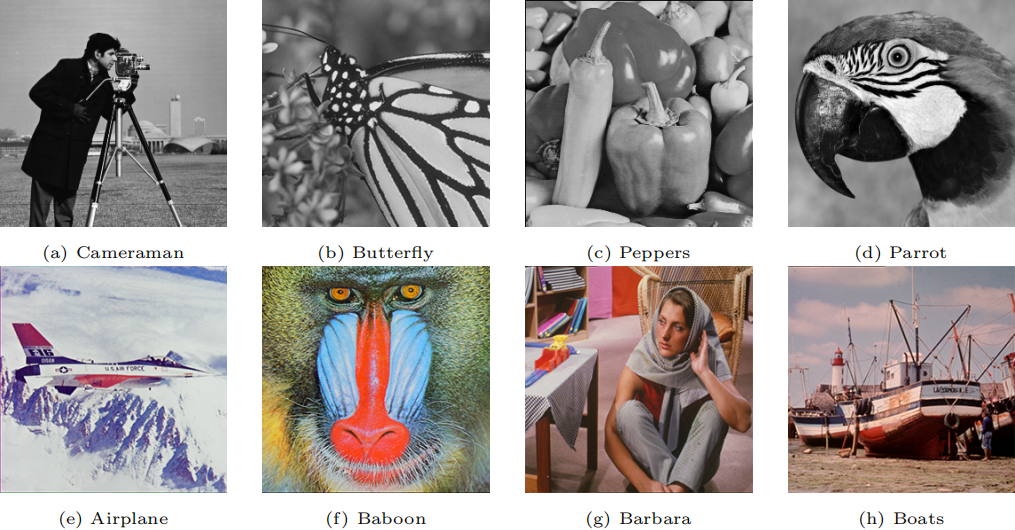
Figure 1: Test images.

The regularization parameter $\tau$, which regulates how much filtering is introduced by the regularization, has a significant impact on the model restoration’s effectiveness. In order to enable the model to sufficiently filter out noise while retaining as much of the original image information as possible, we hope to determine a suitable parameter value. The regularization parameters for TV and ATV are chosen based on experience. We are still using the regularization parameters from [14] here. We select the same regularization parameter settings for STV and WSTV to make it easier to compare the experimental findings. Additionally, debugging is used to determine the regularization parameters for the VTV model in the color experiment. The size of the Gaussian convolutional kernel $K$ is $3\times 3$ with a standard deviation of $\sigma=0.5$, which is applicable to STV and WSTV.

The test images used for grayscale image denoising are taken from Figure 1, including Cameraman, Butterfly, Peppers, and Parrot. The cameraman is primarily made up of smooth elements, whereas the butterfly has more edges and the parrot has more textures. Therefore, using these images to assess our suggested model is appropriate. By introducing Gaussian noise with standard deviations of 0.01, 0.05, and 0.1, respectively, we produce test data. Table 1 demonstrates that the four models all exhibit strong recovery effects at low noise levels $(\sigma=0.05)$. Consider the image butterfly as an example; their PSNR and SSIM differ only slightly. This is a result of the TV model’s ability to maintain crisp edges. However, as seen in Table 1 of these four sets of images, when the Gaussian noise is set to 0.1, our suggested model beats existing TV-based denoising models and the STV model in terms of PSNR and SSIM. Our model can keep more image details throughout the processing of image denoising.

Noise	0.01			0.05			0.10
Image	Cameraman
Models	$\lambda$	PSNR	SSIM	$\lambda$	PSNR	SSIM	$\lambda$	PSNR	SSIM
TV	15.00	29.2500	0.8378	6.30	25.7506	0.7774	4.70	24.6286	0.7535
ATV	12.30	30.0841	0.8384	4.00	26.6814	0.7782	2.70	25.5190	0.7567
STV	0.03	31.2149	0.8723	0.05	28.7940	0.8319	0.08	26.7526	0.7961
WSTV	0.03	31.5218	0.8759	0.05	29.1260	0.8369	0.08	27.1197	0.8031
Image	Butterfly
Models	$\lambda$	PSNR	SSIM	$\lambda$	PSNR	SSIM	$\lambda$	PSNR	SSIM
TV	21.90	32.3094	0.9375	11.40	28.7162	0.8870	8.90	26.9484	0.8524
ATV	17.30	32.9043	0.9354	7.00	28.4872	0.8693	5.30	27.0011	0.8414
STV	0.03	32.5432	0.9412	0.05	29.4395	0.9045	0.08	26.9123	0.8583
WSTV	0.03	32.8162	0.9428	0.05	29.7098	0.9078	0.08	27.1812	0.8633
Image	Peppers
Models	$\lambda$	PSNR	SSIM	$\lambda$	PSNR	SSIM	$\lambda$	PSNR	SSIM
TV	13.70	24.7045	0.8558	6.10	23.6823	0.7937	4.70	23.2066	0.7668
ATV	11.40	31.6726	0.8904	5.10	28.1475	0.8300	4.10	27.1115	0.8042
STV	0.03	33.3214	0.9158	0.05	30.5813	0.8815	0.08	28.1892	0.8388
WSTV	0.03	33.5545	0.9174	0.05	30.8369	0.8845	0.08	28.4602	0.8431
Image	Parrot
Models	$\lambda$	PSNR	SSIM	$\lambda$	PSNR	SSIM	$\lambda$	PSNR	SSIM
TV	21.10	31.2413	0.8899	9.50	27.5579	0.8283	7.30	26.2005	0.8012
ATV	17.20	31.6886	0.8861	6.30	27.9682	0.8174	5.90	27.2882	0.8090
STV	0.03	31.6012	0.8934	0.05	29.0395	0.8545	0.08	26.8955	0.8150
WSTV	0.03	31.8802	0.8958	0.05	29.3278	0.8585	0.08	27.2022	0.8204

Table 1: Compare the PSNR and SSIM of different models in grayscale image denoising.

We specifically carry out denoising studies with two example images, a cameraman and a butterfly, at a noise level of 0.05. To more easily see the denoising impact of each model, we will locally magnify the denoising image and incorporate it into Figure 2. First, for the cameraman, we notice that the borders restored by the TV model are quite hazy, the ATV model creates significant stepped artifacts, and the STV model and WSTV model work well. In butterfly, we find that WSTV can preserve more image details than the other three models, such as a shallow vertical line in the middle of the image. Figure 3 shows that the TV has the fastest denoising speed, followed by the ATV, in terms of each denoising model’s running duration. This is due to the ease with which TV and ATV can be numerically solved. It is inevitable that our methodology will be somewhat slower than the TV-based denoising models due to the complexity of operators in STV and WSTV. Consequently, in our next stage of development, a succinct and efficient algorithm will be taken into account.

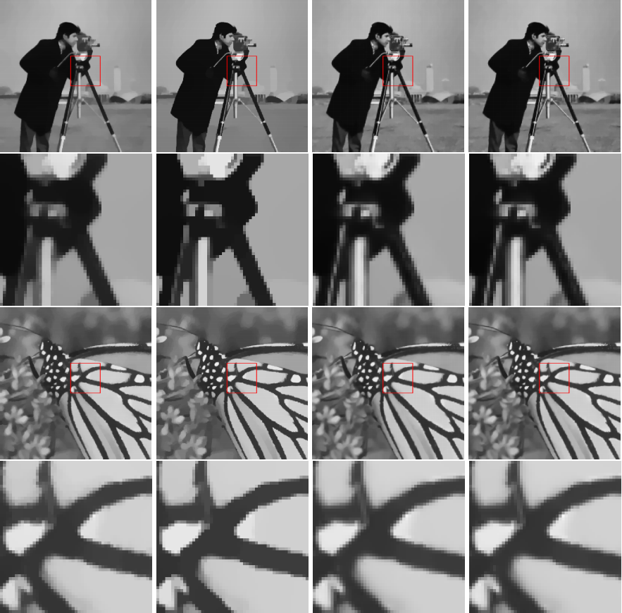
Figure 2: Compare the grayscale image denoising effects of various models at a noise level of 0.05. The first line of each image represents the complete restored image. The second line of each image is a portion of the restored image.

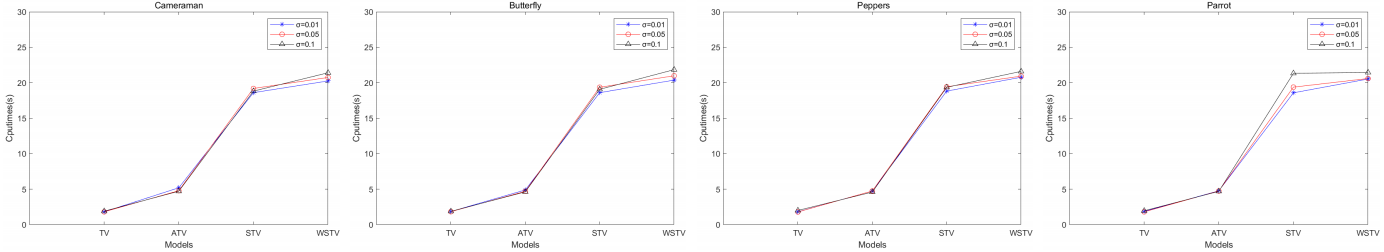
Figure 3: Compare the running time of different models in grayscale image denoising.

The test images used for color image denoising are taken from Figure 1, including Airplane, Baboon, Barbara, and Boats. For comparison purposes during the experiment, we employ the vector-extended VTV [19] of the TV model. Table 2 demonstrates that at three distinct noise levels, WSTV provides a higher PSNR or SSIM than STV and VTV. This also implies that our proposed model is more robust than other models when restoring degraded images. Figure 4 shows the denoising effects of three denoising models at noise levels of 0.05 and 0.1, respectively. This can further demonstrate that our model is superior in color image denoising. Additionally, we discover that the STV model and WSTV model outperform the VTV model in the experimental phase by achieving convergence with fewer iterations. Our model runs longer than STV and VTV because of the inclusion of convolutional kernels and the complexity of the operators.

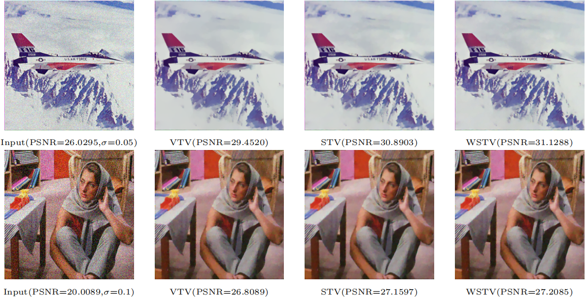
Figure 4: Compare the denoising effects of three denoising models at noise levels of 0.05 and 0.1.

Noise	0.01			0.05			0.10
Image	Airplane
Models	$\lambda$	PSNR	SSIM	$\lambda$	PSNR	SSIM	$\lambda$	PSNR	SSIM
VTV	21.3	33.4033	0.9506	10.5	29.4520	0.9142	9.3	27.8259	0.8558
STV	0.03	34.2178	0.9535	0.05	30.8903	0.9289	0.08	28.0012	0.8696
WSTV	0.03	34.4964	0.9545	0.05	31.1288	0.9306	0.08	28.0399	0.8581
Image	Baboon
Models	$\lambda$	PSNR	SSIM	$\lambda$	PSNR	SSIM	$\lambda$	PSNR	SSIM
VTV	22.1	28.9496	0.9443	13.7	25.8320	0.8901	11.1	24.0874	0.8523
STV	0.03	29.5672	0.9517	0.05	26.1500	0.8975	0.08	23.7505	0.8296
WSTV	0.03	29.9485	0.9554	0.05	26.4748	0.9053	0.08	24.0007	0.8421
Image	Babara
Models	$\lambda$	PSNR	SSIM	$\lambda$	PSNR	SSIM	$\lambda$	PSNR	SSIM
VTV	24.2	32.8200	0.9571	14.2	29.4384	0.9288	9.4	26.8089	0.8876
STV	0.03	32.8332	0.9551	0.05	29.7878	0.9310	0.08	27.1597	0.8935
WSTV	0.03	33.0999	0.9566	0.05	30.0102	0.9335	0.08	27.2085	0.8936
Image	Boats
Models	$\lambda$	PSNR	SSIM	$\lambda$	PSNR	SSIM	$\lambda$	PSNR	SSIM
VTV	23.8	33.1730	0.9662	14.2	29.7672	0.9375	10.6	26.9883	0.8675
STV	0.03	33.4654	0.9671	0.05	30.0880	0.9411	0.08	27.2988	0.8937
WSTV	0.03	33.7300	0.9682	0.05	30.3107	0.9432	0.08	27.3665	0.8899

Table 2: Compare the PSNR and SSIM of different models in color image denoising.

6 Conclusion

In this paper, we propose a novel image denoising model based on weighted structure tensor total variation (WSTV). The weighted matrix constructed by the edge indicator function is coupled to the gradient operator to describe the local features, and it is applied to the STV so that more details of the image can be saved. At the same time, the FISTA algorithm is used to accelerate the GP method, which greatly improves the convergence rate. The experimental results demonstrate that the denoising performance of the model is improved compared with the other TV-based denoising models and STV. Additionally, whether it is possible to create such an accelerated algorithm to increase the algorithm’s efficiency and decrease the running time is a related research subject.

References

- [1] R. C. Gonzalez, Digital image processing, Pearson education india (2009).
- [2] Z.-F. Pang, G. Meng, H. Li, et al., “Image restoration via the adaptive tvp regularization,”Computers and Mathematics with Applications. 80(5), 569-587 (2020).
- [3] A. Danielyan, V. Katkovnik, and K. Egiazarian, “BM3D Frames and Variational Image Deblurring,” IEEE Transactions on Image Processing. 21(4), 1715-1728 (2012).
- [4] J. Wu, X. Wang, X. Mou, et al., “Low dose ct image reconstruction based on structure ten-sor total variation using accelerated fast iterative shrinkage thresholding algorithm,” Sensors. 20(6), 1647 (2020).
- [5] Sung, Cheol, Park, et al., “Super-resolution image reconstruction: a technical overview,” IEEE Signal Processing Magazine. 20(3), 21-36 (2003).
- [6] L. I. Rudin, S. Osher, and E. Fatemi, “Nonlinear total variation based noise removal algo-rithms,” Physica D: Nonlinear Phenomena. 60(1-4), 259-268 (1992).
- [7] C.R. Vogel, Computational methods for inverse problems, SIAM (2002).
- [8] D. Strong and T. Chan, “Edge-preserving and scale-dependent properties of total variation regularization,” IEEE Inverse problems. 19(6), S165 (2003).
- [9] M. Lysaker, A. Lundervold, and X.-C. Tai, “Noise removal using fourth-order partial differential equation with applications to medical magnetic resonance images in space and time,” IEEE Transactions on Image Processing. 12(12), 1579-1590 (2003).
- [10] I. Chan, A. Marquina, and P. Mulet, “High-order total variation-based image restoration,” SIAM Journal on Scientific Computing. 22(2), 503-516 (2000).
- [11] K. Bredies, K. Kunisch, and T. Pock, “Total generalized variation,” SIAM Journal on lmaging Sciences. 3(3), 492-526 (2010).
- [12] F. Knoll, K. Bredies, T. Pock, et al., “Second order total generalized variation (tgv) for mri,” Magnetic Resonance in Medicine. 65(2), 480-491 (2011).
- [13] Bayram and M. E. Kamasak, “Directional total variation,” IEEE Signal Processing Letters. 19(12), 781-784 (2012).
- [14] Z.-F. Pang, Y.-M. Zhou, T. Wu, et al., “Image denoising via a new anisotropic total-variation-based model,” Signal Processing: Image Communication. 74, 140-152 (2019).
- [15] G. Gilboa and S. Osher, “Nonlocal operators with applications to image processing,” Multi-scale Modeling and Simulation. 7(3), 1005-1028 (2009).
- [16] M. Grasmair and F. Lenzen, “Anisotropic total variation filtering,” Applied Mathematics And Optimization. 62(3), 323-339 (2010).
- [17] J. Weickert et al., Anisotropic diffusion in image processing, vol. 1, Teubner Stuttgart (1998)
- [18] S. Lefkimmiatis A. Roussos, P Maragos, et al., “Structure tensor total variation,” SIAM Journal on Imaging Sciences. 8(2), 1090-1122 (2015).
- [19] X. Bresson and T. F. Chan, “Fast dual minimization of the vectorial total variation norm and applications to color image processing,” Inverse problems and imaging. 2(4), 455-484 (2008).
- [20] S. Lefkimmiatis, J. P. Ward, and M. Unser, “Hessian schatten-norm regularization for linear inverse problems,” IEEE Transactions on Image Processing. 22(5), 1873-1888 (2013).
- [21] A. Beck and M. Teboulle, “Fast gradient-based algorithms for constrained total variation image denoising and deblurring problems,” IEEE Transactions on Image Processing. 18(11), 2419-2434 (2009).
- [22] S. Lefkimmiatis and S. Osher, “Nonlocal structure tensor functionals for image regularization,” IEEE Transactions on Computational Imaging. 1(1), 16-29 (2015).
- [23] Sra, Suvrit, “Fast projections onto -norm balls for grouped feature selection,” Machine Learning and Knowledge Discovery in Databases: European Conference, ECML PKDD 2011, Athens, Greece, September 5-9, 2011, Proceedings, Part III 22, 305–317 (2011).