Knotted surfaces constructed using generators of the BMW algebras and their graphical description

Abstract.

We consider knotted surfaces and their graphical description that include 2-dimensional braids and their chart description. We introduce a new construction of surfaces in $D^{2}\times I\times I$, called BMW surfaces, that are described as the trace of deformations of tangles generated by generators $g_{i},g_{i}^{-1},e_{i}$ of the BMW (Birman-Murakami-Wenzl) algebras, where $g_{i}$ and $g_{i}^{-1}$ are a standard generator of the $n$-braid group and its inverse, and $e_{i}$ is a tangle consisting of a pair of “hooks”. And we introduce a notion of BMW charts that are graphs in $I\times I$ and show that a BMW surface has a BMW chart description.

1. Introduction

In this paper, we treat tangles and surfaces that are locally flatly and properly embedded. Let $I=[0,1]$, and let $n$ be a positive integer. A 2-dimensional braid, also called a simple surface braid, or a simple braided surface [2, 3] of degree $n$ is a surface $S$ properly embedded in $D^{2}\times I_{3}\times I_{4}$, where $I_{3}=I_{4}=I$, such that $S\cap(D^{2}\times\{t\})$ consists of $n$ or $n-1$ points for any $t\in I_{3}\times I_{4}$. A 2-dimensional braid can be regarded as the trace of deformations of braids in $D^{2}\times I_{3}$, where each deformation is either by isotopies of braids or application of band surgery, that can be presented by deformation of braid words by braid relations or by an addition/deletion of a letter. A 2-dimensional braid is described by a finite graph called a “chart” in $I_{3}\times I_{4}$, that describes the deformation of braid words.

In this paper, we consider knotted surfaces and their graphical description that include 2-dimensional braids and their chart description. We introduce a new construction of surfaces in $D^{2}\times I_{3}\times I_{4}$, called “BMW surfaces”, that are described as the trace of deformations of tangles called BMW tangles that are generated by generators of the BMW (Birman-Murakami-Wenzl) algebras [1, 10, 11]. The BMW algebra of degree $n$ has two types of generators $g_{i},g_{i}^{-1}$ and $e_{i}$, where $g_{i}$ and $g_{i}^{-1}$ are a standard generator of the $n$-braid group and its inverse, and the additional generator $e_{i}$ is a pair of “hooks” between the $i$th and $(i+1)$th boundary points of the tangle as shown in Fig. 1. And we introduce the notion of a graphical description called “BMW charts” that present BMW surfaces.

The paper is organized as follows. In Section 2, we give definition of BMW tangles, and in Section 3, we treat two types of equivalence relation for BMW tangles: regular isotopy and BMW tangle isotopy. In Section 4, we review the motion picture method by which we describe BMW surfaces. In Section 5, we give regular BMW surfaces and BMW surfaces, and (regular) BMW charts. A (regular) BMW surface is presented by a (regular) BMW chart (Theorem 5.6). In Section 6, we show Theorem 5.6. In Section 7, we give local moves of BMW charts called BMW chart moves. In Section 8, we introduce additional types of vertices of BMW charts. We close the paper with further questions in Section 9. We give [2, 3, 9] for basics of 1-dimensional and 2-dimensional knot theory.

2. BMW tangles

In this section, we give the definition of a BMW tangle. A BMW tangle of degree $n$ is called an $n$-knit in [11]. A BMW tangle is generated by generators of the BMW algebra [1, 10, 11], the traces of whose irreducible representations are related to the Kauffman 2-variable polynomial; the BMW algebra is considered as an analogue of the Iwahori-Hecke algebra that is related to the Jones polynomial.

Let $n$ be a positive integer. Let $I=I_{1}=I_{2}=[0,1]$ and $D^{2}=I_{1}\times I_{2}$. A tangle in $D^{2}\times I$ is a set of intervals and circles properly embedded in $D^{2}\times I$. Let $p_{i}=i/(n+1)$ and $q_{i}=(1/2,p_{i})$ $(i=1,2,\ldots,n)$, and let $Q_{n}=\{q_{1},q_{2},\ldots,q_{n}\}$, a set of $n$ interior points of $D^{2}$. Let $\mathbf{1}=Q_{n}\times I$, the representative of the trivial $n$-braid in the cylinder $D^{2}\times I$ with the starting point set $Q_{n}$.

Let $g_{i}$ $(i=1,\ldots,n-1)$ be the representative of a standard generator of the $n$-braid group in the cylinder $D^{2}\times I$, that is, $g_{i}$ is the set of $n$ intervals properly embedded in $D^{2}\times I$ such that the diagram of $g_{i}$ is as in the left figure of Fig. 1; more precisely, $g_{i}$ is the set of $n$ embedded intervals such that $g_{i}\cap I_{1}\times([0,p_{i}-\delta]\cup[p_{i+1}+\delta,1])\times I=\{q_{1},\ldots,q_{n-1},q_{n+2},\ldots,q_{n}\}\times I$, where $\delta=1/(2(n+1))$, and $g_{i}\cap I_{1}\times[p_{i}-\delta,p_{i+1}+\delta]\times I=\cup_{u\in[0,1]}\phi_{u}(\{q_{i},q_{i+1}\})\times\{u\}$, where we consider the circle $S^{1}$ containing $q_{i}$ and $q_{i+1}$ as antipodal points, and $\{\phi_{u}:S^{1}\to S^{1}\}_{u\in[0,1]}$ is a homotopy between the identity map and the rotation by $\pi$ around the center $(q_{i}+q_{i+1})/2$ such that each $\phi_{u}$ is a rotation by $\pi u$. Let $g_{i}^{-1}$ be the inverse of $g_{i}$, that is as in the middle figure of Fig. 1; more precisely, $g_{i}^{-1}$ is the same with $g_{i}$ except that $g_{i}\cap I_{1}\times[p_{i}-\delta,p_{i+1}+\delta]\times I=\cup_{u\in[0,1]}\phi_{1-u}(\{q_{i},q_{i+1}\})\times\{u\}$.

Let $e_{i}$ $(i=1,\ldots,n-1)$ be the set of $n+1$ intervals properly embedded in $D^{2}\times I$ such that $e_{i}\cap I_{1}\times([0,p_{i}-\delta]\cup[p_{i+1}+\delta,1])\times I=\{q_{1},\ldots,q_{n-1},q_{n+2},\ldots,q_{n}\}\times I$, where $\delta=1/(2(n+1))$, and $e_{i}\cap I_{1}\times[p_{i}-\delta,p_{i+1}+\delta]\times I$ consists of a pair of semicircles in $\{1/2\}\times[p_{i}-\delta,p_{i+1}+\delta]\times I$ such that one connects $(q_{i},0)$ and $(q_{i+1},0)$ with the center $(q_{i}+q_{i+1})/2,0)$ and the other connects $(q_{i},1)$ and $(q_{i+1},1)$ with the center $(q_{i}+q_{i+1})/2,1)$. We call an arc of $e_{i}$ a hook. The diagram of $e_{i}$ is as in the right figure of Fig. 1.

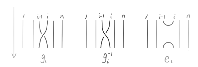
Figure 1. The generators $g_{i}$, $g_{i}^{-1}$ and $e_{i}$.

For $w,w^{\prime}\in\{g_{i},g_{i}^{-1},e_{i}\mid i=1,2,\ldots,n-1\}$, we define the product $w\cdot w^{\prime}$ as follows. Let $f_{1}:D^{2}\times I\to D^{2}\times[0,1/2]$, $f_{1}(x,t)=(x,t/2)$, and $f_{2}:D^{2}\times I\to D^{2}\times[1/2,1]$, $f_{2}(x,t)=(x,(t+1)/2)$. Then we define $w\cdot w^{\prime}=f_{1}(w)\cup f_{2}(w^{\prime})$; see Fig. 2, and we denote $w\cdot w^{\prime}$ by $ww^{\prime}$.

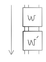
Figure 2. The product $w\cdot w^{\prime}$.

Let $F_{n}$ be the set consisting of $\mathbf{1}$ and products of a finite number of elements of $\{g_{i},g_{i}^{-1},e_{i}\mid i=1,2,\ldots,n-1\}$, where each product is in the form of $(\cdots((w_{1}w_{2})w_{3})\cdots w_{m-1})w_{m}$ for some $m$, where $w_{1},\ldots,w_{m}\in\{g_{i},g_{i}^{-1},e_{i}\mid i=1,2,\ldots,n-1\}$. We denote $(\cdots((w_{1}w_{2})w_{3})\cdots w_{m-1})w_{m}$ by $w_{1}w_{2}w_{3}\cdots w_{m}$. We call an element of $F_{n}$ a word, and we call each element of $\{g_{i},g_{i}^{-1},e_{i}\mid i=1,2,\ldots,n-1\}$ forming a word a letter.

We consider an equivalence relation for tangles in $D^{2}\times I$ that are related by isotopies defined as follows; so that the set of equivalence classes has one-to-one correspondence with $F_{n}$. We remark that concerning the ambient isotopy of Definition 2.1, that of (1) does not change the diagram of the tangle, and because of the ambient isotopy of (2) the associative law for products holds true, and that of (3) changes the minimal/maximal point of a hook (with respect to the $I$ direction) to an interval. For the case of a braid in $D^{2}\times I$, the order of letters of its braid word presentation is determined by $I$ coordinates of crossings. For a BMW tangle, we determine that the order of letters is determined by $I$ coordinates of crossings and hooks, where the $I$ coordinate of each $e_{i}$ is determined as the middle point of $I$ coordinates of the maximal point and the minimal point of $e_{i}$: for example, the lower right figure of Fig. 3 is presented by $e_{1}e_{3}$; so we consider the ambient isotopy of (4). We remark that the ambient isotopy of (3) is included in that of (4), but we write it to claim that it is a defomration of one hook. We also remark that the condition in (2) is required so that we determine the “position” of circle components: for example, to distinguish $e_{1}e_{1}e_{3}$ and $e_{1}e_{3}e_{3}$.

For a tangle $\tau$ in $D^{2}\times I$, an upper hook (resp. lower hook) of $\tau$ is an arc of $\tau$ in $I_{1}\times I_{2}^{\prime}\times[t_{0},t_{1}]$ for some intervals $I_{2}^{\prime}\subset I_{2}$ and $[t_{0},t_{1}]\subset I$, satisfying the following, where $p:I_{1}\times I_{2}^{\prime}\times\{t\}\to I_{2}^{\prime}$ is the projection.

1. At $t=t_{1/2}=(t_{0}+t_{1})/2$, $\tau\cap(I_{1}\times I_{2}^{\prime}\times\{t\})$ consists of a point or an arc $c$ such that $p(c)$ is an interval homeomorphic to $c$ by $p$.

2. For $t\in[t_{0},t_{1/2})$ (resp. $(t_{1/2},t_{1}]$), $\tau\cap(I_{1}\times I_{2}^{\prime}\times\{t\})$ consists of a pair of points $x$ and $x^{\prime}$ such that $p(x)\neq p(x^{\prime})$.

3. For $t\in(t_{1/2},t_{1}]$ (resp. $[t_{0},t_{1/2})$), $\tau\cap(I_{1}\times I_{2}^{\prime}\times\{t\})=\emptyset$.

We call a point of $\tau\cap(I_{1}\times I_{2}^{\prime}\times\{t_{1/2}\})$ a minimal point (resp. maximal point); remark that in the case when $\tau\cap(I_{1}\times I_{2}^{\prime}\times\{t_{1/2}\})$ consists of a point, it is uniquely determined. We call an upper/lower hook simply a hook. A pair of hooks is a pair of arcs of $\tau$ in some $I_{1}\times I_{2}^{\prime}\times[t_{0},t_{1}]$ such that $\tau\cap(I_{1}\times I_{2}^{\prime}\times[t_{0},t_{1/2}])$ is an upper hook and $\tau\cap(I_{1}\times I_{2}^{\prime}\times[t_{1/2},t_{1}])$ is a lower hook, and we call $I_{1}\times I_{2}^{\prime}\times I^{\prime}$ a regular neighborhood of the pair of hooks. We say that two regular neighborhoods are the same if they contain the same set of minimal and maximal points of hooks.

Definition 2.1.

Let $\tilde{\tau}$ be a tangle, that is a set of intervals and circles properly embedded in $D^{2}\times I$, such that hooks are in the form of pairs of hooks and their regular neighborhoods are uniquely determined. Then, $\tilde{\tau}$ is equivalent to an element $w$ of the set $F_{n}$, if $\tilde{\tau}$ is carried to $w$ by a finite sequence of ambient isotopies of $D^{2}\times I$, where each ambient isotopy $\{f_{u}\}_{u\in[0,1]}$ is one of the following. Let $\tau$ and $\tau^{\prime}$ be tangles related by $\{f_{u}\}_{u\in[0,1]}$ with $f_{0}(\tau)=\tau$ and $f_{1}(\tau)=\tau^{\prime}$.

1. For each $u$, $f_{u}=h_{u}\times\mathrm{id}_{I_{2}\times I}$ for an ambient isotopy $\{h_{u}\}_{u\in[0,1]}$ of $I_{1}$.

2. For each $u$, $f_{u}=\mathrm{id}_{I_{1}}\times h_{u}$ for a fiber-preserving ambient isotopy $\{h_{u}\}_{u\in[0,1]}$ of $I_{2}\times I$, where fiber is $I_{2}\times\{t\}$ $(t\in I)$, satisfying the following. For any pair of hooks, let $I_{1}\times I_{2}^{\prime}\times I^{\prime}$ be its regular neighborhood. Then, for any pair of hooks, $h_{u}(I_{2}^{\prime}\times I^{\prime})=I_{2,u}^{\prime}\times I^{\prime}_{u}$ for intervals $I_{2,u}^{\prime}\subset I_{2}$ and $I^{\prime}_{u}\subset I^{\prime}$ $(u\in[0,1])$.

3. For each $u$, $f_{u}$ is an ambient isotopy of $I_{1}\times I_{2}\times I$ relative to the complement of a 3-disk $I_{1}\times I_{2}^{\prime}\times I^{\prime}$, where $I_{2}^{\prime}\subset I_{2}$ and $I^{\prime}\subset I$, given as follows. We require the following situation: $\tau\cap(I_{1}\times I_{2}^{\prime}\times I^{\prime})$ is a hook. Then $f_{u}$ is an ambient isotopy such that for any $u\in[0,1]$, $f_{u}(\tau\cap(I_{1}\times I_{2}^{\prime}\times I^{\prime}))$ is a hook; see Fig. 3.

4. For each $u$, $f_{u}$ is an ambient isotopy of $I_{1}\times I_{2}\times I$ relative to the complement of a 3-disk $I_{1}\times I_{2}^{\prime}\times I^{\prime}$, where $I_{2}^{\prime}\subset I_{2}$ and $I^{\prime}\subset I$, given as follows. We require the following situation: $\tau\cap(I_{1}\times I_{2}^{\prime}\times I^{\prime})$ is a pair of hooks. Then, $f_{u}$ is defined as follows. Let $x_{0}$ and $x_{1}$ be minimal and maximal points of the pair of hooks, and let $t_{0}$ and $t_{1}$ be the $I^{\prime}$ coordinates of $x_{0}$ and $x_{1}$. Put $t_{1/2}=(t_{0}+t_{1})/2$. Then, $f_{u}$ is an ambient isotopy such that $f_{u}(\tau\cap(I_{1}\times I_{2}^{\prime}\times I^{\prime}))$ is a pair of hooks, and $t_{0,u}$ and $t_{1,u}$, that are the $I^{\prime}$ coordinates of $f_{u}(x_{0})$ and $f_{u}(x_{1})$, satisfy $(t_{0,u}+t_{1,u})/2=t_{1/2}$ for any $u\in[0,1]$; see Fig. 3.

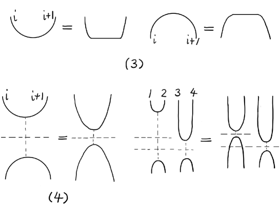
Figure 3. Equivalence of (3) and (4), here we omit the $j$th strings for $j\neq i,i+1$. By (4), the lower right figure is presented by $e_{1}e_{3}$.

From now on, we consider the equivalence classes and we denote them using the same notations $\mathbf{1},g_{i},g_{i}^{-1}$ and $e_{i}$.

By definition, the set of equivalence classes of $F_{n}$ forms a free semi-group with identity element $\mathbf{1}$ generated by $\{g_{i},g_{i}^{-1},e_{i}\mid i=1,2,\ldots,n-1\}$, and we call each element (or its representative) a BMW tangle of degree $n$. Since the association law holds true, we omit parentheses for products of BMW tangles. Remark that a BMW tangle is presented by a unique word $\mathbf{1}$ or $w_{1}w_{2}\cdots w_{m}$ for some $m$, where $w_{1},\ldots,w_{m}\in\{g_{i},g_{i}^{-1},e_{i}\mid i=1,2,\ldots,n-1\}$.

We formulate the definition of a BMW tangle as follow.

Definition 2.2.

Let $\tau$ be a tangle, that is a set of a finite number of intervals and circles embedded properly in $D^{2}\times I$, such that hooks are in the form of pairs of hooks and their regular neighborhoods are uniquely determined. Then $\tau$ is called a BMW tangle of degree $n$ if it is presented by a word $w_{1}w_{2}\cdots w_{m}$, where $w_{j}\in\{g_{i},g_{i}^{-1},e_{i}\mid i=1,2,\ldots,n-1\}\subset F_{n}$ and the equivalence is given in Definition 2.1. For a BMW tangle $\tau$, $\tau\cap\partial(D^{2}\times I)=Q_{n}\times\{0,1\}$, where $Q_{n}$ is a set of $n$ interior points of $D^{2}$. We call an element of $Q_{n}\times\{0,1\}$ a boundary point of $\tau$.

3. Regular isotopy and BMW tangle isotopy of BMW tangles

In this section, we give two types of equivalence relation for BMW tangles: regular isotopy [8] and BMW tangle isotopy.

For a tangle $\tau$ in $D^{2}\times I$, the projection $p:D^{2}\times I\to I_{2}\times I$ is regular if the singularities consists of a finite number of transverse double points, called crossings. For $\tau$ such that $p:D^{2}\times I\to I_{2}\times I$ is a regular projection, the diagram of $\tau$ is the projected image $p(\tau)$ in $I_{2}\times I$ such that we equip each crossing with over/under information with respect to the $I_{1}$ direction, by erasing a small segment of the under arc around the crossing.

By definition of BMW tangles, we have the following.

Lemma 3.1.

Two BMW tangles are the same if their diagrams are related by an ambient isotopy of $I_{2}\times I$.

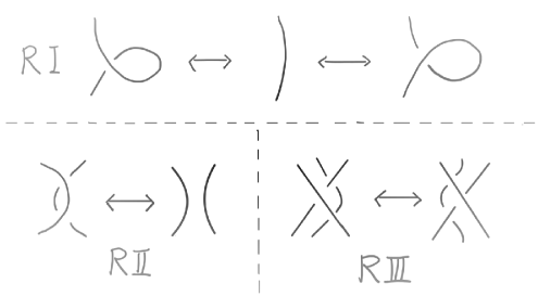
Figure 4. Reidemeister moves of types I, II and III, denoted by RI, RII, and RIII, respectively.

Reidemeister moves of types I, II and III are local moves for diagrams as depicted in Fig. 4.

We say that two BMW tangles $\tau$ and $\tau^{\prime}$ of degree $n$ are regular isotopic if they are related by a finite sequence of ambient isotopies of $D^{2}\times I$ such that each ambient isotopy $\{f_{u}\}_{u\in[0,1]}$ is fiber-preserving, where fiber is $\{t\}\times I_{2}\times I$ $(t\in I_{1})$, or $\{f_{u}\}_{u\in[0,1]}$ is an ambient isotopy that defines equivalence of BMW tangles in Definition 2.1. We call the ambient isotopy relating regular isotopic $\tau$ and $\tau^{\prime}$ a regular ambient isotopy. By definition, we have the following.

Lemma 3.2.

Two BMW tangles of degree $n$ are regular isotopic if and only if their diagrams are related by a finite sequence of Reidemeister moves of types II and III, and ambient isotopies of $I_{2}\times I$.

Proof.

First we discuss that Reidemeister moves of types II and III are realized by regular isotopies. For a tangle $\tau$ in $D^{2}\times I$ such that the projection $p:D^{2}\times I\to I_{2}\times I$ is regular, in the following argument, deformation of $\tau$ is deformation by an ambient isotopy of $D^{2}\times I$ that defines equivalence of BMW tangles in Definition 2.1. We apply a Reidemeister move to the diagram of $\tau$. For $\tau$ in $D^{2}\times I$ and its diagram in $I_{2}\times I$, we can deform $\tau$ so that the diagram is unchanged and one arc (resp. two arcs) concerning a Reidemeister move of type II (resp. type III) are unmoved and the other arc is in a 2-disk before and after the Reidemeister move. Further, we can deform $\tau$ so that the 2-disk is in $\{1/2\}\times I_{2}\times I$. Hence, these types of Reidemeister moves are realized by regular ambient isotopies. Therefore the if part holds true.

However, in the above situation, when we apply a Reidemeister move of type I, we cannot deform $\tau$ so that the arc of $\tau$ concerning the Reidemeister move is in a 2-disk, since there is a self-crossing. Hence Reidemeister moves of type I cannot be realized by regular ambient isotopies. Since an ambient isotopy of $D^{2}\times I$ relates $\tau$ and $\tau^{\prime}$ if and only if their diagrams are related by a finite sequence of Reidemeister moves of types I, II and III, and ambient isotopies of $I_{2}\times I$, the only if part holds true. ∎

Let $E\times I^{\prime}$ be a cylinder, where $E$ is a 2-disk and $I^{\prime}$ is an interval. For a BMW tangle $\tau$, we define an ambient isotopy of $D^{2}\times I$ presenting a rotation of the 2-disk $E$ in a cylinder $E\times I^{\prime}$, as follows. First, we require that $E$ is contained in $D^{2}$ and $I^{\prime}$ is contained in $I$ such that $\tau\cap\partial(E\times I^{\prime})$ consists of a finite number of transverse intersection points of arcs of $\tau$ and $E\times\partial I^{\prime}$.

We identify $E$ with the unit disk $\{z\mid|z|\leq 1\}\subset\mathbb{C}$ and we identify $I^{\prime}$ with $[0,1]$. Let $\{h_{u}\}_{u\in[0,1]}$ be an ambient isotopy of $E$ defined by $h_{u}(z)=ze^{iu\theta}$ for some $\theta\in\mathbb{R}\backslash\{0\}$. Then construct an ambient isotopy $\{f_{u}\}_{u\in[0,1]}$ of $E\times I^{\prime}$ by $f_{u}=h_{2u}(z)\times\mathrm{id}_{[0,1]}$ if $u\in[0,1/2]$ and $f_{u}=h_{2(1-u)}(z)\times\mathrm{id}_{[0,1]}$ if $u\in[1/2,1]$. Take a regular neighborhood $N(E)$ of $E$ in $D^{2}$ such that $\tau\cap(N(E)\backslash E)\times I^{\prime}=\emptyset$. Construct an ambient isotopy $\{\bar{f}_{u}\}_{u\in[0,1]}$ of $D^{2}\times I$ relative to the complement of $N(E)\times I^{\prime}$ such that $\bar{f}_{u}|_{E\times I^{\prime}}=f_{u}$. We call $\{\bar{f}_{u}\}_{u\in[0,1]}$ an ambient isotopy of $D^{2}\times I$ presenting a rotation by $\theta$ of the 2-disk $E$ in a cylinder $E\times I^{\prime}$.

We say that two BMW tangles $\tau$ and $\tau^{\prime}$ of degree $n$ are BMW tangle isotopic if they are related by a finite sequence of BMW tangles $\tau=\tau_{0},\tau_{1},\ldots,\tau_{m}=\tau^{\prime}$ such that $\tau_{j-1}$ and $\tau_{j}$ $(j=1,\ldots,m)$ are related by a regular ambient isotopy $\{f^{j}_{u}\}_{u\in[0,1]}$ or an ambient isotopy $\{f^{j}_{u}\}_{u\in[0,1]}$ presenting a rotation of a 2-disk $E_{j}$ in some cylinder $E_{j}\times I_{j}\subset D^{2}\times I$. For $\tau$ and $\tau^{\prime}$ that are BMW tangle isotopic, we call the ambient isotopy $\{f_{u}\}_{u\in[0,1]}$ relating $\tau$ and $\tau^{\prime}$ a BMW tangle ambient isotopy.

Lemma 3.3.

Two BMW tangles $\tau$ and $\tau^{\prime}$ of degree $n$ are BMW tangle isotopic if and only if their diagrams $\Gamma$ and $\Gamma^{\prime}$ are related by a finite sequence of diagrams $\Gamma=\Gamma_{0},\Gamma_{1},\ldots,\Gamma_{m}=\Gamma^{\prime}$ such that $\Gamma_{j-1}$ and $\Gamma_{j}$ are related by a Reidemeister move of type I presented by $e_{i}\leftrightarrow g_{i}^{\epsilon}e_{i}$ or $e_{i}\leftrightarrow e_{i}g_{i}^{\epsilon}$ $(\epsilon\in\{+1,-1\}$, $i\in\{1,2,\ldots,n-1\})$ (see Fig. 5), or a Reidemeiter move of type II, or type III or an ambient isotopy of $I_{2}\times I$, and moreover $\Gamma_{j-1}$ and $\Gamma_{j}$ present BMW tangles if they are related by a Reidemeister move of type I $(j=1,2,\ldots,m)$.

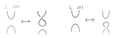
Figure 5. Reidemeister moves of type I presented by $e_{i}\leftrightarrow g_{i}e_{i}$ (left figure) or $e_{i}\leftrightarrow e_{i}g_{i}$ (right figure), $i\in\{1,2,\ldots,n-1\}$, where we omit the $j$th strings for $j\neq i-1,i$.

Proof.

Let $\tau$ and $\tau^{\prime}$ be BMW tangles such that $f_{0}(\tau)=\tau$ and $f_{1}(\tau)=\tau^{\prime}$ for an ambient isotopy $\{f_{u}\}_{u\in[0,1]}$ presenting a rotation of a 2-disk $E$ in a cylinder $E\times I^{\prime}\subset D^{2}\times I$. Since $\tau\cap\partial(E\times I^{\prime})$ consists of a finite number of transverse intersection points of arcs of $\tau$ and $E\times\partial I^{\prime}$, their diagrams are related by a finite sequence of Reidemeister moves of type I presented by $e_{i}\leftrightarrow g_{i}^{\epsilon}e_{i}$ or $e_{i}\leftrightarrow e_{i}g_{i}^{\epsilon}$ ($\epsilon\{+1,-1\}$, $i\in\{1,2,\ldots,n-1\}$), and Reidemeiter moves of types II and III and ambient isotopies of $I_{2}\times I$. Thus, together with Lemma 3.2, the only if part holds true.

For BMW tangles $\tau$ and $\tau^{\prime}$, if their diagrams are related by a Reidemeister move of type I presented by $e_{i}\leftrightarrow g_{i}^{\epsilon}e_{i}$ or $e_{i}\leftrightarrow e_{i}g_{i}^{\epsilon}$ $(\epsilon\in\{+1,-1\}$, $i\in\{1,2,\ldots,n-1\})$, then, for a cylinder $E\times I^{\prime}\subset D^{2}\times I$ containing the moving arc concerning the Reidemeister move, $\tau$ and $\tau^{\prime}$ are related by an ambient isotopy presenting a rotation by $\pm\pi$ of the 2-disk $E$ in $E\times I^{\prime}\subset D^{2}\times I$. And if diagrams are related by a Reidemeister move of type II or III, or an ambient isotopy of $I_{2}\times I$, then, by Lemma 3.2, $\tau$ and $\tau^{\prime}$ are regular isotopic. Thus the if part holds true. ∎

Let $\tau$ and $\tau^{\prime}$ be tangles in $D^{2}\times I$. Let $p:D^{2}\times I\to I_{2}\times I$ be the projection, and let $D=p(\tau)$ and $D^{\prime}=p(\tau^{\prime})$ be the diagrams of $\tau$ and $\tau^{\prime}$. Suppose that $D$ and $D^{\prime}$ are related by (1) a Reidemeister move or (2) an ambient isotopy of $I_{2}\times I$. Then, $\tau$ is carried to $\tau^{\prime}$ by an ambient isotopy $\{f_{u}\}_{u\in[0,1]}$ of $D^{2}\times I$ satisfying the conditions as follow.

1. If $D$ and $D^{\prime}$ are related by a Reidemeister move, then, for each $u\in[0,t)$ (resp. $u\in(t,1]$), where $t$ is a point of $\mathrm{Int}(I)$, $p(f_{u}(\tau))$ is related to $D$ (resp. $D^{\prime}$) by an ambient isotopy of $I_{2}\times I$.

2. If $D$ and $D^{\prime}$ are related by an ambient isotopy $\{h_{u}\}_{u\in[0,1]}$ of $I_{2}\times I$, then $p(f_{u}(\tau))=h_{u}(D)$ for any $u\in[0,1]$.

We call the ambient isotopy of (1) (resp. (2)) an ambient isotopy associated with a Reidemeister move (resp. an ambient isotopy of $I_{2}\times I$ relating the diagrams).

Claim 3.4.

Let $\tau$ and $\tau^{\prime}$ be BMW tangles of degree $n$ in $D^{2}\times I$ that are regular isotopic or BMW tangle isotopic. Let $D$ and $D^{\prime}$ be diagrams of $\tau$ and $\tau^{\prime}$, and let $D=D_{0}\to D_{1}\to\ldots\to D_{m}=D^{\prime}$ be a sequence of diagrams such that $D_{j-1}$ and $D_{j}$ $(j=1,\ldots,m)$ are related by a Reidemeister move or an ambient isotopy of $I_{2}\times I$. Let $\tau_{j}$ be a tangle whose diagram is $D_{j}$ $(j=1,\ldots,m-1)$. Then, $\tau$ and $\tau^{\prime}$ are related by a finite sequence of tangles $\tau=\tau_{0}\to\tau_{1}\to\ldots\to\tau_{m}=\tau^{\prime}$ such that $\tau_{j-1}$ and $\tau_{j}$ are related by an ambient isotopy $\{f_{u}^{j}\}_{u\in[0,1]}$ of $D^{2}\times I$ associated with a Reidemeister move or an ambient isotopy of $I_{2}\times I$ relating $D_{j-1}$ and $D_{j}$ $(j=1,\ldots,m)$.

From now on, we assume that a regular ambient isotopy or a BMW tangle ambient isotopy relating $\tau$ and $\tau^{\prime}$ is the ambient isotopy determined from these ambient isotopies $\{f_{u}^{j}\}_{u\in[0,1]}$ $(j=1,\ldots,m)$.

When we construct BMW surfaces in Section 5, we require that by each Reidemeister move or ambient isotopy of $I_{2}\times I$ for diagrams, a BMW tangle is carried to a BMW tangle. Moreover, we require that an ambient isotopy of $I_{2}\times I$ does not change the position of a circle component. So we give the following definition. For a diagram $D=p(\tau)$ of a tangle $\tau$, we call the image of a hook of $\tau$ by the projection $p$ a hook in $D$, and we call the image by $p$ of a boundary point of $\tau$ a boundary point of $D$.

Definition 3.5.

Let $\tau$ and $\tau^{\prime}$ be BMW tangles of degree $n$ such that their diagrams $D$ and $D^{\prime}$ are related by an ambient isotopy of $I_{2}\times I$. Let $\{h_{u}\}_{u\in[0,1]}$ be the ambient isotopy relating $D$ and $D^{\prime}$. Then, we say that $\{h_{u}\}_{u\in[0,1]}$ keeps the BMW tangle form if it is a composition of a finite sequence of ambient isotopies of $I_{2}\times I$ that relates a sequence of diagrams $D=D_{0}\to D_{1}\to\ldots,D_{m}=D^{\prime}$, satisfying the following:

1. The diagrams $D_{0},D_{1},\ldots,D_{m-1},D_{m}$ present BMW tangles of degree $n$.

2. Each ambient isotopy $\{h_{u}^{j}\}_{u\in[0,1]}$ relating $D_{j-1}$ and $D_{j}$ ($j=1,\ldots,m$) is relative to the complement of a disk $I_{2}^{\prime}\times I^{\prime}$ ($I_{2}^{\prime}\subset I_{2}$ and $I^{\prime}\subset I$) satisfying that $D^{\prime}_{j-1}=D_{j-1}\cap(I_{2}^{\prime}\times I^{\prime})$ is the diagram of a BMW tangle in $D^{2}\times I_{2}^{\prime}\times I^{\prime}$ such that each pair of hooks in $D_{j-1}^{\prime}$ is a pair of hooks in $D_{j-1}$, and moreover each component of $D_{j-1}^{\prime}$ is connected to a pair of boundary points in $\partial D_{j-1}^{\prime}=D_{j-1}^{\prime}\cap(I_{2}^{\prime}\times\partial I^{\prime})$.

In the situation of Claim 3.4, we say that BMW tangles $\tau$ and $\tau^{\prime}$ of degree $n$ are regular isotopic (resp. BMW tangle isotopic) by a regular ambient isotopy (resp. a BMW tangle ambient isotopy) keeping the BMW tangle form if $D=D_{0},D_{1},\ldots,D_{m-1},D_{m}=D^{\prime}$ are diagrams of BMW tangles of degree $n$, and each ambient isotopy of $I_{2}\times I$ relating the diagrams keeps the BMW tangle form.

4. Description of knotted surfaces

In this section, we review how to describe knotted surfaces as a “trace” of intersections with three-dimensional spaces [2, 3].

Let $S$ be a knotted surface properly embedded in $D^{2}\times I_{3}\times I_{4}$, and let $p:D^{2}\times I_{3}\times I_{4}\to I_{2}\times I_{3}\times I_{4}$ be the natural projection. By perturbing $S$ if necessary, we assume that $p$ is regular, that is, the singularities consists of a finite number of double point curves, isolated triple points and isolated branch points. The diagram of $S$ is the image $p(S)$ equipped with under/over information around each double point curve, that is obtained in such a way as follows. The diagram $p(S)$ consists of a finite number of disks, called sheets. Around each double point curve $c$, we call a sheet an over-sheet (resp. under-sheet) if the coordinate in the $I_{4}$ direction of the over-sheet is greater than that of the under-sheet, and we equip $p(S)$ with the over/under information by depicting the sheets around $c$ by one over-sheet and a pair of under-sheets.

We call the intersection $S\cap(D^{2}\times I_{3}\times\{t\})$ ($t\in I_{4}$) a slice of $S$ at $t$. We identify each slice with the image by the projection to $D^{2}\times I_{3}$. And when we have a tangle $\tau$ in $D^{2}\times I_{3}$ and an ambient isotopy $\{f_{t}\}_{t\in I^{\prime}}$ of $D^{2}\times I_{3}$, for some interval $I^{\prime}$, $\cup_{t\in I^{\prime}}f_{t}(\tau)\times\{t\}$ forms a properly embedded surface $S$ in $D^{2}\times I_{3}\times I^{\prime}$ such that the slice at $t$ is $f_{t}(\tau)$ ($t\in I^{\prime}$). We call the constructed surface $\cup_{t\in I^{\prime}}f_{t}(\tau)\times\{t\}$ the trace of $\tau$ by an ambient isotopy $\{f_{t}\}_{t\in I^{\prime}}$.

We also use the term “trace” for diagrams. The diagram of $S$ is described as the trace of diagrams of slices of $S$. When we describe $S$ by figures, we use the motion picture method, that is a sequence of diagrams $D_{0}\to D_{1}\to\cdots\to D_{n}$ of slices $\tau_{0},\tau_{1},\ldots,\tau_{n}$ of $S$ such that for each $j$, (1) $D_{j-1}$ and $D_{j}$ are related by a Reidemeister move or an ambient isotopy of $I_{2}\times I_{3}$, or (2) $\tau_{j}$ is obtained from $\tau_{j-2}$ by “band surgery” along a band at $t_{j-1}$, where $t_{j-1}$ is the coordinate of $I_{4}$ of the slice $\tau_{j-1}$, or (3) $\tau_{j}$ is obtained from $\tau_{j-2}$ by pasting a disk bounded by a simple closed circle in $\tau_{j-2}$ or $\tau_{j}$ at $t_{j-1}$. Further, in Case (1), we assume that $\tau_{j-1}$ and $\tau_{j}$ are related by an ambient isotopy associated with the Reidemeister move or associated with the ambient isotopy relating the diagrams. We explain (2) and (3) more precisely. A band attached to $S$ is a 2-disk $B$ such that $B\cap S$ consists of a pair of intervals in $\partial B$. The result of band surgery along a band $B$ attached to $S$ is the surface $\mathrm{Cl}((S\cup\partial B)\backslash S\cap B)$, denoted by $h(S;B)$, and the motion picture of (2) $D_{j-2}\to D_{j-1}\to D_{j}$ is given as a sequence of the diagrams of $\tau_{j-2}\to\tau_{j-2}\cup B\to h(\tau_{j-2};B)$, where $B$ is a band attached to $\tau_{j-2}$. And the motion picture of (3) $D_{j-2}\to D_{j-1}\to D_{j}$ is given as a sequence of diagrams of $\tau_{j-2}\to\tau_{j-2}\cup B\to\tau_{j-2}\backslash C$ or $\tau_{j-2}\to\tau_{j-2}\sqcup B\to\tau_{j-2}\sqcup C$, where $C$ is a component of $\tau_{j-2}$ or $\tau_{j}$ that is a simple closed curve, and $B$ is a 2-disk whose boundary is $C$. In this paper, for slices we treat BMW tangles and BMW tangles with attached bands and disks, and we describe BMW tangles by words in $F_{n}$. And concerning (2) and (3), when we describe the motion picture by sentences, we omit $D_{j-1}$ containing bands or disks, and say that surfaces are presented by $D_{j-2}\to D_{j}$.

5. BMW surfaces and BMW chart description

In this section, we give the definition of a BMW surface and a regular BMW surface of degree $n$ (Definition 5.1), and a BMW chart and a regular BMW chart of degree $n$ (Definition 5.5). A (regular) BMW surface is equivalent to a (regular) BMW surface in a normal form (Proposition 5.2), and it is presented by a (regular) BMW chart (Theorem 5.6). A (regular) BMW chart contains two types of vertices : braid vertices, that are vertices of a chart of a 2-dimensional braid, and tangle vertices, that are newly added vertices. We use an argument similar to the case of 2-dimensional braids [3, 4, 5]. For a surface $S$ in $D^{2}\times I_{3}\times I_{4}$, we call a disk $B$ in $S$ a saddle band (resp. a minimal/maximal disk) if it is a component of the set of saddle points (resp. minimal/maximal points) of the function $p^{\prime}|_{S}:S\to I_{4}$, where $p^{\prime}:D^{2}\times I_{3}\times I_{4}\to I_{4}$ is the projection; see [3, Section 8.4].

Definition 5.1.

Let $S$ be a surface properly embedded in $D^{2}\times I_{3}\times I_{4}$ such that $D^{2}\times I_{3}\times I_{4}\to I_{2}\times I_{3}\times I_{4}$ is a regular projection. Then, $S$ is a BMW surface of degree $n$ if it is carried to a surface, also denoted by $S$, by a fiber-preserving ambient isotopy of $D^{2}\times I_{3}\times I_{4}$, where fiber is $D^{2}\times\{t\}$ $(t\in I_{3}\times I_{4}$), such that $S$ satisfies the following conditions. Let $J$ be a set of some finite number of points of $\mathrm{Int}(I_{4})$, and let $N(J)$ be the closure of a set of sufficiently small neighborhoods of elements of $J$.

1. For $t\in\{0,1\}\cup N(J)\backslash J$, the slice $S\cap(D^{2}\times I_{3}\times\{t\})$ is a BMW tangle of degree $n$, and $S\cap(D^{2}\times I_{3}\times\{t\})=S\cap(D^{2}\times I_{3}\times\{t^{\prime}\})$ if $t$ and $t^{\prime}$ belong to the same component of $N(J)\backslash J$.

2. For any interval $[t,t^{\prime}]$ that is a component of $\mathrm{Cl}(I_{4}\backslash N(J))$, $S\cap(D^{2}\times I_{3}\times[t,t^{\prime}])$ is the trace of a BMW tangle $S\cap(D^{2}\times I_{3}\times\{t\})$ of degree $n$ by a BMW tangle ambient isotopy keeping the BMW tangle form.

3. For $s\in J$, the slice $\tau_{s}=S\cap(D^{2}\times I_{3}\times\{s\})$ satisfies at least one of the following.

   1. The slice $\tau_{s}$ contains saddle bands, minimal disks, or maximal disks of $S$, that are sufficiently small.

   2. The slice $\tau_{s}$ contains sufficiently small disks such that each disk contains the preimage of a branch point of the diagram of $S$.

Two (BMW) surfaces $S$ and $S^{\prime}$ are equivalent if $S$ and $S^{\prime}$ are related by an isotopy $\{S_{u}\}_{u\in[0,1]}$ of surfaces.

We say that $S$ has a trivial boundary if $S\cap D^{2}\times\partial(I_{3}\times I_{4})$ is presented by $Q_{n}\times\partial(I_{3}\times I_{4})$.

We call $S$ a regular BMW surface if the BMW tangle isotopy in (2) is a regular ambient isotopy.

We remark that the equivalence of BMW surfaces does not preserve the “position” of components without boundary. For example, the BMW surface of degree 4 presented by $e_{1}e_{3}\to e_{1}e_{1}e_{3}\to e_{1}e_{3}$ is equivalent to the one presented by $e_{1}e_{3}\to e_{1}e_{3}e_{3}\to e_{1}e_{3}$. So we have Question (5) in Section 9. See [3, Section 14.5] for equivalence relations of surface braids. Later, we extend the definition of BMW surfaces so that they include surfaces presented by BMW charts; see Definition 5.7.

Proposition 5.2.

A regular BMW surface $S$ of degree $n$ is equivalent to the surface in the form as follows. Let $t_{0},\ldots,t_{m}$ be real numbers such that $0=t_{0}<t_{1}<\ldots<t_{m}=1$ for some positive integer $m$. We denote by $\tau_{j}$ the slice $S\cap(D^{2}\times I_{3}\times\{t_{j}\})$ $(j=0,\ldots,m)$.

1. Each slice $\tau_{j}$ is a BMW tangle $(j=0,\ldots,m)$.

2. For $\tau_{j-1}$ and $\tau_{j}$ with $\tau_{j-1}\neq\tau_{j}$, the BMW tangle $\tau_{j}$ is obtained from $\tau_{j-1}$ by one of the following $(j=0,\ldots,m)$:

   1. The BMW tangle $\tau_{j}$ is obtained from $\tau_{j-1}$ by band surgery along a band presented by one of the following.

      (5.1) $$\mathbf{1}\leftrightarrow g_{i}^{\epsilon}$$

      (5.2) $$\mathbf{1}\leftrightarrow e_{i}$$

      (5.3) $$g_{i}^{\epsilon}\leftrightarrow e_{i},$$

      where $\epsilon\in\{+1,-1\}$ and $i\in\{1,\ldots,n-1\}$.

   2. The diagrams of $\tau_{j-1}$ and $\tau_{j}$ are related by a Reidemeister move or an ambient isotopy of $I_{2}\times I_{3}$, that is presented by one of the following:

      (5.4) $$g_{i}^{\epsilon}g_{i}^{-\epsilon}\leftrightarrow\mathbf{1},$$

      (5.5) $$g_{i}g_{j}g_{i}\leftrightarrow g_{j}g_{i}g_{j}\quad|i-j|=1,$$

      (5.6) $$g_{i}^{\epsilon}g_{j}^{\epsilon}e_{i}\leftrightarrow e_{j}e_{i}\quad|i-j|=1,$$

      (5.7) $$e_{i}g_{j}^{\epsilon}g_{i}^{\epsilon}\leftrightarrow e_{i}e_{j}\quad|i-j|=1,$$

      (5.8) $$e_{i}e_{j}e_{i}\leftrightarrow e_{i}\quad|i-j|=1,$$

      (5.9) $$g_{i}g_{j}\leftrightarrow g_{j}g_{i}\quad|i-j|>1,$$

      (5.10) $$g_{i}e_{j}\leftrightarrow e_{j}g_{i}\quad|i-j|>1,$$

      (5.11) $$e_{i}e_{j}\leftrightarrow e_{j}e_{i}\quad|i-j|>1,$$

      where $\epsilon\in\{+1,-1\}$, $i,j\in\{1,\ldots,n-1\}$.

   3. The BMW tangle $\tau_{j}$ is obtained from $\tau_{j-1}$ by pasting a disk at $(t_{j-1}+t_{j})/2$ to the circle component formed by arcs of hooks presented by $e_{i}e_{i}$ for some $i$ such that that part in $\tau_{j}$ is changed to $e_{i}$, with components less than those of $\tau_{j-1}$ by one; or the inverse operation:

      (5.12) $$e_{i}e_{i}\leftrightarrow e_{i}.$$

Further, a (non-regular) BMW surface $S$ is equivalent to the surface in the form as in the case of a regular BMW surface and the additional moves $\mathrm{(b^{\prime})}$ to $\mathrm{(b)}$:

1. The diagrams of $\tau_{j-1}$ and $\tau_{j}$ are related by a Reidemeister move of type I, presented by one of the following:

   (5.13) $$e_{i}\leftrightarrow g_{i}e_{i},$$

   (5.14) $$e_{i}\leftrightarrow e_{i}g_{i},$$

   where $i\in\{1,\ldots,n-1\}$.

We call a BMW surface in the form described in Proposition 5.2 a BMW surface in a normal form. We enumerate some of the motion pictures presenting (5.1)–(5.14). The motion pictures presenting (5.1)–(5.3) for $\epsilon=+1$ is as in Fig. 6. For the case $\epsilon=-1$, the motion pictures are obtained as the mirror image of Fig. 6, where we put the mirror in a horizontal position.

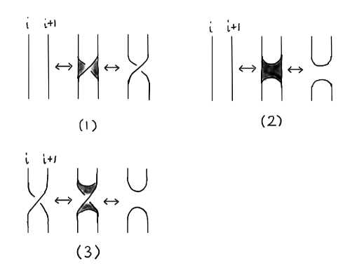
Figure 6. Motion pictures of (1) $\mathbf{1}\leftrightarrow g_{i}$, (2) $\mathbf{1}\leftrightarrow e_{i}$ and (3) $g_{i}\leftrightarrow e_{i}$, where we omit the $j$th strings for $j\neq i,i+1$.

The motion picture presenting (5.4) for $\epsilon=+1$ is as in Fig. 7, and the motion picture presenting (5.5) for $\epsilon=+1$ and $j=i+1$ is as in Fig. 8. For (5.5), the diagram of the BMW surface (or the braided surface) contains a triple point.

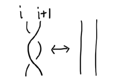
Figure 7. A Reidemeister move of type II presented by $g_{i}g_{i}^{-1}\leftrightarrow\mathbf{1}$, where we omit the $j$th strings for $j\neq i,i+1$.

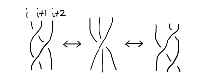
Figure 8. A Reidemeister move of type III presented by $g_{i}g_{j}g_{i}\leftrightarrow g_{j}g_{i}g_{j}$ ($|i-j|=1$), for $j=i+1$, where we omit the $k$th strings for $k\neq i,i+1,i+2$.

The motion pictures presenting (5.6) are as in Fig. 9, and those presenting (5.7) are the mirror image of Fig. 9, where we put the mirror at a horizontal position.

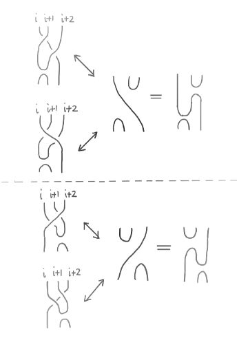
Figure 9. Motion pictures presented by $g_{i}^{\epsilon}g_{j}^{\epsilon}e_{i}\leftrightarrow e_{j}e_{i}$ $(\epsilon\in\{+1,-1\},|i-j|=1)$, where, exchanging $i$ and $j$ if necessary, we denote the set $\{i,j,i+1,j+1\}$ consisting of three integers by $\{i,i+1,i+2\}$, and we omit the $k$th strings for $k\neq i,i+1,i+2$.

The motion pictures presenting (5.8) are as in Fig. 10. The diagrams of $e_{i}e_{j}e_{i}$ and $e_{i}$ $(|i-j|=1)$ are related by an ambient isotopy of the plane.

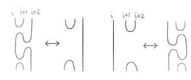
Figure 10. Motion pictures presented by $e_{i}e_{j}e_{i}\leftrightarrow e_{i}$ $(|i-j|=1)$, where, exchanging $i$ and $j$ if necessary, we denote the set $\{i,j,i+1,j+1\}$ consisting of three integers by $\{i,i+1,i+2\}$, and we omit the $k$th strings for $k\neq i,i+1,i+2$.

The motion pictures presenting (5.9)–(5.11) are as in Fig. 11. The diagrams are related by an ambient isotopy of the plane. At some $t\in\mathrm{Int}(I_{4})$, that can be taken as $t=(t_{j-1}+t_{j})/2$, for some $u\in I_{3}$, the diagram of the slice $S$ at $t$ has two crossings in $I_{2}\times\{u\}$ (the top figure) or has one crossing in $I_{2}\times\{u\}$ and $u$ is the $I_{3}$ coordinate of $e_{j}$ (the lower left figure), or $u$ is the $I_{3}$ coordinates of $e_{i}$ and $e_{j}$ (the lower right figure). At $t=(t_{j-1}+t_{j})/2$, the slice of $S$ is not presented by a word in $F_{n}$, while other slices are presented by words in $F_{n}$.

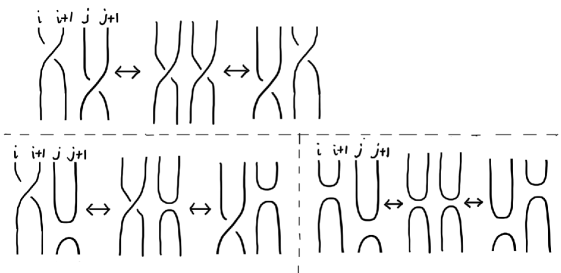
Figure 11. Motion pictures presented by $g_{i}g_{j}\leftrightarrow g_{j}g_{i}$ (top figure), $g_{i}e_{j}\leftrightarrow e_{j}g_{i}$ (lower left figure) and $e_{i}e_{j}\leftrightarrow e_{j}e_{i}$ (lower right figure), $|i-j|>1$, where $i<j$ and we omit the $k$th strings for $k\neq i,i+1,j,j+1$.

The motion picture presenting (5.12) is as in Fig. 12. We paste a disk at a slice of $S$ at some $t\in\mathrm{Int}(I_{4})$, and delete/create the circle component of $e_{i}e_{i}$. The motion pictures presenting (5.13)–(5.14) for $\epsilon=+1$ are as in Fig. 5.

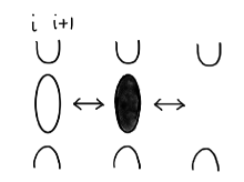
Figure 12. Motion picture presenting $e_{i}e_{i}\leftrightarrow e_{i}$, where we omit the $j$th strings for $j\neq i,i+1$.

Proof of Proposition 5.2.

Let $S$ be a BMW surface satisfying the Conditions (1), (2) and (3) of Definition 5.1. By a fiber-preserving ambient isotopy of $D^{2}\times I_{3}\times I_{4}$, where fiber is $D^{2}\times\{t\}$ $(t\in I_{3}\times I_{4})$, we deform $S$ so that the resulting surface, also denoted by $S$, satisfies the condition as follows: for any $s\in J$, each slice $S\cap(D^{2}\times I_{3}\times\{s\})$ is described by (a’) the union of a BMW tangle and a sufficiently small attached band (resp. disk), that is a saddle band (resp. a minimal/maximal disk), or (b’) the union of a BMW tangle and a sufficiently small attached band that contains the preimage of a branch point. And Condition (2) is that for any interval $[t,t^{\prime}]$ that is a component of $\mathrm{Cl}(I_{4}\backslash N(J))$, the diagrams of $S\cap(D^{2}\times I_{3}\times\{t\})$ and $S\cap(D^{2}\times I_{3}\times\{t^{\prime}\})$ in $I_{2}\times I_{3}$ are related by a finite sequence of Reidemeister moves of types II and III and ambient isotopies of $I_{2}\times I_{3}$ if $S$ is a regular BMW surface, and in addition to these moves, we may have Reidemeister moves of type I if $S$ is a BMW surface. Divide $[0,1]$ into subintervals $[t_{j-1},t_{j}]$ with $0=t_{0}<t_{1}<\cdots<t_{m}=1$ such that (c) each $s\in J$ is the middle point of some $[t_{j-1},t_{j}]$ and (d) for each interval $[t_{j-1},t_{j}]$ that does not contain elements of $J$, we have one of (d1) and (d2) as follow, where $\tau_{j}=S\cap(D^{2}\times I_{3}\times\{t_{j}\})$: (d1) the diagrams of $\tau_{j-1}$ and $\tau_{j}$ in $I_{2}\times I_{3}$ are related by a Reidemeister move, or (d2) the diagrams of $\tau_{j-1}$ and $\tau_{j}$ in $I_{2}\times I_{3}$ are related by an ambient isotopy of $I_{2}\times I_{3}$, that changes words of BMW tangles, or an ambient isotopy of $I_{2}\times I_{3}$ that does not change words of BMW tangles. From now on, we consider the case of $\tau_{j-1}\neq\tau_{j}$. For Case (d2), since the ambient isotopy keeps the BMW tangle form, this is described by a sequence consisting of (5.8) and exchange of two letters: $w_{i}w_{j}\leftrightarrow w_{j}w_{i}$ $(w_{i}\in\{g_{i},g_{i}^{-1},e_{i}\mid i=1,\ldots,n-1\})$ with $|i-j|>1$. We divide $[t_{j-1},t_{j}]$ into subintervals and denote the resulting division by the same notation so that we have (c), and one of (d1) and (d2’) as follow:

1. Each $s\in J$ is the middle point of some $[t_{j-1},t_{j}]$.

2. For each interval $[t_{j-1},t_{j}]$ that does not contain elements of $J$, we have one of (d1) and (d2’) as follow, where $\tau_{j}=S\cap(D^{2}\times I_{3}\times\{t_{j}\})$:

   1. The diagrams of $\tau_{j-1}$ and $\tau_{j}$ in $I_{2}\times I_{3}$ are related by a Reidemeister move.

   2. The diagrams of $\tau_{j-1}$ and $\tau_{j}$ in $I_{2}\times I_{3}$ are related by one of the following: (5.8) and (5.18)–(5.19) in Lemma 5.3, and (5.9)–(5.11).

By Lemma 5.3, (d2’) is presented by a sequence consisting of (5.4) and (5.8)–(5.11).

For $[t_{j-1},t_{j}]$ that contains an element $s\in J$, if the slice at $s$ contains a saddle band or a disk containing the preimage of a branch point, since such bands and disks are sufficiently small, $\tau_{j}$ is obtained from $\tau_{j-1}$ by band surgery described in (5.1)–(5.3). And if the slice at $t$ contains a minimal/maximal disk, since such a disk is sufficiently small, $\tau_{j}$ is obtained from $\tau_{j-1}$ by pasting a disk at $(t_{j-1}+t_{j})/2$ as described by (5.12). For $[t_{j-1},t_{j}]$ that satisfies (d1), seeing the types of the Reidemeister move and the concerning arcs, we have the following cases.

(Case 1) A Reidemeister move is of type II, and the concerning arcs are presented by letters in $\{g_{i},g_{i}^{-1}\mid i=1,\ldots,n-1\}$. In this case, we have (5.4).

(Case 2) A Reidemeister move is of type III, and the concerning arcs are presented by letters in $\{g_{i},g_{i}^{-1}\mid i=1,\ldots,n-1\}$. In this case, the move is one of (5.15)–(5.17) in Lemma 5.3. By Lemma 5.3, it is presented by a sequence consisting of (5.4) and (5.5).

(Case 3) A Reidemeister move is of type II, and the concerning arcs are presented by a letter $e_{i}$ and letters in $\{g_{i},g_{i}^{-1}\mid i=1,\ldots,n-1\}$. The move is when we apply a Reidemeister move of type II to an arc of the pair of arcs of $e_{i}$. In this case, we have (5.6)–(5.7).

(Case 4) A Reidemeister move is of type III, and the concerning arcs are presented by a letter $e_{i}$ for some $i$ and letters in $\{g_{i},g_{i}^{-1},e_{i}\mid i=1,\ldots,n-1\}$. Since $e_{i}$ has no crossings, the arcs of $e_{i}$ are not involved for the Reidemeister move, and so this move is presented by Case 2.

(Case 5) A Reidemeister move is of type II, and the concerning arcs are presented by letters in $\{e_{i}\mid i=1,\ldots,n-1\}$. Since we must keep the BMW tangle form, this case does not exist.

Thus, by taking a division of $[t_{j-1},t_{j}]$ into subintervals and denoting the resulting division of $I_{4}=[0,1]$ by the same notation $0=t_{0}<t_{1}\cdots<t_{m}=1$, for a regular BMW surface, we have $S$ in the required form.

For a non-regular BMW surface, we have an additional move for (d1) as follows.

(Case 6) A Reidemeister move is of type I. Since we must keep the BMW tangle form, together with the definition of a BMW tangle isotopy, this is presented by (5.20)–(5.21) in Lemma 5.3. By Lemma 5.3, it is presented by a sequence consisting of (5.4) and (5.13)–(5.14). Hence, for a BMW surface, we have $S$ in the required form. ∎

Lemma 5.3.

The Reidemeister moves presented by $(\ref{eq5-15})$–$(\ref{eq5-17})$, $(\ref{eq5-18})$, $(\ref{eq5-19})$, $(\ref{eq5-20})$ and $(\ref{eq5-21})$, as follow, are realized by the moves $(\ref{eq5-4})$ and the corresponding $(\ref{eq5-5})$, $(\ref{eq5-9})$, $(\ref{eq5-10})$, $(\ref{eq5-13})$ and $(\ref{eq5-14})$ in Proposition 5.2, respectively:

(5.15) $$g_{i}^{\epsilon}g_{j}^{\epsilon}g_{i}^{\epsilon}\leftrightarrow g_{j}^{-\epsilon}g_{i}^{-\epsilon}g_{j}^{-\epsilon}\quad|i-j|=1,$$

(5.16) $$g_{i}^{\epsilon}g_{j}^{\epsilon}g_{i}^{-\epsilon}\leftrightarrow g_{j}^{-\epsilon}g_{i}^{\epsilon}g_{j}^{\epsilon}\quad|i-j|=1,$$

(5.17) $$g_{i}^{\epsilon}g_{j}^{-\epsilon}g_{i}^{-\epsilon}\leftrightarrow g_{j}^{-\epsilon}g_{i}^{-\epsilon}g_{j}^{\epsilon}\quad|i-j|=1,$$

(5.18) $$g_{i}^{\epsilon}g_{j}^{\delta}\leftrightarrow g_{j}^{\delta}g_{i}^{\epsilon}\quad|i-j|>1,$$

(5.19) $$g_{i}^{\epsilon}e_{j}\leftrightarrow e_{j}g_{i}^{\epsilon}\quad|i-j|>1,$$

(5.20) $$e_{i}\leftrightarrow g_{i}^{\epsilon}e_{i},$$

(5.21) $$e_{i}\leftrightarrow e_{i}g_{i}^{\epsilon},$$

where $\epsilon,\delta\in\{+1,-1\}$, $i,j\in\{1,\ldots,n-1\}$.

Proof.

We have

$$g_{i}^{-1}g_{j}^{-1}g_{i}^{-1} \leftrightarrow g_{i}^{-1}g_{j}^{-1}g_{i}^{-1}(g_{j}g_{i}g_{j}g_{j}^{-1}g_{i}^{-1}g_{j}^{-1})$$

$$= g_{i}^{-1}g_{j}^{-1}g_{i}^{-1}(g_{j}g_{i}g_{j})g_{j}^{-1}g_{i}^{-1}g_{j}^{-1}$$

$$\leftrightarrow g_{i}^{-1}g_{j}^{-1}g_{i}^{-1}(g_{i}g_{j}g_{i})g_{j}^{-1}g_{i}^{-1}g_{j}^{-1}$$

$$= (g_{i}^{-1}g_{j}^{-1}g_{i}^{-1}g_{i}g_{j}g_{i})g_{j}^{-1}g_{i}^{-1}g_{j}^{-1}$$

$$\leftrightarrow g_{j}^{-1}g_{i}^{-1}g_{j}^{-1};$$

hence we have (5.15).

Since we have shown (5.15), We have

$$g_{i}^{\epsilon}g_{j}^{\epsilon}g_{i}^{-\epsilon} \leftrightarrow (g_{j}^{-\epsilon}g_{j}^{\epsilon})g_{i}^{\epsilon}g_{j}^{\epsilon}g_{i}^{-\epsilon}$$

$$= g_{j}^{-\epsilon}(g_{j}^{\epsilon}g_{i}^{\epsilon}g_{j}^{\epsilon})g_{i}^{-\epsilon}$$

$$\leftrightarrow g_{j}^{-\epsilon}(g_{i}^{\epsilon}g_{j}^{\epsilon}g_{i}^{\epsilon})g_{i}^{-\epsilon}$$

$$= g_{j}^{-\epsilon}g_{i}^{\epsilon}g_{j}^{\epsilon}(g_{i}^{\epsilon}g_{i}^{-\epsilon})$$

$$\leftrightarrow g_{j}^{-\epsilon}g_{i}^{\epsilon}g_{j}^{\epsilon};$$

hence we have (5.16).

Similarly, we have

$$g_{i}^{\epsilon}g_{j}^{-\epsilon}g_{i}^{-\epsilon} \leftrightarrow g_{i}^{\epsilon}g_{j}^{-\epsilon}g_{i}^{-\epsilon}(g_{j}^{-\epsilon}g_{j}^{\epsilon})$$

$$= g_{i}^{\epsilon}(g_{j}^{-\epsilon}g_{i}^{-\epsilon}g_{j}^{-\epsilon})g_{j}^{\epsilon}$$

$$\leftrightarrow g_{i}^{\epsilon}(g_{i}^{-\epsilon}g_{j}^{-\epsilon}g_{i}^{-\epsilon})g_{j}^{\epsilon}$$

$$= (g_{i}^{\epsilon}g_{i}^{-\epsilon})g_{j}^{-\epsilon}g_{i}^{-\epsilon}g_{j}^{\epsilon}$$

$$\leftrightarrow g_{j}^{-\epsilon}g_{i}^{-\epsilon}g_{j}^{\epsilon};$$

hence we have (5.17).

We have

$$g_{i}^{-1}g_{j}^{-1} \leftrightarrow g_{i}^{-1}g_{j}^{-1}(g_{i}g_{j}g_{j}^{-1}g_{i}^{-1})$$

$$= g_{i}^{-1}g_{j}^{-1}(g_{i}g_{j})g_{j}^{-1}g_{i}^{-1}$$

$$\leftrightarrow g_{i}^{-1}g_{j}^{-1}(g_{j}g_{i})g_{j}^{-1}g_{i}^{-1}$$

$$= (g_{i}^{-1}g_{j}^{-1}g_{j}g_{i})g_{j}^{-1}g_{i}^{-1}$$

$$\leftrightarrow g_{j}^{-1}g_{i}^{-1};$$

hence we have (5.18) for $\delta=\epsilon$.

Since we have (5.18) for $\delta=\epsilon$,

$$g_{i}^{\epsilon}g_{j}^{-\epsilon} \leftrightarrow (g_{j}^{-\epsilon}g_{j}^{\epsilon})g_{i}^{\epsilon}g_{j}^{-\epsilon}$$

$$= g_{j}^{-\epsilon}(g_{j}^{\epsilon}g_{i}^{\epsilon})g_{j}^{-\epsilon}$$

$$\leftrightarrow g_{j}^{-\epsilon}(g_{i}^{\epsilon}g_{j}^{\epsilon})g_{j}^{-\epsilon}$$

$$= g_{j}^{-\epsilon}g_{i}^{\epsilon}(g_{j}^{\epsilon}g_{j}^{-\epsilon})$$

$$\leftrightarrow g_{j}^{-\epsilon}g_{i}^{\epsilon};$$

hence we have (5.18) for $\epsilon,\delta\{+1,-1\}$.

Since we have (5.10),

$$g_{i}^{-1}e_{j} \leftrightarrow g_{i}^{-1}e_{j}(g_{i}g_{i}^{-1})$$

$$= g_{i}^{-1}(e_{j}g_{i})g_{i}^{-1}$$

$$\leftrightarrow g_{i}^{-1}(g_{i}e_{j})g_{i}^{-1}$$

$$= (g_{i}^{-1}g_{i})e_{j}g_{i}^{-1}$$

$$\leftrightarrow e_{j}g_{i}^{-1};$$

hence we have (5.19).

Since we have (5.13),

$$e_{i} \leftrightarrow (g_{i}^{-1}g_{i})e_{i}$$

$$= g_{i}^{-1}(g_{i}e_{i})$$

$$\leftrightarrow g_{i}^{-1}e_{i};$$

hence we have (5.20). The move (5.21) is shown similarly. ∎

Lemma 5.4.

The Reidemeister moves $(\ref{eq5-6})$, $(\ref{eq5-7})$, $(\ref{eq5-20})$ and $(\ref{eq5-21})$ induce the following moves:

(5.22) $$g_{i}^{\epsilon}g_{j}^{\epsilon}e_{i}\leftrightarrow e_{j}g_{i}^{\delta}g_{j}^{\delta}\quad|i-j|=1,$$

(5.23) $$e_{i}\leftrightarrow g_{i}^{k}e_{i},$$

(5.24) $$e_{i}\leftrightarrow e_{i}g_{i}^{k},$$

where $\epsilon,\delta\in\{+1,-1\}$, $i,j\in\{1,\ldots,n-1\}$, and $k\in\mathbb{Z}$.

Proof.

By (5.6) and (5.7), we have (5.22);

$$g_{i}^{\epsilon}g_{j}^{\epsilon}e_{j}\leftrightarrow e_{j}e_{i}\leftrightarrow e_{j}g_{i}^{\delta}g_{j}^{\delta},$$

where $\epsilon\in\{+1,-1\}$, $|i-j|=1$. And repeating (5.20) and (5.21), we have (5.23) and (5.24), respectively. ∎

Definition 5.5.

Let $\Gamma$ be a finite graph in a 2-disk $E$. Then, $\Gamma$ is a regular BMW chart of degree $n$ if it satisfies the following conditions.

1. The intersection $\Gamma\cap\partial E$ consists of a finite number of points. Though they are vertices of degree one, we call elements of $\Gamma\cap\partial E$ boundary points, and we call a vertex in $\mathrm{Int}(E)$ a vertex of $\Gamma$.

2. Each edge is equipped with a label $\{g_{i},e_{i}\mid i=1,\ldots,n-1\}$ and moreover, if the label is $g_{i}$, then the edge is oriented.

3. Each vertex is of degree 1, 4, 6, called a braid vertex, or of degree 1, 2, 3, 4, 5, called a tangle vertex, as follows; see Figs. 13, 14 and 15:

1. (Braid vertex)

2. A vertex of degree one such that the connecting edge has a label $g_{i}$ for some $i\in\{1,\ldots,n-1\}$ and an orientation. We depict the vertex by a small black disk and call it a black vertex.

3. A vertex of degree 4 such that around the vertex, each pair of diagonal edges has a label in $\{g_{1},\ldots,g_{n-1}\}$ and a coherent orientation, and the labels of the two pairs, $g_{i}$ and $g_{j}$, satisfy $|i-j|>1$. We call the vertex a crossing.

4. A vertex of degree 6 such that around the vertex, the six edges have labels $g_{i},g_{j},g_{i},g_{j},g_{i},g_{j}$ clockwise ($i,j\in\{1,\ldots,n-1\}$), such that $|i-j|=1$. And three consecutive edges have an orientation toward the vertex and the other consecutive edges have an orientation from the vertex. We depict the vertex by a small circle and call it a white vertex.
   

5. (Tangle vertex)

6. A vertex of degree 1 such that the connecting edge has a label $e_{i}$ for some $i\in\{1,\ldots,n-1\}$. We depict the vertex by a small x mark.

7. A vertex of degree 2 such that the connecting edges have labels $e_{i}$ and $g_{i}$ for some $i\in\{1,\ldots,n-1\}$, and the edge with the label $g_{i}$ has an orientation. We depict the vertex by a small x mark.

8. A vertex of degree 4 such that around the vertex, one pair of diagonal edges has a label $g_{i}$ and a coherent orientation, and the other pair of diagonal edges has a label $e_{j}$, or the 4 edges have labels $e_{i}$ and $e_{j}$ alternately, where $i,j\in\{1,\ldots,n-1\}$ and $|i-j|>1$.

9. A vertex of degree 4 such that around the vertex, three edges have a label $e_{i}$ and one edge has a label $e_{j}$ for $i,j\in\{1,\ldots,n-1\}$ with $|i-j|=1$. We depict the vertex by a small square.

10. A vertex of degree 5 such that around the vertex, the edges have labels $g_{i},g_{j},e_{i},e_{i},e_{j}$ clockwise or anti-clockwise for $i,j\in\{1,\ldots,n-1\}$ with $|i-j|=1$, and the pair of edges with the label $g_{i}$ and $g_{j}$ are both oriented toward the vertex or from the vertex. We depict the vertex by a small square.

11. A vertex of degree 3 such that around the vertex, the three edges have the label $e_{i}$ for some $i\in\{1,\ldots,n-1\}$. We depict the vertex by a small x mark.

Further, $\Gamma$ is a BMW chart of degree $n$ if it satisfies the conditions of a regular BMW chart and has additional vertices as follow.

1. A vertex of degree 3 such that two of the connecting edges has a label $e_{i}$ and the other edge has a label $g_{i}$ for some $i\in\{1,\ldots,n-1\}$, and the edge with the label $g_{i}$ has an orientation. We depict the vertex by a small square.

Theorem 5.6.

A regular BMW surface (resp. a BMW surface) has a regular BMW chart (resp. a BMW chart) description. More precisely, from a (regular) BMW surface of degree $n$, we obtain a (regular) BMW chart of degree $n$, and conversely, from a (regular) BMW chart $\Gamma$ of degree $n$, we obtain a surface $S$ that is equivalent to a (regular) BMW surface $S^{\prime}$ of degree $n$ whose (regular) BMW chart presents $S^{\prime}$.

Hence we extend the definition of BMW surfaces as follows, where the surface presented by a BMW chart is given in Section 6.2.

Definition 5.7.

Let $S$ be a surface properly embedded in $D^{2}\times I_{3}\times I_{4}$. Then $S$ is a BMW surface of degree $n$ if it satisfies the conditions given in Definition 5.1, or it is the surface presented by a BMW chart of degree $n$ in $I_{3}\times I_{4}$. Further, a BMW surface is regular if it satisfies the condition of a regular BMW surface given in Definition 5.1, or it is the surface presented by a regular BMW chart.

We show Theorem 5.6 in Section 5.

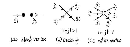
Figure 13. Vertices of a BMW surface: braid vertices.

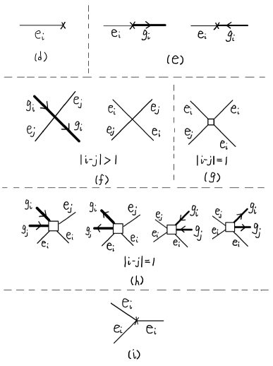
Figure 14. Vertices of a BMW chart: tangle vertices.

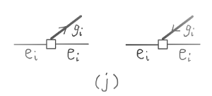
Figure 15. Vertices of a non-regular BMW chart.

6. Proof of Theorem 5.6

In this section, we show Theorem 5.6.

6.1. From a BMW surface to a BMW chart

Let $S$ be a BMW surface of degree $n$ in $D^{2}\times I_{3}\times I_{4}$. We obtain from $S$ a BMW chart $\Gamma$ in $I_{3}\times I_{4}$ as follows. By equivalence, we deform $S$ to a normal form as described in Proposition 5.2. For each $\tau_{j}$ $(j=0,\ldots,m)$, let $w_{1}w_{2}\cdots w_{n_{j}}$ be the word of $\tau_{j}$ $(w_{k}\in\{g_{i},g_{i}^{-1},e_{i}\mid i=1,\ldots,n-1\})$. Take $n_{j}$ points in $I_{3}\times\{t_{j}\}$ and assign $|w_{k}|$ to the $k$th point with respect to the orientation of $I_{3}$, where $|w_{k}|=g_{i}$ if $w_{k}=g_{i}^{\pm 1}$ and $|w_{k}|=e_{i}$ if $w_{k}=e_{i}$. Then, we connect the points in $I_{3}\times\{t_{j-1}\}$ and $I_{3}\times\{t_{j}\}$ by arcs and vertices in $I_{3}\times[t_{j-1},t_{j}]$ in such a way as follows, where $j=1,\ldots,m-1$. We connect the points that do not concern (5.1)–(5.14) by mutually disjoint parallel arcs, and those concerning (5.1)–(5.3), (5.5)–(5.14) by arcs connected with a vertex in $I_{3}\times\{(t_{j-1}+t_{j})/2\}$. Now, the points concerning (5.4) are a pair of points in $I_{3}\times\{t_{j-1}\}$ or $I_{3}\times\{t_{j}\}$; and we connect the pair of points by a simple arc. By regarding the points in $I_{3}\times\{t_{j}\}$ $(j=1,\ldots,m-1)$ as inner points of edges, we obtain a graph. Assign each edge with the label of the belonging points, and moreover, if the point in $I_{3}\times\{t_{j}\}$ comes from a letter $g_{i}$ (resp. $g_{i}^{-1}$) in $\tau_{j}$, then assign the edge with an orientation coherent with that of $I_{4}$ (resp. opposite to that of $I_{4}$). Then, by depicting vertices by those of a BMW chart, we have a BMW chart of degree $n$.

Remark 6.1.

Let $p:D^{2}\times I_{3}\times I_{4}\to I_{2}\times I_{3}\times I_{4}$ be a regular projection and let $D=p(S)$ be the diagram of $S$. Then, a double point curve of $D$ is projected by the projection $p^{\prime}:I_{2}\times I_{3}\times I_{4}\to I_{3}\times I_{4}$ to an edge of $\Gamma$ with a label in $\{g_{i}\mid i=1,\ldots,n-1\}$. A triple point of $D$ is projected by $p^{\prime}$ to a white vertex, and a branch point of $D$ is projected to a black vertex.

6.2. From a BMW chart to the surface presented by the chart

Given a BMW chart $\Gamma$ of degree $n$ in $I_{3}\times I_{4}$, we construct the surface $S$ in $D^{2}\times I_{3}\times I_{4}$ presented by $\Gamma$ in such a way as follows. For a (regular) BMW surface, we often call its (regular) BMW chart simply a (regular) chart.

We construct the surface $S$ locally as follows. We take a division of $I_{3}\times I_{4}$ into a finite number of disks such that each disk $E$ satisfies the following:

1. The boundary $\partial E$ does not contain vertices of $\Gamma$, and $\Gamma\cap\partial E$ consists of transverse intersection points of edges of $\Gamma$ and $\partial E$.

2. The chart $\Gamma\cap E$ contains exactly one vertex and arcs of its connecting edges, or exactly one arc of an edge.

We remark that when $\partial E\cap\partial(I_{3}\times I_{4})\neq\emptyset$, we regard boundary points of $\Gamma$ in $\partial E$ as transverse intersection points of edges of $\Gamma$ and $\partial E$. Then there exists an orientation-preserving homeomorphism $f:E\to I_{3}\times I_{4}$ such that $\Gamma^{\prime}=f(\Gamma\cap E)$ is the chart of a BMW surface $S^{\prime}$ in a normal form, that is given later. Then, we construct $S\cap E$ as the image of $S^{\prime}$ by $\mathrm{id}_{D^{2}}\times f^{-1}:D^{2}\times I_{3}\times I_{4}\to D^{2}\times E$.

We construct $S^{\prime}$ in $D^{2}\times I_{3}\times I_{4}$ as follows. By an orientation-preserving homeomorphism $f:E\to I_{3}\times I_{4}$, we deform $\Gamma\cap E$ to $\Gamma^{\prime}$ so that the intersection $\Gamma^{\prime}\cap(I_{3}\times\{t\})$ $(t\in I_{4})$ consists of a finite number of points such that each point is one of the following.

1. A vertex.

2. A transverse intersection point of an edge of $\Gamma$ and $I_{3}\times\{t\}$.

And by rotating a vertex if necessary, and taking a new division of $I_{3}\times I_{4}$, we have a situation that each vertex is the one coming from a BMW surface in a normal form of Proposition 5.2. Then, take $\tau_{j}=w_{1}w_{2}\cdots w_{m_{j}}\in F_{n}$ $(j=0,1)$, where $m_{j}$ is the number of points of $\Gamma\cap(I_{3}\times\{j\})$ $(j=0,1)$, and $w_{k}=g_{i}$ (resp. $g_{i}^{-1}$) if the $k$th point with respect to the direction of $I_{3}$ is a point of an edge with the label $g_{i}$ and an orientation coherent with that of $I_{4}$ (resp. an orientation opposite to that of $I_{4}$), and $w_{k}=e_{i}$ if the $k$th point is a point of an edge with the label $e_{i}$ ($k=1,\ldots,m_{j}$). And using $\tau_{0}$ and $\tau_{1}$, we construct a BMW surface of degree $n$ as in Proposition 5.2.

Thus we have the surface $S$ in $D^{2}\times I_{3}\times I_{4}$ presented by a chart $\Gamma$.

Remark 6.2.

When we extend the definition of BMW surfaces to Definition 5.7, by a similar argument as in Section 6.1, from a BMW surface we obtain a BMW chart, and from a BMW chart $\Gamma$, we obtain a BMW surface whose chart is $\Gamma$.

6.3. From the presented surface to a BMW surface

Let $S$ be the surface in $D^{2}\times I_{3}\times I_{4}$ presented by a BMW chart $\Gamma$ of degree $n$ in $I_{3}\times I_{4}$. The surface $S$ is equivalent to the surface presented by a chart of degree $n$, also denoted by $\Gamma$, in the following form, where $0=t_{0}<t_{1}<\ldots<t_{m}=1$ for some $m$:

1. The chart $\Gamma$ and $\partial I_{3}\times I_{4}$ are disjoint, that is, $\Gamma\cap(\partial I_{3}\times I_{4})=\emptyset$.

2. For any $t\in I_{4}\backslash\partial I_{4}$, the intersection $\Gamma\cap(I_{3}\times\{t\})$ consists of a finite number of points such that one point is (a) or (c), and the other points are (b):

   1. A vertex.

   2. A transverse intersection point of an edge of $\Gamma$ and $I_{3}\times\{t\}$.

   3. A minimal point or a maximal point of a curving edge with respect to the $I_{4}$ direction.

3. Each $\Gamma\cap(I_{3}\times[t_{j-1},t_{j}])$ $(j=1,\ldots,m)$ contains exactly one vertex, or one minimal/maximal point of Case (c) in (2).

Though each $S\cap(D^{2}\times I_{3}\times[t_{j-1},t_{j}])$ is a BMW surface of Definition 5.1, we must see that $S$ is equivalent to a BMW surface as a whole. We remark that for a BMW surface in a normal form as in Proposition 5.2, its chart has no edges that form arcs as described in Case (c). Let $\Gamma^{\prime}$ be a BMW chart obtained from $\Gamma$ by exchanging each arc of Case (c) that is as in the left figure of Fig. 16 (or its mirror image where we put the mirror in a vertical position) to a subgraph (or its mirror image) as in the right figure of Fig. 16, where, in Fig. 16, the horizontal direction is the $I_{4}$ direction. The graph as in the right figure of Fig. 16 consists of a pair of arcs $c_{1},c_{2}$ and one edge $c_{3}$ such that $c_{3}$ is connected with a vertex of degree one and $c_{1},c_{2},c_{3}$ are connected with a vertex of degree three. Then, the surface $S^{\prime}$ constructed from $\Gamma^{\prime}$ is a BMW surface in a normal form: thus $S^{\prime}$ is a BMW surface whose chart $\Gamma^{\prime}$ presents $S^{\prime}$. By Proposition 6.3, the surface $S$ in question is equivalent to $S^{\prime}$. Hence we have the required result.

Proposition 6.3.

The surfaces presented by the BMW charts of degree $n$ as in the left figure and the right figure of Fig. 16 are equivalent, in the sense of equivalence in Definition 5.1.

From a cylinder $D^{2}\times I$, we obtain a solid torus $D^{2}\times S^{1}$ by identifying $D^{2}\times\{0\}$ and $D^{2}\times\{1\}$. We denote the map $D^{2}\times I\to D^{2}\times S^{1}$ by $f$. For a BMW tangle $\tau$ in $D^{2}\times I$, the closure of $\tau$ in $D^{2}\times S^{1}$ is the image $f(\tau)$.

Proof of Proposition 6.3.

We denote by $E$ the disk in which BMW charts are drawn. The surface $S$ presented by the chart as in the left figure in Fig. 16 is the one as depicted in the middle figure of Fig. 17, that is obtained by deforming the surface whose slices are $e_{i}$ as in the left figure in Fig. 17 by an ambient isotopy of $D^{2}\times E$ induced from that of $E$. The surface $S$ consists of a pair of disks whose boundaries are the closure of the BMW tangle $e_{i}e_{i}$ in the solid torus $D^{2}\times\partial E$, where we ignore other components coming from the $j$th strings for $j\neq i,i+1$. This surface $S$ is related with the surface $S^{\prime}$ as in the right figure of Fig. 17 by an isotopy of surfaces. Hence, $S$ is equivalent to $S^{\prime}$, that is the BMW surface presented by the chart as in the right figure of Fig. 16. Hence we have the required result. ∎

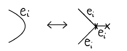
Figure 16. BMW charts of degree $n$ whose associated surfaces are equivalent, where $i\in\{1,\ldots,n-1\}$ and we omit the 2-disks in which the charts are drawn.

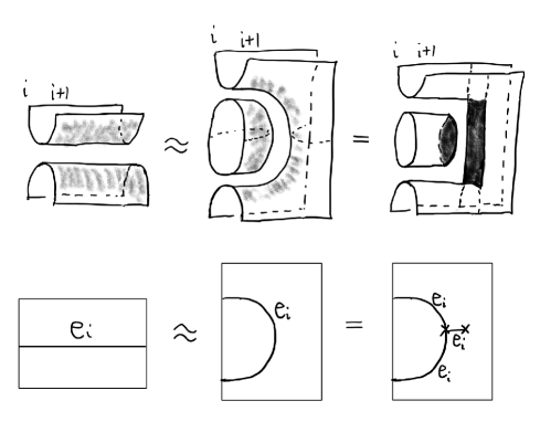
Figure 17. The surfaces presented by BMW charts in Fig. 16 are equivalent, where we omit other components coming from the $j$th strings for $j\neq i,i+1$.

Proof of Theorem 5.6.

By the argument in Sections 6.1–6.3, we have the required result. ∎

7. BMW chart moves

In this section, we give the definition of BMW chart moves, that are local moves of BMW charts of degree $n$ such that their associated BMW charts are equivalent. This includes C-moves of charts of 2-dimensional braids [3, 4, 6]. See also [7] for charts and C-moves for (non-simple) braided surfaces.

Definition 7.1.

Let $\Gamma$ and $\Gamma^{\prime}$ be (regular) BMW charts of degree $n$ in a 2-disk $D^{2}$. Then, a BMW chart move, or simply a chart move or a C-move, is a local move in a 2-disk $E\subset D^{2}$ such that $\Gamma$ (resp. $\Gamma^{\prime}$) is changed to $\Gamma^{\prime}$ (resp. $\Gamma$), satisfying the following.

1. The boundary $\partial E$ does not contain vertices of $\Gamma$ and $\Gamma^{\prime}$, and $\Gamma\cap\partial E$ (resp. $\Gamma^{\prime}\cap\partial E$) consists of transverse intersection points of edges of $\Gamma$ (resp. $\Gamma^{\prime}$) and $\partial E$.

2. The charts are identical in the complement of $E$: $\Gamma\cap(D^{2}\backslash E)=\Gamma^{\prime}\cap(D^{2}\backslash E)$.

3. The charts in $E$, $\Gamma\cap E$ and $\Gamma^{\prime}\cap E$, satisfy one of the following.

   1. The charts $\Gamma\cap E$ and $\Gamma^{\prime}\cap E$ consist of vertices and edges with labels in $\{g_{i}\mid i=1,\ldots,n-1\}$ and satisfy one of the following three cases:

      1. The charts $\Gamma\cap E$ and $\Gamma^{\prime}\cap E$ do not contain black vertices; see the top figure in Fig. 18 for examples.

      2. The charts $\Gamma\cap E$ and $\Gamma^{\prime}\cap E$ are as depicted in the middle figure in Fig. 18.

      3. The charts $\Gamma\cap E$ and $\Gamma^{\prime}\cap E$ are as depicted in the bottom figure in Fig. 18.

      We call the chart moves braid chart moves of type I, II, III, or simply CI, CII, CIII-moves, respectively.

   2. The charts $\Gamma\cap E$ and $\Gamma^{\prime}\cap E$ satisfy the following conditions, where we assume $E=I\times[0,1]$ and boundary points of $\Gamma\cap E$ and $\Gamma^{\prime}\cap E$ are in $I\times\{0,1\}$, that is, $\Gamma\cap(\{0,1\}\times[0,1])=\Gamma^{\prime}\cap(\{0,1\}\times[0,1])=\emptyset$.

      1. Each of $\Gamma\cap E$ and $\Gamma^{\prime}\cap E$ is in the form of $\Gamma_{0}\cup(-\Gamma_{0}^{*})$ for a chart $\Gamma_{0}$ in $I\times[0,1/2]$, where $-\Gamma_{0}^{*}$ is the orientation-reversed mirror image of $\Gamma_{0}$ with the mirror at $I\times\{1/2\}$.

      2. The charts do not contain vertices of degree one or two, or vertices of type (i).

      3. For any $t\in[0,1]$, $\Gamma\cap(I\times\{t\})$ and $\Gamma^{\prime}\cap(I\times\{t\})$ do not contain a pair of adjacent points coming from edges with the label $e_{i}$ for $i=1,\ldots,n-1$.

      In particular, we can take $\Gamma^{\prime}\cap E$ as a chart consisting only of parallel arcs of edges connecting boundary points. See Fig. 19 for examples.

   3. The charts $\Gamma\cap E$ and $\Gamma^{\prime}\cap E$ are as in Fig. 16.

      We call the chart moves of (b) and (c) tangle chart moves.

See Definition 8.5 for C-moves for BMW charts with additional vertices of types (k), (i’) and (j’) defined in Definitions 8.2 and 8.4.

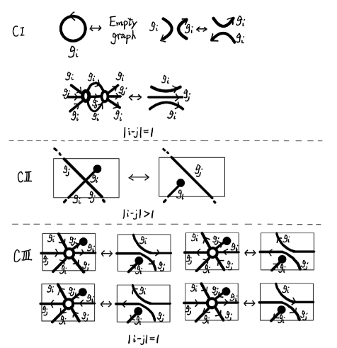
Figure 18. BMW chart moves: (a) braid chart moves of types I, II and III, or CI, CII, and CIII moves.

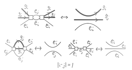
Figure 19. Examples of BMW chart moves of (b).

Definition 7.2.

Let $\Gamma$ and $\Gamma^{\prime}$ be (regular) BMW charts of degree $n$ in a 2-disk $D^{2}$. We say that $\Gamma$ and $\Gamma^{\prime}$ are BMW chart-move equivalent or simply C-move equivalent if they are related by a finite sequence of BMW chart moves and ambient isotopies of $D^{2}$.

We have the following theorem. For 2-dimensional braids, the converse of Theorem 7.3 holds true [3, 5, 4]; so we have Question (1) in Section 9.

Theorem 7.3.

Two (regular) BMW surfaces of degree $n$ are equivalent if their presenting charts are BMW chart-move equivalent.

Proof.

Let $S$ and $S^{\prime}$ be BMW surfaces of degree $n$ such that $S$ is obtained from $S^{\prime}$ by a BMW chart move $\mathcal{X}$. If $\mathcal{X}$ is a braid chart move, then $S$ and $S^{\prime}$ are equivalent by the theory of C-move equivalence of surface braids; because the monodromy doesn’t change; see [3, 4]. If $\mathcal{X}$ is a tangle chart move of type (b), then $S$ and $S^{\prime}$ are equivalent by an argument as follows. We assume that $S=S\cap E$ and $S^{\prime}=S^{\prime}\cap E$. It suffices to consider the case when $\Gamma^{\prime}$ consists only of edges and boundary points. By Conditions (b2) and (b3), we see that $S$ and $S^{\prime}$ do not contain bands nor disks in each slice. Hence, $S\cap(I\times[0,1/2])$ is the trace of a BMW tangle $\tau$ in $D^{2}\times I$ by a BMW tangle isotopy (or regular ambient isotopy) $\{f_{u}\}_{u\in[0,1/2]}$. Put $\tau_{u}=f_{u}(\tau)$ $(u\in[0,1/2])$. By Condition (b1),

$$S=\left(\bigcup_{u\in[0,1/2]}\tau_{u}\times\{u\}\right)\cup\left(\bigcup_{u\in[1/2,1]}\tau_{1-u}\times\{u\}\right).$$

And

$$S^{\prime}=\bigcup_{u\in[0,1]}\tau\times\{u\}.$$

Then, put

$$\tau_{u,t}=\begin{cases}\tau_{u(1-t)}&u\in[0,1/2]\\ \tau_{(1-u)(1-t)}&u\in[1/2,1],\end{cases}$$

where $t\in[0,1]$.

Put $S_{t}=\cup_{u\in[0,1]}\tau_{u,t}\times\{u\}$. Then, $\{S_{t}\}_{t\in[0,1]}$ is an isotopy of surfaces connecting $S$ and $S^{\prime}$. Thus $S$ and $S^{\prime}$ are equivalent. If $\mathcal{X}$ is a tangle chart move of type (c), by Proposition 6.3, $S$ and $S^{\prime}$ are equivalent. ∎

8. Additional types of vertices of BMW charts

In this section, we introduce additional types of vertices of BMW charts.

By Lemma 5.4, we have the following Proposition. This proposition is also shown by drawing a chart.

Proposition 8.1.

The trace of the BMW tangle of degree $n$ presented by (5.22) in Lemma 5.4 forms a (regular) BMW surface of degree $n$.

Hence we introduce another type of vertices.

Definition 8.2.

For a (regular) BMW chart of degree $n$, we define a new type of vertices of degree 6 as in Fig. 20:

1. A vertex of degree 6 such that around the vertex, the edges have the labels $g_{i},g_{j},e_{i},e_{i},g_{j},g_{i}$ clockwise for $i,j\in\{1,\ldots,n-1\}$ with $|i-j|=1$, and each pair of consecutive edges with the labels $g_{i}$ and $g_{j}$ has an orientation toward the vertex or from the vertex. We depict the vertex by a small square.

And we define the associated BMW surface as the trace of the BMW tangle $g_{i}^{\epsilon}g_{j}^{\epsilon}e_{i}\in F_{n}$ by the ambient isotopy relating $g_{i}^{\epsilon}g_{j}^{\epsilon}e_{i}$ and $e_{j}g_{i}^{\delta}g_{j}^{\delta}$ $(\epsilon,\delta\{+1,-1\})$, presented by (5.22).

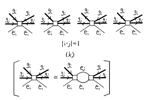
Figure 20. An additional type of vertices of a BMW chart.

By the same argument as in the proof of Proposition 6.3, we have the following proposition. A finite graph is called a tree if it contains no cycles.

Proposition 8.3.

Let $m$ be an arbitrary positive integer. Let $\Gamma$ and $\Gamma^{\prime}$ be BMW charts of degree $n$ in the form of a tree consisting of $m$ vertices of type $(i)$ (resp. type $(j)$ such that the vertices are connected with edges labeled with $e_{i}$). Then the associated BMW surfaces are equivalent.

Proof.

First we show the result when $m=2$. When $\Gamma$ and $\Gamma^{\prime}$ consist of type (i), then all the possible BMW surfaces are those presented by $(e_{i}e_{i})e_{i}\to e_{i}e_{i}\to e_{i}$ and $e_{i}(e_{i}e_{i})\to e_{i}e_{i}\to e_{i}$, where each deformation is $e_{i}e_{i}\to e_{i}$ of (5.12) $(i\in\{1,\ldots,n-1\})$. These BMW surfaces are equivalent, since we can deform them to have the pasting disks in one slice. We also remark that the BMW surfaces both consist of 4 disks whose boundaries are the closure of $e_{i}e_{i}e_{i}e_{i}$. When $\Gamma$ and $\Gamma^{\prime}$ consist of type (j), then the possible BMW surfaces are those presented by $(e_{i}g_{i}^{\epsilon})e_{i}g_{i}^{\delta}\to e_{i}(e_{i}g_{i}^{\delta})\to e_{i}e_{i}\to\mathbf{1}$ and $e_{i}(g_{i}^{\epsilon}e_{i})g_{i}^{\delta}\to e_{i}e_{i}g_{i}^{\delta}=e_{i}(e_{i}g_{i}^{\delta})\to e_{i}e_{i}\to\mathbf{1}$, where each deformation is $g_{i}^{\epsilon}e_{i}\to e_{i}$ or $e_{i}g_{i}^{\epsilon}\to e_{i}$ of (5.20) and (5.21) ($\epsilon,\delta\in\{+1,-1\}$, $i\in\{1,\ldots,n-1\}$). They are equivalent, since the BMW surfaces both consist of 2 disks whose boundaries are the closure of $e_{i}g_{i}^{\epsilon}e_{i}g_{i}^{\delta}$. By a similar argument, for an arbitrary $m$, we have the required result. ∎

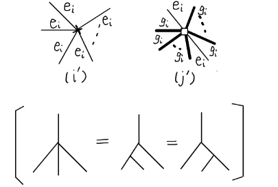
Figure 21. Additional types of vertices of a BMW chart. In the right figure of type (j’), we omit orientations of edges with the label $g_{i}$.

So we introduce vertices of a chart as in Fig. 21.

Definition 8.4.

Let $m$ be an arbitrary integer greater than two. We define new types of vertices of degree $m$ of a BMW chart of degree $n$ as in Fig. 21:

1. A vertex of degree $m$ such that around the vertex, the edges have the label $e_{i}$ for some $i\in\{1,\ldots,n-1\}$. We depict the vertex by a small x mark.

2. A vertex of degree $m$ such that around the vertex, two of the edges have the label $e_{i}$ and the other edges have the label $g_{i}$ for some $i\in\{1,\ldots,n-1\}$ such that each edge with the label $g_{i}$ has an orientation toward the vertex or from the vertex. We depict the vertex by a small square.

Let $\Gamma^{\prime}$ be the BMW surface of degree $n$ in a 2-disk $E$ that is a neighborhood of a vertex of type (i’) (resp. (j’)). Then we define the BMW surface associated with $\Gamma^{\prime}$ as that presented by a BMW chart $\Gamma$ of degree $n$ in $E$ with $\Gamma\cap\partial E=\Gamma^{\prime}\cap\partial E$ such that $\Gamma$ is in the form of a tree consisting of vertices of type (i) (resp. type (j) such that the vertices are connected with edges labeled with $e_{i}$).

When we include vertices of types (k), (i’) and (j’), Condition (b2) of Definition 7.1 is changed to (b2’) as follows, so that Theorem 7.3 holds true:

Definition 8.5.

Let $\Gamma$ and $\Gamma^{\prime}$ be (regular) BMW charts of degree $n$ in a 2-disk $D^{2}$, including vertices of types (k), (i’) and (j’). Then, a BMW chart move, or simply a chart move or a C-move, is a local move as defined in Definition 7.1, where Condition (b2) is changed to (b2’) as follows:

1. The charts do not contain vertices of degree one or two, or vertices of type (i’).

9. Further questions

We close this paper by enumerating questions, that we will investigate in future.

1. We don’t have a sufficient set of BMW chart moves to have the converse of Theorem 7.3. What other types of BMW chart moves are there?

2. What surfaces does each subgraph of a BMW chart present?

3. What “normal form” like ribbon charts are there for BMW charts, and what form do have BMW surfaces?

4. We can consider knotted surfaces in the form of closures of BMW surfaces, where we have two types of closures: closures as in the case of surface braids, and plat closures. What properties can we show for knotted surfaces using BMW surfaces?

5. The equivalence of BMW surfaces does not preserve the “position” of components without boundary. For example, the BMW surface of degree 4 presented by $e_{1}e_{3}\to e_{1}e_{1}e_{3}\to e_{1}e_{3}$ is equivalent to the one presented by $e_{1}e_{3}\to e_{1}e_{3}e_{3}\to e_{1}e_{3}$. How can we define an equivalence relation of BMW surfaces that preserves the “position” of components without boundary?

References

- [1] J. S. Birman, H. Wenzl, Braids, link polynomial and a new algebra, Trans. Amer. Math. Soc. 313 (1989) 249–273.
- [2] J. S. Carter, S. Kamada, M. Saito, Surfaces in 4-space, Encyclopaedia of Mathematical Sciences 142, Low-Dimensional Topology III, Berlin, Springer-Verlag, 2004.
- [3] S. Kamada, Braid and Knot Theory in Dimension Four, Math. Surveys and Monographs 95, Amer. Math. Soc., 2002.
- [4] S. Kamada, An observation of surface braids via chart description, J. Knot Theory Ramifications 5 (1996), no. 4, 517–529.
- [5] S. Kamada, A characterization of groups of closed orientable surfaces in 4-space, Topology 33 (1994) 113–122.
- [6] S. Kamada, Surfaces in of braid index three are ribbon, J. Knot Theory Ramifications 1 (1992), no. 2, 137–160.
- [7] S. Kamada, T. Matumoto, Chart descriptions of regular braided surfaces, Topology Appl. 230 (2017), 218–232.
- [8] L. H. Kauffman, An invariant of regular isotopy, Trans. Amer. Math. Soc. 318 (1990), no. 2, 417–471.
- [9] A. Kawauchi, A Survey of Knot Theory, Birkhäuser Verlag, Basel, 1996.
- [10] H. R. Morton, A basis for the Birman-Wenzl algebra, arXiv:1012.3116
- [11] J. Murakami, The Kauffman polynomial of links and representation theory, Osaka J. Math. 24 (1987) 745–758.