A supervised deep learning method for nonparametric density estimation

Abstract

Nonparametric density estimation is an unsupervised learning problem. In this work we propose a two-step procedure, that casts the density estimation problem in the first step into a supervised regression problem. The advantage is that we can afterwards apply supervised learning methods. Compared to the standard nonparametric regression setting, the proposed procedure creates, however, dependence among the training samples. To derive statistical risk bounds, one can therefore not rely on the well-developed theory for i.i.d. data. To overcome this, we prove an oracle inequality for this specific form of data dependence. As an application, it is shown that under a compositional structure assumption on the underlying density the proposed two-step method achieves faster convergence rates. A simulation study illustrates the finite sample performance.

Keywords: Neural networks, nonparametric density estimation, statistical estimation rates, (un)supervised learning.

MSC 2020: Primary: 62G07; secondary 68T07

1 Introduction

Machine learning distinguishes between supervised and unsupervised learning tasks [9, 37]. In the supervised framework, the dataset consists of input-output pairs. No outputs are observed in the unsupervised setting. For supervised learning, classical examples are regression and classification; for unsupervised learning, commonly encountered problems are density estimation and clustering. The apparent difference between supervised and unsupervised tasks results in methods that either apply to the supervised or to the unsupervised framework. Of course, neural nets can be applied in both scenarios but the underlying methodology is unrelated: In the supervised context, deep learning is applied to reconstruct the function mapping the inputs to the outputs; in the unsupervised framework, neural networks are employed for feature extraction, e.g. by making use of variational autoencoders [25].

In this article, we show how unsupervised multivariate density estimation can be cast into a supervised regression problem. For that, we generate suitable response variables from the data in a first step. Rewriting the problem as supervised learning task allows us to borrow strength from supervised learning methods. We demonstrate this by fitting deep ReLU networks. In the theoretical deep learning literature, it has been shown that supervised deep networks can outperform other methods if the target function exhibits some compositional structure. Making the link to supervised learning allows us to exploit this property also for density estimation. This is highly desirable as compositional structure is frequently imposed in modelling of densities. Examples include copula models [1, 38] and Bayesian network models [30], see also Section 4.

Theorem 3.1 is the main theoretical contribution and establishes an oracle inequality for supervised regression methods applied to nonparametric density estimation. The key technical difficulty in the proof is to deal with the dependence incurred by generating the response variables in the first step of the proposed method. To control the dependence, we use a Poissonization argument. Applying the derived oracle inequality, we show in Theorem 3.4 that deep ReLU networks can obtain fast convergence rates, given that the underlying density has a compositional structure. For sufficiently smooth densities, the convergence rates are, up to logarithmic factors in the sample size, the same as the recently obtained minimax rates in the nonparametric regression model under compositional structure on the regression function, [46]. But there are also smoothness regimes, where the convergence rate is slower by a polynomial order in the sample size if compared to the nonparametric regression case. This is due to the first step in the construction of the estimator that transforms the density estimation problem into a supervised regression problem. But still then there are scenarios where the convergence rate is considerably faster than doing off-the-shelf kernel density estimation without taking the underlying compositional structure of the density into account.

The proposed two-step procedure is related to Lindsey’s method which transforms parametric estimation in exponential families into a Poisson regression problem [34, 33, 18]. The first step of this method discretizes the sample space into disjoint bins. The bin counts follow a multinomial distribution that is then approximated by the Poisson distribution. Assuming Poisson distributed bin counts, maximum likelihood estimation of the parameters results then in a Poisson regression problem. A benefit of Lindsey’s transformation is that the normalization constant of the exponential family vanishes. This constant is an integral over the entire domain and hard to compute in high dimensions [36, 20]. While Lindsey’s method returns one observation per bin and has been formulated for exponential families, the proposed method in this work focuses on nonparametric densities and artificially creates a supervised dataset by computing a response vector for each of the datapoints. Approximation of the bin counts by the Poisson distribution occurs in our approach in the proof.

The paper is structured as follows. Section 2 describes the construction of suitable response variables from the data. In Section 3 we present a suitable oracle inequality for non-i.i.d. data. Furthermore, we provide convergence rates in the case that the regression estimator is a deep neural network and the underlying density are compositional functions. In Section 4 we shortly discuss some density models that exhibit compositional structure. A small (exploratory) simulation is provided in Section 5. All proofs are deferred to the Appendix.

1.1 Notation

We denote vectors and vector valued functions by bold letters. For a vector $\mathbf{x}=(x_{1},\ldots,x_{k})^{\top}$ we define $|\mathbf{x}|_{\infty}=\max_{i=1,\ldots,k}|x_{i}|$, $|\mathbf{x}|_{1}=\sum_{i=1}^{k}|x_{i}|.$ and $|\mathbf{x}|_{0}=\sum_{i=1}^{k}\mathbbm{1}_{\{x_{i}\neq 0\}}$. For partial derivatives we use multi-index notation, that is if $\bm{\alpha}\in\mathbb{N}^{d}$ we use the notation $\partial^{\bm{\alpha}}:=\partial^{\alpha_{1}}\ldots\partial^{\alpha_{d}}.$ We denote the $L^{\infty}$-norm for a function $f:\mathcal{D}\rightarrow\mathbb{R}$ as $\|f\|_{L^{\infty}(\mathcal{D})}$. When there is no ambiguity about the domain $\mathcal{D}$, we simply write $\|f\|_{\infty}$. For a real number $x\in\mathbb{R},$ $\lfloor{x}\rfloor$ is the largest integer $<x$ and $\lceil{x}\rceil$ is the smallest integer $\geq x$. For two sequences $(a_{n})_{n}$ and $(b_{n})_{n}$, we write $a_{n}\lesssim b_{n}$ if there exists a constant $C$ such that $a_{n}\leq Cb_{n}$ for all $n$. Moreover, $a_{n}\asymp b_{n}$ means that $a_{n}\lesssim b_{n}$ and $b_{n}\lesssim a_{n}$.

2 Conversion into supervised learning problem

We consider nonparametric density estimation on the hypercube $[0,1]^{d}$, where we observe $2n$ i.i.d. vectors $\mathbf{X}_{i}\in[0,1]^{d}$ which are distributed according to an unknown density $f_{0}$ from a nonparametric class. The density estimation problem is to recover this density $f_{0}$ from the data $(\mathbf{X}_{i})_{i=1}^{2n}.$ Here the sample size $2n$ is chosen for notational convenience, as we will do data splitting. Half of the data are used to compute an undersmoothed kernel density estimator. From that we construct response variables $Y_{i}$ for the remaining data. In a last step, we fit a neural network to the resulting regression problem. The response variables $Y_{i}$ can be interpreted as noisy versions of $f_{0}(\mathbf{X}_{i}),$ such that the regression estimator then yields an estimator for the underlying density $f_{0}.$ It is convenient to denote the $n$ data points used for the kernel density estimator by $\mathbf{X}_{1}^{\prime},\ldots,\mathbf{X}_{n}^{\prime},$ and the $n$ data points for the regression step by $\mathbf{X}_{1},\ldots,\mathbf{X}_{n}.$

The multivariate kernel density estimator based on the subsample $\mathbf{X}_{1}^{\prime},\ldots,\mathbf{X}_{n}^{\prime}$ with $\mathbf{X}_{\ell}^{\prime}=(X^{\prime}_{\ell,1},\ldots,X^{\prime}_{\ell,d})^{\top}$ is defined by

$$\widehat{f}_{\operatorname{KDE}}(\mathbf{x}):=\frac{1}{nh_{n}^{d}}\sum_{\ell=1}^{n}\prod_{r=1}^{d}K\left(\frac{X^{\prime}_{\ell,r}-x_{r}}{h_{n}}\right),$$ (2.1)

with $h_{n}$ the bandwidth and $K:\mathbb{R}\to\mathbb{R}$ the kernel. We choose a sequence $h_{n}$ satisfying $(\log(n)/n)^{1/d}\leq h_{n}\leq 2(\log(n)/n)^{1/d}$ and such that $h_{n}^{-1}$ is a positive integer for all $n>1$. Existence of such a sequence is guaranteed by Lemma 3.2. The fact that $h_{n}^{-1}$ is a positive integer allows us to partition $[0,1]$ into $h_{n}^{-1}$ disjoint intervals of length $h_{n}.$ This construction undersmooths and does not require knowledge of the true smoothness.

For $i=1,\ldots,n,$ define

$$Y_{i}:=\widehat{f}_{\operatorname{KDE}}(\mathbf{X}_{i}).$$ (2.2)

Setting $\epsilon_{i}:=Y_{i}-f_{0}(\mathbf{X}_{i}),$ we obtain the regression model

$$Y_{i}=f_{0}(\mathbf{X}_{i})+\epsilon_{i},\quad i=1,\ldots,n.$$ (2.3)

Although the notation seems to suggest that this is the standard nonparametric regression framework, the pairs $(\mathbf{X}_{1},Y_{1}),\ldots,(\mathbf{X}_{n},Y_{n})$ are dependent and thus not i.i.d. To deal with this dependence is the main technical challenge in the analysis of the proposed method.

The least squares estimator $\widehat{f}_{n}$ over a function class $\mathcal{F}$ for the density $f_{0}$ is defined as any global minimizer of the least squares loss

$$\widehat{f}_{n}\in\operatorname*{arg\,min}_{f\in\mathcal{F}}\frac{1}{n}\sum_{i=1}^{n}(Y_{i}-f(\mathbf{X}_{i}))^{2}.$$

Due to the nonconvex energy landscape, neural network training usually does not find the global minimum. The difference between training error of the estimator and training error of the global minimum is commonly referred to as optimization error. For any estimator $\widehat{f}$ taking values in a function class $\mathcal{F},$ and data generated from the nonparametric regression model with regression function $f_{0},$ we consider here the optimization error

$$\Delta_{n}(\widehat{f},f_{0}):=\mathbb{E}_{f_{0}}\left[\frac{1}{n}\sum_{i=1}^{n}(Y_{i}-\widehat{f}(\mathbf{X}_{i}))^{2}-\min_{f\in\mathcal{F}}\frac{1}{n}\sum_{i=1}^{n}(Y_{i}-f(\mathbf{X}_{i}))^{2}\right],$$ (2.4)

where the expectation is taken over the full data set, making $\Delta_{n}(\widehat{f},f_{0})$ deterministic.

The risk of an estimator $\widetilde{f}$ is given by

$$R(\widetilde{f},f_{0}) :=\mathbb{E}_{f_{0},\mathbf{X}}\left[(\widetilde{f}(\mathbf{X})-f_{0}(\mathbf{X}))^{2}\right]=\int\mathbb{E}_{f_{0}}\left[(\widetilde{f}(\mathbf{x})-f_{0}(\mathbf{x}))^{2}\right]\,f_{0}(\mathbf{x})\,d\mathbf{x}.$$ (2.5)

Here $\mathbf{X}\overset{d}{=}\mathbf{X}_{1}$ is independent of the data and $\mathbb{E}_{f_{0},\mathbf{X}}$ is the expectation with respect to the joint distribution of $\mathbf{X}$ and the data set. We denote by $\mathbb{E}_{\mathbf{X}}$ the expectation with respect to $\mathbf{X}$.

3 Main results

We assume that the density $f_{0}$ belongs to the class of $\beta$-Hölder smooth function on $\mathbb{R}^{d}$ with support on $[0,1]^{d}$. For $\beta>0$ and $\mathcal{D}\subset\mathbb{R}^{d}$, the ball of $\beta$-Hölder functions with radius $Q$ is defined as

$$C_{d}^{\beta}(\mathcal{D},Q):=\Bigg{\{}f:\mathcal{D}\subseteq\mathbb{R}^{d}\rightarrow\mathbb{R}: \sum_{\bm{\gamma}:|\bm{\gamma}|_{1}<\beta}\|\partial^{\bm{\gamma}}f\|_{\infty}$$ (3.1)

$$+\sum_{\bm{\gamma}:|\bm{\gamma}|_{1}=\lfloor{\beta}\rfloor}\sup_{\mathbf{x},\mathbf{y}\in\mathcal{D},\mathbf{x}\neq\mathbf{y}}\frac{|\partial^{\bm{\gamma}}f(\mathbf{x})-\partial^{\bm{\gamma}}f(\mathbf{y})|}{|\mathbf{x}-\mathbf{y}|_{\infty}^{\beta-\lfloor{\beta}\rfloor}}\leq Q\Bigg{\}},$$

where $\partial^{\bm{\gamma}}=\partial^{\gamma_{1}}\ldots\partial^{\gamma_{d}},$ with $\bm{\gamma}=(\gamma_{1},\ldots,\gamma_{d})\in\mathbb{N}^{d}.$ The class of $\beta$-Hölder smooth densities on $\mathbb{R}^{d}$ and support on $[0,1]^{d}$ can subsequently be defined as

$$\mathcal{C}^{\beta}_{d}(Q):=\left\{f\in C^{\beta}_{d}(\mathbb{R}^{d},Q):\operatorname{supp}f\subseteq[0,1]^{d},\int_{[0,1]^{d}}f(\mathbf{x})\,d\mathbf{x}=1\right\}.$$

The condition that the density $f_{0}$ is smooth on $\mathbb{R}^{d}$ instead of $[0,1]^{d}$ is imposed to avoid (technical) difficulties of the kernel density estimator near the boundary of $[0,1]^{d}$. (There is literature dealing with the behaviour of kernel estimators near boundaries, see for example Section 2.11 of [52].) We define the class of $\beta$-Hölder smooth densities on $[0,1]^{d}$ by restricting $\beta$-Hölder smooth densities on $\mathbb{R}^{d}$ to $[0,1]^{d}$,

$$\mathcal{C}^{\beta}_{d}([0,1]^{d},Q):=\left\{f:[0,1]^{d}\rightarrow\mathbb{R}:\text{there exists }h\in\mathcal{C}^{\beta}_{d}(Q)\text{ s.t. }f=h|_{[0,1]^{d}}\right\}.$$

A function $K:\mathbb{R}\rightarrow\mathbb{R}$ is said to be a (one-dimensional) kernel of order $\lfloor{\beta}\rfloor$ if $\int_{\mathbb{R}}K(u)\,du=1,$ $\int_{\mathbb{R}}|u|^{\lfloor{\beta}\rfloor+1}K(u)\,du<\infty,$ and if $K$ has vanishing moments $\int_{\mathbb{R}}u^{\ell}K(u)\,du=0$ for all $\ell=1,\ldots,\lfloor{\beta}\rfloor.$

We state the oracle inequality for estimators taking values in an abstract function class $\mathcal{F}(F)\subseteq\{f:\|f\|_{\infty}\leq F\}$. Furthermore we denote by $\mathcal{N}_{\mathcal{F}}(\delta)$ the covering number of a class $\mathcal{F}(F)$ with respect to the supremum norm.

Theorem 3.1.

Consider the density estimation model as defined in Section 2 with density $f_{0}$ in the Hölder class $\mathcal{C}^{\beta}_{d}([0,1]^{d},Q)$. Let $\widehat{f}$ be any (regression) estimator based on the data $(\mathbf{X}_{1},Y_{1}),\ldots,(\mathbf{X}_{n},Y_{n})$ generated from (2.3) and taking values in the function class $\mathcal{F}(F)$, with $F\geq\max\{Q,1\}$ and $\mathcal{N}_{\mathcal{F}}(\delta)\geq n$. If $K$ is a kernel of order $\lfloor{\beta}\rfloor$ with support in $[-1,1]$ and $\|K\|_{\infty}<\infty$, then, for $n>e$, $(\log(n)/n)^{1/d}\leq h_{n}\leq 2(\log(n)/n)^{1/d}$ and $h_{n}^{-1}$ a positive integer, there exist constants $C_{1},C_{2},C_{3}$ only depending on $F,K,d,Q,\beta$ such that

$$R(\widehat{f},f_{0})\leq \,C_{1}\frac{\log^{2}(n)\log(\mathcal{N}_{\mathcal{F}}(\delta))}{n}+C_{2}\delta+C_{3}\left(\frac{\log(n)}{n}\right)^{\frac{2\beta}{d}}+\frac{16}{3}\Delta_{n}(\widehat{f},f_{0})$$

$$+\frac{20}{3}\inf_{f\in\mathcal{F}}\mathbb{E}_{\mathbf{X}}\left[(f(\mathbf{X})-f_{0}(\mathbf{X}))^{2}\right].$$

As common for oracle inequalities, the upper bound contains an approximation term, a complexity term involving the metric entropy, and the optimization error $\Delta_{n}(\widehat{f},f_{0}).$ For neural networks and other parametrizable function classes, the number $\delta$ in the previous theorem can be chosen to be $1/n$, making the $C_{2}\delta$ term negligibly small.

Additionally, the bound contains the term $C_{3}(\log(n)/n)^{2\beta/d}$ that is due to the bandwidth choice $h_{n}\asymp(\log(n)/n)^{1/d}$ and a term of the order $h_{n}^{2\beta}$ that can be traced back to Proposition 6.3. To decrease the order of the $C_{3}(\log(n)/n)^{2\beta/d}$ term, it is tempting to aim for a smaller bandwidth $h_{n}\ll n^{-1/d}.$ However, even if the data points are equally spaced in $[0,1]^{d},$ the distance of two neighboring data points is $n^{-1/d}.$ Thus for bandwidth $h_{n}\ll n^{-1/d}$, it follows from the definition of the kernel density estimator in (2.1) that the estimated density degenerates into separate spikes centered around the data points, the generated response variables $Y_{i}$ become much larger than the true density $f(\mathbf{X}_{i}),$ and consequently the two-step method that we propose will not work anymore.

The assumption $\mathcal{N}_{\mathcal{F}}(\delta)\geq n$ in the previous theorem is imposed for convenience and holds for all common nonparametric classes $\mathcal{F}$. The bound is still valid if we replace $\mathcal{N}_{\mathcal{F}}(\delta)$ by $\mathcal{N}_{\mathcal{F}}(\delta)\vee n.$

The following lemma shows that a bandwidth $h_{n}$ with the imposed properties exists.

Lemma 3.2.

If $n>1,$ then there exists a $h_{n},$ such that $(\log(n)/n)^{1/d}\leq h_{n}\leq 2(\log(n)/n)^{1/d}$ and $h_{n}^{-1}$ is a positive integer.

3.1 Neural networks

We study the effect of fitting a deep ReLU network in the regression step of the proposed two-step procedure. We rely on the mathematical formulation of deep neural networks introduced in [46] and briefly recall the details for completeness of the exposition. The rectified linear unit (ReLU) activation function is $\sigma(x):=\max\{x,0\}$. For any vectors $\mathbf{v}=(v_{1},\ldots,v_{r})^{\top},\mathbf{y}=(y_{1},\ldots,y_{r})^{\top}\in\mathbb{R}^{r}$, we define the shifted activation function $\sigma_{\mathbf{v}}\mathbf{y}:=(\sigma(y_{1}-v_{1}),\ldots,\sigma(y_{r}-v_{r}))^{\top}.$ The number of hidden layers is denoted by $L$ and the width of the layers is denoted by the width vector $\mathbf{p}=(p_{0},\ldots,p_{L+1})\in\mathbb{N}^{L+2}.$ A network with network architecture $(L,\mathbf{p})$ is any function of the form

$$\mathbf{f}:\mathbb{R}^{p_{0}}\rightarrow\mathbb{R}^{p_{L+1}},\ \mathbf{x}\mapsto\mathbf{f}(\mathbf{x})=W_{L}\sigma_{\mathbf{v}_{L}}W_{L-1}\sigma_{\mathbf{v}_{L-1}}\ldots W_{1}\sigma_{\mathbf{v}_{1}}W_{0}\mathbf{x},$$ (3.2)

where $W_{j}$ is a $p_{j}\times p_{j+1}$ weight matrix and $\mathbf{v}_{j}\in\mathbb{R}^{p_{j}}$ is a shift vector. We use the convention that $\mathbf{v}_{0}:=(0,\ldots,0)^{\top}\in\mathbb{R}^{p_{0}}.$ Denote the maximum entry norm of a matrix $W$ by $\|W\|_{\infty}$. The class of ReLU networks with architecture $(L,\mathbf{p})$ and parameters bounded in absolute value by one is

$$\mathcal{F}(L,\mathbf{p}):=\left\{\mathbf{f}\text{ is of the form of \eqref{Eq: Network Architecture} }:\max_{j\in\{0,\ldots,L\}}\|W_{j}\|_{\infty}\vee|\mathbf{v}_{j}|_{\infty}\leq 1\right\}.$$

For a matrix $W$ denote the counting norm (number of non-zero entries) by $\|W\|_{0}$. We are interested in sparsely connected networks where the number of non-zero or active parameters is small compared to the total number of parameters. For this we define the class of $s$-sparse networks, that are bounded in uniform norm by $F$, as

$$\mathcal{F}(L,\mathbf{p},s,F):=\left\{\mathbf{f}\in\mathcal{F}(L,\mathbf{p}):\sum_{j=0}^{L}\|W_{j}\|_{0}+|\mathbf{v}_{j}|_{0}\leq s,\||\mathbf{f}|_{\infty}\|_{\infty}\leq F\right\}.$$

Definition 3.3 (Two-stage neural network density estimator).

The two-stage neural network estimator is defined as follows. In the first step, we generate response variables as in (2.3) and in the second step, we fit a neural network from the class $\mathcal{F}(L,\mathbf{p},s,F)$ to the augmented sample $(\mathbf{X}_{1},Y_{1}),\ldots,(\mathbf{X}_{n},Y_{n})$.

3.2 Structural constraints: compositions of functions

Deep neural networks are built by computing individual layers. Previously derived statistical theory has shown that they are well-suited to pick up compositional structure in the regression function, [28, 42, 5, 46, 29]. In this work we follow the composition structure introduced in [46] and impose it on the multivariate density $f_{0}$, that is, we assume that $f_{0}=g_{q}\circ g_{q-1}\circ\ldots\circ g_{1}\circ g_{0},$ with $g_{i}:[a_{i},b_{1}]^{d_{i}}\rightarrow[a_{i+1},b_{i+1}]^{d_{i+1}}.$ Denote by $g_{i}=(g_{ij})^{\top}_{j=1,\ldots,d_{i+1}}$ the components of $g_{i}$ and let $t_{i}$ be the maximal number of variables on which each of the $g_{ij}$ depends. It always holds that $t_{i}\leq d_{i}$ and for certain models $t_{i}$ can be much smaller than $d_{i}$. Section 4 provides examples of densities where this is the case. As we consider density estimation on $[0,1]^{d},$ it follows that $d_{0}=d$, $a_{0}=0$, $b_{0}=1$ and $d_{q+1}=1$. Denote by $\alpha_{i}$ the smoothness of each of the functions $g_{ij}$. Then $g_{ij}\in C^{\alpha_{i}}_{t_{i}}([a_{i},b_{i}]^{t_{i}},Q_{i})$ and the space of compositions of these smooth functions is given by

$$\mathcal{G}(q,\mathbf{d},\mathbf{t},\bm{\alpha},Q^{\prime}):=\Big{\{}f= g_{q}\circ\ldots\circ g_{0}:g_{i}=(g_{ij})_{j}:[a_{i},b_{i}]^{d_{i}}\rightarrow[a_{i+1},b_{i+1}]^{d_{i+1}},$$ (3.3)

$$g_{ij}\in C^{\alpha_{i}}_{t_{i}}([a_{i},b_{i}]^{t_{i}},Q^{\prime}),\text{ for some }|a_{i}|,|b_{i}|\leq Q^{\prime}\Big{\}}.$$

If two functions $h,g:\mathbb{R}\rightarrow\mathbb{R}$ have smoothness $\alpha_{h}$ and $\alpha_{g}$ respectively then their composition $f:=g\circ h$ has smoothness $\alpha_{h}(\alpha_{g}\wedge 1)$, cf. [24]. The effective smoothness indices for a composite function in $\mathcal{G}(q,\mathbf{d},\mathbf{t},\bm{\alpha},Q^{\prime})$ are defined as

$$\alpha_{i}^{*}:=\alpha_{i}\prod_{\ell=i+1}^{q}(\alpha_{\ell}\wedge 1).$$

Observe that the complete composition function $f$ has smoothness (at least) $\min_{i=1,\ldots,q}\alpha_{i}^{\star}$. In the nonparametric regression model with i.i.d. observations the minimax estimation rate is up to $\log(n)$-terms

$$\phi_{n}:=\max_{i=0,\ldots,q}n^{-\frac{2\alpha^{*}_{i}}{2\alpha^{*}_{i}+t_{i}}},$$ (3.4)

cf. [46]. A function can be represented as a composition in different ways. In the function representation $f=g_{q}\circ\ldots\circ g_{0}$, the $\alpha_{i},t_{i}$ and the components $g_{0},\ldots,g_{q}$ are not identifiable. Since we are only interested in estimating the density $f_{0}$ this does not constitute a problem.

The oracle inequality in Theorem 3.1 together with the approximation and covering entropy bound results for deep ReLU networks from [46] yields a convergence rate result for the proposed two-stage neural networks estimator.

Theorem 3.4 (Main convergence rates results).

Consider the multivariate density estimation model as defined in Section 2 with density $f_{0}$ in the class $\mathcal{C}_{d}^{\beta}([0,1]^{d},Q)\cap\mathcal{G}(q,\mathbf{d},\mathbf{t},\bm{\alpha},Q)$. For $K$ a kernel of order $\lfloor{\beta}\rfloor$ with support in $[-1,1]$ and $\|K\|_{\infty}<\infty,$ let $\widehat{f}$ be an estimator, based on the data $(\mathbf{X}_{1},Y_{1}),\ldots,(\mathbf{X}_{n},Y_{n})$ generated from (2.3), taking values in the network class $\mathcal{F}(L,(p_{0},\ldots,p_{L+1}),s,F)$ with parameters satisfying

• $F\geq\max\{Q,1\},$

• $\mathcal{N}_{\mathcal{F}}(n^{-1})\geq n,$

• $\sum_{i=1}^{q}\log_{2}(4t_{i}\vee 4\alpha_{i})\log_{2}(n)\leq L\lesssim n\phi_{n},$

• $n\phi_{n}\lesssim\min_{i=1,\ldots,L,}p_{i}$,

• $s\asymp n\phi_{n}\log(n)$.

If $n>e$, then there exist constants $C_{4},C_{5}$ only depending on $q,\mathbf{d},\bm{\alpha},\mathbf{t},F,\beta,K$ and the implicit constants in (iii), (iv) and (v), such that if the optimization error satisfies $\Delta_{n}(\widehat{f}_{n},f_{0})\leq C_{4}L\log_{2}(n)\max(\phi_{n},n^{-\frac{2\beta}{d}})$, we have

$$R(\widehat{f},f_{0})\leq C_{5}L\max\Big{(}\phi_{n}\log^{4}(n),n^{-\frac{2\beta}{d}}\log^{\frac{2\beta}{d}}(n)\Big{)}.$$

Any admissible compositional structure $f=g_{q}\circ\ldots\circ g_{0}$ leads to an upper bound on the risk. The estimator achieves therefore the fastest convergence rate among all possible representations.

Choosing depth $L\asymp\log(n),$ the convergence rate for the learned network $\widehat{f}$ is thus $\phi_{n}+n^{-2\beta/d},$ up to $\log(n)$-factors. The $n^{-2\beta/d}$-term is due to the kernel density estimator in the first step and already occurs in the general oracle inequality, see also the discussion after Theorem 3.1. Assuming that the true density $f_{0}$ is $\beta$-Hölder smooth without any further structural assumption, the minimax rate is up to $\log(n)$-factors, the standard nonparametric rate $n^{-2\beta/(2\beta+d)}$, [50].

If the density exhibits a compositional structure, it is now of interest to understand which of the two terms $\phi_{n}$ and $n^{-2\beta/d}$ will drive the convergence rate. If the compositional structure is strong enough to make $\phi_{n}$ small but $\beta$ is small compared to $d$, then $n^{-2\beta/d}$ dominates the convergence rate. This is faster than the standard nonparametric rate $n^{-2\beta/(2\beta+d)}$ but still suffers from the curse of dimensionality.

If $2\beta\geq d,$ then $n^{-2\beta/d}=O(n^{-1})$. Since $\phi_{n}\gg n^{-1},$ the rate is in this case always of order $\phi_{n}$ (up to log-factors). The condition $2\beta\geq d$ appears frequently in the literature on nonparametric statistics and empirical risk minimization. For $d=1,$ $2\beta>1$ is known to be a necessary condition for nonparametric density estimation and nonparametric regression to be asymptotically equivalent if all densities are bounded from below [40, 43]. This condition seems also necessary to ensure that the nonparametric least squares estimator achieves the nonparametric rate, see e.g. Section 6.1 in [47]. Barron [4] showed that shallow neural networks can circumvent the curse of dimensionality under a Fourier criterion. A sufficient, but not necessary condition for this Fourier criterion to be finite is that the partial derivatives up to the least integer $\beta$ such that $2\beta\geq d+2$ are square-integrable, see Example 15 in Section IX of [3].

In the next section, we provide more explicit examples of densities that satisfy the compositional assumption and attain the convergence rate $\phi_{n}.$

4 Examples of multivariate densities with compositional structure

Compositional structures arise naturally in density modelling. One possibility to see this is to rewrite the joint density $f$ as a product

$$f(x_{1},\ldots,x_{d})=f(x_{d}\rvert x_{1},\ldots,x_{d-1})\cdot\ldots\cdot f(x_{2}\rvert x_{1})f(x_{1}).$$

Each factor $f(x_{i}\rvert x_{1},\ldots,x_{i-1})$ is a function of $i$ variables. But the effective number of variables can be much smaller under conditional independence of the variables. When $\mathbf{X}=(X_{1},\ldots,X_{d})^{\top}$ is generated for instance from a Markov chain, $X_{i}$ only depends on $X_{i-1}$ and the density is a product of bivariate conditional densities

$$f(x_{1},\ldots,x_{d})=f(x_{d}\rvert x_{d-1})\cdot\ldots\cdot f(x_{2}\rvert x_{1})f(x_{1}).$$ (4.1)

Such a structure could occur if the individual data vectors are recordings from a time series, that is, every observation $\mathbf{X}_{i}=(X_{i,1},\ldots,X_{i,d})^{\top}$ contains measurements of the same quantity taken at $d$ different times instances. We now assume that the density is of the form

$$f(x_{1},\ldots,x_{d})=\prod_{I\in\mathcal{R}}\psi_{I}(x_{I}),$$ (4.2)

with $\mathcal{R}\subseteq\{S\subset\{1,\ldots,d\},|S|\leq r\}$, $r$ a given number, $x_{I}=(x_{i})_{i\in I},$ and $\psi_{I}$ non-negative functions. Observe that $|\mathcal{R}|\leq\binom{d}{r}.$

Lemma 4.1.

Consider a density $f$ of the form (4.2). If all the functions $\psi_{I}$ in the decomposition satisfy $\psi_{I}\in C_{r_{I}}^{\gamma}([0,1]^{r_{I}},Q)$ for some $r_{I}\leq r,$ then the density $f$ can be rewritten as a composition $g_{1}\circ g_{0}$ of the form (3.3), with $(d_{0},d_{1})=(d,|\mathcal{R}|)$, $(t_{0},t_{1})=(r,|\mathcal{R}|),$ $(\alpha_{0},\alpha_{1})=(\gamma,\zeta),$ and $\zeta$ arbitrarily large.

Under the combined conditions of Lemma 4.1 and Theorem 3.4, the proposed two-step density estimator achieves, up to $\log(n)$-factors, the convergence rate

$$n^{-\frac{2\gamma}{2\gamma+r}}\vee n^{-\frac{2\beta}{d}},$$ (4.3)

with $\beta$ the (global) Hölder smoothness of the joint density $f.$ If $\beta=\gamma,$ that is, the effective smoothness $\beta$ coincides with the global Hölder smoothness $\gamma$ of $f$, then the achieved rate is $n^{-\frac{2\gamma}{2\gamma+r}}$ if $\gamma\geq(d-r)/2$ and $n^{-\frac{2\beta}{d}}$ if $\gamma\leq(d-r)/2.$

We always have $\beta\leq\gamma.$ If $\beta<\gamma,$ it seems plausible that there exists a different compositional representation of the density $f$ for which the minimal effective smoothness is equal to the global Hölder smoothness.

Next, we discuss three examples of models that are of the form (4.2).

4.0.1 Independent variables

If $\mathbf{X}=(X_{1},\ldots,X_{d})$ is a vector containing independent random variables, the joint density is given by

$$f(x_{1},\ldots,x_{d})=\prod_{i=1}^{d}f_{i}(x_{i}),$$ (4.4)

where $f_{i}$ is the marginal density of $X_{i}.$ If we are unaware of the independence and simply use multivariate kernel density estimators, we will suffer from the curse of dimensionality as demonstrated for Gaussian densities and Gaussian kernels in Chapter 7 of [48].

Observe that (4.4) is of the form (4.2), with $\mathcal{R}$ the set of singletons. Thus under the combined conditions of Lemma 4.1 and Theorem 3.4, we get the convergence rate $n^{-2\alpha_{0}/(2\alpha_{0}+1)}\vee n^{-2\beta/d},$ with $\beta$ the (global) Hölder smoothness of the joint density $f.$ The construction in Lemma 4.1 implies that $\beta\geq\alpha_{0}=\min_{i=1,\ldots,d}\gamma_{i}.$ The next result shows that in this case we necessarily have equality $\beta=\alpha_{0}.$ In other words the smoothness of the joint density $f$ has to be equal to the (effective) smoothness of the least smooth marginal density.

Lemma 4.2.

Consider a density $f$ of the form (4.4). If one of the marginal densities $f_{i}$ is at most $\alpha$-Hölder smooth, then $f$ is at most $\alpha$-Hölder smooth.

4.0.2 Graphical models

Let $(X_{1},\ldots,X_{d})$ be a $d$-dimensional random vector. An undirected graphical model (or Markov random field) is defined by a graph with $d$ nodes representing the $d$ random variables. In this graph, no edge between node $i$ and $j$ is drawn if and only if $X_{i},X_{j}$ are conditionally independent given all the other variables $\{X_{1},\ldots,X_{d}\}\setminus\{X_{i},X_{j}\}.$ A clique in a graph is any fully connected subgraph. When the joint density $f(x_{1},\ldots,x_{d})$ is strictly positive with respect to a $\sigma$-finite product measure, the Hammersley-Clifford theorem states that

$$f(x_{1},\ldots,x_{d})=\prod_{C\in\mathcal{C}}\psi_{C}(x_{C}),$$ (4.5)

where $\mathcal{C}$ is the set of all cliques in the graph and $\psi_{C}$ are suitable functions called potentials [8, 32]. As we consider densities supported on $[0,1]^{d},$ one can take as dominating product measure the uniform distribution on $(0,1)^{d}$ and the condition requires that the density is strictly positive on $(0,1)^{d}.$ There is no clear link between the potentials and marginal densities.

Assuming that the true density $f_{0}$ satisfies (4.5) with largest clique size $r$ and all potentials having Hölder smoothness $\gamma,$ Lemma 4.1 implies that, under the conditions of Theorem 3.4, the two-step estimator is able to exploit the underlying low-dimensional structure and achieves the rate $n^{-2\gamma/(2\gamma+r)}\vee n^{-\frac{2\beta}{d}},$ up to $\log(n)$-factors.

4.0.3 Bayesian networks

Bayesian network models are widely used to model for instance medical expert systems [30, 22] and causal relationships [41]. As in the previous section, consider a $d$-dimensional random vector $(X_{1},\ldots,X_{d}).$ In a Bayesian network, the dependence relationships of the variables are decoded in a directed acyclic graph with nodes $\{1,\ldots,d\}$ [41, 30, 9, 31]. A directed acyclic graph (DAG) is a directed graph that contains no cycles, meaning one cannot visit the same node twice by following a path along the direction of the edges. The parents $\operatorname{pa}(i)$ of a node $i$ are all nodes that have an edge pointing to node $i.$

The DAG underlying a Bayesian network is constructed such that each variable $X_{i}$ is conditionally independent of all other variables given the parents $X_{\operatorname{pa}(i)}:=\{X_{j}:j\in\operatorname{pa}(i)\}$ in the graph. The joint density can now be written as product of conditional densities

$$f(x_{1},\ldots,x_{d})=f_{d}\big{(}x_{d}\rvert x_{\operatorname{pa}(d)}\big{)}\cdot\ldots\cdot f_{1}\big{(}x_{1}\rvert x_{\operatorname{pa}(1)}\big{)}.$$ (4.6)

In particular, if $X_{1},\ldots,X_{d}$ are generated from a Markov chain, the corresponding DAG is $X_{1}\to X_{2}\to\ldots\to X_{d}.$ Thus $\operatorname{pa}(j)=j-1$ for $j>1,$ and we recover (4.1).

Assuming that the true density $f_{0}$ satisfies (4.6), no node in the DAG has more than $r$ parents and all conditional densities $f_{d}\big{(}x_{i}\rvert x_{\operatorname{pa}(i)}\big{)}$ have Hölder smoothness $\gamma,$ Lemma 4.1 shows that, under the conditions of Theorem 3.4, the two-step estimator achieves the rate of convergence $n^{-2\gamma/(2\gamma+r)}\vee n^{-\frac{2\beta}{d}}$, up to $\log(n)$-factors.

4.1 Copulas

Copulas are widely employed to model dependencies between variables and to construct multivariate distributions, [39, 12, 13]. Denote by $F$ the multivariate distribution, with marginals $F_{1}(x_{1}),\ldots,F_{d}(x_{d})$ and density $f$. Sklar’s theorem states that there exists a (unique) $d$-dimensional copula $C$ (a multivariate distribution function with uniformly distributed marginals on $[0,1]$) such that $F(\mathbf{x})=C(F_{1}(x_{1}),\ldots,F_{d}(x_{d})).$ The density $f$ can then be rewritten by the chain rule as

$$f(\mathbf{x})=c\big{(}F_{1}(x_{1}),\ldots,F_{d}(x_{d})\big{)}\prod_{i=1}^{d}f_{i}(x_{i}),$$ (4.7)

where $f_{i}(x_{i})=F^{\prime}_{i}(x_{i})$ is the marginal density with respect to $x_{i}$ and $c$ is the density of $C$ (assuming that all these densities exist). For a reference, see Section 2.3 of [39].

Lemma 4.3.

Consider a density $f$ of the form (4.7). If $c\in C_{d}^{\gamma_{c}}([0,1]^{d},Q_{c})$ and $f_{i}\in C_{1}^{\gamma_{i}}([0,1],Q_{i}),$ for $i=1,\ldots,d,$ then, the density $f$ can be rewritten as a composition $g_{2}\circ g_{1}\circ g_{0}$ of the form (3.3), with $(d_{0},d_{1},d_{2})=(d,2d,d+1)$, $(t_{0},t_{1},t_{2})=(1,d,d+1)$, $(\alpha_{0},\alpha_{1},\alpha_{2})=(\min_{i=1,\ldots,d}\gamma_{i},\gamma_{c},\gamma)$, and $\gamma$ arbitrarily large.

Assume that the true density is of the form (4.7), all marginals $f_{i}$ have the same Hölder smoothness $\gamma_{1}=\ldots=\gamma_{d},$ that $\beta=\gamma_{c}\wedge\gamma_{1},$ and that all the conditions on the kernel and the network architecture underlying Theorem 3.4 are satisfied. Applying the decomposition of the density in Lemma 4.3, Theorem 3.4 yields the convergence rate $n^{-2\gamma_{1}/(2\gamma_{1}+1)}\vee n^{-2\gamma_{c}/(2\gamma_{c}+d)}\vee n^{-2\beta/d},$ up to $\log(n)$-factors. When $\gamma_{c}/d\geq\gamma_{1}\geq(d-1)/2$, the convergence rate becomes $n^{-2\gamma_{1}/(2\gamma_{1}+1)}$ (up to $\log(n)$-factors). The minimax estimation rate for $\beta$-Hölder smooth functions without compositional assumption is $n^{-2\beta/(2\beta+d)}$. If the copula $c$ is smoother than the marginals, in the sense that $\gamma_{c}>\gamma_{1}=\beta$, then the obtained convergence rate is faster than the standard nonparametric rate.

As example, consider the $d$-variate Farlie-Gumbel-Morgenstern copula family with parameter vector $\bm{\theta}$, which has copula density

$$c_{\bm{\theta}}(u_{1},\ldots,u_{d})=1+\sum_{k=2}^{d}\ \sum_{1\leq j_{1}<\cdots<j_{r}\leq d}\theta_{j_{1}\ldots j_{r}}\prod_{k=1}^{r}(1-2u_{j_{k}}),$$

for a parameter vector $\bm{\theta}$ satisfying

$$1+\sum_{k=2}^{d}\ \sum_{1\leq j_{1}<\cdots<j_{r}\leq d}\theta_{j_{1}\ldots j_{r}}\prod_{k=1}^{r}\xi_{j_{k}}\geq 0\quad\text{for all}\ \xi_{j_{k}}\in\{-1,1\},$$

[23, 15, 17]. The double summation sums over all $2^{d}-d-1$ subsets of $\{1,\ldots,d\}$ with at least two elements. Since the input of the copula comes from the distribution functions of the marginals, it holds that $(u_{1},\ldots,u_{d})\in[0,1]^{d}.$ This implies $(1-2u_{j})\in[-1,1],$ and by Lemma 7.1, $\prod_{k=1}^{r}(1-2u_{j_{k}})\in C_{r}^{\gamma}([-1,1]^{r},2^{r})$, for all $\gamma\geq r+1$. The derivative of a sum is the sum of the derivatives and therefore triangle inequality implies that $c_{\bm{\theta}}\in C_{r}^{\gamma}([-1,1]^{d},(2^{d}-d)2^{d}),$ for all $\gamma\geq d+1.$ So for this family of copulas, the effective smoothness of the composition is determined by the smoothness of the marginals. If $\gamma_{m}$ is the Hölder smoothness of the least smooth marginal, then $\phi_{n}=n^{-2\gamma_{m}/(2\gamma_{m}+1)}.$ This shows that if $\beta=\gamma_{m},$ then under the conditions of Theorem 3.4, the convergence rate of the proposed two-step estimator is, up to $\log(n)$-factors, $n^{-2\gamma_{m}/(2\gamma_{m}+1)}$ whenever $\gamma_{m}\geq(d-1)/2$ and $n^{-2\gamma_{m}/d}$ whenever $\gamma_{m}\leq(d-1)/2.$

Explicit low-dimensional copula structures can be imposed using the fact that a $d$-dimensional copula density factorizes into a product of $d(d-1)/2$ bivariate (conditional) copula densities [38, 6, 1, 14]. The key ingredient in this argument is to successively rewrite the conditional densities using the formula $f_{X|Y}(x|y)=c_{X,Y}(F_{X}(x),F_{Y}(y))f_{X}(x),$ where $c_{X,Y}$ denotes the bivariate copula density of $(X,Y).$ The decomposition into bivariate copulas is not unique. Already for three variables $(X,Y,Z),$ there are two possible decompositions, namely

$$f_{X\rvert Y,Z}(x\rvert y,z)=c_{X,Y\rvert Z}\big{(}F_{X\rvert Z}(x\rvert z),F_{Y\rvert Z}(y\rvert z)\,\rvert\,z\big{)}f_{X|Z}(x\rvert z)$$

and a second decomposition that interchanges the roles of $y$ and $z.$ The so-called simplifying assumption [49, 38, 14] states that all the bivariate copulas in the decomposition are independent of the conditioned variables, in other words

$$c_{i,j\rvert k}(F_{i\rvert z}(x_{i}\rvert x_{k}),F_{j\rvert k}(x_{j}\rvert x_{k})\rvert x_{k})=c_{i,j\rvert k}\big{(}F_{i\rvert k}(x_{i}\rvert x_{k}),F_{j\rvert k}(x_{j}\rvert x_{k})\big{)}.$$

For the remainder of this section, we will assume that the simplifying assumption holds.

A way to define such decompositions is by relying on regular vines, [38, 6, 1, 14]. A vine on $d$ variables $X_{1},\ldots,X_{d}$ is a set of trees $(T_{1},\ldots,T_{r})$, such that the nodes of the first tree $T_{1}$ are $u_{1},\ldots,u_{d}$. The nodes of the tree $T_{i}$, for $i=2,\ldots,r$, are (a subset of) the edges of the tree $T_{i-1}$. For a regular vine it furthermore holds that two edges in a tree can only be joined by an edge in the next tree if these edges share a common node and that $r=d-1.$ Since the number of nodes of $T_{i}$ is equal to $d-i$, this implies that the nodes of $T_{i}$ have to be equal to the edges of $T_{i-1}$.

Any regular vine on $(X_{1},\ldots,X_{d})$ defines a factorization of a $d$-dimensional copula, by associating a bivariate copula density to each edge in any of the trees. Copulas defined in this way are called vine-copulas.

Figure 1 shows an example of a regular vine with four variables. Regular vines such as the one in Figure 1, where each tree has one node that has an edge to all other nodes in that tree, are known as canonical-vines [1] or C-vines [14]. The density corresponding to a canonical vine on $d$ variables (up to renumbering the variables) is given by

$$\prod_{k=1}^{d}f_{k}(x_{d})\prod_{j=1}^{d-1}\prod_{i=1}^{d-j}c_{j,j+i|1,\ldots,j-1}\big{(}F(x_{j}|x_{1},\ldots,x_{j-1}),F(x_{j+i}|x_{1,\ldots,j-1})\big{)}.$$

Another type of regular vine is the D-vine, [1, 14]. In a D-vine no node in any tree is connected to more than two edges. Figure 3 shows the first tree of a D-vine on $d$ variables. The density corresponding to a D-vine on $d$ variables (up to renumbering the variables) is given by

$$\prod_{k=1}^{d}f_{k}(x_{k})\prod_{j=1}^{d-1}\prod_{i=1}^{d-j}c_{i,i+j|i+1,\ldots,i+j-1}\big{(}F(x_{i}|x_{i+1},\ldots,x_{i+j-1}),F(x_{i+j}|x_{i+1},\ldots,x_{i+j-1})\big{)}.$$

(a) First tree

(b) Second tree

(c) Third tree

Figure 1: Example of a regular vine on four variables. Another example is given in Figure 3.

If two random variables $X_{1},X_{2}$ are conditionally independent given $X_{3}$, then $c_{1,2|3}=1$. If such conditional independence relations hold, one can simplify the vine-structure. For example consider the vine on four variables in Figure 1. In the (very simplified) case that $X_{2}$ and $X_{3}$ are independent given $X_{1}$, $X_{2}$ and $X_{4}$ are independent given $X_{1}$, and $X_{3}$ and $X_{4}$ are independent given $X_{1}$ and $X_{2}$, only the bivariate copulas on the edges of the first tree (Figure 1(a)) appear in the decomposition, cf. Section 3 of [1]. More generally, suppose that there exists a canonical vine on $d$ variables such that the bivariate (conditional) copulas associated with all the trees except the first one are equal to one, then under the simplifying assumption, the decomposition becomes

$$f(\mathbf{x})=\prod_{k=1}^{d}f_{k}(x_{k})\prod_{j=i}^{d}c_{1,i}\big{(}F(x_{1}),F(x_{i})\big{)}.$$ (4.8)

Here we use that $X_{1}$ is the root of the first tree, which can always be achieved by renumbering the variables. In the case of a d-vine the decomposition (up to renumbering) becomes

$$f(\mathbf{x})=\prod_{k=1}^{d}f_{k}(x_{k})\prod_{i=1}^{d-1}c_{i,i+1}\big{(}F(x_{i}),F(x_{i+1})\big{)}.$$ (4.9)

Vine copulas where the bivariate copulas associated with all trees except the first one are equal to the independence copula can be interpreted as Markov tree models [11, 27].

Lemma 4.4.

Consider a density $f$ of the form (4.8) or (4.9). If $f_{i}\in C_{1}^{\gamma_{m,i}}([0,1],Q_{m,i}),$ for $i=1,\ldots,d,$ and all bivariate copulas are in $C_{2}^{\gamma_{c}}([0,1]^{2},Q_{c})$, then, the function $f$ can be written as a composition $g_{2}\circ g_{1}\circ g_{0}$, with $(d_{0},d_{1},d_{2})=(d,2d,2d-1)$, $(t_{0},t_{1},t_{2})=(1,2,2d-1)$, $(\alpha_{0},\alpha_{1},\alpha_{2})=(\min_{i=1,\ldots,d}\gamma_{m,i},\gamma_{c},\gamma)$, where $\gamma$ is arbitrarily large.

If we assume that $\gamma_{m,i}=\beta=\gamma_{c}$ for all $i=1,\ldots,d$, then under the combined conditions of Theorem 3.4 and Lemma 4.4, the proposed two-step neural network estimator achieves the rate $n^{-2\beta/(2\beta+2)}\vee n^{-2\beta/d}$ up to $\log(n)$ factors. If $d>2$, this rate is faster than the minimax rate without structure $n^{-2\beta/(2\beta+d)}$. Furthermore when $\beta\geq d/2-1$ the rate equals $n^{-2\beta/(2\beta+2)}$, up to $\log(n)$-factors. If instead of assuming that $\gamma_{c}=\beta$, we assume that $\gamma_{c}\geq 2\beta$, that is, the copulas have at least twice the Hölder smoothness of the marginals, then the rate becomes $n^{-2\beta/(2\beta+1)}\vee n^{-2\beta/d},$ up to $\log(n)$-factors.

4.2 Mixture distributions

If the true density is a mixture and all mixture components can be estimated by a fast convergence rate, it should be possible to also estimate the true density with a fast rate. Below we make this precise, assuming that the true density is of the form

$$f_{0}=a_{1}f_{1}+\ldots+a_{r}f_{r}$$ (4.10)

with non-negative mixture weights $a_{1},\ldots a_{r}$ summing up to one and densities $f_{j}$ in the compositional Hölder space $\mathcal{G}(q_{j},\mathbf{d}_{j},\mathbf{t}_{j},\bm{\alpha}_{j},Q^{\prime})$ defined in (3.3). Compositional spaces are not closed under linear combinations and therefore there is no natural embedding of $f$ into the compositional spaces of the $f_{j}$’s. As shown next, the convergence rate for estimation of $f$ still coincides with the maximum among all convergence rates for estimation of individual mixture components $f_{j}.$

Theorem 4.5 (Convergence rates for mixture distributions).

Consider the density estimation model as defined in Section 2 with density $f_{0}=\sum_{i=1}^{r}a_{i}f_{i}$, where $a_{1},\ldots a_{r}$ are non-negative mixture weights summing up to one, and with $f_{j}\in\mathcal{C}_{d}^{\beta_{j}}([0,1]^{d},Q)\cap\mathcal{G}(q_{j},\mathbf{d}_{j},\mathbf{t}_{j},\bm{\alpha}_{j},Q),$ for $i=1,\ldots,r$. Set $\phi_{n}^{\star}=\max_{j=1,\ldots,r}\phi_{n,j}$, where $\phi_{n,j}$ is the rate (3.4) for estimation of $f_{j}.$ Set $\beta=\min_{j=1,\ldots,r}\beta_{j}$. For $K$ a kernel of order $\lfloor{\beta}\rfloor$ with support in $[-1,1]$ and $\|K\|_{\infty}<\infty$, let $\widehat{f}$ be an estimator, based on the data $(\mathbf{X}_{1},Y_{1}),\ldots,(\mathbf{X}_{n},Y_{n})$ generated from (2.3), taking values in the network class $\mathcal{F}(L,(p_{0},\ldots,p_{L+1}),s,F)$ with parameters satisfying

• $F\geq\max\{Q,1\},$

• $\mathcal{N}_{\mathcal{F}}(n^{-1})\geq n,$

• $\max_{j=1,\ldots,r}\sum_{i=1}^{q}\log_{2}(4t_{i,j}\vee 4\alpha_{i,j})\log_{2}(n)\leq L\lesssim n\phi_{n}^{\star},$

• $n\phi_{n}^{\star}\lesssim\min_{i=1,\ldots,L}p_{i},$

• $s\asymp n\phi_{n}^{\star}\log(n).$

If $n$ is large enough, then there exist constants $C_{6},C_{7}$ only depending on $r,(q_{j},\mathbf{d}_{j},\mathbf{t}_{j},\bm{\alpha}_{j})_{j=1}^{r},$ $F,$ $\beta,$ $K$ and the implicit constants in (iii), (iv) and (v) such that if the optimization error satisfies $\Delta_{n}(\widehat{f}_{n},f_{0})\leq C_{6}L\log_{2}(n)\max(\phi_{n}^{\star},n^{-\frac{2\beta}{d}})$, we have

$$R(\widehat{f},f_{0})\leq C_{7}L\max\Big{(}\phi_{n}^{\star}\log^{4}(n),n^{-\frac{2\beta}{d}}\log^{\frac{2\beta}{d}}(n)\Big{)}.$$

5 Simulations

5.1 Methods

In a numerical simulation study we compare the proposed two-step neural network method (named SD for Split Data) as described in Definition 3.3 to two other methods. The FD (full data) method follows the same construction as the two-step neural network method but uses for both steps the full dataset without sample splitting. Thus, we have twice as many data for the individual steps, but also incur additional dependence between the regression variables as each of the constructed response variables $Y_{i}$ depends on the entire dataset (instead of only on the kernel dataset and the corresponding $X_{i}$ from the regression set). The neural network based methods are moreover compared to a multivariate kernel density estimator (KDE).

As suggested by the theory, for the first step in the SD and FD method, the bandwidths for the kernel density estimator are chosen of the form $c_{1}(\log(n)/n)^{1/d}$ and $c_{2}(\log(2n)/2n)^{1/d}.$ For the KDE method, the bandwidth is $c_{3}n^{-1/(2\beta+d)}.$ The constants $c_{1},c_{2},c_{3}$ are determined based on the average of the optimal bandwidths found by $50$-fold cross-validation on five independently generated datasets with sample size $n=200$ from the true density. Taking $n=200$ for the calibration is natural as it is the smallest sample size in the simulation environment.

5.2 Densities

For the different simulation settings, we generate data from five densities. These densities are called Naive Bayes mixing (NBm), Naive Bayes shifting (NBs), Binary Tree mixing (BTm), Binary Tree shifting (BTs) and Copula (C).

5.2.1 NBm, NBs, BTm, BTs

The densities (NBm) and (NBs) are so-called Naive Bayes networks [30] with DAGs displayed in Figure 2(a) and density factorization

$$f(x_{1},\ldots,x_{d})=f_{d}(x_{d}\rvert x_{1})\cdot\ldots\cdot f_{2}(x_{2}\rvert x_{1})f_{1}(x_{1}).$$ (5.1)

The densities (BTm) and (BTs) are Bayesian networks with DAGs displayed in Figure 2(b) and density factorization

$$f(x_{1},\ldots,x_{d})=f_{1}(x_{1})\prod_{j=2}^{d}f_{j}(x_{j}\rvert x_{\lceil{(j-1)/2}\rceil}).$$ (5.2)

(a) Naive Bayes DAG

(b) Binary tree DAG

Figure 2: DAG for the Naive Bayes network (a) and the Bayesian network with binary tree structure (b).

For the density $f_{1}$ we use the exponential of a standard Brownian motion on $[0,1]$, normalized such that $f_{1}$ integrates to one. We use two different types of conditional densities. The mixing conditional density has mixture weights from the conditioned variable,

$$f_{j}(x_{j}|x_{i})=x_{i}h_{j}(x_{j})+(1-x_{i})h_{j}(1-x_{j}),$$ (5.3)

with $h_{j}$ a density supported on $[0,1]$. The shifting conditional density incorporates a shift determined by the conditioned variable,

$$f_{j}(x_{j}|x_{i})=h_{j}\big{(}\max\{x_{j}-x_{i}/4,0\}\big{)},$$ (5.4)

with $h_{j}$ a density supported on the interval $(0,3/4),$ so that the support of $f_{j}(\cdot|x_{i})$ is ensured to lie in $[0,1]$.

For the densities (NBm) and (BTm) all conditional densities $f_{j}(\cdot|\cdot)$ in the factorization are mixing densities (5.3). For the densities (NBs) and (BTs) the conditional densities $f_{j}(\cdot|\cdot)$ in the factorization are shifting densities (5.4) if $j$ is divisible by $3$ and mixing densities (5.3) otherwise.

It remains to choose the density $h_{j}$ in (5.3) and (5.4). We consider scenarios containing both smooth and rough densities. For (NBm), (NBs), (BTm) and (BTs) and all $j$ such that $j-1$ is not divisible by $3$, we set

$$h_{j}(x)=\Big{(}1-\frac{2x-1}{d}\Big{)}\mathbf{1}\big{(}0\leq x\leq 1\big{)}.$$ (5.5)

Viewed as functions on $[0,1]$, these densities have arbitrarily large Hölder smoothness. The densities take values between $1-1/d$ and $1+1/d$ ensuring that in higher dimensions the joint densities, which are products, neither become extremely small or large.

For (NBm) and (BTm) and all $j>1$ such that $j-1$ is divisible by $3$, we take as densities $h_{j}$ the exponential of the Brownian motion on $[0,1],$ normalized such that $h_{j}$ integrates to one. Brownian motion has Hölder smoothness $1/2-\eta$ for any $\eta\in(0,1/2)$, but is almost surely not $1/2$-Hölder smooth [35]. This means that these densities have low regularity.

For (NBs) and (BTs) and all $j>1$ such that $j-1$ is divisible by $3$, we take as densities $h_{j}$ the paths of the exponential of the Brownian motion on $[0,1]$ multiplied with the function $x\mapsto\rho(x)=\max(0,(4x/3)(1-4x/3))$ and normalized such that $h_{j}$ integrates to one. Multiplication with $\rho$ ensures that the support of these densities is in $[0,3/4],$ as required in the definition (5.4).

The conditional densities $f_{j}$ defined in (5.3) and (5.4) can be interpreted as compositional functions.

Lemma 5.1.

Consider the mixing conditional density $f_{j}$ in (5.3). If $h_{j}\in C_{1}^{\gamma_{j}}([0,1],Q)$, then $f_{j}$ can be written as the composition $g_{2}\circ g_{1}\circ g_{0},$ with $(d_{0},d_{1},d_{2})=(2,3,3)$, $(t_{0},t_{1},t_{2})=(1,1,3)$, and $(\alpha_{0},\alpha_{1},\alpha_{2})=(\gamma,\gamma_{j},\zeta)$, with $\gamma,\zeta$ arbitrarily large.

Lemma 5.2.

Consider the shifting conditional density $f_{j}$ in (5.4) If $h_{j}\in C^{\gamma_{j}}_{1}([0,3/4],Q)$, then $f_{j}$ can be written as $g_{1}\circ g_{0},$ with $(d_{0},d_{1})=(2,1)$, $(t_{0},t_{1})=(2,1)$, $(\alpha_{0},\alpha_{1})=(1,\gamma_{j}).$

The (NBm), (NBs), (BTm) and (BTs) joint densities are thus compositions where the components with low regularity are all univariate functions, making the rate $\phi_{n}$ dimensionless. The factorization in (5.1) and the composition of Lemma 4.1 combined with the composition in Lemma 5.1 shows this for the (NBm) model. The factorization in (5.1) and the composition Lemma 4.1 combined with the compositions in Lemma 5.1 and Lemma 5.2 show this for the (NBs) model. The factorization in (5.2) and the composition of Lemma 4.1 combined with Lemma 5.1 shows this for the (BTm) model and the factorization in (5.2) and the composition of Lemma 4.1 combined with the compositions in Lemma 5.1 and Lemma 5.2 show this for the (BTs) model.

5.2.2 Simulation setup for copula density model

For the copula model, the density (C) is associated to a D-vine copula. The first tree of the D-vine is depicted in Figure 3. We assume that this first tree captures all the dependencies between the variables. This means that $X_{i}$ is conditionally independent of $X_{i+j}$ given $X_{i+1},\ldots,X_{i+j-1}$ for all pairs $(j,i)\in\{2,\ldots,d-1\}\times\{1,\ldots,d-j\}.$

Figure 3: Structure of the first tree of the D-vine copula used in the simulation.

The bivariate copulas for the density (C) are chosen from the bivariate Farlie-Gumbel-Morgenstern copula family defined via the copula densities $c_{\theta,i,j}(F_{i}(x_{i}),F_{j}(x_{j}))=1+\theta(1-2F_{i}(x_{i}))(1-2F_{j}(x_{j}))$, with parameter $|\theta|\leq 1$. As already shown in Section 4.1, these copulas have arbitrarily large Hölder smoothness. If $(i-1)/(d-2)\neq 1/2,$ we use the parameter $\theta=-1+2(i-1)/(d-2)$ for the bivariate copula. Otherwise we use $\theta=1/100.$ The marginal densities are displayed in Figure 4.

$$f_{k}(x)=\begin{cases}1+\frac{1}{2d}-\frac{1}{d}\sqrt{\frac{1}{4}-x},&\text{ if }0\leq x<\frac{1}{4}\\ 1+\frac{1}{2d}-\frac{1}{d}\sqrt{x-\frac{1}{4}},&\text{ if }\frac{1}{4}\leq x<\frac{1}{2}\\ 1-\frac{1}{2d}+\frac{1}{d}\sqrt{\frac{3}{4}-x},&\text{ if }\frac{1}{2}\leq x<\frac{3}{4}\\ 1-\frac{1}{2d}+\frac{1}{d}\sqrt{x-\frac{3}{4}},&\text{ if }\frac{3}{4}\leq x\leq 1.\\ \end{cases}$$

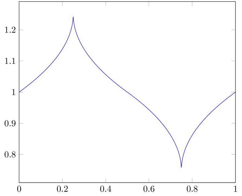
Figure 4: Marginal density $f_{k}(x)$ used in the simulated copula model.

The smoothness of this density is determined by the square root, which has Hölder smoothness $1/2$. The right panel of Figure 4 displays the graph for $d=2.$ This marginal density is appealing as it has a closed-form expression for the density and the c.d.f. The dependency on $d$ of the marginals is to ensure that the marginal densities remain between $1-1/d$ and $1+1/d$ in order to prevent numerical instability. Since the Farlie-Gumbel-Morgenstern copula is infinitely smooth, we get from Lemma 4.4 that the effective smoothness of the joint density generated from this vine-copula approach is equal to $1/2$ and thus the rate $\phi_{n}$ in Theorem 3.4 becomes $n^{-1/2},$ up to $\log(n)$-factors.

5.3 Neural network training setup

For both the SD and FD method and for all training samples, we train $50$ neural networks with width vector $\mathbf{p}=(d,\lceil{(2n)^{1/2}}\rceil,\lceil{(2n)^{1/2}}\rceil,\ldots,\lceil{(2n)^{1/2}}\rceil,1)$ and depth $L=\lceil{\log_{2}(2n)}\rceil$. Since the derived convergence rate of the two-stage neural network estimator is $\phi_{n}=n^{\eta^{\prime}-1/2}$ for the (NBm), (NBs), (BTm) and (BTs) settings and $\phi_{n}=n^{-1/2}$ for the (C) setting, this choice of the network width satisfies the bound in Theorem 3.4. The chosen depth is of the order $\log(n)$ suggested by the theory, but there might be a mismatch regarding the constants in the lower bound of Condition (iii) in Theorem 3.4. Since the proof of this result does not optimize the constants, we find it more appealing to work with the generic choice $L=\lceil{\log_{2}(2n)}\rceil$ in the simulations. Furthermore, Theorem 3.4 imposes a sparsity condition on the networks as well as a condition on the maximum norm of the parameters. In the simulation study we use $\ell_{2}$-penalization on the weight matrices and the Glorot uniform initialization [21] to ensure that the parameter values do not become too large. Although these methods do not provide a hard guarantee that the condition on the maximum norm is satisfied, they work reasonably well in practice and the number of learned network parameters that are larger in absolute value than one is small compared to the total number of network parameters. We use pruning (using the TensorFlow model optimization package) to enforce sparsity. The fraction of zero network parameters is chosen as $1-2m\log(m)\phi_{m}/p$, with $p$ the total number of network parameters and $m=2n$ for the FD method and $m=n$ for the SD method.

The source code is available on GitHub [10].

5.4 Simulation Results

We compare the performance of all the methods on $10^{6}$ test samples. This sample is only used for computing the test error and none of the methods has access to the test samples during training. Figures 5-7 report the test errors for the five different settings.

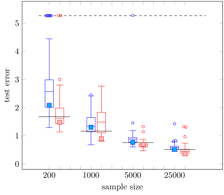
(a) NBs, dimension 4

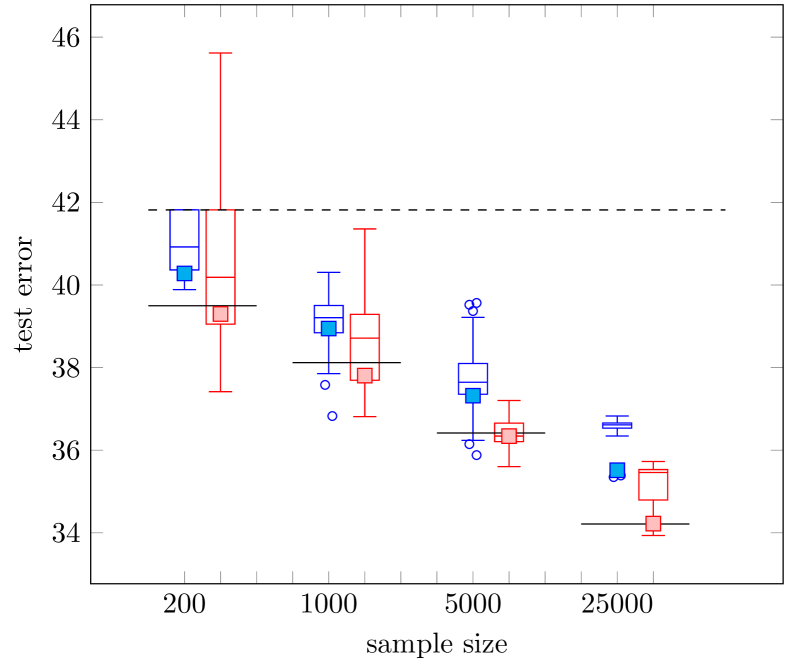
(b) NBs, dimension 12

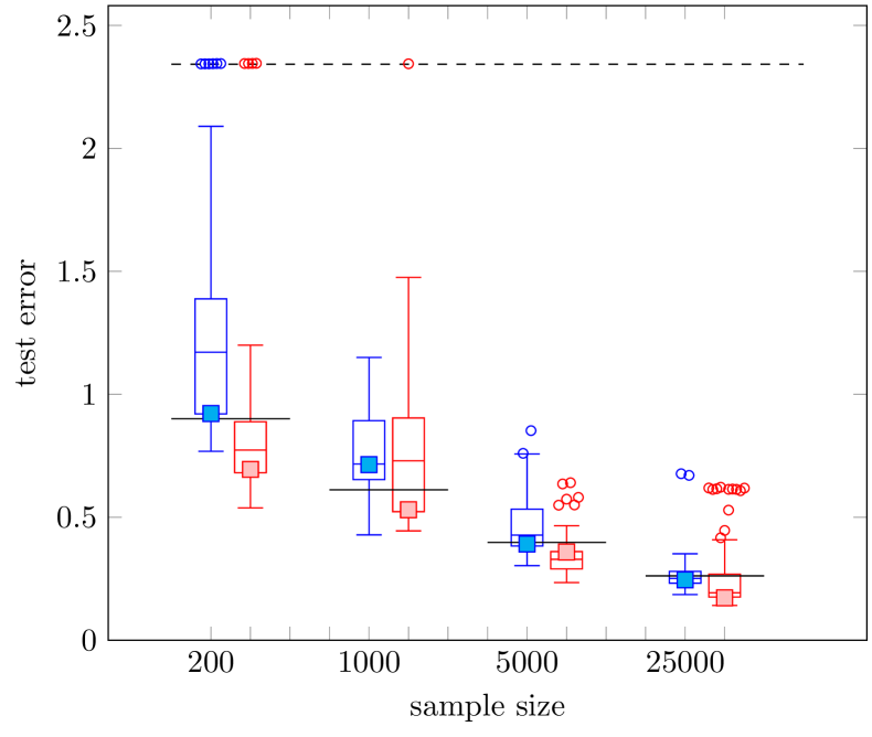
(c) NBm, dimension 4

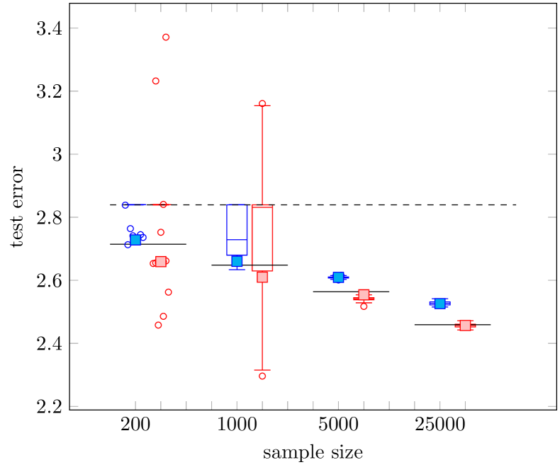
(d) NBm, dimension 12

Figure 5: Test errors for the naive Bayes model. SD in blue, FD in red, KDE black bars. The test error of the network with the lowest training error is indicated by the filled square. The black dashed line is the test error of the zero function. Notice that in the individual plots, the $y$-axis has different starting points.

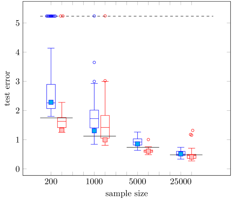
(a) BTs, dimension 4

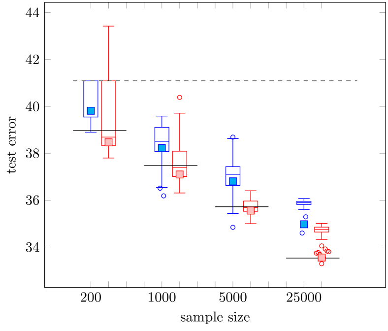
(b) BTs, dimension 12

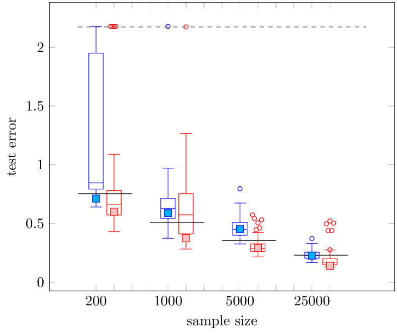
(c) BTm, dimension 4

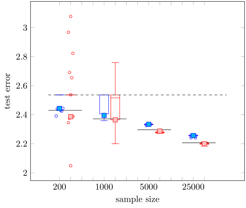
(d) BTm, dimension 12

Figure 6: Test errors for the Bayesian network model. SD in blue, FD in red, KDE black bars. The test error of the network with the lowest training error is indicated by the filled square The black dashed line is the test error of the zero function. Notice that in the individual plots, the $y$-axis has different starting points.

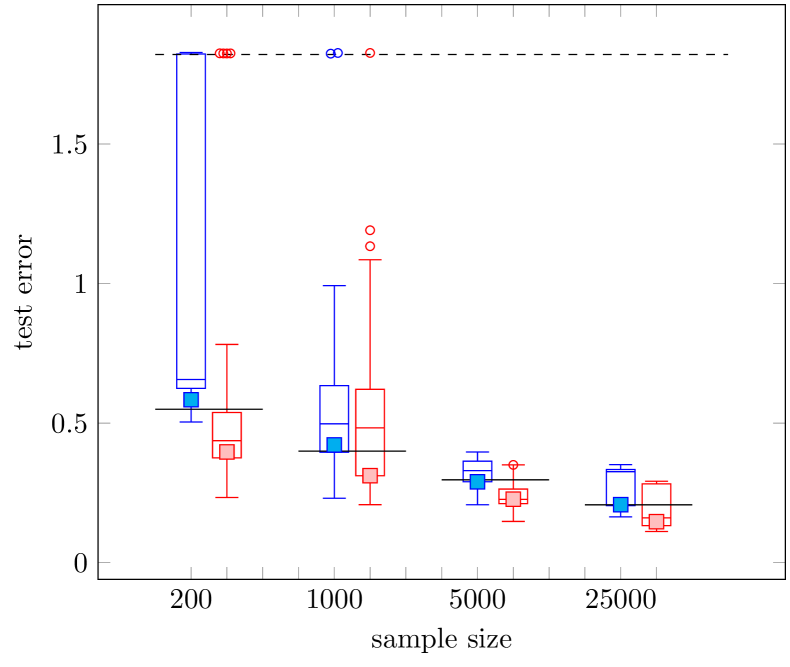
(a) Copula, dimension 4

(b) Copula, dimension 12

Figure 7: Test errors for the Copula model. SD in blue, FD in red, KDE black bars. The test error of the network with the lowest training error is indicated by the filled square. The black dashed line is the test error of the zero function. Notice that in the individual plots, the $y$-axis has different starting points.

For the smaller sample sizes there is in all models some degree of concentration of the test errors of the trained networks around the value of the test error for the zero function. The theory claims that among the sparsely connected networks that satisfy all the imposed conditions, the one with small training error should perform particularly well. To see whether there is an effect, we mark for every simulation setting the test error of the network with the smallest training error by a filled square.

To further investigate the relation between training error and test error, we plot for the (NBs) model in dimension four (Figure 8) and twelve (Figure 9) the training error versus the test error of all networks, for both the SD and FD method and for all the four considered sample sizes. The linear line displaying the least squares regression fit has positive slope, except for the SD method with sample size 1000 (in both dimensions four and twelve).

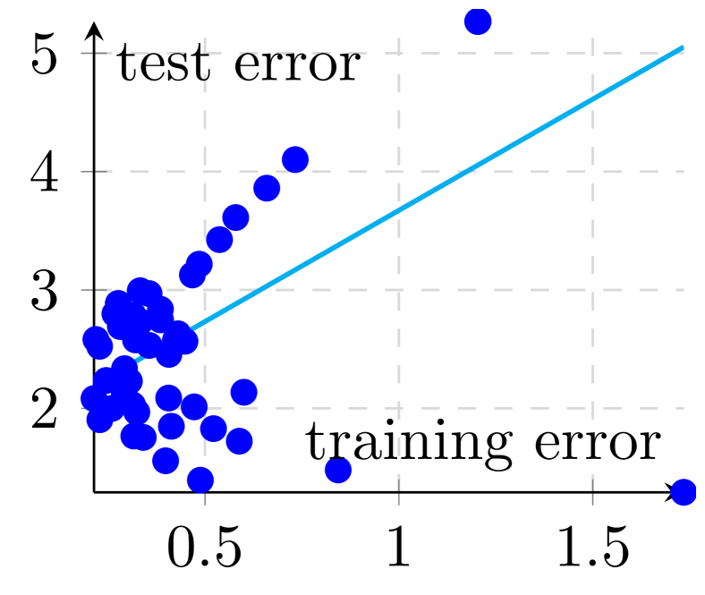
(a) SD method, sample size $200$

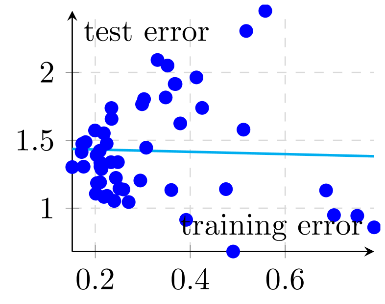
(b) SD method, sample size $1000$

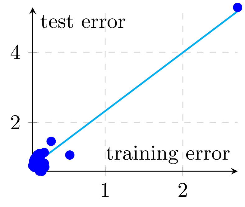
(c) SD method, sample size $5000$

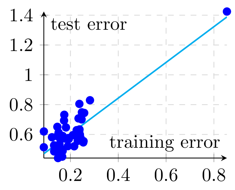
(d) SD method, sample size $25000$

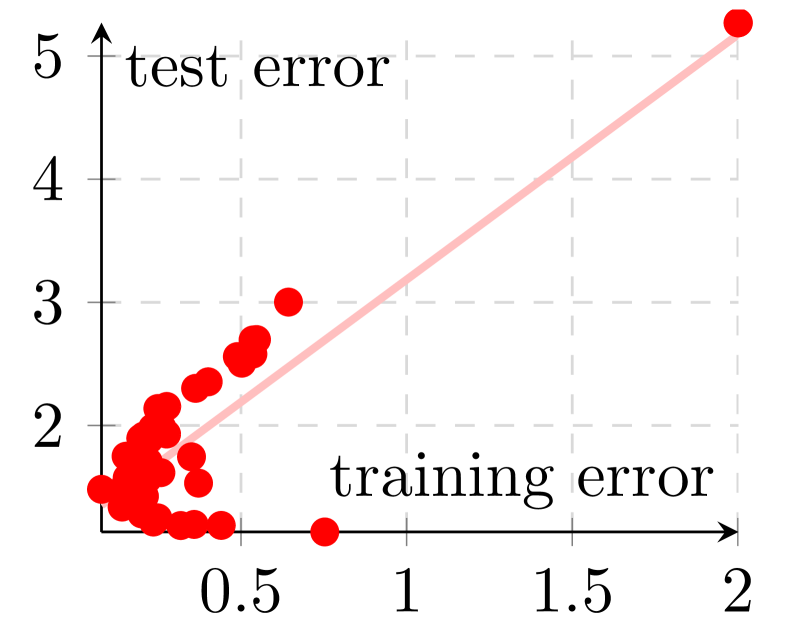
(e) FD method, sample size $200$

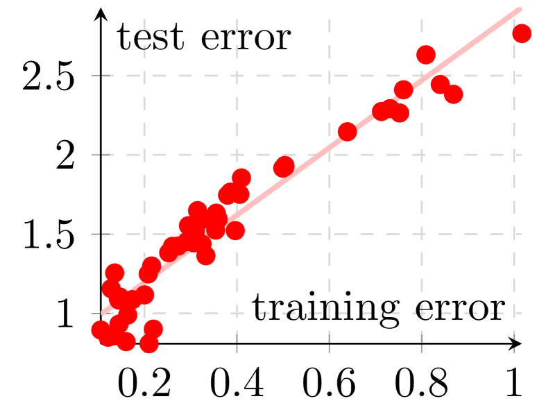
(f) FD method, sample size $1000$

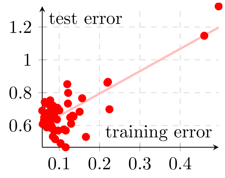
(g) FD method, sample size $5000$

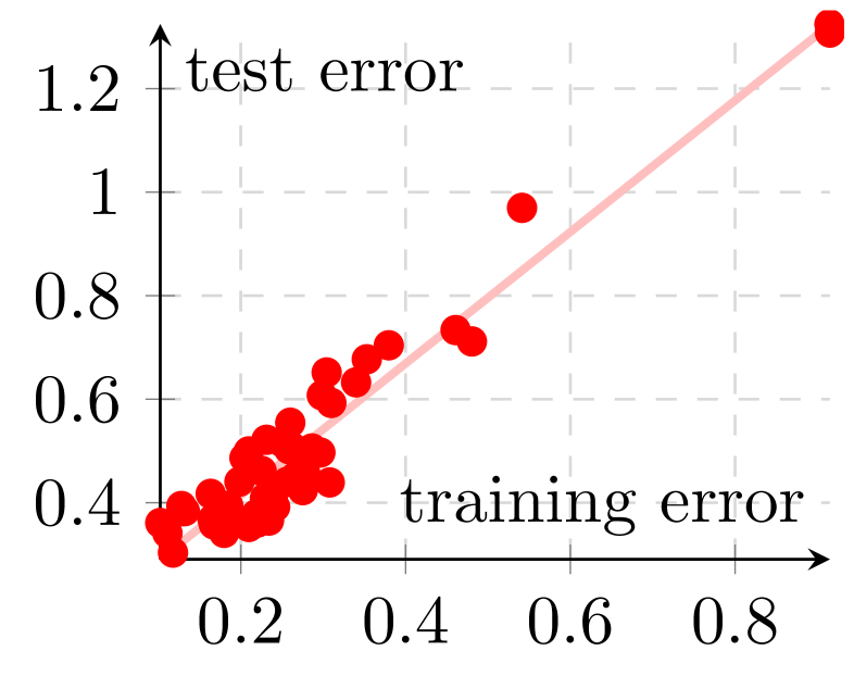
(h) FD method, sample size $25000$

Figure 8: Scatterplot of the training error versus the test error for the (NBs) model in 4 dimensions. The line shows the linear least squares regression fit.

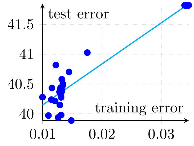
(a) SD method, sample size $200$

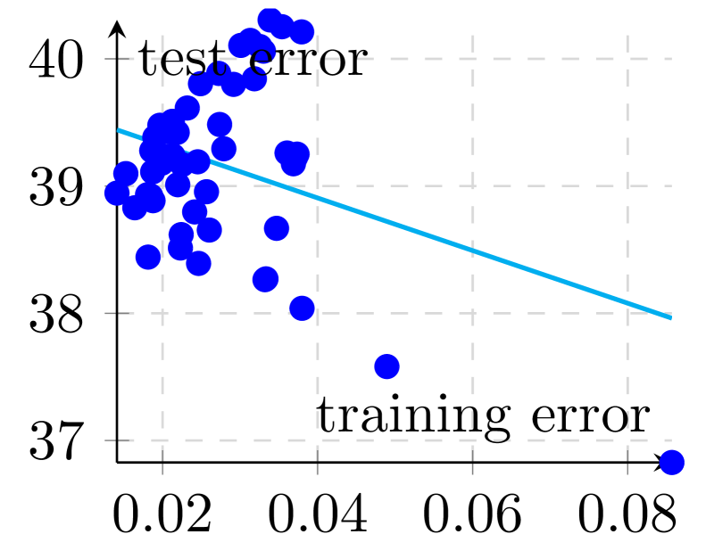
(b) SD method, sample size $1000$

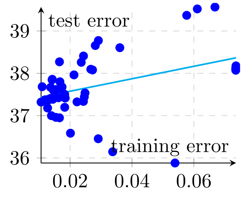
(c) SD method, sample size $5000$

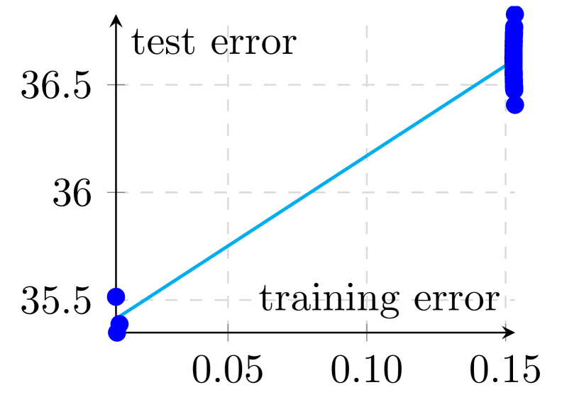
(d) SD method, sample size $25000$

(e) FD method, sample size $200$

(f) FD method, sample size $1000$

(g) FD method, sample size $5000$

(h) FD method, sample size $25000$

Figure 9: Scatterplot of the training error versus the test error for the (NBs) model in 12 dimensions. The line shows the linear least squares regression fit.

To estimate the joint density depending on four variables, the FD method achieves the lowest test error among the three methods for all sample sizes. The test error of the SD method is higher but decreases faster than the test errors of the FD and KDE method. For density estimation on $[0,1]^{12},$ the picture is less clear. The FD method obtains the best error for most densities and sample sizes, but the KDE method achieves an error comparable or even better than the best FD network at training time for some of the sample sizes.

Summarizing the simulation study, we see that for small sample sizes the FD method performs in general better than multivariate kernel density estimation. The fact that networks with small training errors (filled squares in the plots) perform particularly well suggests that the performance of the FD method could be further increased by fitting much larger networks. Although sample splitting makes the theory tractable, we do not advise to use it in practice. While the idea to transform an unsupervised learning problem into a supervised learning problem and using supervised learning methods is appealing, we feel that considerable future effort is required to transform this into stable and efficient algorithms.

6 Proofs for Section 3

Proof of Lemma 3.2.

For all $x\geq 0,$ we have $x<1+x\leq e^{x}$ and thus $\log n/n<1$ as well as $0<u_{n}:=2(\log n/n)^{1/d}<2$ for all $n>1.$ For all $y>0,$ one can find an integer $r$ such that $y/2\leq 2^{r}\leq y.$ If $y<2,$ we must have $r\leq 0.$ Thus, there exists $s\leq 0$ such that $u_{n}/2\leq 2^{s}\leq u_{n}.$ Set $h_{n}=2^{s}.$ Since $s\leq 0,$ we must have $h_{n}^{-1}=2^{-s},$ which is an integer. ∎

6.1 Proof of Theorem 3.1

The response variables $Y_{i}$ in the regression model (2.3) are identically distributed, but they are not jointly independent as they all depend through the kernel density estimator on the subsample $(\mathbf{X}^{\prime}_{\ell})_{\ell=1}^{n}.$

To deal with the dependence induced by the kernel density estimator, we partition the hypercube $[0,1]^{d}$ into $h_{n}^{-d}$ hypercubes with sidelength $h_{n}^{-1}.$ By construction $h_{n}^{-1}$ is an integer and therefore no boundary issues arise. The centers of these $h_{n}^{-d}$ hypercubes are given by the vectors $h_{n}(k_{1}-1/2,k_{2}-1/2,\ldots,k_{d}-1/2)^{\top}\in[0,1]^{d}$ with $k_{1},k_{2},\ldots,k_{d}\in\{1,\ldots,h_{n}^{-1}\}.$ By numbering these points (the specific numbering of the points is irrelevant), we assign to each center an index in $\mathcal{J}:=\{1,\ldots,h_{n}^{-d}\}.$ The $j$-th bin $\mathcal{B}_{j}$ is then the $|\cdot|_{\infty}$-norm ball of radius $h_{n}/2$ around the $j$-th center $C(\mathcal{B}_{j})$ in this index set. To avoid that boundary points are in two bins, we include a boundary point only if is not already included in a bin with smaller index in the ordering induced by $\mathcal{J}$. This construction gives a partition of $[0,1]^{d}.$ As each bin is a hypercube with sidelength $h_{n}$, the Lebesgue measure is $h_{n}^{d}$ (in $\mathbb{R}^{d}$). The neighborhood of a bin $\mathcal{B}_{j},$ denoted by $NB(\mathcal{B}_{j}),$ are all bins whose centers are at most $|\cdot|_{\infty}$-distance away from the center of $\mathcal{B}_{j}$, in other words,

$$NB(\mathcal{B}_{j})=\{\widetilde{j}:|C(\mathcal{B}_{j})-C(\mathcal{B}_{\widetilde{j}})|_{\infty}\leq h_{n}\}.$$ (6.1)

(In two dimensions this neighborhood is also known as the Moore neighborhood).

We further subdivide the bins into equivalence classes. The hypercube $[0,3h_{n}]^{d}$ contains exactly $3^{d}$ bins. Denote by $(j_{s})_{s=1}^{3^{d}}$ the indices of these bins and define the index set $\mathcal{J}_{s}\subset\mathcal{J}$ by

$$\mathcal{J}_{s}:=\Big{\{}j\in\mathcal{J}:|C(\mathcal{B}_{j})-C(\mathcal{B}_{j_{s}})|_{\infty}=m3h_{n}\text{ for some integer m }\Big{\}}.$$

By construction, the sets $\mathcal{J}_{s}$ are mutually disjoint and $\bigcup_{s}\mathcal{J}_{s}=\mathcal{J}.$

Fix a $j\in\mathcal{J}.$ Since the kernel $K$ in the kernel density estimator has bandwidth $h_{n}$ and support contained in $[-1,1]$, the point estimator $\widehat{f}_{\operatorname{KDE}}(\mathbf{x})$ only depends on the data points from the kernel data set $(\mathbf{X}^{\prime}_{\ell})_{\ell=1}^{n}$ that are in $NB(\mathcal{B}_{j}).$

More generally, for two different indices $j,\widetilde{j}\in\mathcal{J}_{s}$, $j\neq\widetilde{j}$ and points $\mathbf{x}_{1}\in\mathcal{B}_{j}$, $\mathbf{x}_{2}\in\mathcal{B}_{\widetilde{j}},$ the point estimators $\widehat{f}_{\operatorname{KDE}}(\mathbf{x}_{1})$ and $\widehat{f}_{\operatorname{KDE}}(\mathbf{x}_{2})$ depend on $\{\mathbf{X}^{\prime}_{\ell}:\mathbf{X}^{\prime}_{\ell}\in NB(\mathcal{B}_{j}),\ell=1,\ldots,n\}$ and $\{\mathbf{X}^{\prime}_{\ell}:\mathbf{X}^{\prime}_{\ell}\in NB(\mathcal{B}_{\widetilde{j}}),\ell=1,\ldots,n\},$ respectively. The latter two sets are dependent if $n$ is fixed (knowing that a data point is in one of the bins means that there can be at most $n-1$ in any of the other bins). If we instead assume that the sample size of the data set $(\mathbf{X}_{\ell}^{\prime})_{\ell=1}^{n}$ is not $n$ but $\mathcal{M}$ with $\mathcal{M}\sim\operatorname{Poisson}(n)$, then $\{\mathbf{X}^{\prime}_{\ell}:\mathbf{X}^{\prime}_{\ell}\in A,\ell=1,\ldots,N\}$ and $\{\mathbf{X}^{\prime}_{\ell}:\mathbf{X}^{\prime}_{\ell}\in B,\ell=1,\ldots,N\}$ are independent, whenever $A$ and $B$ are disjoint sets. Using Poisson point process theory, we also show in the proof of Lemma 6.2 that $\widehat{f}_{\operatorname{KDE}}(\mathbf{x}_{1})$ and $\widehat{f}_{\operatorname{KDE}}(\mathbf{x}_{2})$ are independent.

The previously described strategy is known as Poissonization, cf. [51] Section 3.5.2., [19], [16] Section 8.3. In particular, we use the following inequality

Lemma 6.1.

For any function $h$ and any measurable set $A$,

$$\mathbb{P}\bigg{(}\sum_{i=1}^{n}h(\mathbf{X}_{i}^{\prime})\in A\bigg{)}\leq\sqrt{2e\pi n}\,\mathbb{P}\bigg{(}\sum_{i=1}^{\mathcal{M}}h(\mathbf{X}_{i}^{\prime})\in A\bigg{)}.$$

Proof of Lemma 6.1.

We have

$$\mathbb{P}\bigg{(}\sum_{i=1}^{n}h(\mathbf{X}_{i}^{\prime})\in A\bigg{)} =\mathbb{P}\bigg{(}\sum_{i=1}^{\mathcal{M}}h(\mathbf{X}_{i}^{\prime})\in A\,\bigg{|}\,\mathcal{M}=n\bigg{)}\leq\frac{\mathbb{P}\big{(}\sum_{i=1}^{\mathcal{M}}h(\mathbf{X}_{i}^{\prime})\in A\big{)}}{\mathbb{P}(\mathcal{M}=n)}.$$

Since $\mathcal{M}$ is a $\operatorname{Poisson}(n)$ random variable we have that $\mathbb{P}(\mathcal{M}=n)=n^{n}e^{-n}/n!.$ By Stirling’s formula, see for example [45], $n!\leq\sqrt{2\pi n}(n/e)^{n}e^{1/(12n)}\leq\sqrt{2e\pi n}(n/e)^{n}$ and $1/\mathbb{P}(\mathcal{M}=n)\leq\sqrt{2e\pi n}.$ ∎

While Poissonization removes dependence, the factor $\sqrt{2e\pi n}$ arises in the bounds.

Proving oracle inequalities for the risk $R(\widetilde{f},f_{0}):=\mathbb{E}_{f_{0},\mathbf{X}}[(\widetilde{f}(\mathbf{X})-f_{0}(\mathbf{X}))^{2}]$ in the standard i.i.d. setting typically first shows an oracle inequality for the empirical risk $\widehat{R}_{n}(\widehat{f},f_{0})$ as

$$\widehat{R}_{n}(\widehat{f},f_{0}):=\mathbb{E}_{f_{0}}\left[\frac{1}{n}\sum_{i=1}^{n}\big{(}\widehat{f}(\mathbf{X}_{i})-f_{0}(\mathbf{X}_{i})\big{)}^{2}\right].$$

Here empirical refers to the fact that the estimator $\widehat{f}$ is evaluated at the data points $\mathbf{X}_{1},\ldots,\mathbf{X}_{n}.$ The derivation of an oracle inequality for the empirical risk can be further subdivided into several steps. The bound below refers to the step where our setting and the i.i.d. case differ the most. The proof relies heavily on the construction of the bins above combined with Poissonization.

Lemma 6.2.

For any estimator $\widehat{f}$ as in Theorem 3.1, any fixed $f\in\mathcal{F}$ and $\log^{2}(n)\log(\mathcal{N}_{\mathcal{F}}(\delta))\leq n,$ it holds that

$$\bigg{|}\mathbb{E}_{f_{0}}\bigg{[}\frac{2}{n}\sum_{i=1}^{n}\epsilon_{i}(\widehat{f}(\mathbf{X}_{i})-f(\mathbf{X}_{i}))\bigg{]}\bigg{|}$$

$$\leq 2^{d+6}14e^{2}\|K\|_{\infty}^{2d}F^{3}3^{\frac{7d}{2}}\bigg{(}\sqrt{\widehat{R}_{n}(\widehat{f},f_{0})}\log(n)\sqrt{\frac{\log(\mathcal{N}_{\mathcal{F}}(\delta))}{n}}+\log(n)\frac{\log(\mathcal{N}_{\mathcal{F}}(\delta))}{n}+\delta\bigg{)}$$

$$\quad+\frac{65F^{2}2^{d}\|K\|_{\infty}^{d}}{n}+8h_{n}^{2\beta}F^{2}d^{2\beta}\|K\|_{\infty}^{2d}+\frac{\mathbb{E}_{\mathbf{X}}[(f_{0}(\mathbf{X})-f(\mathbf{X}))^{2}]}{4}+\frac{\widehat{R}_{n}(\widehat{f},f_{0})}{4}.$$

With this lemma in place, we can prove the following bound on the empirical risk. This is similar to step (III) in the oracle inequality of Lemma 4 in [46].

Proposition 6.3.

For any estimator $\widehat{f}$ as in Theorem 3.1, any fixed $f\in\mathcal{F}$ and $\log^{2}(n)\log(\mathcal{N}_{\mathcal{F}}(\delta))\leq n,$

$$\widehat{R}_{n}(\widehat{f},f_{0}) \leq\delta 2^{d+6}38e^{2}\|K\|_{\infty}^{2d}F^{3}3^{\frac{9d}{2}}$$

$$+\frac{10}{3}\mathbb{E}_{\mathbf{X}}\left[(f(\mathbf{X})-f_{0}(\mathbf{X}))^{2}\right]+(1+\epsilon)\frac{4}{3}\Delta_{n}(\widehat{f},f_{0})$$

$$+2^{d+6}38e^{2}\|K\|_{\infty}^{2d}F^{3}3^{\frac{7d}{2}}\log(n)\frac{\log(\mathcal{N}_{\mathcal{F}}(\delta))}{n}$$

$$+\frac{174F^{2}2^{d}\|K\|_{\infty}^{d}}{n}+22h_{n}^{2\beta}F^{2}d^{2\beta}\|K\|_{\infty}^{2d}$$

$$+4^{d+7}19^{2}e^{4}\|K\|_{\infty}^{4d}F^{6}3^{7d}\log^{2}(n)\frac{\log(\mathcal{N}_{\mathcal{F}}(\delta))}{n}.$$

We now have all ingredients to finish the proof of Theorem 3.1.

Proof of Theorem 3.1.

If $\log^{2}(n)\log(\mathcal{N}_{\mathcal{F}}(\delta))\geq n$, the statement follows with $C_{1}=4F^{2}$ by observing that $R(\widehat{f},f_{0})\leq 4F^{2}.$

It remains to consider the case $\log^{2}(n)\log(\mathcal{N}_{\mathcal{F}}(\delta))\leq n$. Lemma 4, Part (I) in [46] states that for any $\epsilon\in(0,1],$

$$(1-\epsilon)\widehat{R}_{n}(\widehat{f},f_{0})-\frac{F^{2}}{n\epsilon}\Big{(}15\log\big{(}\mathcal{N}_{\mathcal{F}}(\delta)\big{)}+75\Big{)}-26\delta F$$ (6.2)

$$\leq R(\widehat{f},f_{0})\leq(1+\epsilon)\bigg{(}\widehat{R}_{n}(\widehat{f},f_{0})+(1+\epsilon)\frac{F^{2}}{n\epsilon}\Big{(}12\log(\mathcal{N}_{\mathcal{F}}(\delta))+70\Big{)}+26\delta F\bigg{)}.$$

This lemma for the standard nonparametric regression problem relates the risk to its empirical counterpart. The inequality and its proof only depend on the $\mathbf{X}_{i}$ and on the function class $\mathcal{F}$, not on the noise or the response variables $Y_{i}.$ Since in our regression model (2.3) the variables $\mathbf{X}_{i}$ are i.i.d. (the dependence is induced by the response variables $Y_{i}$ and $\epsilon_{i}$), this inequality is still valid.

Substituting the bound on $\widehat{R}_{n}(\widehat{f},f_{0})$ from Proposition 6.3 in (6.2), choosing $f$ to be a minimizer over $\mathcal{F}$ of $\mathbb{E}_{\mathbf{X}}\left[(f(\mathbf{X})-f_{0}(\mathbf{X}))^{2}\right]$, the fact that $h_{n}\leq 2(\log(n)/n)^{1/d}$, and replacing the explicit constants by $C_{1},C_{2},C_{3}$ yields the result. ∎

6.2 Proof of Theorem 3.4

The following lemma provides a bound on the covering entropy.

Lemma 6.4 (Lemma 5 combined with Remark 1 of [46]).

For any $\delta>0$

$$\log\big{(}\mathcal{N}_{\mathcal{F}(L,\mathbf{p},s,\infty)}(\delta)\big{)}\leq(s+1)\log\left(2^{2L+5}\delta^{-1}(L+1)p_{0}^{2}p_{L+1}^{2}s^{2L}\right).$$

The proof of Theorem 1 in [46] derives the following bound for the approximation error for function approximation in the function class $\mathcal{G}(q,\mathbf{d},\mathbf{t},\bm{\alpha},Q^{\prime})$ by sparsely connected deep ReLU networks.

Theorem 6.5.

For every function $g\in\mathcal{G}(q,\mathbf{d},\mathbf{t},\bm{\alpha},Q^{\prime})$ and whenever

• $\sum_{i=1}^{q}\log_{2}(4t_{i}\vee 4\alpha_{i})\log_{2}(n)\leq L\lesssim n\phi_{n},$

• $n\phi_{n}\lesssim\min_{i=1,\ldots,L}p_{i},$

• $s\asymp n\phi_{n}\log(n),$

• $F\geq\max\{Q^{\prime},1\},$

then there exists a neural network $H\in\mathcal{F}(L,\mathbf{p},s,F)$ and a constant $C_{8}$ only depending on $q,\mathbf{d},\mathbf{t},\bm{\alpha},F$ and the implicit constants in (i), (ii) and (iii), such that

$$\|g-H\|_{\infty}^{2}\leq C_{8}\phi_{n}.$$

We now have all the necessary ingredients to prove Theorem 3.4

Proof of Theorem 3.4.

Apply the general oracle inequality in Theorem 3.1 with the choice $\delta=n^{-1}$ to the neural network class $\mathcal{F}(L,\mathbf{p},s,F)$ with parameter constraints as in the statement of the theorem. For the approximation error in the oracle inequality, we use Theorem 6.5 and for the covering entropy the bound from Lemma 6.4. This yields the result. ∎

7 Proofs for Section 4

Lemma 7.1.

Let $m$ be a positive integer and $Q>0.$ Then $f:[-Q,Q]^{m}\rightarrow\mathbb{R}$: $f(\mathbf{x}):=\prod_{i=1}^{m}x_{i}$ is in $C^{\gamma}_{m}([-Q,Q]^{m},(Q+1)^{m}),$ for all $\gamma\geq m+1$.

Proof.

Observe that $|\partial^{0}f(\mathbf{x})|=|f(\mathbf{x})|\leq Q^{m}$, $\partial_{x_{j}}f(\mathbf{x})=\prod_{i=1,i\neq j}^{m}x_{i}$ and $\partial_{x_{j}}\partial_{x_{j}}f=0,$ for $i=1,\ldots,m.$ This means that for all $\bm{\alpha}\in\mathbb{Z}^{m}_{\geq 0}$ it holds that $\partial^{\bm{\alpha}}f=0$ if $\alpha_{j}\geq 2$ for some $j\in\{1,\ldots,m]$. Rephrased, $\partial^{\bm{\alpha}}f\neq 0$ if and only if $\bm{\alpha}\in\{0,1\}^{m}$. Furthermore for $\bm{\alpha}\in\{0,1\}^{m},$ $|\partial^{\bm{\alpha}}f(\mathbf{x})|=|\prod_{i:\alpha_{i}=0}x_{i}|\leq Q^{m-|\bm{\alpha}|_{0}},$ where $|\cdot|_{0}$ denotes the counting norm. There are $\binom{m}{m-|\bm{\alpha}|_{0}}$ ways to distribute $m-|\bm{\alpha}|_{0}$ zeros over a vector of length $m$. So for $\gamma\geq m+1,$ we get by the binomial theorem

$$\sum_{\bm{\alpha}:|\bm{\alpha}|_{1}<\gamma}\|\partial^{\bm{\alpha}}f\|_{\infty}\leq\sum_{k=0}^{m}\binom{m}{k}Q^{k}=(Q+1)^{m}.$$

If $|\bm{\alpha}|_{1}>m,$ then there exists at least one $j$ such that $\alpha_{j}\geq 2$ and thus we have that $\partial^{\bm{\alpha}}f=0$ in this case. In the case that $|\bm{\alpha}|_{1}=m$, then either there exists a $j$ such that $\alpha_{j}\geq 2$, so $\partial^{\bm{\alpha}}f=0$, or $\bm{\alpha}$ is the vector with only ones, in which case $\partial^{\bm{\alpha}}f=1$. Hence, $\gamma\geq m+1$ yields

$$\sum_{\bm{\alpha}:|\bm{\alpha}|_{1}=\lfloor{\gamma}\rfloor}\sup_{\mathbf{x},\mathbf{y}\in\mathcal{D},\mathbf{x}\neq\mathbf{y}}\frac{|\partial^{\bm{\alpha}}f(\mathbf{x})-\partial^{\bm{\alpha}}f(\mathbf{y})|}{|\mathbf{x}-\mathbf{y}|_{\infty}^{\gamma-\lfloor{\gamma}\rfloor}}=0.$$

Together with the definition the Hölder ball, (3.1), the statement follows. ∎

Proof of Lemma 4.1.

The function $g_{0}=(g_{0,1},\ldots,g_{0,|\mathcal{R}|})$ is given by $g_{0,I}=\psi_{I}$ for all $I\in\mathcal{R}$. From $\psi_{I}\in C_{r_{I}}^{\gamma}([0,1]^{r_{I}},Q)$ and $|I|\leq r$ it follows that $t_{0}=r$ and $\alpha_{0}=\gamma.$ The function $g_{1}(u_{1},\ldots,u_{|\mathcal{R}|})=\prod_{I\in\mathcal{R}}u_{I}$ is the product of $|\mathcal{R}|$ different terms in $[-Q,Q]^{|\mathcal{R}|}.$ Applying Lemma 7.1 yields $g_{1}\in\mathcal{C}^{\zeta}_{|\mathcal{R}|}([-Q,Q]^{|\mathcal{R}|},(Q+1)^{|\mathcal{R}|})$ for all $\gamma\geq|\mathcal{R}|+1.$ So $t_{1}=|\mathcal{R}|$ and $\alpha_{1}$ is arbitrarily large. ∎

Proof of Lemma 4.2.

We argue by contradiction. Let $j$ be the index of the marginal densities that is at most $\alpha$-Hölder smooth. Denote the Hölder smoothness of $f$ by $\beta$ and suppose that $\beta>\alpha.$ Then there exists a constant $Q$ such that $f\in C^{\beta}_{d}([0,1]^{d},Q).$ By the chain rule and because $f$ is $\beta$-Hölder smooth it holds that

$$\frac{\partial^{k}}{\partial x_{j}^{k}}f(\mathbf{x})=\bigg{(}\prod_{i\neq j}f_{i}(x_{i})\bigg{)}\frac{\partial^{k}}{\partial x_{j}^{k}}f_{j}(x_{j})$$ (7.1)

for all $k=0,1,\ldots,\lfloor{\beta}\rfloor$. Since $\prod_{i\neq j}f_{i}$ is a density on $[0,1]^{d-1},$ it is nonnegative and there exists a $\widetilde{\mathbf{x}}_{-j}=(\widetilde{x}_{1},\ldots,\widetilde{x}_{j-1},\widetilde{x}_{j+1},\ldots,\widetilde{x}_{d})\in[0,1]^{d-1}$ such that $\prod_{i\neq j}f_{i}(\widetilde{x}_{i})=C>0.$ Since $f_{j}$ only depends on $x_{j}$ and $f$ is $\beta$-Hölder smooth, for any $k=0,1,,\ldots,\lfloor{\beta}\rfloor,$

$$\frac{Q}{C}\geq\frac{1}{C}\bigg{\|}\bigg{(}\prod_{i\neq j}f_{i}\bigg{)}\frac{\partial^{k}}{\partial x_{j}^{k}}f_{j}\bigg{\|}_{L^{\infty}([0,1]^{d})}\geq\frac{\prod_{i\neq j}f_{i}(\widetilde{x}_{i})}{C}\left\|\frac{\partial^{k}}{\partial x_{j}^{k}}f_{j}\right\|_{L^{\infty}([0,1])}=\left\|\frac{\partial^{k}}{\partial x_{j}^{k}}f_{j}\right\|_{L^{\infty}([0,1])}.$$ (7.2)

Similarly, by the $\beta$-Hölder smoothness of $f$ and (7.1),

$$\begin{split}\frac{Q}{C}&\geq\frac{1}{C}\sup_{\mathbf{x},\mathbf{y}\in[0,1]^{d},\mathbf{x}\neq\mathbf{y}}\frac{\left|\frac{\partial^{\lfloor{\beta}\rfloor}}{\partial x_{j}^{\lfloor{\beta}\rfloor}}f(\mathbf{x})-\frac{\partial^{\lfloor{\beta}\rfloor}}{\partial x_{j}^{\lfloor{\beta}\rfloor}}f(\mathbf{y})\right|}{|\mathbf{x}-\mathbf{y}|_{\infty}^{\beta-\lfloor{\beta}\rfloor}}\\ &\geq\frac{\prod_{i\neq j}f_{i}(\widetilde{x_{i}})}{C}\sup_{x,y\in[0,1],x\neq y}\frac{\left|\frac{\partial^{\lfloor{\beta}\rfloor}}{\partial x_{j}^{\lfloor{\beta}\rfloor}}f_{j}(x)-\frac{\partial^{\lfloor{\beta}\rfloor}}{\partial x_{j}^{\lfloor{\beta}\rfloor}}f_{j}(y)\right|}{|x-y|^{\beta-\lfloor{\beta}\rfloor}}.\end{split}$$ (7.3)

From (7.2) and (7.3) it follows that $f_{j}\in C^{\beta}_{1}([0,1],(\lfloor{\beta}\rfloor+1)Q/C).$ Since $\beta>\alpha,$ this contradicts the condition that $f_{j}$ was at most $\alpha$-Hölder smooth. Therefore, $\beta\leq\alpha.$ ∎

Proof of Lemma 4.3.

The function $g_{0}=(g_{0,1},\ldots,g_{0,2d})$ is given by $g_{0,i}(x_{i})=f_{i}(x_{i})$ for $i=1,\ldots,d$ and $g_{0,i}(x_{i-d})=F_{i-d}(x_{i-d})$ for $i=d+1,\ldots,2d.$ Each of these functions is univariate, so $t_{0}=1.$ Since $F_{i-d}$ is the c.d.f. of $f_{i},$ it holds that $F_{i-d}\in C_{1}^{\gamma_{i}+1}([0,1],Q_{i}+1)$. Thus the function $g_{0,i}$ with the smallest Hölder smoothness has to correspond to one of the functions $f_{i}$ and $\alpha_{0}=\min_{i=1,\ldots,d}\gamma_{i}$. The function $g_{1}=(g_{1,1},\ldots,g_{1,d+1})$ satisfies $g_{1,i}(y_{i})=y_{i}$ (the identity function) for $i=1,\ldots,d$ and $g_{1,d+1}(\mathbf{v})=c(v_{1},\ldots,v_{d})$, so $t_{1}=d$. For $i=1,\ldots,d$ the domain of $g_{1,i}$ is $[0,\|f_{i}\|_{\infty}]\subseteq[0,Q_{i}]$, so $g_{1,i}\in C^{\gamma}_{1}([0,Q_{i}],Q_{i}+1),$ for all $\gamma\geq 2.$ This means the Hölder smoothness of $g_{1,i}$ can be taken arbitrarily large, that consequently $g_{1,d+1}$, corresponding to the copula $c$, has the smallest Hölder smoothness among the component functions of $g_{1},$ and thus $\alpha_{1}=\gamma_{c}$. Set $Q:=Q_{c}\vee(\max_{i=1,\ldots,d}Q_{i})$, then $g_{2}(u,y_{1},\ldots,y_{d})=u\prod_{i=1}^{d}y_{i}$ is the product of $d+1$ different factors in $[-Q,Q]^{d+1}$. Applying Lemma 7.1 yields $g_{2}\in C^{\gamma}_{d+1}([-Q,Q]^{d+1},(Q+1)^{d+1})$ for all $\gamma\geq d+2.$ So $t_{2}=d+1$ and the smoothness index $\alpha_{2}$ can be taken to be arbitrarily large.∎

Proof of Lemma 4.4.

The function $g_{0}=(g_{0,1},\ldots,g_{0,2d})$ is given by $g_{0,i}(x_{i})=f_{i}(x_{i})$ for $i=1,\ldots,d$ and $g_{0,i}(x_{i-d})=F_{i-d}(x_{i-d})$ for $i=d+1,\ldots,2d$. Since $F_{i-d}$ is the c.d.f. of $f_{i},$ it holds that $F_{i-d}\in C_{1}^{\gamma_{m,i}+1}([0,1],Q_{m,i}+1)$. So $t_{0}=1$ and $\alpha_{0}=\min_{i=1,\ldots,d}\gamma_{m,i}$. The function $g_{1}=(g_{1,1},\ldots,g_{1,d+(d-1)})$ satisfies $g_{1,i}(u_{i})=u_{i}$ (the identity function) for $1=1,\ldots,d$. For $f$ of the form (4.8) it holds that $g_{1,i}(v_{1},v_{2})=c_{1,i+1-d}(v_{1},v_{2})$ for $i=d+1,\ldots,d+(d-1)$ and for $f$ of the form (4.9) we have that $g_{1,i}(v_{1},v_{2})=c_{i-d,i+1-d}(v_{1},v_{2})$ for $i=d+1,\ldots,d+(d-1)$. For $i=1,\ldots,d$ the domain of $g_{1,i}$ is $[0,\|f_{i}\|_{\infty}]\subseteq[0,Q_{m,i}]$, so for $i=1,\ldots,d$ it holds that $g_{1,i}\in C^{\gamma}_{1}([0,Q_{m,i}],Q_{m,i}+1),$ for all $\gamma\geq 2.$ This means the Hölder smoothness of $g_{1,i},$ for $i=1,\ldots,d$, can be taken to be arbitrarily large. So $t_{1}=2$ and $\alpha_{2}=\gamma_{c}.$ Set $Q=(\max_{i=1,\ldots,d}Q_{m,i})\vee Q_{c}.$ The function $g_{2}(u_{1},\ldots,u_{d},y_{1},\ldots,y_{d-1})=\prod_{k=1}^{d}u_{k}\prod_{j=1}^{d-1}y_{j}$ is the product of $2d-1$ terms. Thus by Lemma 7.1 it holds that $g_{2}\in C_{2d-1}^{\gamma}([-K,K]^{2d-1},(Q+1)^{2d-1})$ for all $\gamma\geq 2d$, so $\alpha_{2}$ is arbitrarily large and $t_{2}=2d-1.$ ∎

7.1 Proof of Theorem 4.5

Recall that we work in the density estimation model as defined in Section 2 with mixture density $f_{0}=\sum_{j=1}^{r}a_{j}f_{j}$, where $a_{1},\ldots a_{r}$ are non-negative mixture weights summing up to one, and $f_{j}\in\mathcal{C}_{d}^{\beta_{j}}([0,1]^{d},Q)\cap\mathcal{G}(q_{j},\mathbf{d}_{j},\mathbf{t}_{j},\bm{\alpha}_{j},Q),$ for $i=1,\ldots,r$. Set $\phi_{n}^{\star}=\max_{j=1,\ldots,r}\phi_{n,j}$, where $\phi_{n,j}$ is the rate (3.4) for estimation of $f_{j}$ and set $\beta=\min_{j=1,\ldots,r}\beta_{j}$.

Lemma 7.2 (Approximation of mixtures).

Whenever

• $\max_{j=1,\ldots,r}\sum_{i=1}^{q}\log_{2}(4t_{i,j}\vee 4\alpha_{i,j})\log_{2}(n)\leq L\lesssim n\phi_{n}^{\star},$

• $n\phi_{n}^{\star}\lesssim\min_{i=1,\ldots,L}p_{i},$

• $s\asymp n\phi_{n}^{\star}\log(n),$

• $F\geq\max\{Q,1\},$

then, for $n$ large enough, there exists a network $H\in\mathcal{F}(L,\mathbf{p},s,F)$ and a constant $C_{9}$ only depending on $(q_{j},\mathbf{d}_{j},\mathbf{t}_{j},\bm{\alpha}_{j})_{j=1}^{r},$ $r,F$ and the implicit constants in (i), (ii) and (iii) such that

$$\bigg{\|}\sum_{j=1}^{r}a_{j}f_{j}-H\bigg{\|}_{\infty}^{2}\leq C_{9}\phi_{n}^{\star}.$$

Proof.

For positive constants $c_{L},c_{p},c_{s\ell},c_{su},$ let $L^{\star}$, $\mathbf{p}^{\star}$ and $s^{\star}$ be such that

• $\max_{j=1,\ldots,r}\sum_{i=1}^{q}\log_{2}(4t_{i,j}\vee 4\alpha_{i,j})\log_{2}(n)\leq L^{\star}\leq c_{L}n\phi_{n}^{\star}$

• $n\phi_{n}^{\star}\leq c_{p}\min_{i=1,\ldots,L}p_{i}^{\star}$

• $c_{s\ell}n\phi_{n}^{\star}\log(n)\leq s^{\star}\leq c_{su}n\phi_{n}^{\star}\log(n).$

For $n$ large enough, we have

• $c_{L}n\phi_{n}^{\star}\leq(c_{s\ell}/(2r))n\phi_{n}^{\star}\log(n)$,

• $n\phi_{n}^{\star}>rc_{p}$,

• $\lfloor{c_{L}n\phi_{n,j}}\rfloor\geq\sum_{i=1}^{q}\log_{2}(4t_{i,j}\vee 4\alpha_{i,j})\log_{2}(n)$,

• $(c_{sl}/(4r))n\phi_{n,j}\log(n)\geq 1.$

For $j=1,\ldots,r$ define $L_{j}:=\min\{L^{\star},\lfloor{c_{L}n\phi_{n,j}}\rfloor\}$, $p_{i,j}=\lfloor{p_{i}^{\star}/r}\rfloor$ and $s_{j}=\lfloor{s^{\star}\phi_{n,j}/(2r\phi_{n}^{\star})}\rfloor$. Recall that $\phi_{n}^{\star}=\max_{j=1,\ldots,r}\phi_{n,j}$. Using the definition of $L_{j}$ and (III) yields

$$\sum_{i=1}^{q}\log_{2}(4t_{i,j}\vee 4\alpha_{i,j})\log_{2}(n)\leq L_{j}\leq c_{L}n\phi_{n,j}.$$

Using the definition of $\mathbf{p}_{j}$ we get that

$$n\phi_{n,j}\leq(c_{p}/r)\min_{i=1,\ldots,L}p_{i,j}.$$

From $\lfloor{u}\rfloor\geq u-1$ for all $u\in\mathbb{R}$, the definition of $s_{j},$ and (IV) it follows that

$$(c_{sl}/((4r))n\phi_{n,j}\log(n)\leq s_{j}\leq(c_{su}/(2r))n\phi_{n,j}\log(n).$$

This means that for $j=1,\ldots,r$ the class $\mathcal{F}(L_{j},\mathbf{p}_{j},s_{j},F)$ and the function $f_{j}\in\mathcal{C}_{d}^{\beta_{j}}([0,1]^{d},Q)\cap\mathcal{G}(q_{j},\mathbf{d}_{j},\mathbf{t}_{j},\bm{\alpha}_{j},Q)$ satisfy the conditions of Theorem 6.5. Applying Theorem 6.5 gives us that for all $j=1\ldots,r$ there exist an network $H_{j}\in\mathcal{F}(L_{j},\mathbf{p}_{j},s_{j},F)$ such that $\|f_{j}-H_{j}\|_{\infty}^{2}\leq C_{8,j}\phi_{n_{j}}$. Since $a_{j}$ is in $[0,1]$, multiplying the last weight matrix of $H_{j}$ with $a_{j}$ yields a network $a_{j}H_{j}$ in the same network class as $H_{j}$ such that $\|a_{j}f_{j}-a_{j}H_{j}\|_{\infty}^{2}\leq C_{8,j}\phi_{n_{j}}.$

Whenever $L_{j}<L^{\star},$ we can synchronize the depth by adding additional layers with identity weight matrix such that

$$\mathcal{F}_{j}(L_{j},\mathbf{p}_{j},s_{j},F)\subset\widetilde{\mathcal{F}}_{j}(L^{*},(\mathbf{p}_{j},\underbrace{1,\ldots,1}_{(L^{\star}-L_{j})\text{ times}}),s_{j}+(L^{\star}-L_{j}),F).$$

For ease of notation define $\widetilde{\mathbf{p}}_{j}=(\mathbf{p}_{j},1,\dots,1).$ Placing all these networks in parallel yields a network

$$H\in\mathcal{F}\Big{(}L^{\star},\sum_{j=1}^{r}\widetilde{\mathbf{p}}_{j},\sum_{j=1}^{r}\big{(}s_{j}+(L^{\star}-L_{j})\big{)},F\Big{)},$$

such that

$$\left\|\sum_{j=1}^{r}a_{j}f_{j}-H\right\|_{\infty}^{2}\leq\left(\sum_{j=1}^{r}\|a_{j}f_{j}-a_{j}H_{j}\|_{\infty}\right)^{2}\leq\left(\sum_{j=1}^{r}\sqrt{C_{8,j}\phi_{n,j}}\right)^{2}\leq r^{2}\max_{j=1,\ldots,r}C_{8,j}\phi_{n,j}.$$

A network with width $\mathbf{p}$ and sparsity $s$ can always be embedded in a larger network with width $\widetilde{\mathbf{p}}\geq\mathbf{p}$ and network sparsity $\widetilde{s}\geq s.$ Thus it remains to show that $\sum_{j=1}^{r}\widetilde{\mathbf{p}}_{j}\leq\mathbf{p}^{\star}$ and $\sum_{j=1}^{r}\big{(}s_{j}+(L^{\star}-L_{j})\big{)}\leq s^{\star}.$ First consider the width. Using the definitions of $p_{i,j}$ and $\widetilde{\mathbf{p}}_{j}$ we get for $i=1,\ldots,L^{\star}$ that $\sum_{j=1}^{r}\widetilde{p}_{i,j}\leq r\max_{j=1,\ldots,r}\widetilde{p}_{i,j}\leq r\max\{p_{i}^{\star}/r,1\}.$ From (II) we get that $p_{i}^{\star}/r>1.$ Hence, $\sum_{j=1}^{r}\widetilde{\mathbf{p}}_{j}\leq\mathbf{p}^{\star}$. Now consider the sparsity. By the definition of $s_{j}$ it holds that $s_{j}\leq s^{\star}/(2r).$ From (I) we get that $L^{\star}\leq s^{\star}/(2r)$. Hence, $\sum_{j=1}^{r}\big{(}s_{j}+(L^{\star}-L_{j})\big{)}\leq\sum_{j=1}^{r}\big{(}s_{j}+L^{\star}\big{)}\leq s^{\star}.$ ∎

Proof of Theorem 4.5.

The derivative of a sum is the sum of the derivatives. Since $f_{j}\in\mathcal{C}_{d}^{\beta_{j}}([0,1]^{d},Q)$ for $j=1,\ldots,r$, this means that $f_{0}$ has smoothness at least $\beta=\min_{j=1,\ldots,r}\beta_{j}.$ Furthermore $(a_{1},\ldots,a_{r})$ are non-negative mixture weights that sum op to one and $f_{0}\in\mathcal{C}_{d}^{\beta}([0,1]^{d},Q).$ The statement of the theorem now follows from taking $\delta=1/n$ and the network class $\mathcal{F}(L,\mathbf{p},s,F)$ as the function class in Theorem 3.1. For the approximation error in the oracle inequality, we use Lemma 7.2 and for the covering entropy the bound from Lemma 6.4. This yields the result. ∎

8 Proofs for Section 5

Proof of Lemma 5.1.

The function $g_{0}=(g_{0,1},\ldots,g_{0,3})$ is given by $g_{0,1}(x_{i})=x_{i}$, $g_{0,2}(x_{k})=x_{k}$ and $g_{0,3}(x_{k})=1-x_{k}.$ Since $x_{i},x_{k}\in[0,1],$ it holds that $g_{0,i}\in C^{\gamma}_{1}([0,1],2),$ for all $\gamma\geq 2.$ The function $g_{1}=(g_{1,1},\ldots,g_{1,3})$ is given by $g_{1,1}(x_{i})=x_{i}$, $g_{1,2}(u)=h_{j}(u)$ and $g_{1,3}(v)=h_{j}(v)$, so $t_{1}=1$. Since $g_{1,1}\in C^{\gamma}_{1}([0,1],2),$ for all $\gamma\geq 2,$ we get that $\alpha_{1}=\gamma_{j}.$ The function $g_{2}$ is given by $g_{2}(x_{i},y_{1},y_{2})=x_{i}y_{1}+(1-x_{i})y_{2},$ so $t_{2}=3.$ The partial derivatives are $\partial_{x_{i}}g_{2}=y_{1}-y_{2}$, $\partial_{y_{1}}g_{2}=x_{i}$, $\partial_{y_{2}}g_{2}=1-x_{i}$, $\partial_{x_{i}}\partial_{y_{1}}=1$ and $\partial_{x_{i}}\partial_{y_{2}}=-1.$ All other partial derivatives of $g_{2}$ vanish. Thus $g_{2}\in C^{\gamma}_{3}([0,1]\times[-Q,Q]^{2},4(Q+1)),$ for all $\gamma\geq 3,$ so $\alpha_{2}$ is arbitrarily large. ∎

Proof of Lemma 5.2.

The function $g_{0}$ is given by $g_{0}(x_{j},x_{i})=\max\{0,x_{j}-x_{i}/4\}.$ The derivative of this function is discontinuous along the line $x_{j}-x_{i}/4=0.$ Observe that $|\max(0,u)-\max(0,u+v)|\leq|v|$, for all real numbers $u,v$. Hence

$$\frac{|g_{0}(x_{j},x_{i})-g_{0}(x_{k}+h_{j},x_{i}+h_{i})|}{\max(|h_{j}|,|h_{i}|)}\leq\frac{|h_{i}/4-h_{j}|}{\max(|h_{j}|,|h_{i}|)}\leq\frac{5}{4}.$$

Thus $g_{0}\in C^{1}_{2}([0,1]^{2},9/4),$ so $\alpha_{0}=1.$ The function $g_{1}$ is given by $g_{1}(y)=h_{j}(y),$ thus $t_{1}=1$ and $\alpha_{1}=\beta.$ ∎

9 Proofs for Section 6

Proof of Lemma 6.2.

The random variable $\epsilon_{i}=\widehat{f}_{\operatorname{KDE}}(\mathbf{X}_{i})-f_{0}(\mathbf{X}_{i})$ is not centered. The first step adds and subtracts $\mathbb{E}_{f_{0}}[\epsilon_{i}\rvert\mathbf{X}_{i}]$ to get the centered random variable $\epsilon_{i}-\mathbb{E}_{f_{0}}[\epsilon_{i}\rvert\mathbf{X}_{i}]$ instead. Together with triangle inequality, this gives

$$\left|\mathbb{E}_{f_{0}}\left[\frac{2}{n}\sum_{i=1}^{n}\epsilon_{i}(\widehat{f}(\mathbf{X}_{i})-f(\mathbf{X}_{i}))\right]\right|$$ (9.1)

$$\leq\left|\mathbb{E}_{f_{0}}\left[\frac{2}{n}\sum_{i=1}^{n}(\epsilon_{i}-\mathbb{E}_{f_{0}}[\epsilon_{i}\rvert\mathbf{X}_{i}])(\widehat{f}(\mathbf{X}_{i})-f_{0}(\mathbf{X}_{i}))\right]\right|$$

$$+\left|\mathbb{E}_{f_{0}}\left[\frac{2}{n}\sum_{i=1}^{n}(\epsilon_{i}-\mathbb{E}_{f_{0}}[\epsilon_{i}\rvert\mathbf{X}_{i}])(f_{0}(\mathbf{X}_{i})-f(\mathbf{X}_{i}))\right]\right|$$

$$+\left|\mathbb{E}_{f_{0}}\left[\frac{2}{n}\sum_{i=1}^{n}\mathbb{E}_{f_{0}}[\epsilon_{i}\rvert\mathbf{X}_{i}](\widehat{f}(\mathbf{X}_{i})-f(\mathbf{X}_{i}))\right]\right|$$

$$=:(I)+(II)+(III).$$

By tower rule, we can in $(II)$ first condition the expectation on $\mathbf{X}_{i}$. Now $(II)=0$ follows from

$$\mathbb{E}_{f_{0}}\Big{[}\left(\epsilon_{i}-\mathbb{E}_{f_{0}}\left[\epsilon_{i}\big{\rvert}\mathbf{X}_{i}\right]\right)\left(f_{0}(\mathbf{X}_{i})-f(\mathbf{X}_{i})\right)\Big{\rvert}\mathbf{X}_{i}\Big{]} =\big{(}\mathbb{E}_{f_{0}}\left[\epsilon_{i}\rvert\mathbf{X}_{i}\right]-\mathbb{E}_{f_{0}}\left[\epsilon_{i}\rvert\mathbf{X}_{i}\right]\big{)}\big{(}f_{0}(\mathbf{X}_{i})-f(\mathbf{X}_{i})\big{)}$$

$$=0.$$

For real numbers $a_{i},b_{i}$, we have $(a_{i}-b_{i}/2)^{2}\geq 0$ and therefore $a_{i}b_{i}\leq a_{i}^{2}+b_{i}^{2}/4$ as well as $\sum_{i}a_{i}b_{i}\leq\sum_{i}a_{i}^{2}+\frac{1}{4}\sum_{i}b_{i}^{2}.$ Applying this inequality twice, once to the sequences $(2\mathbb{E}_{f_{0}}[\epsilon_{i}\rvert\mathbf{X}_{i}]/\sqrt{n})_{i}$ and $((\widehat{f}(\mathbf{X}_{i})-f_{0}(\mathbf{X}_{i}))/\sqrt{n})_{i}$ and once to the sequences $(2\mathbb{E}_{f_{0}}[\epsilon_{i}\rvert\mathbf{X}_{i}]/\sqrt{n})_{i}$ and $((f_{0}(\mathbf{X}_{i})-f(\mathbf{X}_{i}))/\sqrt{n})_{i}$ yields

$$\left|\mathbb{E}_{f_{0}}\left[\frac{2}{n}\sum_{i=1}^{n}\mathbb{E}_{f_{0}}[\epsilon_{i}\rvert\mathbf{X}_{i}](\widehat{f}(\mathbf{X}_{i})-f(\mathbf{X}_{i}))\right]\right|$$

$$\overset{(i)}{=}\left|\mathbb{E}_{f_{0}}\left[\sum_{i=1}^{n}\frac{2\mathbb{E}_{f_{0}}[\epsilon_{i}\rvert\mathbf{X}_{i}]}{\sqrt{n}}\frac{(\widehat{f}(\mathbf{X}_{i})-f_{0}(\mathbf{X}_{i}))}{\sqrt{n}}\right]+\mathbb{E}_{f_{0}}\left[\sum_{i=1}^{n}\frac{2\mathbb{E}_{f_{0}}[\epsilon_{i}\rvert\mathbf{X}_{i}]}{\sqrt{n}}\frac{(f_{0}(\mathbf{X}_{i})-f(\mathbf{X}_{i}))}{\sqrt{n}}\right]\right|$$

$$\leq 8\mathbb{E}_{f_{0}}\left[\frac{1}{n}\sum_{i=1}^{n}\left(\mathbb{E}_{f_{0}}[\epsilon_{i}\rvert\mathbf{X}_{i}]\right)^{2}\right]+\frac{1}{4}\mathbb{E}_{f_{0}}\left[\frac{1}{n}\sum_{i=1}^{n}\left(f_{0}(\mathbf{X}_{i})-f(\mathbf{X}_{i})\right)^{2}\right]$$

$$+\frac{1}{4}\mathbb{E}_{f_{0}}\left[\frac{1}{n}\sum_{i=1}^{n}\left(\widehat{f}(\mathbf{X}_{i})-f_{0}(\mathbf{X}_{i})\right)^{2}\right]$$

$$\overset{(ii)}{=}8\mathbb{E}_{f_{0}}\left[\left(\mathbb{E}_{f_{0}}[\epsilon_{1}\rvert\mathbf{X}_{1}]\right)^{2}\right]+\frac{\mathbb{E}_{\mathbf{X}}[(f_{0}(\mathbf{X})-f(\mathbf{X}))^{2}]}{4}+\frac{\widehat{R}_{n}(\widehat{f},f_{0})}{4},$$

where for $(i)$ we added and subtracted the same term and $(ii)$ follows from the definition of $\widehat{R}_{n}(\widehat{f},f_{0})$ and the fact that the $\mathbf{X}_{i}$ are i.i.d. Proposition 9.1 gives $\mathbb{E}_{f_{0}}[(\mathbb{E}_{f_{0}}[\epsilon_{1}\rvert\mathbf{X}_{1}])^{2}]\leq h_{n}^{2\beta}F^{2}d^{2\beta}\|K\|_{\infty}^{2d}$ and so

$$(III)\leq 8h_{n}^{2\beta}F^{2}d^{2\beta}\|K\|_{\infty}^{2d}+\frac{\mathbb{E}_{\mathbf{X}}[(f_{0}(\mathbf{X})-f(\mathbf{X}))^{2}]}{4}+\frac{\widehat{R}_{n}(\widehat{f},f_{0})}{4}.$$ (9.2)

It remains to bound $(I)$ in (9.1). Define $(IV):=|\mathbb{E}_{f_{0}}[\frac{2}{n}\sum_{i=1}^{n}(\epsilon_{i}-\mathbb{E}_{f_{0}}[\epsilon_{i}\rvert\mathbf{X}_{i}])(f_{k^{*}}(\mathbf{X}_{i})-f_{0}(\mathbf{X}_{i}))]|.$ Using a minimal $\delta$-cover of $\mathcal{F}$ with respect to the $\|\cdot\|_{\infty}$-norm, we get that

$$\left|\mathbb{E}_{f_{0}}\left[\frac{2}{n}\sum_{i=1}^{n}(\epsilon_{i}-\mathbb{E}_{f_{0}}[\epsilon_{i}\rvert\mathbf{X}_{i}])(\widehat{f}(\mathbf{X}_{i})-f_{0}(\mathbf{X}_{i}))\right]\right|$$ (9.3)

$$=\left|\mathbb{E}_{f_{0}}\left[\frac{2}{n}\sum_{i=1}^{n}(\epsilon_{i}-\mathbb{E}_{f_{0}}[\epsilon_{i}\rvert\mathbf{X}_{i}])(\widehat{f}(\mathbf{X}_{i})-f_{k^{*}}(\mathbf{X}_{i}))\right]\right|+(IV)$$

$$\overset{(i)}{\leq}\mathbb{E}_{f_{0}}\left[\frac{2\delta}{n}\sum_{i=1}^{n}\big{|}\epsilon_{i}-\mathbb{E}_{f_{0}}[\epsilon_{i}\rvert\mathbf{X}_{i}]\big{|}\right]+(IV)$$

$$\overset{(ii)}{\leq}4\delta\|K\|_{\infty}^{d}2^{d}F+(IV),$$

where $k^{*}$ denotes the random cover center closest to $\widehat{f}$. For $(i)$ we used the property of the $\delta$ cover and the triangle inequality, for $(ii)$ we used Proposition 9.2.

In the next step we split the term $(IV)$ into two parts. One case were the $\mathbf{X}_{i}$ used for the regression are distributed ‘nicely’ and a second case where we have an extreme concentration of data points $\mathbf{X}_{i}.$ The bad second case can be shown to have small probability. For the derivation, we use the bins $\mathcal{B}_{j}$ as defined in Section 6.

Define the set $A_{j}$ as $A_{j}:=\{\sum_{i=1}^{n}\mathbbm{1}_{\{\mathbf{X}_{i}\in\mathcal{B}_{j}\}}\leq 2^{d+3}F\log(n)\}$ and the set $A$ as the intersection

$$A:=\bigcap_{j\in\mathcal{J}}A_{j}.$$ (9.4)

By Lemma 3.2, $2^{d}\log(n)\geq nh_{n}^{d}.$ Together with the union bound,

$$\mathbb{P}_{f_{0}}(A^{c}) \leq\sum_{j\in\mathcal{J}}\mathbb{P}_{f_{0}}(A^{c}_{j})$$ (9.5)

$$=\sum_{j\in\mathcal{J}}\mathbb{P}_{f_{0}}\bigg{(}\sum_{i=1}^{n}\mathbbm{1}_{\{\mathbf{X}_{i}\in\mathcal{B}_{j}\}}>(7F+F)nh_{n}^{d}\bigg{)}$$

$$\overset{(iii)}{\leq}\sum_{j\in\mathcal{J}}\mathbb{P}_{f_{0}}\bigg{(}\sum_{i=1}^{n}\mathbbm{1}_{\{\mathbf{X}_{i}\in\mathcal{B}_{j}\}}>7Fnh_{n}^{d}+np_{j}\bigg{)}$$

$$=\sum_{j\in\mathcal{J}}\mathbb{P}_{f_{0}}\bigg{(}\sum_{i=1}^{n}\big{(}\mathbbm{1}_{\{\mathbf{X}_{i}\in\mathcal{B}_{j}\}}-p_{j}\big{)}>7Fnh_{n}^{d}\bigg{)}$$

$$\leq\sum_{j\in\mathcal{J}}\mathbb{P}_{f_{0}}\bigg{(}\bigg{|}\sum_{i=1}^{n}\big{(}\mathbbm{1}_{\{\mathbf{X}_{i}\in\mathcal{B}_{j}\}}-p_{j}\big{)}\bigg{|}>7Fnh_{n}^{d}\bigg{)},$$

where for $(iii)$ we used that $p_{j}=\int_{\mathcal{B}_{j}}f_{0}(\mathbf{x})\,d\mathbf{x}\leq Fh_{n}^{d}$ is the probability that an observation falls into bin $\mathcal{B}_{j}.$

We now apply the moment-version of Bernstein’s inequality. For any $m=1,\ldots$

$$\mathbb{E}_{f_{0}}\left[|\mathbbm{1}_{\{\mathbf{X}_{i}\in\mathcal{B}_{j}\}}|^{m}\right]=\mathbb{E}_{f_{0}}\left[\mathbbm{1}_{\{\mathbf{X}_{i}\in\mathcal{B}_{j}\}}\right]=p_{j}.$$

Setting $U=1,$ $v_{i}=p_{j},$ and $v=nFh_{n}^{d}\geq np_{j},$ we get from Bernstein’s inequality in Proposition 9.4 (i) that

$$\mathbb{P}_{f_{0}}\bigg{(}\bigg{|}\sum_{i=1}^{n}\big{(}\mathbbm{1}_{\{\mathbf{X}_{i}\in\mathcal{B}_{j}\}}-p_{j}\big{)}\bigg{|}>7Fnh_{n}^{d}\bigg{)} \leq 2\exp\left(-\frac{7^{2}F^{2}n^{2}h_{n}^{2d}}{2n(Fh_{n}^{d}+7Fh_{n}^{d})}\right)$$

$$=2\exp\left(-\frac{49}{16}Fnh_{n}^{d}\right)$$

$$\leq 2\exp(-3nh_{n}^{d})$$

$$\overset{(v)}{\leq}2n^{-3},$$

where for $(v)$ we used that by Lemma 3.2 $h_{n}^{d}\geq\log(n)/n$. Combined with (9.5), we find

$$\mathbb{P}_{f_{0}}(A^{c})\leq 2\sum_{j\in\mathcal{J}}n^{-3}\leq 2n^{-2},$$

where the last inequality holds because $n>e.$

With

$$\xi_{k}:=\sum_{i=1}^{n}\big{(}\epsilon_{i}-\mathbb{E}_{f_{0}}[\epsilon_{i}\rvert\mathbf{X}_{i}]\big{)}\big{(}f_{k}(\mathbf{X}_{i})-f_{0}(\mathbf{X}_{i})\big{)}\mathbbm{1}_{A}$$

one can decompose $(IV)$ as follows

$$\left|\mathbb{E}_{f_{0}}\left[\frac{2}{n}\sum_{i=1}^{n}\big{(}\epsilon_{i}-\mathbb{E}_{f_{0}}[\epsilon_{i}\rvert\mathbf{X}_{i}]\big{)}\big{(}f_{k^{*}}(\mathbf{X}_{i})-f_{0}(\mathbf{X}_{i})\big{)}\right]\right|$$ (9.6)

$$\leq\left|\mathbb{E}_{f_{0}}\left[\frac{2}{n}\xi_{k^{*}}\right]\right|+\left|\mathbb{E}_{f_{0}}\left[\frac{2}{n}\sum_{i=1}^{n}\big{(}\epsilon_{i}-\mathbb{E}_{f_{0}}[\epsilon_{i}\rvert\mathbf{X}_{i}]\big{)}\big{(}f_{k^{*}}(\mathbf{X}_{i})-f_{0}(\mathbf{X}_{i})\big{)}\mathbbm{1}_{A^{c}}\right]\right|.$$

Moving the absolute value inside, using that $f_{k^{*}}$ and $f_{0}$ are bounded by $F$ and applying Cauchy-Schwarz inequality yields

$$\left|\mathbb{E}_{f_{0}}\left[\frac{2}{n}\sum_{i=1}^{n}(\epsilon_{i}-\mathbb{E}_{f_{0}}[\epsilon_{i}\rvert\mathbf{X}_{i}])(f_{k^{*}}(\mathbf{X}_{i})-f_{0}(\mathbf{X}_{i}))\mathbbm{1}_{A^{c}}\right]\right|$$ (9.7)

$$\leq\frac{4F}{n}\sum_{i=1}^{n}\mathbb{E}_{f_{0}}\left[\left|\epsilon_{i}-\mathbb{E}_{f_{0}}[\epsilon_{i}\rvert\mathbf{X}_{i}]\right|\mathbbm{1}_{A^{c}}\right]$$

$$\leq\frac{4F}{n}\sum_{i=1}^{n}\sqrt{\mathbb{E}_{f_{0}}\left[\left|\epsilon_{i}-\mathbb{E}_{f_{0}}[\epsilon_{i}\rvert\mathbf{X}_{i}]\right|^{2}\right]}\sqrt{\mathbb{P}_{f_{0}}(A^{c})}$$

$$\overset{(*)}{\leq}\frac{4F\sqrt{2(F^{2}2^{2d}\|K\|_{\infty}^{2d}+64(F2^{d}\|K\|_{\infty}^{d}+1))}}{n}$$

$$\leq\frac{65F^{2}2^{d}\|K\|_{\infty}^{d}}{n}.$$

where for $(*)$ we used Proposition 9.3 and that $\mathbb{P}_{f_{0}}(A^{c})\leq 2n^{-2}$ and for the last inequality we used that $F2^{d}\|K\|_{\infty}\geq 1$ and $4\sqrt{258}\leq 65.$

It remains to bound the term $|\mathbb{E}_{f_{0}}[\tfrac{2}{n}\xi_{k^{*}}]|.$ Define

$$z_{k}:=\sqrt{\log(\mathcal{N}_{\mathcal{F}}(\delta))}\vee\sqrt{n}\|f_{k}-f_{0}\|_{n}$$ (9.8)

and define $z_{k^{*}}$ as $z_{k}$ for $k=k^{*}$. Using that $k^{*}$ belongs to the ball of the $\delta$-cover closest to $f_{0},$ it holds that

$$\frac{z_{k^{*}}}{\sqrt{n}}=\sqrt{\frac{\log(\mathcal{N}_{\mathcal{F}}(\delta))}{n}}\vee\|f_{k^{*}}-f_{0}\|_{n}\leq\|\widehat{f}-f_{0}\|_{n}+\delta+\sqrt{\frac{\log(\mathcal{N}_{\mathcal{F}}(\delta))}{n}}.$$

Together with the Cauchy-Schwarz inequality, we obtain

$$\left|\mathbb{E}_{f_{0}}\left[\frac{2}{n}\xi_{k^{*}}\right]\right| \leq\frac{2}{\sqrt{n}}\mathbb{E}_{f_{0}}\left[\left|\frac{\xi_{k^{*}}}{\sqrt{n}}\right|\right]$$ (9.9)

$$\begin{aligned} \leq\frac{2}{\sqrt{n}}&\mathbb{E}_{f_{0}}\Bigg{[}\frac{\|\widehat{f}-f_{0}\|_{n}+\delta+\sqrt{\frac{\log(\mathcal{N}_{\mathcal{F}}(\delta))}{n}}}{\frac{z_{k^{*}}}{\sqrt{n}}}\Bigg{|}\frac{\xi_{k^{*}}}{\sqrt{n}}\Bigg{|}\Bigg{]}\end{aligned}$$

$$\begin{aligned} {\leq}&2\frac{\sqrt{\widehat{R}_{n}(\widehat{f},f_{0})}+\delta+\sqrt{\frac{\log(\mathcal{N}_{\mathcal{F}}(\delta))}{n}}}{\sqrt{n}}\sqrt{\mathbb{E}_{f_{0}}\left[\frac{\xi_{k^{*}}^{2}}{z_{k^{*}}^{2}}\right]}.\end{aligned}$$

For notational ease, define

$$C_{i,k}:=\frac{f_{k}(\mathbf{X}_{i})-f_{0}(\mathbf{X}_{i})}{nh_{n}^{d}z_{k}}\mathbbm{1}_{A}.$$ (9.10)

The equality $\mathbb{E}[T^{2}]=\int_{0}^{\infty}\mathbb{P}\left(T^{2}\geq t\right)\,dt=\int_{0}^{\infty}\mathbb{P}\left(|T|\geq\sqrt{t}\right)\,dt$ holds for any random variable $T$ and therefore

$$\begin{split}\mathbb{E}_{f_{0}}[\xi_{k^{*}}^{2}/z_{k^{*}}^{2}]&\leq\mathbb{E}_{f_{0}}[\max_{k}\xi_{k}^{2}/z_{k}^{2}]\\ &=\mathbb{E}_{f_{0}}\Big{[}\mathbb{E}_{f_{0}}\big{[}\max_{k}\xi_{k}^{2}/z_{k}^{2}\,\big{|}\,\mathbf{X}_{1},\ldots,\mathbf{X}_{n}\big{]}\Big{]}\\ &=\mathbb{E}_{f_{0}}\Big{[}\int_{0}^{\infty}\mathbb{P}_{f_{0}}\big{(}\max_{k}|\xi_{k}/z_{k}|\geq\sqrt{t}\,\big{|}\,\mathbf{X}_{1},\ldots,\mathbf{X}_{n}\big{)}\,dt\Big{]}\end{split}$$ (9.11)

The ratio $\xi_{k}/z_{k}$ can be rewritten as sum $\sum_{\ell=1}^{n}h_{k}(\mathbf{X}_{\ell}^{\prime}),$ where

$$h_{k}(u)=\sum_{i=1}^{n}\bigg{(}\prod_{r=1}^{d}K\bigg{(}\frac{u_{r}-X_{i,r}}{h_{n}}\bigg{)}-\int_{\mathbb{R}^{d}}\prod_{r=1}^{d}K\bigg{(}\frac{v_{r}-X_{i,r}}{h_{n}}\bigg{)}f_{0}(\mathbf{v})\,d\mathbf{v}\bigg{)}C_{i,k}$$

is $(\mathbf{X}_{1},\ldots,\mathbf{X}_{n})$ measurable. Now let $\widetilde{\mathbf{X}}_{1},\widetilde{\mathbf{X}}_{2},\ldots$ be i.i.d. random variables distributed as $\mathbf{X}$ and independent of the data. Let $\mathcal{M}$ be a $\operatorname{Poisson}(n)$ random variable independent of the data and of the $\widetilde{\mathbf{X}}_{i}.$ By the union bound and Poissonization (Lemma 6.1),

$$\begin{split}&\mathbb{P}_{f_{0}}\big{(}\max_{k}|\xi_{k}/z_{k}|\geq\sqrt{t}\,\big{|}\,\mathbf{X}_{1},\ldots,\mathbf{X}_{n}\big{)}\\ &\leq\mathcal{N}_{\mathcal{F}}(\delta)\max_{k}\mathbb{P}_{f_{0}}\big{(}|\xi_{k}/z_{k}|\geq\sqrt{t}\,\big{|}\,\mathbf{X}_{1},\ldots,\mathbf{X}_{n}\big{)}\\ &=\mathcal{N}_{\mathcal{F}}(\delta)\max_{k}\mathbb{P}_{f_{0}}\bigg{(}\bigg{|}\sum_{\ell=1}^{n}h_{k}(\mathbf{X}_{\ell}^{\prime})\bigg{|}\geq\sqrt{t}\,\bigg{|}\,\mathbf{X}_{1},\ldots,\mathbf{X}_{n}\bigg{)}\\ &\leq\sqrt{2e\pi n}\,\mathcal{N}_{\mathcal{F}}(\delta)\max_{k}\mathbb{P}_{f_{0}}\bigg{(}\bigg{|}\sum_{\ell=1}^{\mathcal{M}}h_{k}(\widetilde{\mathbf{X}}_{\ell})\bigg{|}\geq\sqrt{t}\,\bigg{|}\,\mathbf{X}_{1},\ldots,\mathbf{X}_{n}\bigg{)}.\end{split}$$ (9.12)

With $W(\mathbf{X}_{i}):=\sum_{\ell=1}^{\mathcal{M}}\prod_{r=1}^{d}K(\frac{\widetilde{X}_{\ell,r}-X_{i,r}}{h_{n}}),$ we can write

$$\sum_{\ell=1}^{\mathcal{M}}h_{k}(\widetilde{\mathbf{X}}_{\ell})=\sum_{i=1}^{n}\big{(}W(\mathbf{X}_{i})-\mathbb{E}_{f_{0}}\big{[}W(\mathbf{X}_{i})\big{]}\big{)}C_{i,k}.$$ (9.13)

Next we rewrite the sum over $n$. For this we use the bins $\mathcal{B}_{j}$ and the index sets of bins $\mathcal{J}_{s}$ as defined in Section 2. Using that the bins are disjoint and that each bin is in exactly one of the $3^{d}$ index classes $\mathcal{J}_{s},$ we have $\sum_{i=1}^{n}=\sum_{s=1}^{3^{d}}\sum_{j\in\mathcal{J}_{s}}\sum_{\mathbf{X}_{i}\in\mathcal{B}_{j}}.$ For non-negative random variables $U_{1},\ldots,U_{m},$ $\{U_{1}+\ldots+U_{m}\geq\sqrt{t}\}\subseteq\cup_{j=1}^{m}\{U_{j}\geq\sqrt{t}/m\}$ and by the union bound $\mathbb{P}(U_{1}+\ldots+U_{m}\geq\sqrt{t})\leq m\cdot\max_{j=1,\ldots,m}\mathbb{P}(U_{j}\geq\sqrt{t}/m).$ Combined with (9.13),

$$\mathbb{P}_{f_{0}}\bigg{(}\bigg{|}\sum_{\ell=1}^{\mathcal{M}}h_{k}(\widetilde{\mathbf{X}}_{\ell})\bigg{|}\geq\sqrt{t}\,\bigg{|}\,\mathbf{X}_{1},\ldots,\mathbf{X}_{n}\bigg{)}$$

$$\leq 3^{d}\max_{s=1,\ldots,3^{d}}\mathbb{P}_{f_{0}}\bigg{(}\bigg{|}\sum_{j\in\mathcal{J}_{s}}\sum_{\mathbf{X}_{i}\in\mathcal{B}_{j}}\big{(}W(\mathbf{X}_{i})-\mathbb{E}_{f_{0}}\big{[}W(\mathbf{X}_{i})\big{]}\big{)}C_{i,k}\bigg{|}\geq\sqrt{t}\,\bigg{\rvert}\,\mathbf{X}_{1},\ldots,\mathbf{X}_{n}\bigg{)}.$$

Since probabilities are always upper bounded by one, it is possible to replace any upper bound $B$ on a probability by $1\vee B.$ Thus, (9.11), (9.12) and the previous display give

$$\mathbb{E}_{f_{0}}\Big{[}\frac{\xi_{k^{*}}^{2}}{z_{k^{*}}^{2}}\,\Big{\rvert}\,\mathbf{X}_{1},\ldots,\mathbf{X}_{n}\Big{]}$$ (9.14)

$$\begin{aligned} \leq\int_{0}^{\infty}&1\wedge\mathcal{N}_{\mathcal{F}}(\delta)3^{d}\sqrt{2e\pi n}\max_{k}\max_{s=1,\ldots,3^{d}}\\ &\mathbb{P}_{f_{0}}\bigg{(}3^{d}\bigg{|}\sum\limits_{j\in\mathcal{J}_{s}}\sum\limits_{\mathbf{X}_{i}\in\mathcal{B}_{j}}\big{(}W(\mathbf{X}_{i})-\mathbb{E}_{f_{0}}[W(\mathbf{X}_{i})|\mathbf{X}_{i}]\big{)}C_{i,k}\bigg{|}\geq\sqrt{t}\,\bigg{\rvert}\,\mathbf{X}_{1},\ldots,\mathbf{X}_{n}\bigg{)}\,dt\end{aligned}$$

We will now apply Bernstein’s inequality in the form of Proposition 9.4 (i) to the random variables $Z_{j}=\sum_{\mathbf{X}_{i}\in\mathcal{B}_{j}}W(\mathbf{X}_{i})C_{i,k}.$ For that we show first that, conditionally on $\mathbf{X}_{1},\ldots,\mathbf{X}_{n},$ the random variables $Z_{j},j\in\mathcal{J}_{s}$ with fixed $s$ are jointly independent. To see this, recall that $W(\mathbf{X}_{i}):=\sum_{\ell=1}^{\mathcal{M}}\prod_{r=1}^{d}K(\frac{\widetilde{X}_{\ell,r}-X_{i,r}}{h_{n}}).$ The kernel $K$ has support in $[-1,1].$ By the definition of the neighborhood $NB(\mathcal{B}_{j})$ in (6.1), $Z_{j}$ only depends on the $\widetilde{\mathbf{X}}_{1},\ldots,\widetilde{\mathbf{X}}_{n}$ that fall into $NB(\mathcal{B}_{j}),$ that is, $Z_{j}=\sum_{\mathbf{X}_{i}\in\mathcal{B}_{j}}\sum_{\ell=1}^{\mathcal{M}}\prod_{r=1}^{d}K(\frac{\widetilde{X}_{\ell,r}-X_{i,r}}{h_{n}})C_{i,k}\mathbbm{1}_{\{\widetilde{\mathbf{X}}_{\ell}\in NB(\mathcal{B}_{j})\}}.$ The variables $C_{i,k}$ defined in (9.10) depend on $\mathbf{X}_{1},\ldots,\mathbf{X}_{n}$ but not on $\widetilde{\mathbf{X}}_{1},\ldots,\widetilde{\mathbf{X}}_{n}.$ Working conditionally on $\mathbf{X}_{1},\ldots,\mathbf{X}_{n}$ and interchanging the summations, we can write $Z_{j}=\sum_{\ell=1}^{\mathcal{M}}g_{j}(\widetilde{\mathbf{X}}_{\ell})\mathbbm{1}_{\{\widetilde{\mathbf{X}}_{\ell}\in NB(\mathcal{B}_{j})\}},$ for suitable real-valued functions $g_{1},g_{2},\ldots$ Since the kernel $K$ has support in $[-1,1],$ it follows from the definition of $\mathcal{J}_{s}$ that if two different indices $j$ and $\widetilde{j}$ are both in $\mathcal{J}_{s},$ then the functions $g_{j}$ and $g_{\widetilde{j}}$ have disjoint support. Let $\mathcal{B}(\mathbb{R})$ be the Borel $\sigma$-algebra on $\mathbb{R}$ and define $g(\widetilde{\mathbf{X}}_{\ell})=\sum_{j\in\mathcal{J}_{s}}g_{j}(\widetilde{\mathbf{X}}_{\ell})\mathbbm{1}_{\{\widetilde{\mathbf{X}}_{\ell}\in NB(\mathcal{B}_{j})\}}.$ The map $T:[0,1]^{d}\times\mathcal{B}(\mathbb{R})\rightarrow[0,1]$, given by

$$T(\mathbf{x},A)=\begin{cases}1,&\text{ if }g(\mathbf{x})\in A,\\ 0,&\text{ otherwise},\end{cases}$$

defines a transition kernel. Since $\widetilde{\mathbf{X}}_{\ell}$ are i.i.d. and $\mathcal{M}\sim\operatorname{Poisson}(n),$ $\sum_{\ell=1}^{\mathcal{M}}\delta_{\widetilde{\mathbf{X}}_{\ell}},$ with $\delta_{u}$ the point measure at $u,$ is a Poisson point process on $[0,1]^{d}$. The marking theorem states that a Poisson process on a space $A$ and a transition kernel to the Borel algebra of another space $B$ induces a Poisson point process on the product space $A\times B$, see Proposition 4.10.1(b) of [44] and Chapter 5 of [26]. Hence together with the transition kernel $T$, we get from the marking theorem, that $\sum_{\ell=1}^{\mathcal{M}}\delta_{\widetilde{\mathbf{X}}_{\ell},g(\widetilde{\mathbf{X}}_{\ell})}$ is a Poisson point process on the product space $[0,1]^{d}\times\mathbb{R}.$ Since the neighborhoods $NB(\mathcal{B}_{j})$ are by construction disjoint sets for different $j\in\mathcal{J}_{s},$ the processes

$$\sum_{\ell=1}^{\mathcal{M}}\delta_{\widetilde{\mathbf{X}_{\ell}},g_{j}(\widetilde{\mathbf{X}_{\ell}})}\mathbbm{1}_{\{\widetilde{\mathbf{X}}_{\ell}\in NB(\mathcal{B}_{j})\}},$$

are independent Poisson point processes for different $j\in\mathcal{J}_{s}.$ Hence, conditionally on the $\mathbf{X}_{i}$, the random variables $Z_{j}=\sum_{\ell=1}^{\mathcal{M}}g_{j}(\widetilde{\mathbf{X}}_{\ell})\mathbbm{1}_{\{\widetilde{\mathbf{X}}_{\ell}\in NB(\mathcal{B}_{j})\}},$ $j\in\mathcal{J}_{s}$ are jointly independent.

To apply Bernstein’s inequality, it remains to check that there exists $U$ and $v\geq\sum_{j\in\mathcal{J}_{s}}v_{j}$ such that $\mathbb{E}_{f_{0}}[|Z_{j}|^{m}]\leq\frac{1}{2}m!U^{m-2}v_{j},$ for $m=2,3,\ldots$ and $j=1,\ldots,|\mathcal{J}_{s}|.$

We have conditionally on $\mathbf{X}_{i}$ that

$$\mathbb{E}_{f_{0}}\bigg{[}\bigg{|}\sum\limits_{\mathbf{X}_{i}\in\mathcal{B}_{j}}W(\mathbf{X}_{i})C_{i,k}\bigg{|}^{m}\,\bigg{|}\,\mathbf{X}_{1},\ldots,\mathbf{X}_{n}\bigg{]}$$ (9.15)

$$=\mathbb{E}_{f_{0}}\bigg{[}\bigg{|}\sum\limits_{\mathbf{X}_{i}\in\mathcal{B}_{j}}\bigg{(}\sum\limits_{\ell=1}^{\mathcal{M}}\prod_{r=1}^{d}K\bigg{(}\frac{\widetilde{X}_{\ell,r}-X_{i,r}}{h_{n}}\bigg{)}\bigg{)}C_{i,k}\bigg{|}^{m}\,\bigg{|}\,\mathbf{X}_{1},\ldots,\mathbf{X}_{n}\bigg{]}$$

$$\overset{(i)}{\leq}\mathbb{E}_{f_{0}}\bigg{[}\bigg{(}\sum\limits_{\mathbf{X}_{i}\in\mathcal{B}_{j}}\bigg{(}\sum\limits_{\ell=1}^{\mathcal{M}}\bigg{|}\prod_{r=1}^{d}K\bigg{(}\frac{\widetilde{X}_{\ell,r}-X_{i,r}}{h_{n}}\bigg{)}\bigg{|}\bigg{)}|C_{i,k}|\bigg{)}^{m}\,\bigg{|}\,\mathbf{X}_{1},\ldots,\mathbf{X}_{n}\bigg{]}$$

$$\overset{(ii)}{=}\mathbb{E}_{f_{0}}\bigg{[}\bigg{(}\sum\limits_{\mathbf{X}_{i}\in\mathcal{B}_{j}}\bigg{(}\sum\limits_{\ell=1}^{\mathcal{M}}\bigg{|}\prod_{r=1}^{d}K\bigg{(}\frac{\widetilde{X}_{\ell,r}-X_{i,r}}{h_{n}}\bigg{)}\bigg{|}\mathbbm{1}_{\{\widetilde{\mathbf{X}}_{\ell}\in NB(\mathcal{B}_{j})\}}\bigg{)}|C_{i,k}|\bigg{)}^{m}\,\bigg{|}\,\mathbf{X}_{1},\ldots,\mathbf{X}_{n}\bigg{]}$$

$$\overset{(iii)}{\leq}\mathbb{E}_{f_{0}}\bigg{[}\bigg{(}\sum\limits_{\mathbf{X}_{i}\in\mathcal{B}_{j}}\bigg{(}\sum\limits_{\ell=1}^{\mathcal{M}}\|K\|_{\infty}^{d}\mathbbm{1}_{\{\widetilde{\mathbf{X}}_{\ell}\in NB(\mathcal{B}_{j}\}}\bigg{)}|C_{i,k}|\bigg{)}^{m}\,\bigg{|}\,\mathbf{X}_{1},\ldots,\mathbf{X}_{n}\bigg{]}$$

$$\overset{(iv)}{=}\mathbb{E}_{f_{0}}\bigg{[}\bigg{(}\sum\limits_{\ell=1}^{\mathcal{M}}\|K\|_{\infty}^{d}\mathbbm{1}_{\{\widetilde{\mathbf{X}}_{\ell}\in NB(\mathcal{B}_{j}\}}\bigg{)}^{m}\bigg{(}\sum\limits_{\mathbf{X}_{i}\in\mathcal{B}_{j}}|C_{i,k}|\bigg{)}^{m}\,\bigg{|}\,\mathbf{X}_{1},\ldots,\mathbf{X}_{n}\bigg{]}$$

$$\overset{(v)}{=}\|K\|_{\infty}^{dm}\bigg{(}\sum\limits_{\mathbf{X}_{i}\in\mathcal{B}_{j}}|C_{i,k}|\bigg{)}^{m}\mathbb{E}_{f_{0}}\bigg{[}\bigg{(}\sum\limits_{\ell=1}^{\mathcal{M}}\mathbbm{1}_{\{\widetilde{\mathbf{X}}_{\ell}\in NB(\mathcal{B}_{j}\}}\bigg{)}^{m}\bigg{]}.$$

Where $(i)$ follows from triangle inequality. For $(ii)$ we used that $\mathbf{X}_{i}\in\mathcal{B}_{j}$ and that $K$ has support in $[-1,1],$ so if $\widetilde{\mathbf{X}}_{\ell}$ is outside $NB(\mathcal{B}_{j})$ then $\prod_{r=1}^{d}K\left(\frac{\widetilde{X}_{\ell,r}-X_{i,r}}{h_{n}}\right)=0.$ For $(iii)$ we use that $\|K\|_{\infty}<\infty$ and that all terms are non-negative. The equality $(iv)$ follows from observing that $\sum_{\ell=1}^{\mathcal{M}}\|K\|_{\infty}^{d}\mathbbm{1}_{\{\widetilde{\mathbf{X}}_{\ell}\in NB(\mathcal{B}_{j})\}}$ does not depend on $i$ and can be taken out of the sum. Finally $(v)$ follows by taking all the constants out of the expectation, recalling that $C_{i,k}$ is $\mathbf{X}_{1},\ldots,\mathbf{X}_{n}$ measurable.

Since $\widetilde{\mathbf{X}}_{\ell}$ are i.i.d. and $\mathcal{M}\sim\operatorname{Poisson}(n),$ we have $\sum_{\ell=1}^{\mathcal{M}}\mathbbm{1}_{\{\widetilde{\mathbf{X}}_{\ell}\in NB(\mathcal{B}_{j}\}}\sim\operatorname{Poisson}(n\widetilde{p}_{j}),$ where $\widetilde{p}_{j}$ denotes the probability that $\mathbf{X}\in NB(\mathcal{B}_{j})$. Expressing the moments of the Poisson distribution as Bell polynomials [2] gives

$$\mathbb{E}_{f_{0}}\bigg{[}\bigg{(}\sum\limits_{\ell=1}^{\mathcal{M}}\mathbbm{1}_{\{\widetilde{\mathbf{X}}_{\ell}\in NB(\mathcal{B}_{j}\}}\bigg{)}^{m}\bigg{]}=\sum\limits_{t=0}^{m}(n\widetilde{p}_{j})^{t}\genfrac{\{}{\}}{0.0pt}{}{m}{t}\leq(n\widetilde{p}_{j}\vee 1)^{m}\sum\limits_{t=0}^{m}\genfrac{\{}{\}}{0.0pt}{}{m}{t},$$

where $\genfrac{\{}{\}}{0.0pt}{}{m}{t}$ denote the Stirling numbers of the second kind. The $m$-th Bell number equals the sum $\sum_{t=0}^{m}\genfrac{\{}{\}}{0.0pt}{}{m}{t}.$ Applying now the bound on Bell numbers derived in Theorem 2.1 of [7] gives

$$\sum\limits_{t=0}^{m}\genfrac{\{}{\}}{0.0pt}{}{m}{t}\leq\left(\frac{m}{\log(m+1)}\right)^{m}.$$

Due to $m\geq 2,$ $\log(m+1)\geq\log(3)>1$ and the right hand side of the previous display can be upper bounded by $m^{m}.$ Using Stirling’s formula ([45]) again, we get that $\sqrt{2\pi m}m^{m}e^{-m}\leq m!.$ Since $m\geq 2,$ $\sqrt{2\pi m}\geq e$ and $m^{m}\leq m!e^{m-1}.$ Thus

$$\mathbb{E}_{f_{0}}\bigg{[}\bigg{(}\sum\limits_{\ell=1}^{\mathcal{M}}\mathbbm{1}_{\{\widetilde{\mathbf{X}}_{\ell}\in NB(\mathcal{B}_{j}\}}\bigg{)}^{m}\bigg{]}\leq m!e^{m-1}(n\widetilde{p}_{j}\vee 1)^{m}\leq m!e^{m-1}(F3^{d}nh_{n}^{d})^{m}.$$

The last inequality follows from observing that $\widetilde{p}_{j}\leq F3^{d}h_{n}^{d}$ (the upper bound on $f_{0}$ times the Lebesgue measure of $NB(\mathcal{B}_{j})$) and that $3^{d}Fnh_{n}^{d}\geq 3^{d}F\log(n)\geq 1$. Combined with (9.15), this leads to

$$\mathbb{E}_{f_{0}}\bigg{[}\bigg{|}\sum\limits_{\mathbf{X}_{i}\in\mathcal{B}_{j}}W(\mathbf{X}_{i})C_{i,k}\bigg{|}^{m}\bigg{]}\leq m!e^{m-1}(F3^{d}nh_{n}^{d})^{m}\|K\|_{\infty}^{dm}\bigg{(}\sum\limits_{\mathbf{X}_{i}\in\mathcal{B}_{j_{s}}}|C_{i,k}|\bigg{)}^{m}.$$

The previous inequality suggests to take the parameters $v$ and $U$ in Bernstein’s inequality as upper bounds of $\sum_{j\in\mathcal{J}_{s}}(e\|K\|_{\infty}^{d})^{2}(F3^{d}nh_{n}^{d})^{2}(\sum_{\mathbf{X}_{i}\in\mathcal{B}_{j}}|C_{i,k}|)^{2}$ and $e\|K\|_{\infty}^{d}3^{d}Fnh_{n}^{d}\sum_{\mathbf{X}_{i}\in\mathcal{B}_{j_{s}}}|C_{i,k}|,$ respectively. To find a convenient expression for $v,$ observe that

$$\sum\limits_{j\in\mathcal{J}_{s}}(e\|K\|_{\infty}^{d})^{2}(F3^{d}nh_{n}^{d})^{2}\bigg{(}\sum\limits_{\mathbf{X}_{i}\in\mathcal{B}_{j}}|C_{i,k}|\bigg{)}^{2}$$

$$=\sum\limits_{j\in\mathcal{J}_{s}}(e3^{d}\|K\|_{\infty}^{d}F)^{2}n^{2}h_{n}^{2d}\bigg{(}\sum\limits_{\mathbf{X}_{i}\in\mathcal{B}_{j}}\left|\frac{(f_{k}(\mathbf{X}_{i})-f_{0}(\mathbf{X}_{i}))}{nh_{n}^{d}z_{k}}\mathbbm{1}_{A}\right|\bigg{)}^{2}$$

$$=\sum\limits_{j\in\mathcal{J}_{s}}\frac{(e3^{d}\|K\|_{\infty}^{d}F)^{2}}{z_{k}^{2}}\bigg{(}\sum\limits_{\mathbf{X}_{i}\in\mathcal{B}_{j}}\left|f_{k}(\mathbf{X}_{i})-f_{0}(\mathbf{X}_{i})\right|\mathbbm{1}_{A}\bigg{)}^{2}.$$

By Cauchy-Schwarz,

$$\bigg{(}\sum\limits_{\mathbf{X}_{i}\in\mathcal{B}_{j}}|f_{k}(\mathbf{X}_{i})-f_{0}(\mathbf{X}_{i})|\mathbbm{1}_{A}\bigg{)}^{2} \leq\bigg{(}\mathbbm{1}_{A}\sum\limits_{\mathbf{X}_{i}\in\mathcal{B}_{j}}1^{2}\bigg{)}\bigg{(}\sum\limits_{\mathbf{X}_{i}\in\mathcal{B}_{j}}\big{(}f_{k}(\mathbf{X}_{i})-f_{0}(\mathbf{X}_{i})\big{)}^{2}\bigg{)}$$

$$\leq 2^{d+3}F\log(n)\sum\limits_{\mathbf{X}_{i}\in\mathcal{B}_{j}}\big{(}f_{k}(\mathbf{X}_{i})-f_{0}(\mathbf{X}_{i})\big{)}^{2},$$

where for the last inequality we used that the definition of the event $A$ in (9.4) implies $\sum_{\mathbf{X}_{i}\in\mathcal{B}_{j}}1\leq 2^{d+3}F\log(n).$ By (9.8), $z_{k}\geq\sqrt{n}\|f_{k}-f_{0}\|_{n}.$ Moreover, $\sum_{i=1}^{n}=\sum_{j\in\mathcal{J}_{s}}\sum_{\mathbf{X}_{i}\in\mathcal{B}_{j}}$ and thus

$$\sum\limits_{j\in\mathcal{J}_{s}}(e\|K\|_{\infty}^{d})^{2}(F3^{d}nh_{n}^{d})^{2}\bigg{(}\sum\limits_{\mathbf{X}_{i}\in\mathcal{B}_{j}}|C_{i,k}|\bigg{)}^{2}$$

$$\leq\sum\limits_{j\in\mathcal{J}_{s}}\frac{(e3^{d}\|K\|_{\infty}^{d}F)^{2}}{n\|f_{k}-f_{0}\|_{n}^{2}}2^{d+3}F\log(n)\bigg{(}\sum\limits_{\mathbf{X}_{i}\in\mathcal{B}_{j}}(f_{k}(\mathbf{X}_{i})-f_{0}(\mathbf{X}_{i}))^{2}\bigg{)}$$

$$=2^{d+3}\frac{(e3^{d}\|K\|_{\infty}^{d})^{2}}{n\|f_{k}-f_{0}\|_{n}^{2}}F^{3}\log(n)n\|f_{k}-f_{0}\|_{n}^{2}$$

$$=2^{d+3}(e3^{d}\|K\|_{\infty}^{d})^{2}F^{3}\log(n).$$

Hence we can take $v=2^{d+3}(e3^{d}\|K\|_{\infty}^{d})^{2}F^{3}\log(n)$ in Bernstein’s inequality.

To obtain a convenient expression for the $U$ in Bernstein’s inequality, we now bound $\sum_{\mathbf{X}_{i}\in\mathcal{B}_{j_{s}}}|C_{i,k}|.$ Using that by $z_{k}\geq\sqrt{\log(\mathcal{N}_{\mathcal{F}}(\delta))}$, that $f_{k}$ and $f_{0}$ are bounded by $F,$ and that on the event $A,$ $\sum_{\mathbf{X}_{i}\in\mathcal{B}_{j}}\leq 2^{d+3}F\log(n)$ gives

$$\sum\limits_{\mathbf{X}_{i}\in\mathcal{B}_{j_{s}}}|C_{i,k}|=\sum\limits_{\mathbf{X}_{i}\in\mathcal{B}_{j}}\frac{|f_{k}(\mathbf{X}_{i})-f_{0}(\mathbf{X}_{i})|}{nh_{n}^{d}z_{k}}\mathbbm{1}_{A} \leq\frac{2F}{nh_{n}^{d}\sqrt{\log(\mathcal{N}_{\mathcal{F}}(\delta))}}\sum\limits_{\mathbf{X}_{i}\in\mathcal{B}_{j}}\mathbbm{1}_{A}\leq\frac{2^{d+3}F^{2}\log(n)}{nh_{n}^{d}\sqrt{\log(\mathcal{N}_{\mathcal{F}}(\delta))}}.$$

Hence it holds that

$$e\|K\|_{\infty}^{d}3^{d}Fnh_{n}^{d}\bigg{(}\sum\limits_{\mathbf{X}_{i}\in\mathcal{B}_{j_{s}}}|C_{i,k}|\bigg{)}\leq\frac{2^{d+3}e\|K\|_{\infty}^{d}3^{d}F^{3}\log(n)}{\sqrt{\log(\mathcal{N}_{\mathcal{F}}(\delta))}}.$$

The support of the kernel is contained in $[-1,1].$ This means that $1\leq 2\|K\|_{\infty}$ and consequently, $e3^{d}\|K\|_{\infty}^{d}\geq 1.$ Thus, setting $U=v/\sqrt{\log(\mathcal{N}_{\mathcal{F}}(\delta))}$ with $v=2^{d+3}(e3^{d}\|K\|_{\infty}^{d})^{2}F^{3}\log(n)$, as above, we find $U\geq 2^{d+3}e\|K\|_{\infty}^{d}3^{d}F^{3}\log(n)/\sqrt{\log(\mathcal{N}_{\mathcal{F}}(\delta))}$ and obtain

$$\sum\limits_{j\in\mathcal{J}_{s}}\mathbb{E}_{f_{0}}\bigg{[}\bigg{|}\sum\limits_{\mathbf{X}_{i}\in\mathcal{B}_{j}}W(\mathbf{X}_{i})C_{i,k}\bigg{|}^{m}\bigg{]}\leq\frac{m!}{2}vU^{m-2},$$

for all $m=2,3,\ldots.$ Consequently we can apply Bernstein’s inequality with those choices for $U$ and $v.$

Using Bernstein’s inequality on the sum over the variables $Z_{j}$ with the bound $U$ and $v$ as defined above we get that

$$\mathbb{P}_{f_{0}}\bigg{(}3^{d}\bigg{|}\sum\limits_{j\in\mathcal{J}_{s}}\sum\limits_{\mathbf{X}_{i}\in\mathcal{B}_{j}}\big{(}W(\mathbf{X}_{i})-\mathbb{E}_{f_{0}}[W(\mathbf{X}_{i})|\mathbf{X}_{i}]\big{)}C_{i,k}\bigg{|}\geq\sqrt{t}\,\bigg{\rvert}\,\mathbf{X}_{1},\ldots,\mathbf{X}_{n}\bigg{)}$$

$$=\mathbb{P}_{f_{0}}\bigg{(}\bigg{|}\sum\limits_{j\in\mathcal{J}_{s}}\left(Z_{j}-\mathbb{E}_{f_{0}}[Z_{j}|\mathbf{X}_{i}]\right)\bigg{|}\geq 3^{-d}\sqrt{t}\,\bigg{\rvert}\,\mathbf{X}_{1},\ldots,\mathbf{X}_{n}\bigg{)}$$

$$\leq 2\exp\left(-\frac{t3^{-2d}}{2\left(v+U3^{-d}\sqrt{t}\right)}\right)$$

$$=2\exp\left(-\frac{t3^{-2d}}{2v\left(1+3^{-d}\sqrt{t/\log(\mathcal{N}_{\mathcal{F}}(\delta))}\right)}\right).$$

If $t\geq 3^{2d}\log(\mathcal{N}_{\mathcal{F}}(\delta)),$ the previous expression can be further bounded by

$$\leq 2\exp\left(-\frac{\sqrt{t\log(\mathcal{N}_{\mathcal{F}}(\delta))}3^{-d}}{4v}\right).$$ (9.16)

Observe that this gives us an upper bound that is the same for all collections of bins $\mathcal{J}_{s}$ and all cover centers $k$. Together with (9.14) this results in

$$\mathbb{E}_{f_{0}}\Big{[}\frac{\xi_{k^{*}}^{2}}{z_{k^{*}}^{2}}\Big{\rvert}\mathbf{X}_{1},\ldots,\mathbf{X}_{n}\Big{]}$$

$$\begin{aligned} \leq\int_{0}^{\infty}&1\wedge\mathcal{N}_{\mathcal{F}}(\delta)3^{d}\sqrt{2e\pi n}2\exp\left(-\frac{\sqrt{t\log(\mathcal{N}_{\mathcal{F}}(\delta))}3^{-d}}{4v}\right)\,dt\end{aligned}$$

$$\overset{(i)}{\leq}64v^{2}3^{2d}\log(\mathcal{N}_{\mathcal{F}}(\delta))+2\mathcal{N}_{\mathcal{F}}(\delta)3^{d}\sqrt{2e\pi n}\int_{64v^{2}3^{2d}\log(\mathcal{N}_{\mathcal{F}}(\delta))}^{\infty}\exp\left(-\sqrt{t}\frac{\sqrt{\log(\mathcal{N}_{\mathcal{F}}(\delta))}3^{-d}}{4v}\right)\,dt$$

$$\overset{(ii)}{=}64v^{2}3^{2d}\log(\mathcal{N}_{\mathcal{F}}(\delta))+4\mathcal{N}_{\mathcal{F}}(\delta)3^{d}\sqrt{2e\pi n}(16v^{2}3^{2d})\frac{\left(2\log(\mathcal{N}_{\mathcal{F}}(\delta))+1\right)}{\log(\mathcal{N}_{\mathcal{F}}(\delta))}\exp\left(-2\log(\mathcal{N}_{\mathcal{F}}(\delta))\right)$$

$$\overset{(iii)}{\leq}64v^{2}3^{2d}\log(\mathcal{N}_{\mathcal{F}}(\delta))+1280v^{2}3^{3d}$$

$$\overset{(iv)}{\leq}(2^{d+5}10(e\|K\|_{\infty}^{d})^{2}F^{3}\log(n))^{2}3^{7d}\log(\mathcal{N}_{\mathcal{F}}(\delta)),$$

where for $(i)$ we used that $t\geq 64v^{2}3^{2d}\log(\mathcal{N}_{\mathcal{F}}(\delta))\geq 3^{2d}\log(\mathcal{N}_{\mathcal{F}}(\delta))$. For $(ii)$ we used that $\int_{b^{2}}^{\infty}e^{-\sqrt{u}c}du=2\int_{b}^{\infty}se^{-sc}ds=2(bc+1)e^{-bc}/c^{2}$. For $(iii)$ we used that $\log(\mathcal{N}_{\mathcal{F}}(\delta))\geq 1$ so $(2\log(\mathcal{N}_{\mathcal{F}}(\delta))+1)/\log(\mathcal{N}_{\mathcal{F}}(\delta))\leq 4$ and $\mathcal{N}_{\mathcal{F}}(\delta)\geq n$, $\sqrt{2e\pi}\leq 5$, $\log(\mathcal{N}_{\mathcal{F}}(\delta))\geq 1.$ For $(iv)$ we substituted $v=2^{d+3}(e3^{d}\|K\|_{\infty}^{d})^{2}F^{3}\log(n)$ and used that $\sqrt{1344}=4\sqrt{84}$ and $\sqrt{84}\leq 10$

Together with (9.9), this yields

$$\left|\mathbb{E}_{f_{0}}\left[\frac{2}{n}\xi_{k^{*}}\right]\right|$$

$${\leq}2\frac{\sqrt{\widehat{R}_{n}(\widehat{f},f_{0})}+\delta+\sqrt{\frac{\log(\mathcal{N}_{\mathcal{F}}(\delta))}{n}}}{\sqrt{n}}\sqrt{\mathbb{E}_{f_{0}}\left[\frac{\xi_{k^{*}}^{2}}{z_{k^{*}}^{2}}\right]}$$

$$\leq 2\frac{\sqrt{\widehat{R}_{n}(\widehat{f},f_{0})}+\delta+\sqrt{\frac{\log(\mathcal{N}_{\mathcal{F}}(\delta))}{n}}}{\sqrt{n}}\sqrt{\left(2^{d+5}10e^{2}\|K\|_{\infty}^{2d}F^{3}\log(n)\right)^{2}3^{7d}\log(\mathcal{N}_{\mathcal{F}}(\delta))}$$

$$=\left(\sqrt{\widehat{R}_{n}(\widehat{f},f_{0})}+\delta+\sqrt{\frac{\log(\mathcal{N}_{\mathcal{F}}(\delta))}{n}}\right)2^{d+6}10e^{2}\|K\|_{\infty}^{2d}F^{3}\log(n)\sqrt{\frac{3^{7d}\log(\mathcal{N}_{\mathcal{F}}(\delta)}{n}}.$$

Inserting this bound in (9.6) together with (9.7) gives a bound for (IV). Together with (LABEL:Eq:_Moving_to_the_cover) and (9.2) and combining the terms with $\delta,$ using that $\log^{2}(n)\log(\mathcal{F}(\delta))\leq n$ finishes the proof.∎

Proof of Proposition 6.3.

Expanding the square yields

$$\big{(}\widehat{f}(\mathbf{X}_{i})-f_{0}(\mathbf{X}_{i})\big{)}^{2} =\big{(}\widehat{f}(\mathbf{X}_{i})-Y_{i}+Y_{i}-f_{0}(\mathbf{X}_{i})\big{)}^{2}$$

$$=(\widehat{f}(\mathbf{X}_{i})-Y_{i})^{2}+2(\widehat{f}(\mathbf{X}_{i})-Y_{i})(Y_{i}-f_{0}(\mathbf{X}_{i}))+(Y_{i}-f_{0}(\mathbf{X}_{i}))^{2}.$$

We use this identity to rewrite the definition $\widehat{R}_{n}(\widehat{f},f_{0})=\mathbb{E}_{f_{0}}[\frac{1}{n}\sum_{i=1}^{n}(\widehat{f}(\mathbf{X}_{i})-f_{0}(\mathbf{X}_{i}))^{2}]$. Applying moreover that for any fixed $f\in\mathcal{F},$ we have by definition of $\Delta_{n}(\widehat{f},f_{0})$ that

$$\mathbb{E}_{f_{0}}\bigg{[}\frac{1}{n}\sum_{i=1}^{n}(Y_{i}-\widehat{f}(\mathbf{X}_{i}))^{2}\bigg{]}\leq\mathbb{E}_{f_{0}}\bigg{[}\frac{1}{n}\sum_{i=1}^{n}(Y_{i}-f(\mathbf{X}_{i}))^{2}\bigg{]}+\Delta_{n}(\widehat{f},f_{0})$$

yields

$$\widehat{R}_{n}(\widehat{f},f_{0})$$

$$=\mathbb{E}_{f_{0}}\left[\frac{1}{n}\sum\limits_{i=1}^{n}\left((\widehat{f}(\mathbf{X}_{i})-Y_{i})^{2}+2(\widehat{f}(\mathbf{X}_{i})-Y_{i})(Y_{i}-f_{0}(\mathbf{X}_{i}))+(Y_{i}-f_{0}(\mathbf{X}_{i}))^{2}\right)\right]$$

$$\leq\mathbb{E}_{f_{0}}\left[\frac{1}{n}\sum\limits_{i=1}^{n}\left((f(\mathbf{X}_{i})-Y_{i})^{2}+2(\widehat{f}(\mathbf{X}_{i})-Y_{i})(Y_{i}-f_{0}(\mathbf{X}_{i}))+(Y_{i}-f_{0}(\mathbf{X}_{i}))^{2}\right)\right]+\Delta_{n}(\widehat{f},f_{0})$$

$$=\mathbb{E}_{f_{0}}\left[\frac{1}{n}\sum\limits_{i=1}^{n}\left((f(\mathbf{X}_{i})-Y_{i})^{2}+2(f(\mathbf{X}_{i})-Y_{i})(Y_{i}-f_{0}(\mathbf{X}_{i}))+(Y_{i}-f_{0}(\mathbf{X}_{i}))^{2}\right)\right]$$

$$\quad+\mathbb{E}_{f_{0}}\left[\frac{2}{n}\sum\limits_{i=1}^{n}(Y_{i}-f_{0}(\mathbf{X}_{i}))(\widehat{f}(\mathbf{X}_{i})-f(\mathbf{X}_{i}))\right]+\Delta_{n}(\widehat{f},f_{0})$$

$$=\mathbb{E}_{f_{0}}\left[\frac{1}{n}\sum\limits_{i=1}^{n}(f(\mathbf{X}_{i})-f_{0}(\mathbf{X}_{i}))^{2}\right]+\mathbb{E}_{f_{0}}\left[\frac{2}{n}\sum\limits_{i=1}^{n}(Y_{i}-f_{0}(\mathbf{X}_{i}))(\widehat{f}(\mathbf{X}_{i})-f(\mathbf{X}_{i}))\right]+\Delta_{n}(\widehat{f},f_{0})$$

$$=\mathbb{E}_{\mathbf{X}}\left[(f(\mathbf{X})-f_{0}(\mathbf{X}))^{2}\right]+\mathbb{E}_{f_{0}}\left[\frac{2}{n}\sum\limits_{i=1}^{n}\epsilon_{i}(\widehat{f}(\mathbf{X}_{i})-f(\mathbf{X}_{i}))\right]+\Delta_{n}(\widehat{f},f_{0}),$$

where for the last equality we use that the $\mathbf{X}_{i}$ are independent and have the same distribution as $\mathbf{X}$.

Combined with Lemma 6.2, this yields

$$\widehat{R}_{n}(\widehat{f},f_{0})\leq\mathbb{E}_{\mathbf{X}}\left[(f(\mathbf{X})-f_{0}(\mathbf{X}))^{2}\right]$$

$$+\sqrt{\widehat{R}_{n}(\widehat{f},f_{0})}2^{d+6}14e^{2}\|K\|_{\infty}^{2d}F^{3}\log(n)\sqrt{\frac{3^{7d}\log(\mathcal{N}_{\mathcal{F}}(\delta))}{n}}$$

$$+2^{d+6}14e^{2}\|K\|_{\infty}^{2d}F^{3}3^{\frac{7d}{2}}\log(n)\frac{\log(\mathcal{N}_{\mathcal{F}}(\delta))}{n}$$

$$+\delta 2^{d+6}14e^{2}\|K\|_{\infty}^{2d}F^{3}3^{\frac{7d}{2}}+\frac{65F^{2}2^{d}\|K\|_{\infty}^{d}}{n}$$

$$+8h_{n}^{2\beta}F^{2}d^{2\beta}\|K\|_{\infty}^{2d}+\frac{\mathbb{E}_{\mathbf{X}}[(f_{0}(\mathbf{X})-f(\mathbf{X}))^{2}]}{4}+\frac{\widehat{R}_{n}(\widehat{f},f_{0})}{4}+\Delta_{n}(\widehat{f},f_{0}).$$

Rewriting this and upper bounding constants, yields

$$\widehat{R}_{n}(\widehat{f},f_{0}) \leq\frac{5}{3}\mathbb{E}_{\mathbf{X}}\left[(f(\mathbf{X})-f_{0}(\mathbf{X}))^{2}\right]+\sqrt{\widehat{R}_{n}(\widehat{f},f_{0})}2^{d+6}19e^{2}\|K\|_{\infty}^{2d}F^{3}\log(n)\sqrt{\frac{3^{7d}\log(\mathcal{N}_{\mathcal{F}}(\delta))}{n}}$$

$$\quad+2^{d+6}19e^{2}\|K\|_{\infty}^{2d}F^{3}3^{\frac{7d}{2}}\log(n)\frac{\log(\mathcal{N}_{\mathcal{F}}(\delta))}{n}+\delta 2^{d+6}19e^{2}\|K\|_{\infty}^{2d}F^{3}3^{\frac{7d}{2}}$$

$$\quad+\frac{87F^{2}2^{d}\|K\|_{\infty}}{n}+11h_{n}^{2\beta}F^{2}d^{2\beta}\|K\|_{\infty}^{2d}+\frac{4}{3}\Delta_{n}(\widehat{f},f_{0}).$$

Equation $(\text{C}.4)$ in [46] states that for positive real numbers $a,b,c,d$, satisfying $|a-b|\leq 2\sqrt{a}c+d$ and any $0<\epsilon\leq 1$,

$$a\leq(1+\epsilon)(b+d)+\frac{(1+\epsilon)^{2}}{\epsilon}c^{2}.$$

Applying this inequality with $\epsilon=1,$ $a=\widehat{R}_{n}(\widehat{f},f_{0}),$ $b=0$

$$c=2^{d+6}19e^{2}\|K\|_{\infty}^{2d}F^{3}\log(n)\sqrt{\frac{3^{7d}\log(\mathcal{N}_{\mathcal{F}}(\delta))}{n}}$$

and

$$d =\delta 2^{d+6}19e^{2}\|K\|_{\infty}^{2d}F^{3}3^{\frac{7d}{2}}+\frac{87F^{2}3^{d}\|K\|_{\infty}^{d}}{n}$$

$$+2^{d+6}19e^{2}\|K\|_{\infty}^{2d}F^{3}3^{\frac{7d}{2}}\log(n)\frac{\log(\mathcal{N}_{\mathcal{F}}(\delta))}{n}$$

$$+11h_{n}^{2\beta}F^{2}d^{2\beta}\|K\|_{\infty}^{2d}+\frac{4}{3}\Delta_{n}(\widehat{f},f_{0})+\frac{5}{3}\mathbb{E}_{\mathbf{X}}\left[(f(\mathbf{X})-f_{0}(\mathbf{X}))^{2}\right]$$

yields the result. ∎

Proposition 9.1.

$\left|\mathbb{E}_{f_{0}}[\epsilon_{i}\rvert\mathbf{X}_{i}]\right|\leq h_{n}^{\beta}d^{\beta}\|K\|_{\infty}^{d}F.$

Proof.

By the construction of the $\epsilon_{i}$ in (2.2) and (2.3), $\epsilon_{i}=\widehat{f}_{\operatorname{KDE}}(\mathbf{X}_{i})-f_{0}(\mathbf{X}_{i}).$ Using moreover the definition of the multivariate kernel density estimator in (2.1) and writing $|\mathbf{v}|^{\bm{\alpha}}$ for $|v_{1}|^{\alpha_{1}}\cdot\ldots\cdot|v_{d}|^{\alpha_{d}},$ we obtain

$$\big{|}\mathbb{E}_{f_{0}}[\epsilon_{i}\rvert\mathbf{X}_{i}]\big{|}=\left|\mathbb{E}_{f_{0}}\left[\frac{1}{nh_{n}^{d}}\sum\limits_{\ell=1}^{n}\prod_{r=1}^{d}K\left(\frac{X^{\prime}_{\ell,r}-X_{i,r}}{h_{n}}\right)-f_{0}(\mathbf{X}_{i})\Bigg{|}\mathbf{X}_{i}\right]\right|$$

$$\overset{(i)}{=}\frac{1}{h_{n}^{d}}\left|\int_{[0,1]^{d}}f_{0}(\mathbf{u})\prod_{r=1}^{d}K\left(\frac{u_{r}-X_{i,r}}{h_{n}}\right)\,d\mathbf{u}-f_{0}(\mathbf{X}_{i})\right|$$

$$\overset{(ii)}{=}\left|\int_{\mathbb{R}^{d}}\left(\prod_{r=1}^{d}K\left(v_{r}\right)\right)f_{0}(X_{i,1}+v_{1}h_{n},\ldots,X_{i,d}+v_{d}h_{n})\,d\mathbf{v}-f_{0}(\mathbf{X}_{i})\right|$$

$$\overset{(iii)}{=}\left|\int_{\mathbb{R}^{d}}\left(\prod_{r=1}^{d}K\left(v_{r}\right)\right)\Big{(}f_{0}(X_{i,1}+v_{1}h_{n},\ldots,X_{i,d}+v_{d}h_{n})-f_{0}(\mathbf{X}_{i})\Big{)}\,d\mathbf{v}\right|$$

$$\begin{aligned} \overset{(iv)}{=}&\Bigg{|}\int_{\mathbb{R}^{d}}\left(\prod_{r=1}^{d}K\left(v_{r}\right)\right)\\ &\begin{aligned} \times\Bigg{(}\sum\limits_{\bm{\alpha}:|\bm{\alpha}|_{1}\leq\lfloor{\beta}\rfloor-1,\bm{\alpha}\neq 0}&\frac{(h_{n}\mathbf{v})^{\bm{\alpha}}}{\bm{\alpha}!}(\partial^{\bm{\alpha}}f_{0})(\mathbf{X}_{i})+\sum\limits_{\bm{\alpha}:|\bm{\alpha}|_{1}=\lfloor{\beta}\rfloor}\frac{(h_{n}\mathbf{v})^{\bm{\alpha}}}{\bm{\alpha}!}(\partial^{\bm{\alpha}}f_{0})(\mathbf{X}_{i}+h_{n}\tau\mathbf{v})\Bigg{)}\,d\mathbf{v}\Bigg{|}\end{aligned}\end{aligned}$$

$$\begin{aligned} \overset{(v)}{=}\Bigg{|}\int_{\mathbb{R}^{d}}&\left(\prod_{r=1}^{d}K\left(v_{r}\right)\right)\left(\sum\limits_{\bm{\alpha}:|\bm{\alpha}|_{1}=\lfloor{\beta}\rfloor}\frac{(h_{n}\mathbf{v})^{\bm{\alpha}}}{\bm{\alpha}!}\left((\partial^{\bm{\alpha}}f_{0})(\mathbf{X}_{i}+h_{n}\tau\mathbf{v})-(\partial^{\bm{\alpha}}f_{0})(\mathbf{X}_{i})\right)\right)\,d\mathbf{v}\Bigg{|}\end{aligned}$$

$$\begin{aligned} \overset{(vi)}{\leq}h_{n}^{\lfloor{\beta}\rfloor}\int_{\mathbb{R}^{d}}&\left|\prod_{r=1}^{d}K\left(v_{r}\right)\right|\left(\sum\limits_{\bm{\alpha}:|\bm{\alpha}|_{1}=\lfloor{\beta}\rfloor}\frac{|\mathbf{v}|^{\bm{\alpha}}}{\bm{\alpha}!}\left|(\partial^{\bm{\alpha}}f_{0})(\mathbf{X}_{i}+h_{n}\tau\mathbf{v})-(\partial^{\bm{\alpha}}f_{0})(\mathbf{X}_{i})\right|\right)\,d\mathbf{v}\end{aligned}$$

$$\overset{(vii)}{\leq}h_{n}^{\lfloor{\beta}\rfloor}\|K\|_{\infty}^{d}\int_{[0,1]^{d}}\left(\sum\limits_{\bm{\alpha}:|\bm{\alpha}|_{1}=\lfloor{\beta}\rfloor}\frac{|\mathbf{v}|^{\bm{\alpha}}}{\bm{\alpha}!}\left|h_{n}\tau\mathbf{v}\right|_{\infty}^{\beta-\lfloor{\beta}\rfloor}F\right)\,d\mathbf{v}$$

$$\overset{(viii)}{\leq}h_{n}^{\beta}\|K\|_{\infty}^{d}F\int_{[0,1]^{d}}\sum\limits_{\bm{\alpha}:|\bm{\alpha}|_{1}=\lfloor{\beta}\rfloor}\frac{1}{\bm{\alpha}!}\,d\mathbf{v}$$

$$\overset{(ix)}{\leq}h_{n}^{\beta}\|K\|_{\infty}^{d}d^{\beta}F.$$

Here we used for $(i)$ that the $\mathbf{X}^{\prime}_{\ell}$ are i.i.d. and independent of $\mathbf{X}_{i}.$ For $(ii)$ we substituted the transformed variables $v_{r}=(u_{r}-X_{i,r})/h_{n}$ and used that $f_{0}$ vanishes outside $[0,1]^{d},$ since $f_{0}$ has support in $[0,1]^{d}$ and is continuous on $\mathbb{R}^{d}$. For $(iii)$ we used that a kernel integrates to $1$ and that $f_{0}(\mathbf{X}_{i})$ is a constant with respect to the integration variables. Step $(iv)$ applies $\lfloor{\beta}\rfloor$-order Taylor expansion, that is, for a suitable $\tau\in(0,1),$

$$f_{0}(\mathbf{X}_{i}+h_{n}\mathbf{v})$$

$$=f_{0}(\mathbf{X}_{i})+\sum\limits_{\bm{\alpha}:|\bm{\alpha}|_{1}\leq\lfloor{\beta}\rfloor-1,\bm{\alpha}\neq 0}\frac{(h_{n}\mathbf{v})^{\bm{\alpha}}}{\bm{\alpha}!}(\partial^{\bm{\alpha}}f_{0})(\mathbf{X}_{i})+\sum\limits_{\bm{\alpha}:|\bm{\alpha}|_{1}=\lfloor{\beta}\rfloor}\frac{(h_{n}\mathbf{v})^{\bm{\alpha}}}{\bm{\alpha}!}(\partial^{\bm{\alpha}}f_{0})(\mathbf{X}_{i}+h_{n}\tau\mathbf{v}).$$

For $(v)$ we used that $K$ is a kernel of order $\lfloor{\beta}\rfloor$ and therefore $\int v^{m}K(v)\,dv=0$ for all $m=1,\ldots,\lfloor{\beta}\rfloor.$ For $(vi)$ we used that $h_{n}^{\lfloor{\beta}\rfloor}$ appears in every term of the sum. Jensen’s inequality and triangle inequality are moreover applied to move the absolute value inside the integral and the sum. For $(vii)$ we used that $f_{0}$ is in the $\beta$-Hölder ball with radius $F$ and that $K$ has support contained in $[-1,1].$ For $(viii)$ we used that $|\tau|\leq 1.$ To see $(ix),$ observe that for the multinomial distribution with number of trials $\lfloor\beta\rfloor$ and $d$ event probabilities $(1/d,\ldots,1/d),$ we have

$$1=\sum\limits_{\bm{\alpha}:|\bm{\alpha}|_{1}=\lfloor{\beta}\rfloor}\frac{\lfloor{\beta}\rfloor!}{\bm{\alpha}!}\Big{(}\frac{1}{d}\Big{)}^{\alpha_{1}}\cdot\ldots\cdot\Big{(}\frac{1}{d}\Big{)}^{\alpha_{d}}=\lfloor{\beta}\rfloor!d^{-\lfloor{\beta}\rfloor}\sum\limits_{\bm{\alpha}:|\bm{\alpha}|_{1}=\lfloor{\beta}\rfloor}\frac{1}{\bm{\alpha}!}\geq d^{-\beta}\sum\limits_{\bm{\alpha}:|\bm{\alpha}|_{1}=\lfloor{\beta}\rfloor}\frac{1}{\bm{\alpha}!}.$$

∎

Proposition 9.2.

$\mathbb{E}_{f_{0}}[|\epsilon_{i}-\mathbb{E}_{f_{0}}[\epsilon_{i}\rvert\mathbf{X}_{i}]|]\leq F\|K\|_{\infty}^{d}2^{d+1}.$

Proof.

By definition, $\epsilon_{i}=Y_{i}-f_{0}(\mathbf{X}_{i})$. Together with conditioning on $\mathbf{X}_{i}$, triangle inequality and Jensen’s inequality this yields

$$\mathbb{E}_{f_{0}}[|\epsilon_{i}-\mathbb{E}_{f_{0}}[\epsilon_{i}\rvert\mathbf{X}_{i}]|]=\mathbb{E}_{f_{0}}[|Y_{i}-\mathbb{E}_{f_{0}}[Y_{i}\rvert\mathbf{X}_{i}]|]\leq 2\mathbb{E}_{f_{0}}\left[\mathbb{E}_{f_{0}}[|Y_{i}|\rvert\mathbf{X}_{i}]|\right]$$ (9.17)

$$\leq 2\sum_{\ell=1}^{n}\frac{1}{nh_{n}^{d}}\mathbb{E}_{f_{0}}\left[\mathbb{E}_{f_{0}}\left[\prod_{r=1}^{d}\left|K\left(\frac{X^{\prime}_{\ell,r}-X_{i,r}}{h_{n}}\right)\right|\,\Big{\rvert}\,\mathbf{X}_{i}\right]\right]$$

Using that $\|f_{0}\|_{\infty}\leq F$ and the kernel $K$ is supported on $[-1,1],$ we get by substitution

$$\mathbb{E}_{f_{0}}\left[\prod_{r=1}^{d}\left|K\left(\frac{X^{\prime}_{\ell,r}-X_{i,r}}{h_{n}}\right)\right|\,\Big{\rvert}\,\mathbf{X}_{i}\right] \leq F\int_{\mathbb{R}^{d}}\prod_{r=1}^{d}K\left(\frac{u_{r}-X_{i,r}}{h_{n}}\right)\,d\mathbf{u}$$

$$=Fh_{n}^{d}\int_{\mathbb{R}^{d}}\prod_{r=1}^{d}K(v_{r})\,d\mathbf{v}$$

$$\leq F\|K\|_{\infty}^{d}2^{d}h_{n}^{d}.$$

∎

Proposition 9.3.

$\mathbb{E}_{f_{0}}\left[\left|\epsilon_{i}-\mathbb{E}_{f_{0}}[\epsilon_{i}\rvert\mathbf{X}_{i}]\right|^{2}\right]\leq F^{2}2^{2d}\|K\|_{\infty}^{2d}+64(F2^{d}\|K\|_{\infty}^{d}+1).$

Proof.

By definition, $\epsilon_{i}=Y_{i}-f_{0}(\mathbf{X}_{i}).$ For a non-negative random-variable $T,$ it holds that $\mathbb{E}[T^{2}]=\int_{0}^{\infty}\mathbb{P}(T^{2}\geq t)\,dt=\int_{0}^{\infty}\mathbb{P}(T\geq\sqrt{t})\,dt.$

$$\mathbb{E}_{f_{0}}\left[|\epsilon_{i}-\mathbb{E}_{f_{0}}[\epsilon_{i}\rvert\mathbf{X}_{i}]|^{2}\right] =\mathbb{E}_{f_{0}}\left[\big{|}Y_{i}-\mathbb{E}_{f_{0}}[Y_{i}\rvert\mathbf{X}_{i}]\big{|}^{2}\right]$$

$$=\mathbb{E}_{f_{0}}\bigg{[}\mathbb{E}_{f_{0}}\Big{[}\big{|}Y_{i}-\mathbb{E}_{f_{0}}[Y_{i}\rvert\mathbf{X}_{i}]\big{|}^{2}\,\Big{|}\,\mathbf{X}_{i}\Big{]}\bigg{]}$$

$$=\mathbb{E}_{f_{0}}\bigg{[}\mathbb{P}_{f_{0}}\Big{(}\big{|}Y_{i}-\mathbb{E}_{f_{0}}[Y_{i}\rvert\mathbf{X}_{i}]\big{|}\geq\sqrt{t}\,\Big{|}\,\mathbf{X}_{i}\Big{)}\,dt\bigg{]}.$$

The probability can also be written as

$$\begin{aligned} \mathbb{P}_{f_{0}}\Big{(}\big{|}Y_{i}-\mathbb{E}_{f_{0}}[Y_{i}\rvert\mathbf{X}_{i}]\big{|}\geq\sqrt{t}\,\Big{|}\,\mathbf{X}_{i}\Big{)}\end{aligned}$$

$$\begin{aligned} =\int_{0}^{\infty}\mathbb{P}_{f_{0}}\Bigg{(}\Bigg{|}\sum\limits_{\ell=1}^{n}\prod_{r=1}^{d}&K\left(\frac{X^{\prime}_{\ell,r}-X_{i,r}}{h_{n}}\right)-\int_{[0,1]^{d}}f_{0}(\mathbf{u})\prod_{r=1}^{d}K\left(\frac{u_{r}-X_{i,r}}{h_{n}}\right)\,d\mathbf{u}\Bigg{|}\geq nh_{n}^{d}\sqrt{t}\,\Bigg{|}\,\mathbf{X}_{i}\Bigg{)}\,dt.\end{aligned}$$

This is a sum of i.i.d. random variables minus their expectation (conditionally on $\mathbf{X}_{i})$. Using that $\|f_{0}\|_{\infty}\leq F$ and the kernel $K$ is supported on $[-1,1],$ we get by substitution

$$\mathbb{E}_{f_{0}}\left[\prod_{r=1}^{d}K^{2}\left(\frac{X^{\prime}_{\ell,r}-X_{i,r}}{h_{n}}\right)\,\Big{|}\,\mathbf{X}_{i}\right] \leq F\int_{\mathbb{R}^{d}}\prod_{r=1}^{d}K^{2}\left(\frac{u_{r}-X_{i,r}}{h_{n}}\right)\,d\mathbf{u}$$

$$=Fh_{n}^{d}\int_{\mathbb{R}^{d}}\prod_{r=1}^{d}K^{2}(v_{r})\,d\mathbf{v}$$

$$\leq F\|K\|_{\infty}^{2d}2^{d}h_{n}^{d}.$$

Applying the bounded variable version of Bernstein’s inequality in Proposition 9.4 (ii) with $v=F\|K\|_{\infty}^{2d}2^{d}h_{n}^{d}$ and $b=3\|K\|_{\infty}^{d}$ (that is, $b/3=\|K\|_{\infty}$), we get that

$$\begin{aligned} \int_{0}^{\infty}\mathbb{P}_{f_{0}}\Bigg{(}\Bigg{|}\sum\limits_{\ell=1}^{n}\prod_{r=1}^{d}&K\left(\frac{X^{\prime}_{\ell,r}-X_{i,r}}{h_{n}}\right)-\int_{[0,1]^{d}}f_{0}(\mathbf{u})\prod_{r=1}^{d}K\left(\frac{u_{r}-X_{i,r}}{h_{n}}\right)\,d\mathbf{u}\Bigg{|}\geq nh_{n}^{d}\sqrt{t}\Bigg{)}\,dt\end{aligned}$$

$$\leq\int_{0}^{\infty}1\wedge 2\exp\left(-\frac{n^{2}h_{n}^{2d}t}{2(n\|K\|_{\infty}^{2d}F2^{d}h_{n}^{d}+\|K\|_{\infty}^{d}nh_{n}^{d}\sqrt{t})}\right)\,dt$$

$$=\int_{0}^{\infty}1\wedge 2\exp\left(-\frac{nh_{n}^{d}t}{2(\|K\|_{\infty}^{2d}F2^{d}+\|K\|_{\infty}^{d}\sqrt{t})}\right)\,dt$$

$$\overset{(*)}{\leq}F^{2}2^{2d}\|K\|_{\infty}^{2d}+2\int_{F^{2}2^{2d}\|K\|_{\infty}^{2d}}^{\infty}\exp\left(-\frac{nh_{n}^{d}\sqrt{t}}{4}\right)\,dt$$

$$\overset{(**)}{=}F^{2}2^{2d}\|K\|_{\infty}^{2d}+\frac{64\left(\frac{F2^{d}\|K\|_{\infty}^{d}nh_{n}^{d}}{4}+1\right)\exp\left(-\frac{F2^{d}\|K\|_{\infty}^{d}nh_{n}^{d}}{4}\right)}{n^{2}h_{n}^{2d}}$$

$$\overset{(***)}{\leq}F^{2}2^{2d}\|K\|_{\infty}^{2d}+64(F2^{d}\|K\|_{\infty}^{d}+1)$$

where we used for $(*)$ that $2\|K\|_{\infty}^{2d}F2^{d}+\|K\|_{\infty}^{d}\sqrt{t})\leq 4\sqrt{t}$ when $t\geq F^{2}2^{2d}\|K\|_{\infty}^{2d}.$ For $(**)$ we used that $\int_{b^{2}}^{\infty}e^{-a\sqrt{u}}\,du=2\int_{b}^{\infty}se^{-sa}ds=2(ba+1)e^{-ba}/a^{2},$ with $a=nh_{n}^{d}/4$ and $b=F2^{d}\|K\|_{\infty}^{d}$. For $(***)$ we used that $nh_{n}^{d}\geq\log(n)\geq 1$ and that $0<\exp(-x)\leq 1$ for $x\geq 0.$ The result follows from observing that $\mathbb{E}[c]=c$ for $c\in\mathbb{R}.$ ∎

Proposition 9.4.

Given independent random variables $Z_{1},\ldots,Z_{n}$.

• (moment version) If for some constants $U$ and $v_{i}$ the moment bounds $\mathbb{E}_{Z_{i}}[|Z_{i}|^{m}]\leq\frac{1}{2}m!U^{m-2}v_{i}$ hold for all $m=2,3,\ldots,$ and all $i=1,\ldots,n,$ then

  $$\mathbb{P}_{Z_{i}}\bigg{(}\bigg{|}\sum\limits_{i=1}^{n}(Z_{i}-\mathbb{E}_{Z_{i}}[Z_{i}])\bigg{|}>t\bigg{)}\leq 2e^{-\frac{t^{2}}{2v+2Ut}},\quad\text{ for all }v\geq\sum\limits_{i=1}^{n}v_{i}.$$

• (bounded version) If for some constants $b$ and $v_{i},$ the bounds $|Z_{i}|\leq b$ and $\mathbb{E}_{Z_{i}}[|Z_{i}|^{2}]\leq v_{i}$ hold for all $i=1,\ldots,n,$ then,

  $$\mathbb{P}_{Z_{i}}\bigg{(}\bigg{|}\sum\limits_{i=1}^{n}(Z_{i}-\mathbb{E}_{Z_{i}}[Z_{i}])\bigg{|}>t\bigg{)}\leq 2e^{-\frac{t^{2}}{2v+2bt/3}},\quad\text{ for all }v\geq\sum\limits_{i=1}^{n}v_{i}.$$

These formulations of Bernstein’s inequality are based on Lemma 2.2.11 and Lemma 2.2.9 of [51] respectively.

References

• [1] Aas, K., Czado, C., Frigessi, A., and Bakken, H. Pair-copula constructions of multiple dependence. Insurance Math. Econom. 44, 2 (2009), 182–198.
• [2] Ahle, T. D. Sharp and simple bounds for the raw moments of the binomial and Poisson distributions. Statist. Probab. Lett. 182 (2022), Paper No. 109306, 5.
• [3] Barron, A. R. Universal approximation bounds for superpositions of a sigmoidal function. IEEE Trans. Inform. Theory 39, 3 (1993), 930–945.
• [4] Barron, A. R. Approximation and estimation bounds for artificial neural networks. Machine learning 14, 1 (1994), 115–133.
• [5] Bauer, B., and Kohler, M. On deep learning as a remedy for the curse of dimensionality in nonparametric regression. Ann. Statist. 47, 4 (08 2019), 2261–2285.
• [6] Bedford, T., and Cooke, R. M. Probability density decomposition for conditionally dependent random variables modeled by vines. Ann. Math. Artif. Intell. 32, 1-4 (2001), 245–268.
• [7] Berend, D., and Tassa, T. Improved bounds on Bell numbers and on moments of sums of random variables. Probab. Math. Statist. 30, 2 (2010), 185–205.
• [8] Besag, J. Spatial interaction and the statistical analysis of lattice systems. J. Roy. Statist. Soc. Ser. B 36 (1974), 192–236.
• [9] Bishop, C. M. Pattern recognition and machine learning. Springer, 2006.
• [10] Bos, T., and Schmidt-Hieber, J. Simulation-code: A supervised deep learning method for nonparametric density estimation. https://github.com/Bostjm/Simulation-code, Apr. 2023.
• [11] Brechmann, E. C., Czado, C., and Aas, K. Truncated regular vines in high dimensions with application to financial data. Canad. J. Statist. 40, 1 (2012), 68–85.
• [12] Cherubini, U., Luciano, E., and Vecchiato, W. Copula methods in finance. Wiley Finance Series. John Wiley & Sons, 2004.
• [13] Czado, C. Analyzing dependent data with vine copulas, vol. 222 of Lecture Notes in Statistics. Springer, 2019.
• [14] Czado, C., and Nagler, T. Vine copula based modeling. Annu. Rev. Stat. Appl. 9 (2022), 453–477.
• [15] Drouet Mari, D., and Kotz, S. Correlation and dependence. Imperial College Press, London; distributed by World Scientific Publishing Co., Inc., River Edge, NJ, 2001.
• [16] Dudley, R. M. A course on empirical processes. In Ecole d’été de Probabilités de Saint-Flour XII-1982. Springer, 1984, pp. 1–142.
• [17] Durante, F., and Sempi, C. Copula theory: an introduction. In Copula theory and its applications, vol. 198 of Lect. Notes Stat. Proc. Springer, Heidelberg, 2010, pp. 3–31.
• [18] Efron, B., and Tibshirani, R. Using specially designed exponential families for density estimation. Ann. Statist. 24, 6 (1996), 2431–2461.
• [19] Gänssler, P. Empirical processes. Lecture Notes-Monograph Series 3 (1983), i–179.
• [20] Gao, Z., and Hastie, T. LinCDE: conditional density estimation via Lindsey’s method. J. Mach. Learn. Res. 23 (2022), Paper No. [52], 55.
• [21] Glorot, X., and Bengio, Y. Understanding the difficulty of training deep feedforward neural networks. In Proceedings of the thirteenth international conference on artificial intelligence and statistics (2010), JMLR Workshop and Conference Proceedings, pp. 249–256.
• [22] Heckerman, E., and Nathwani, N. Toward normative expert systems: Part ii. Probability-based representations for efficient knowledge acquisition and inference. Methods of Information in medicine 31, 02 (1992), 106–116.
• [23] Johnson, N. L., and Kotz, S. On some generalized Farlie-Gumbel-Morgenstern distributions-ii Regression, correlation and further generalizations. Communications in Statistics-Theory and Methods 6, 6 (1977), 485–496.
• [24] Juditsky, A. B., Lepski, O. V., and Tsybakov, A. B. Nonparametric estimation of composite functions. Ann. Statist. 37, 3 (2009), 1360–1404.
• [25] Kingma, D. P., and Welling, M. An Introduction to Variational Autoencoders. Foundations and Trends in Machine Learning 12, 4 (2019), 307–392.
• [26] Kingman, J. F. C. Poisson processes, vol. 3 of Oxford Studies in Probability. The Clarendon Press, Oxford University Press, New York, 1993. Oxford Science Publications.
• [27] Kirshner, S. Learning with tree-averaged densities and distributions. Advances in Neural Information Processing Systems 20 (2007).
• [28] Kohler, M., and Krzyżak, A. Adaptive regression estimation with multilayer feedforward neural networks. J. Nonparametr. Stat. 17, 8 (2005), 891–913.
• [29] Kohler, M., and Langer, S. On the rate of convergence of fully connected deep neural network regression estimates. Ann. Statist. 49, 4 (2021), 2231–2249.
• [30] Koller, D., and Friedman, N. Probabilistic Graphical Models: Principles and Techniques. Adaptive Computation and Machine Learning series. MIT Press, 2009.
• [31] Korb, K., and Nicholson, A. Bayesian Artificial Intelligence, Second Edition. Chapman & Hall/CRC Computer Science & Data Analysis. CRC Press, 2010.
• [32] Lauritzen, S. L. Graphical models, vol. 17 of Oxford Statistical Science Series. The Clarendon Press, Oxford University Press, New York, 1996. Oxford Science Publications.
• [33] Lindsey, J. K. Comparison of probability distributions. J. Roy. Statist. Soc. Ser. B 36 (1974), 38–47.
• [34] Lindsey, J. K. Construction and comparison of statistical models. J. Roy. Statist. Soc. Ser. B 36 (1974), 418–425.
• [35] Mörters, P., and Peres, Y. Brownian motion, vol. 30 of Cambridge Series in Statistical and Probabilistic Mathematics. Cambridge University Press, Cambridge, 2010. With an appendix by Oded Schramm and Wendelin Werner.
• [36] Moschopoulos, P., and Staniswalis, J. G. Estimation given conditionals from an exponential family. Amer. Statist. 48, 4 (1994), 271–275.
• [37] Murphy, K. P. Machine Learning: a Probabilistic Perspective. MIT press, 2012.
• [38] Nagler, T., and Czado, C. Evading the curse of dimensionality in nonparametric density estimation with simplified vine copulas. J. Multivariate Anal. 151 (2016), 69–89.
• [39] Nelsen, R. B. An introduction to copulas. Springer Series in Statistics. Springer, 2007.
• [40] Nussbaum, M. Asymptotic equivalence of density estimation and Gaussian white noise. Ann. Statist. 24, 6 (1996), 2399–2430.
• [41] Pearl, J. Causality. Cambridge University Press, 2009.
• [42] Poggio, T., Mhaskar, H., Rosasco, L., Miranda, B., and Liao, Q. Why and when can deep-but not shallow-networks avoid the curse of dimensionality: a review. International Journal of Automation and Computing 14, 5 (2017), 503–519.
• [43] Ray, K., and Schmidt-Hieber, J. The Le Cam distance between density estimation, Poisson processes and Gaussian white noise. Math. Stat. Learn. 1, 2 (2018), 101–170.
• [44] Resnick, S. Adventures in stochastic processes. Birkhäuser Boston, Inc., Boston, MA, 1992.
• [45] Robbins, H. A remark on Stirling’s formula. Amer. Math. Monthly 62 (1955), 26–29.
• [46] Schmidt-Hieber, J. Nonparametric regression using deep neural networks with ReLU activation function. Ann. Statist. 48, 4 (2020), 1875–1897.
• [47] Schmidt-Hieber, J., and Zamolodtchikov, P. Local convergence rates of the least squares estimator with applications to transfer learning. arXiv e-prints (2022), arXiv:2204.05003.
• [48] Scott, D. W. Multivariate density estimation, second ed. Wiley Series in Probability and Statistics. John Wiley & Sons, Inc., Hoboken, NJ, 2015. Theory, practice, and visualization.
• [49] Stöber, J., Joe, H., and Czado, C. Simplified pair copula constructions—limitations and extensions. J. Multivariate Anal. 119 (2013), 101–118.
• [50] Stone, C. J. Optimal rates of convergence for nonparametric estimators. Ann. Statist. (1980), 1348–1360.
• [51] van Der Vaart, A. W., and Wellner, J. A. Weak Convergence and Empirical Processes: With Applications to Statistics. Springer New York, 1996.
• [52] Wand, M. P., and Jones, M. C. Kernel smoothing. Chapman and Hall, 1994.