Evaluating Graph Neural Networks for Link Prediction: Current Pitfalls and New Benchmarking

Abstract

Link prediction attempts to predict whether an unseen edge exists based on only a portion of edges of a graph. A flurry of methods have been introduced in recent years that attempt to make use of graph neural networks (GNNs) for this task. Furthermore, new and diverse datasets have also been created to better evaluate the effectiveness of these new models. However, multiple pitfalls currently exist that hinder our ability to properly evaluate these new methods. These pitfalls mainly include: (1) Lower than actual performance on multiple baselines, (2) A lack of a unified data split and evaluation metric on some datasets, and (3) An unrealistic evaluation setting that uses easy negative samples. To overcome these challenges, we first conduct a fair comparison across prominent methods and datasets, utilizing the same dataset and hyperparameter search settings. We then create a more practical evaluation setting based on a Heuristic Related Sampling Technique (HeaRT), which samples hard negative samples via multiple heuristics. The new evaluation setting helps promote new challenges and opportunities in link prediction by aligning the evaluation with real-world situations. Our implementation and data are available at https://github.com/Juanhui28/HeaRT.

1 Introduction

The task of link prediction is to determine the existence of an edge between two unconnected nodes in a graph. Existing link prediction algorithms attempt to estimate the proximity of different pairs of nodes in the graph, where node pairs with a higher proximity are more likely to interact [1]. Link prediction is applied in many different domains including social networks [2], biological networks [3], and recommender systems [4].

Graph neural networks (GNNs) [5] have gained prominence in recent years with many new frameworks being proposed for a variety of different tasks. Corresponding to the rise in popularity of GNNs, there has been a number of studies that attempt to critically examine the effectiveness of different GNNs on various tasks. This can be seen for the task of node classification [6], graph classification [7], knowledge graph completion (KGC) [8, 9, 10], and others [11].

However, despite a number of new GNN-based methods being proposed [12, 13, 14, 15] for link prediction, there is currently no work that attempts to carefully examine recent advances in link prediction methods. Upon examination, we find that there are several pitfalls in regard to model evaluation that impede our ability to properly evaluate current methods. This includes:

1. Lower than Actual Performance. We observe that the current performance of multiple models is underreported. For some methods, such as standard GNNs, this is due to poor hyperparameter tuning. Once properly tuned, they can even achieve the best overall performance on some metrics (see SAGE [16] in Table 1). Furthermore, for other methods like Neo-GNN [14] we can achieve around an 8.5 point increase in Hits@50 on ogbl-collab relative to the originally reported performance. This results in Neo-GNN achieving the best overall performance on ogbl-collab in our study (see Table 2). Such problems obscure the true performance of different models, making it difficult to draw reliable conclusions from the current results.

2. Lack of Unified Settings. For Cora, Citeseer, and Pubmed datasets [17], there exists no unified data split and evaluation metrics used for each individually. For the data split, some works [18, 19] use a single fixed train/valid/test split with percentages 85/5/10%. More recent works [13, 15] use 10 random splits of size 70/10/20%. In terms of the evaluation metrics, some studies [13, 15] use ranking-based metrics such as MRR or Hits@K while others [20, 19] report the area under the curve (AUC). This is despite multiple studies that argue that AUC is a poor metric for evaluating link prediction [21, 22]. Additionally, for both the planetoid (i.e., Cora, Citeseer and Pubmed) and ogbl-collab datasets, some methods incorporate the validation edges during testing [13, 23], while others [14, 15] don’t. This lack of a unified setting makes it difficult to draw a comparison and hampers our ability to determine which methods perform best on these datasets.

3. Unrealistic Evaluation Setting. During the evaluation, we are given a set of true samples (i.e., positive samples) and a set of false samples (i.e., negative samples). We are tasked with learning a classifier $f$ that assigns a higher probability to the positive samples than the negatives. The current evaluation setting uses the same set of randomly selected negative samples for each positive sample. We identify two potential problems with the current evaluation procedure. (1) It is not aligned with real-world settings. In a real-world scenario, we typically care about predicting links for a specific node. For example, in friend recommendations, we aim to recommend friends for a specific user $u$. To evaluate such models for $u$, we strive to rank node pairs including $u$. However, this does not hold in the current setting as $u$ is not included in most of the negative samples. (2) The current evaluation setting makes the task too easy. As such, it may not reflect the model performance in real-world applications. This is because the nodes in a randomly selected negative “node pair” are likely to be unrelated to each other. As shown in Figure 1, almost all negative samples in the test data have no common neighbors, a typically strong heuristic, making them trivial to classify them.

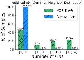
(a) ogbl-collab

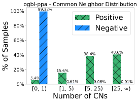
(b) ogbl-ppa

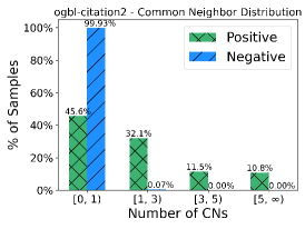
(c) ogbl-citation2

Figure 1: Common neighbor distribution for the positive and negative test samples for the ogbl-collab, ogbl-ppa, and ogbl-citation2 datasets under the existing evaluation setting.

To account for these issues, we propose to first conduct a fair and reproducible evaluation among current link prediction methods under the existing evaluation setting. We then design a new evaluation strategy that is more aligned with a real-world setting and detail our results. Our key contributions are summarized below:

• Reproducible and Fair Comparison. We conduct a fair comparison of different models across multiple common datasets. To ensure a fair comparison, we tune all models on the same set of hyperparameters. We further evaluate different models using multiple types of evaluation metrics. For the Planetoid datasets [17], we further use a unified data split to facilitate a point of comparison between models. To the best of our knowledge, there are no recent efforts to comprehensively benchmark link prediction methods (several exist for KGC [10, 9, 8]). Furthermore, we open-source the implementation in our analysis to enable others in their analyses.

• New Evaluation Setting. We recognize that the current negative sampling strategy used in evaluation is unrealistic and easy. To counter these issues, we first use a more realistic setting of tailoring the negatives to each positive sample. This is achieved by restricting them to be corruptions of the positive sample (i.e., containing one of its two nodes as defined in Eq. (3)). Given the prohibitive cost of utilizing all possible corruptions, we opt instead to only rank against $K$ negatives for each positive sample. In order to choose the most relevant and difficult corruptions, we propose a Heuristic Related Sampling Technique (HeaRT), which selects them based on a combination of multiple heuristics. This creates a more challenging task than the previous evaluation strategy and allows us to better assess the capabilities of current methods.

The rest of the paper is structured as follows. In Section 2 we introduce the models, datasets, and settings used for conducting a fair comparison between methods. In Section 3 we show the results of the fair comparison under the existing evaluation setting and discuss our main observations. Lastly, in Section 4 we introduce our new evaluation setting. We then detail and discuss the performance of different methods using our new setting.

2 Preliminaries

2.1 Task Formulation

In this section we formally define the task of link prediction. Let $\mathcal{G}=\{\mathcal{V},\mathcal{E}\}$ be a graph where $\mathcal{V}$ and $\mathcal{E}$ are the set of nodes and edges in the graph, respectively. Furthermore, let $X\in\mathcal{R}^{\lvert V\rvert\times d}$ be a set of $d$-dimensional features for each node. Link prediction aims to predict the likelihood of a link existing between two nodes given the structural and feature information. For a pair of nodes $u$ and $v$, the probability of a link existing, $p(u,v)$, is therefore given by:

$$p(u,v)=p(u,v\>|\>\mathcal{G},X).$$ (1)

Traditionally, $p(u,v)$ was estimated via non-learnable heuristic methods [24, 25]. More recently, methods that use learnable parameters have gained popularity [12, 13]. These methods attempt to estimate $p(u,v)$ via a learnable function $f$ such that:

$$p(u,v)=f(u,v\>|\>\mathcal{G},X,\Theta),$$ (2)

where $\Theta$ represents a set of learnable parameters. A common choice of $f$ are graph neural networks [26]. In the next subsection we detail the various link prediction methods used in this study.

2.2 Link Prediction Methods

In this section we given an overview of the different methods used in this study. Conventional methods [24, 25] often exploit hand-craft graph structural properties (i.e., heuristics) between node pairs. GNNs attempt to learn the structural information to facilitate link prediction [27, 15, 13]. Given the strong performance of pairwise-based heuristics [14, 15], some recent works use both GNNs and pairwise information, demonstrating strong performance.

For our study, we consider both traditional and state-of-the-art GNN-based models. They can be roughly organized into four categories. 1) Heuristic methods: Common Neighbor (CN) [28], Adamic Adar (AA) [29], Resource Allocation (RA) [30], Shortest Path [25], and Katz [31]. These methods define a score to indicate the link existence based on the graph structure. Among them, CN, AA, and RA are based on the common neighbors, while Shortest Path and Katz are based on the path information. 2) Embedding methods: Matrix factorization (MF) [24], Multilayer Perceptron (MLP) and Node2Vec [32]. These methods are trained to learn low-dimensional node embeddings that are used to predict the likelihood of node pairs existing. 3) GNN methods: GCN [33], GAT [18], SAGE [16], and GAE [20]. These methods attempt to integrate the multi-hop graph structure based on the message passing paradigm. 4) GNN + Pairwise Information methods: Standard GNN methods, while powerful, are not able to capture link-specific information [27]. As such, works have been proposed that augment GNN methods by including additional information to better capture the relation between the nodes in the link we are predicting. SEAL [27], BUDDY [13], and NBFNet [19] use the subgraph features. Neo-GNN [14], NCN [15], and NCNC [15] are based on common neighbor information. Lastly, PEG [34] uses the positional encoding derived from the graph structure.

2.3 Datasets and Experimental Settings

In this section we summarize the datasets and evaluation and training settings. We note that the settings depend on the specific dataset. More details are given in Appendix C.

Datasets. We limit our experiments to homogeneous graphs, which are the most commonly used datasets for link prediction. This includes the small-scale datasets, i.e., Cora, Citeseer, Pubmed [17], and large-scale datasets in the OGB benchmark [23], i.e., ogbl-collab, ogbl-ddi, ogbl-ppa, and ogbl-citation2. We summarize the statistics and split ratio of each dataset in Appendix C.

Metrics. For evaluation, we use both the area under the curve (AUC) and ranking-based metrics, i.e., mean reciprocal rank (MRR) and Hits@K. For Cora, Citeseer, and Pubmed we adopt $K\in\{1,3,10,100\}$. We note that $K=100$ is reported in some recent works [13, 15]). However due to the small number of negatives used during evaluation (e.g., $\approx 500$ for Cora and Citeseer) $K=100$ is likely not informative. For the OGB datasets, we adopt $K\in\{20,50,100\}$ to keep consistent with the original study [23]. Please see Appendix B.1 for the formal definitions of the various evaluation metrics.

Hyperparameter Ranges. We conduct a grid hyperparameter search across a comprehensive range of values. For Cora, Citeseer, and Pubmed this includes: learning rate (0.01, 0.001), dropout (0.1, 0.3, 0.5), weight decay (1e-4, 1e-7, 0), number of model layers (1, 2, 3), number of prediction layers (1, 2, 3), and the embedding size (128, 256). Due to the large size of the OGB datasets, it’s infeasible to tune over such a large range. Therefore, following the most commonly used settings among published hyperparameters, we fix the weight decay to 0, the number of model and prediction layers to be 3, and the embedding size to be 256. The best hyperparameters are chosen based on the validation performance. We note that several exceptions exist to these ranges when they result in significant performance degradations (see Appendix C for more details). We further follow the existing setting and only sample one negative sample per positive sample during training.

Existing Evaluation Settings. In the evaluation stage, the same set of randomly sampled negatives are used for all positive samples. We note that one exception is ogbl-citation2, where they randomly sample 1000 negative samples per positive sample. For Cora, Citeseer, and Pubmed the number of negative samples is equal to the number of positive samples. For the OGB datasets, we use the existing fixed set of randomly chosen negatives found in [23]. Furthermore, for ogbl-collab we follow the existing protocol [23] and include the validation edges in the training graph during testing. This setting is adopted on ogbl-collab under both the existing and new evaluation setting.

Table 1: Results on Cora, Citeseer, and Pubmed(%) under the existing evaluation setting. Highlighted are the results ranked first, second, and third.

Models Cora Citeseer Pubmed MRR AUC MRR AUC MRR AUC Heuristic CN 20.99 70.85 28.34 67.49 14.02 63.9 AA 31.87 70.96 29.37 67.49 16.66 63.9 RA 30.79 70.96 27.61 67.48 15.63 63.9 Shortest Path 12.45 81.08 31.82 75.5 7.15 74.64 Katz 27.4 81.17 38.16 75.37 21.44 74.86 Embedding Node2Vec 37.29 ± 8.82 90.97 ± 0.64 44.33 ± 8.99 94.46 ± 0.59 34.61 ± 2.48 93.14 ± 0.18 MF 14.29 ± 5.79 80.29 ± 2.26 24.80 ± 4.71 75.92 ± 3.25 19.29 ± 6.29 93.06 ± 0.43 MLP 31.21 ± 7.90 95.32 ± 0.37 43.53 ± 7.26 94.45 ± 0.32 16.52 ± 4.14 98.34 ± 0.10 GNN GCN 32.50 ± 6.87 95.01 ± 0.32 50.01 ± 6.04 95.89 ± 0.26 19.94 ± 4.24 98.69 ± 0.06 GAT 31.86 ± 6.08 93.90 ± 0.32 48.69 ± 7.53 96.25 ± 0.20 18.63 ± 7.75 98.20 ± 0.07 SAGE 37.83 ± 7.75 95.63 ± 0.27 47.84 ± 6.39 97.39 ± 0.15 22.74 ± 5.47 98.87 ± 0.04 GAE 29.98 ± 3.21 95.08 ± 0.33 63.33 ± 3.14 97.06 ± 0.22 16.67 ± 0.19 97.47 ± 0.08 GNN+Pairwise Info SEAL 26.69 ± 5.89 90.59 ± 0.75 39.36 ± 4.99 88.52 ± 1.40 38.06 ± 5.18 97.77 ± 0.40 BUDDY 26.40 ± 4.40 95.06 ± 0.36 59.48 ± 8.96 96.72 ± 0.26 23.98 ± 5.11 98.2 ± 0.05 Neo-GNN 22.65 ± 2.60 93.73 ± 0.36 53.97 ± 5.88 94.89 ± 0.60 31.45 ± 3.17 98.71 ± 0.05 NCN 32.93 ± 3.80 96.76 ± 0.18 54.97 ± 6.03 97.04 ± 0.26 35.65 ± 4.60 98.98 ± 0.04 NCNC 29.01 ± 3.83 96.90 ± 0.28 64.03 ± 3.67 97.65 ± 0.30 25.70 ± 4.48 99.14 ± 0.03 NBFNet 37.69 ± 3.97 92.85 ± 0.17 38.17 ± 3.06 91.06 ± 0.15 44.73 ± 2.12 98.34 ± 0.02 PEG 22.76 ± 1.84 94.46 ± 0.34 56.12 ± 6.62 96.15 ± 0.41 21.05 ± 2.85 96.97 ± 0.39

3 Fair Comparison Under the Existing Setting

In this section, we conduct a fair comparison among link prediction methods. This comparison is spurred by the multiple pitfalls noted in Section 1, which include lower-than-actual model performance, multiple data splits, and inconsistent evaluation metrics. These pitfalls hinder our ability to fairly compare different methods. To rectify this, we conduct a fair comparison adhering to the settings listed in section 2.3.

The results are split into two tables. The results for Cora, Citeseer, and Pubmed are shown in Table 1 and OGB in Table 2. For simplicity, we only present the AUC and MRR for Cora, Citeseer, and Pubmed. For OGB datasets, we include AUC and the original ranking metric reported in [23] to allow a convenient comparison ($\text{Hits}@20$ for ogbl-ddi, $\text{Hits}@50$ for ogbl-collab, $\text{Hits}@100$ for ogbl-ppa, and MRR for ogbl-citation2). We use “>24h" to denote methods that require more than 24 hours for either training one epoch or evaluation. OOM indicates that the algorithm requires over 50Gb of GPU memory. Since ogbl-ddi has no node features, we mark the MLP results with a “N/A". Additional results in terms of other metrics are presented in Appendix F. We have several noteworthy observations concerning the methods, the datasets, the evaluation settings, and the overall results. We highlight the main observations below.

Table 2: Results on OGB datasets (%) under the existing evaluation setting. Highlighted are the results ranked first, second, and third.

Models ogbl-collab ogbl-ddi ogbl-ppa ogbl-citation2 Hits@50 AUC Hits@20 AUC Hits@100 AUC MRR Heuristic CN 61.37 82.78 17.73 95.2 27.65 97.22 74.3 AA 64.17 82.78 18.61 95.43 32.45 97.23 75.96 RA 63.81 82.78 6.23 96.51 49.33 97.24 76.04 Shortest Path 46.49 96.51 0 59.07 0 99.13 >24h Katz 64.33 90.54 17.73 95.2 27.65 97.22 74.3 Embedding Node2Vec 49.06 ± 1.04 96.24 ± 0.15 34.69 ± 2.90 99.78 ± 0.04 26.24 ± 0.96 99.77 ± 0.00 45.04 ± 0.10 MF 41.81 ± 1.67 83.75 ± 1.77 23.50 ± 5.35 99.46 ± 0.10 28.4 ± 4.62 99.46 ± 0.10 50.57 ± 12.14 MLP 35.81 ± 1.08 95.91 ± 0.08 N/A N/A 0.45 ± 0.04 90.23 ± 0.00 38.07 ± 0.09 GNN GCN 54.96 ± 3.18 97.89 ± 0.06 49.90 ± 7.23 99.86 ± 0.03 29.57 ± 2.90 99.84 ± 0.03 84.85 ± 0.07 GAT 55.00 ± 3.28 97.11 ± 0.09 31.88 ± 8.83 99.63 ± 0.21 OOM OOM OOM SAGE 59.44 ± 1.37 98.08 ± 0.03 49.84 ± 15.56 99.96 ± 0.00 41.02 ± 1.94 99.82 ± 0.00 83.06 ± 0.09 GAE OOM OOM 7.09 ± 6.02 75.34 ±15.96 OOM OOM OOM GNN+Pairwise Info SEAL 63.37 ± 0.69 95.65 ± 0.29 25.25 ± 3.90 97.97 ± 0.19 48.80 ± 5.61 99.79 ± 0.02 86.93 ± 0.43 BUDDY 64.59 ± 0.46 96.52 ± 0.40 29.60 ± 4.75 99.81 ± 0.02 47.33 ± 1.96 99.56 ± 0.02 87.86 ± 0.18 Neo-GNN 66.13 ± 0.61 98.23 ± 0.05 20.95 ± 6.03 98.06 ± 2.00 48.45 ± 1.01 97.30 ± 0.14 83.54 ± 0.32 NCN 63.86 ± 0.51 97.83 ± 0.04 76.52 ± 10.47 99.97 ± 0.00 62.63 ± 1.15 99.95 ± 0.01 89.27 ± 0.05 NCNC 65.97 ± 1.03 98.20 ± 0.05 70.23 ± 12.11 99.97 ± 0.01 62.61 ± 0.76 99.97 ± 0.01 89.82 ± 0.43 NBFNet OOM OOM >24h >24h OOM OOM OOM PEG 49.02 ± 2.99 94.45 ± 0.89 30.28 ± 4.92 99.45 ± 0.04 OOM OOM OOM

Observation 1: Better than Reported Performance. We find that for some models we are able to achieve superior performance compared to what is reported by recent studies. For instance, in our study Neo-GNN [14] achieves the best overall test performance on ogbl-collab with a Hits@50 of $66.13$. In contrast, the reported performance in [14] is only $57.52$, which would rank seventh under our current setting. This is because the original study [14] does not follow the standard setting of including validation edges in the graph during testing. This setting, as noted in Section 2.3, is used by all other methods on ogbl-collab. However it was omitted by [14], resulting in lower reported performance. Furthermore, on ogbl-citation2 [23], our results for the heuristic methods are typically around $75\%$ MRR. This significantly outperforms previously reported results, which report an MRR of around $50\%$ [27, 13]. The disparity arises as previous studies treat the ogbl-citation2 as a directed graph when applying heuristic methods. However, for GNN-based methods, ogbl-citation2 is typically converted to a undirected graph. We remedy this by also converting ogbl-citation2 to an undirected graph when computing the heuristics, leading to a large increase in performance.

Furthermore, with proper tuning, conventional baselines like GCN [26] and GAE [20] generally exhibit enhanced performance relative to what was originally reported across all datasets. For example, we find that GAE can achieve the second best MRR on Citeseer and GCN the third best Hits@20 on ogbl-ddi. A comparison of the reported results and ours are shown in Table 3. We note that we report AUC for Cora, Citeseer, Pubmed as it was used in the original study. These observations suggest that the performance of various methods are better than what was reported in their initial publications. However, many studies [13, 15, 27] only report the original performance for comparison, which has the potential to lead to inaccurate conclusions.

Table 3: Comparison of ours and the reported results for GCN and GAE.

ogbl-collab ogbl-ppa ogbl-ddi ogbl-citation2 Cora Citeseer Pubmed GCN Hits@50 Hits@100 Hits@20 MRR GAE AUC AUC AUC Reported 47.14 ± 1.45 18.67 ± 1.32 37.07 ± 5.07 84.74 ± 0.21 Reported 91.00 ± 0.01 89.5 ± 0.05 96.4 ± 0.00 Ours 54.96 ± 3.18 29.57 ± 2.90 49.90 ± 7.23 84.85 ± 0.07 Ours 95.08 ± 0.33 97.06 ± 0.22 97.47 ± 0.08

Observation 2: Divergence from Reported Results on ogbl-ddi. We observe that our results in Table 2 for ogbl-ddi differ from the reported results. Outside of GCN, which reports better performance, most other GNN-based methods report a lower-than-reported performance. For example, for BUDDY we only achieve a Hits@20 of 29.60 vs. the reported 78.51 (see Appendix D for a comprehensive comparison among methods). We find that the reason for this difference depends on the method. BUDDY [13] reported using 6 negatives per positive sample during training, leading to an increase in performance. Neo-GNN [14] first pretrains the GNN under the link prediction task, and then uses the pretrained model as the initialization for Neo-GNN. For a fair comparison among methods, we only use 1 negative per positive sample in training and we don’t apply the pretraining. For other methods, we find that a weak relationship between the validation and test performance complicates the tuning process, making it difficult to find the optimal hyperparameters. Please see Appendix E for a more in-depth study and discussion.

Observation 3: High Model Standard Deviation. The results in Tables 1 and 2 present the mean performance and standard deviation when training over 10 seeds. Generally, we find that for multiple datasets the standard deviation of the ranking metrics is often high for most models. For example, the standard deviation for MRR can be as high as $8.82$, $8.96$, or $7.75$ for Cora, Citeseer, and Pubmed, respectively. Furthermore, on ogbl-ddi the standard deviation of Hits@20 reaches as high as 10.47 and 15.56. A high variance indicates unstable model performance. This makes it difficult to compare results between methods as the true performance lies in a larger range. This further complicates replicating model performance, as even large differences with the reported results may still fall within variance (see observation 2). Later in Section 4.3 we find that our new evaluation can reduce the model variance for all datasets (see Table 6). This suggests that the high variance is related to the current evaluation procedure.

Observation 4: Inconsistency of AUC vs. Ranking-Based Metrics. The AUC score is widely adopted to evaluate recent advanced link prediction methods [20, 19]. However, from our results in Tables 1 and 2 we observe that there exists a disparity between AUC and ranking-based metrics. In some cases, the AUC score can be high when the ranking metric is very low or even 0. For example, the Shortest Path heuristic records a Hits@K of 0 on ogbl-ppa. However, the AUC score is $>99\%$. Furthermore, even though RA records the third and fifth best performance on ogbl-ppa and ogbl-collab, respectively, it has a lower AUC score than Shortest Path on both. Previous works [22, 21] argued that AUC is not a proper metric for link prediction. This is due to the inapplicability of AUC for highly imbalanced problems [35, 36].

4 New Evaluation Setting

In this section, we introduce a new setting for evaluating link prediction methods. We first discuss the unrealistic nature of the current evaluation setting in Section 4.1. Based on this, we present our new evaluation setting in Section 4.2, which aims to align better with real-world scenarios. Lastly, in Section 4.3, we present and discuss the results based on our new evaluation setting.

4.1 Issues with the Existing Evaluation Setting

The existing evaluation procedure for link prediction is to rank a positive sample against a set of $K$ randomly selected negative samples. The same set of $K$ negatives are used for all positive samples (with the exception of ogbl-citation2 which uses 1000 per positive sample). We demonstrate that there are multiple issues with this setting, making it difficult to properly evaluate the effectiveness of current models.

Issue 1: Non-Personalized Negative Samples. The existing evaluation setting uses the same set of negative samples for all positive samples (outside of ogbl-citation2). This strategy, referred to as global negative sampling [37], is not a commonly sought objective. Rather, we are often more interested in predicting links that will occur for a specific node. Take, for example, a social network that connects users who are friends. In this scenario, we may be interested in recommending new friends to a user $u$. This requires learning a classifier $f$ that assigns a probability to a link existing. When evaluating this task, we want to rank links where $u$ connects to an existing friend above those where they don’t. For example, if $u$ is friends with $a$ but not $b$, we hope that $f(u,a)>f(u,b)$. However, the existing evaluation setting doesn’t explicitly test for this. Rather it compares a true sample $(u,a)$ with a potentially unrelated negative sample, e.g., $(c,d)$. This is not aligned with the real-world usage of link prediction on such graphs.

Issue 2: Easy Negative Samples. The existing evaluation setting randomly selects negative samples to use. However given the large size of most graphs (see Table 7 in Appendix C), randomly sampled negatives are likely to choose two nodes that bear no relationship to each other. Such node pairs are trivial to classify. We demonstrate this by plotting the distribution of common neighbors (CN), a strong heuristic, for all positive and negative test samples in Figure 1. Almost all the negative samples contain no CNs, making them easy to classify. We further show that the same problem afflicts even the smaller datasets in Figure 3 in Appendix A.

These observations suggest that a more realistic evaluation strategy is desired. At the core of this challenge is which negative samples to use during evaluation. We discuss our design for solving this in the next subsection.

4.2 Heuristic Related Sampling Technique (HeaRT)

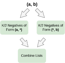
(a) Negative sample generation for one positive sample.

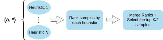
(b) Process of determining negative samples that contain a node $a$.

Figure 2: Pipeline for generating the hard negative samples for a positive sample (a, b).

In this subsection, we introduce new strategy for evaluating link prediction methods. To address the concerns outlined in Section 4.1, we design a new method for sampling negatives during evaluation. Our strategy, HeaRT, solves these challenges by: (a) personalizing the negatives to each sample and (b) using heuristics to select hard negative samples. This allows for the negative samples to be directly related to each positive sample while also being non-trivial. We further discuss how to ensure that the negative samples are both personalized and non-trivial for a specific positive sample.

From our discussion in Section 4.1, we are motivated in personalizing the negatives to each positive sample. Since the positive samples in the current datasets are node pairs, we seek to personalize the negatives to both nodes in the positive sample. Extending our example in Section 4.1, this is analogous to restricting the negatives to contain one of the two users from the original friendship pair. As such, for a positive sample $(u,a)$, the negative samples will belong to the set:

$$S(u,a)=\{(u^{\prime},a)\>|\>u^{\prime}\in\mathcal{V}\}\cup\{(u,a^{\prime})\>|\>a^{\prime}\in\mathcal{V}\},$$ (3)

where $\mathcal{V}$ is the set of nodes. This is similar to the setting used for knowledge graph completion (KGC) [38] which uses all such samples for evaluation. However, one drawback of evaluating each positive sample against the entire set of possible corruptions is the high computational cost. To mitigate this issue we consider only utilizing a small subset of $S(u,a)$ during evaluation.

The key challenge is how to generate a subset of $S(u,a)$. If we randomly sample from $S(u,a)$, we risk only utilizing easy negative samples. This is one of the issues of the existing evaluation setting (see Issue 2 in Section 4.1), whereby randomly selecting negatives, they unknowingly produce negative samples that are too easy. We address this by selecting the negative samples via a combination of multiple heuristics. Since heuristics typically correlate well with performance, we ensure that the negative samples will be non-trivial to classify. This is similar to the concept of candidate generation [39, 40], which only ranks a subset of candidates that are most likely to be true.

An overview of the generation process is given in Figure 2. For each positive sample, we generate $K$ negative samples. To allow personalization to both nodes in the positive sample equally, we sample $K/2$ negatives with each node. For the heuristics, we consider RA [30], PPR [41], and feature similarity. A more detailed discussion on the negative sample generation is given in Appendix G. It’s important to note that our work centers specifically on negative sampling during the evaluation stage (validation and test). This is distinct from prior work that concerns the negatives sampled used during the training phase [42, 43]. As such, the training process remains unaffected under both the existing and HeaRT setting.

Table 4: Results on Cora, Citeseer, and Pubmed (%) under HeaRT. Highlighted are the results ranked first, second, and third.

Models Cora Citeseer Pubmed MRR Hits@10 MRR Hits@10 MRR Hits@10 Heuristic CN 9.78 20.11 8.42 18.68 2.28 4.78 AA 11.91 24.10 10.82 22.20 2.63 5.51 RA 11.81 24.48 10.84 22.86 2.47 4.9 Shortest Path 5.04 15.37 5.83 16.26 0.86 0.38 Katz 11.41 22.77 11.19 24.84 3.01 5.98 Embedding Node2Vec 14.47 ± 0.60 32.77 ± 1.29 21.17 ± 1.01 45.82 ± 2.01 3.94 ± 0.24 8.51 ± 0.77 MF 6.20 ± 1.42 15.26 ± 3.39 7.80 ± 0.79 16.72 ± 1.99 4.46 ± 0.32 9.42 ± 0.87 MLP 13.52 ± 0.65 31.01 ± 1.71 22.62 ± 0.55 48.02 ± 1.79 6.41 ± 0.25 15.04 ± 0.67 GNN GCN 16.61 ± 0.30 36.26 ± 1.14 21.09 ± 0.88 47.23 ± 1.88 7.13 ± 0.27 15.22 ± 0.57 GAT 13.84 ± 0.68 32.89 ± 1.27 19.58 ± 0.84 45.30 ± 1.3 4.95 ± 0.14 9.99 ± 0.64 SAGE 14.74 ± 0.69 34.65 ± 1.47 21.09 ± 1.15 48.75 ± 1.85 9.40 ± 0.70 20.54 ± 1.40 GAE 18.32 ± 0.41 37.95 ± 1.24 25.25 ± 0.82 49.65 ± 1.48 5.27 ± 0.25 10.50 ± 0.46 GNN+Pairwise Info SEAL 10.67 ± 3.46 24.27 ± 6.74 13.16 ± 1.66 27.37 ± 3.20 5.88 ± 0.53 12.47 ± 1.23 BUDDY 13.71 ± 0.59 30.40 ± 1.18 22.84 ± 0.36 48.35 ± 1.18 7.56 ± 0.18 16.78 ± 0.53 Neo-GNN 13.95 ± 0.39 31.27 ± 0.72 17.34 ± 0.84 41.74 ± 1.18 7.74 ± 0.30 17.88 ± 0.71 NCN 14.66 ± 0.95 35.14 ± 1.04 28.65 ± 1.21 53.41 ± 1.46 5.84 ± 0.22 13.22 ± 0.56 NCNC 14.98 ± 1.00 36.70 ± 1.57 24.10 ± 0.65 53.72 ± 0.97 8.58 ± 0.59 18.81 ± 1.16 NBFNet 13.56 ± 0.58 31.12 ± 0.75 14.29 ± 0.80 31.39 ± 1.34 >24h >24h PEG 15.73 ± 0.39 36.03 ± 0.75 21.01 ± 0.77 45.56 ± 1.38 4.4 ± 0.41 8.70 ± 1.26

4.3 Results and Discussion

In this subsection we present our results when utilizing HeaRT. We follow the parameter ranges introduced in Section 2.3. For all datasets we use $K=500$ negative samples per positive sample during evaluation. Furthermore for ogbl-ppa we only use a small subset of the validation and test positive samples (100K each) for evaluation. This is because the large size of the validation and test sets (see Table 7 in Appendix C) makes HeaRT prohibitively expensive.

The results are shown in Table 4 (Cora, Citeseer, Pubmed) and Table  5 (OGB). For simplicity, we only include the MRR and Hits@10 for Cora, Citeseer, Pubmed, and the MRR and Hits@20 for OGB. Additional results for other metrics can be found in Appendix H. We note that most datasets, outside of ogbl-ppa, exhibit much lower performance than under the existing setting. This is though we typically use much fewer negative samples in the new setting, implying that the negative samples produced by HeaRT are much harder. We highlight the main observations below.

Observation 1: Better Performance of Simple Models. We find that under HeaRT, “simple" baseline models (i.e., heuristic, embedding, and GNN methods) show a greater propensity to outperform their counterparts via ranking metrics than under the existing setting. Specifically, we focus on MRR in Table 1, 4, and  5, and the corresponding ranking-based metrics in Table 2. Under the existing setting, such methods only rank in the top three for any dataset a total of 5 times. However, under HeaRT this occurs 10 times. Furthermore, under the existing setting only 1 “simple" method ranks best overall while under HeaRT there are 3. This suggests that recent advanced methods may have benefited from the easier negative samples in the existing setting.

Table 5: Results on OGB datasets (%) under HeaRT. Highlighted are the results ranked first, second, and third.

Models ogbl-collab ogbl-ddi ogbl-ppa ogbl-citation2 MRR Hits@20 MRR Hits@20 MRR Hits@20 MRR Hits@20 CN 4.20 16.46 6.71 38.69 25.70 68.25 17.11 41.73 AA 5.07 19.59 6.97 39.75 26.85 70.22 17.83 43.12 RA 6.29 24.29 8.70 44.01 28.34 71.50 17.79 43.34 Shortest Path 2.66 15.98 0 0 0.54 1.31 >24h >24h Katz 6.31 24.34 6.71 38.69 25.70 68.25 14.10 35.55 Node2Vec 4.68 ± 0.08 16.84 ± 0.17 11.14 ± 0.95 63.63 ± 2.05 18.33 ± 0.10 53.42 ± 0.11 14.67 ± 0.18 42.68 ± 0.20 MF 4.89 ± 0.25 18.86 ± 0.40 13.99 ± 0.47 59.50 ± 1.68 22.47 ± 1.53 70.71 ± 4.82 8.72 ± 2.60 29.64 ± 7.30 MLP 5.37 ± 0.14 16.15 ± 0.27 N/A N/A 0.98 ± 0.00 1.47 ± 0.00 16.32 ± 0.07 43.15 ± 0.10 GCN 6.09 ± 0.38 22.48 ± 0.81 13.46 ± 0.34 64.76 ± 1.45 26.94 ± 0.48 68.38 ± 0.73 19.98 ± 0.35 51.72 ± 0.46 GAT 4.18 ± 0.33 18.30 ± 1.42 12.92 ± 0.39 66.83 ± 2.23 OOM OOM OOM OOM SAGE 5.53 ± 0.5 21.26 ± 1.32 12.60 ± 0.72 67.19 ± 1.18 27.27 ± 0.30 69.49 ± 0.43 22.05 ± 0.12 53.13 ± 0.15 GAE OOM OOM 3.49 ± 1.73 17.81 ± 9.80 OOM OOM OOM OOM SEAL 6.43 ± 0.32 21.57 ± 0.38 9.99 ± 0.90 49.74 ± 2.39 29.71 ± 0.71 76.77 ± 0.94 20.60 ± 1.28 48.62 ± 1.93 BUDDY 5.67 ± 0.36 23.35 ± 0.73 12.43 ± 0.50 58.71 ± 1.63 27.70 ± 0.33 71.50 ± 0.68 19.17 ± 0.20 47.81 ± 0.37 Neo-GNN 5.23 ± 0.9 21.03 ± 3.39 10.86 ± 2.16 51.94 ± 10.33 21.68 ± 1.14 64.81 ± 2.26 16.12 ± 0.25 43.17 ± 0.53 NCN 5.09 ± 0.38 20.84 ± 1.31 12.86 ± 0.78 65.82 ± 2.66 35.06 ± 0.26 81.89 ± 0.31 23.35 ± 0.28 53.76 ± 0.20 NCNC 4.73 ± 0.86 20.49 ± 3.97 >24h >24h 33.52 ± 0.26 82.24 ± 0.40 19.61 ± 0.54 51.69 ± 1.48 NBFNet OOM OOM >24h >24h OOM OOM OOM OOM PEG 4.83 ± 0.21 18.29 ± 1.06 12.05 ± 1.14 50.12 ± 6.55 OOM OOM OOM OOM

Another interesting observation is that on ogbl-collab, heuristic methods achieve strong performance and are able to outperform more complicated models. Specifically, we find that Katz is ranked the second and RA the third. Note that this underscores the significance of the common neighbors information (i.e., paths of length 2), as this information is incorporated in both RA and Katz. Of note is that ogbl-collab is a dynamic collaboration graph, which is different from other datasets. Because of this, the negative sampling strategy also differs slightly from the other datasets. Please see Appendix I for more discussion.

Observation 2: Lower Model Standard Deviation. We observed earlier that, under the existing evaluation setting, the model variance across seeds was high (see observation 3 in Section 3). This complicates model comparison as the model performance is unreliable. Interestingly, we find that HeaRT is able to dramatically reduce the variance for all datasets. We demonstrate this by first calculating the mean standard deviation across all models on each individual dataset. This was done for both evaluation settings with the results compared. As demonstrated in Table 6, the mean standard deviation decreases for all datasets. This is especially true for Cora, Citeseer, and Pubmed, which each decrease by over 85%. Such a large decrease in standard deviation is noteworthy as it allows for a more trustworthy and reliable comparison between methods.

Table 6: Mean model standard deviation for the existing setting and HeaRT. We use Hits@20 for ogbl-ddi, Hits@50 for ogbl-collab, Hits@100 for ogbl-ppa, and MRR otherwise.

Dataset	Existing	HeaRT	% Change
Cora	5.19	0.79	-85%
Citeseer	5.94	0.88	-85%
Pubmed	4.14	0.35	-92%
ogbl-collab	1.49	0.96	-36%
ogbl-ppa	2.13	0.36	-83%
ogbl-ddi	6.77	3.49	-48%
ogbl-citation2	1.39	0.59	-58%

We posit that this observation is caused by a stronger alignment between the positive and negative samples under our new evaluation setting. Under the existing evaluation setting, the same set of negative samples is used for all positive samples. One consequence of this is that a single positive sample may bear little to no relationship to the negative samples (see Section 4.1 for more discussion). However, under our new evaluation setting, the negatives for a positive sample are a subset of the corruptions of that sample. This allows for a more natural comparison via ranking-based metrics as the samples are more related and can be more easily compared.

Observation 3: Lower Model Performance. We observe that the majority of datasets exhibit a significantly reduced performance in comparison to the existing setting. For example, under the existing setting, models typically achieve a MRR of around 30, 50, and 30 on Cora, Citeseer, and Pubmed (Table 1), respectively. However, under HeaRT the MRR for those datasets is typically around 20, 25, and 10 (Table 4). Furthermore for ogbl-citation2, the MRR of the best performing model falls from a shade under 90 on the existing setting to slightly over 20 on HeaRT. Lastly, we note that the performance on ogbl-ppa actually increases. This is because we only utilize a small subset of the total test set when evaluating on HeaRT, nullifying any comparison between the two settings.

These outcomes are observed despite HeaRT using much fewer negative samples than the original setting. This suggests that the negative samples generated by HeaRT are substantially more challenging than those used in the existing setting. This underscores the need to develop more advanced methodologies that can tackle harder negatives samples like in HeaRT.

5 Conclusion

In this work we have revealed several pitfalls found in recent works on link prediction. To overcome these pitfalls, we first establish a benchmarking that facilitates a fair and consistent evaluation across a diverse set of models and datasets. By doing so, we are able to make several illuminating observations about the performance and characteristics of various models. Furthermore, based on several limitations we observed in the existing evaluation procedure, we introduce a more practical setting called HeaRT (Heuristic Related Sampling Technique). HeaRT incorporates a more real-world evaluation setting, resulting in a better comparison among methods. By introducing a more rigorous and realistic assessment, HeaRT could guide the field towards more effective models, thereby advancing the state of the art in link prediction.

6 Acknowledgements

This research is supported by the National Science Foundation (NSF) under grant numbers CNS 2246050, IIS1845081, IIS2212032, IIS2212144, IOS2107215, DUE 2234015, III-2212145, III-2153326, DRL2025244 and IOS2035472, the Army Research Office (ARO) under grant number W911NF-21-1-0198, the Home Depot, Cisco Systems Inc, Amazon Faculty Award, Johnson&Johnson, JP Morgan Faculty Award and SNAP.

7 Checklist

1. For all authors…

   1. Do the main claims made in the abstract and introduction accurately reflect the paper’s contributions and scope? [Yes]

   2. Did you describe the limitations of your work? [Yes] See Appendix K.

   3. Did you discuss any potential negative societal impacts of your work? [Yes] See Appendix L.

   4. Have you read the ethics review guidelines and ensured that your paper conforms to them? [Yes]

2. If you are including theoretical results…

   1. Did you state the full set of assumptions of all theoretical results? [N/A]

   2. Did you include complete proofs of all theoretical results? [N/A]

3. If you ran experiments (e.g. for benchmarks)…

   1. Did you include the code, data, and instructions needed to reproduce the main experimental results (either in the supplemental material or as a URL)? [Yes] See https://github.com/Juanhui28/HeaRT.

   2. Did you specify all the training details (e.g., data splits, hyperparameters, how they were chosen)? [Yes] Yes. See Section 2.3 and Appendix C.

   3. Did you report error bars (e.g., with respect to the random seed after running experiments multiple times)? [Yes]

   4. Did you include the total amount of compute and the type of resources used (e.g., type of GPUs, internal cluster, or cloud provider)? [Yes] See Appendix C.2.

4. If you are using existing assets (e.g., code, data, models) or curating/releasing new assets…

   1. If your work uses existing assets, did you cite the creators? [Yes]

   2. Did you mention the license of the assets? [Yes] See Appendix J.

   3. Did you include any new assets either in the supplemental material or as a URL? [Yes] See https://github.com/Juanhui28/HeaRT.

   4. Did you discuss whether and how consent was obtained from people whose data you’re using/curating? [Yes]

   5. Did you discuss whether the data you are using/curating contains personally identifiable information or offensive content? [N/A]

5. If you used crowdsourcing or conducted research with human subjects…

   1. Did you include the full text of instructions given to participants and screenshots, if applicable? [N/A]

   2. Did you describe any potential participant risks, with links to Institutional Review Board (IRB) approvals, if applicable? [N/A]

   3. Did you include the estimated hourly wage paid to participants and the total amount spent on participant compensation? [N/A]

Appendix A Common Neighbor Distribution

In Figure 1 we demonstrate the common neighbor (CN) distribution among positive and negative test samples for ogbl-collab, ogbl-ppa, and ogbl-citation2. These results demonstrate that a vast majority of negative samples have no CNs. Since CNs is a typically good heuristic, this makes it easy to identify most negative samples.

We further present the CN distribution of Cora, Citeseer, Pubmed, and ogbl-ddi in Figure 3. The CN distribution of Cora, Citeseer, and Pubmed are consistent with our previous observations on the OGB datasets in Figure 1. We note that ogbl-ddi exhibits a different distribution with other datasets. As compared to the other datasets, most of the negative samples in ogbl-ddi have common neighbors. This is likely because ogbl-ddi is considerably denser than the other graphs. As shown in Table 7, the average node degree in ogbl-ddi is $625.68$, significantly larger than the second largest dataset ogbl-ppa with 105.25. Thus, despite the random sampling of negative samples, the high degree of node connectivity within the ogbl-ddi graph predisposes a significant likelihood for the occurrence of common neighbors.

We also present the CN distributions under the HeaRT setting. The plots for Cora, Citeseer, Pubmed are shown in Figure 4. The plots for the OGB datasets are shown in Figure 5. We observe that the CN distribution of HeaRT is more aligned with the positive samples. This allows for a fairer evaluation setting by not favoring models that use CN information.

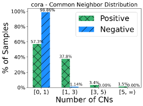
(a) Cora

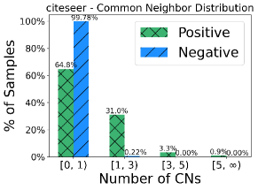
(b) Citeseer

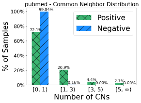
(c) Pubmed

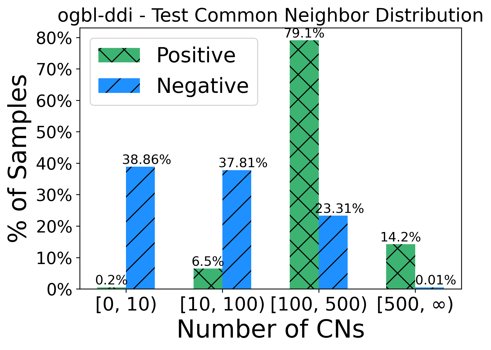
(d) ogbl-ddi

Figure 3: Common neighbor distribution for the positive and negative test samples for the Cora, Citeseer, Pubmed, and ogbl-ddi under the existing evaluation setting.

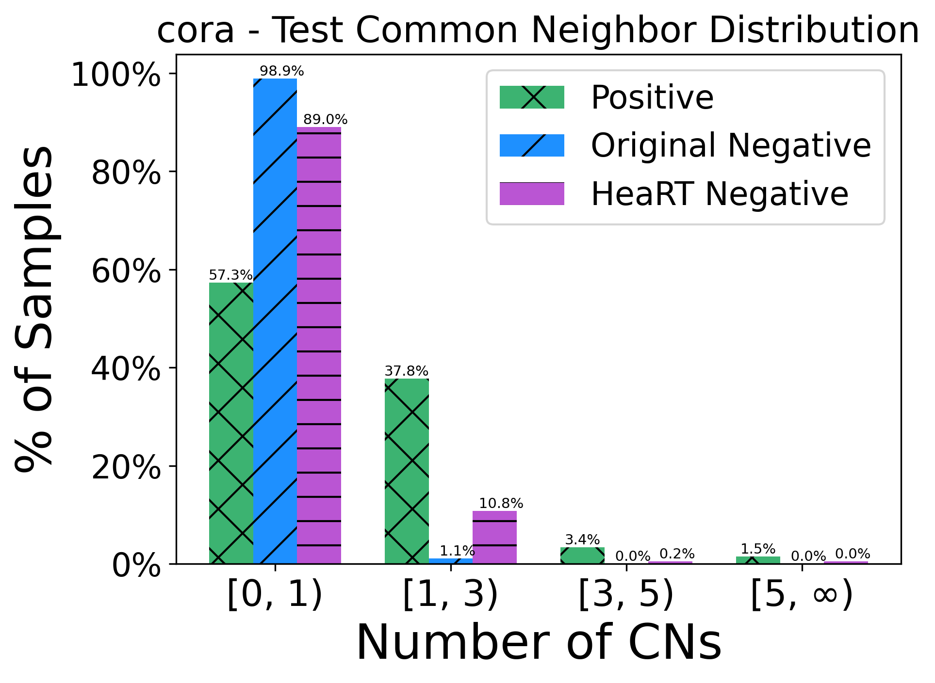
(a) Cora

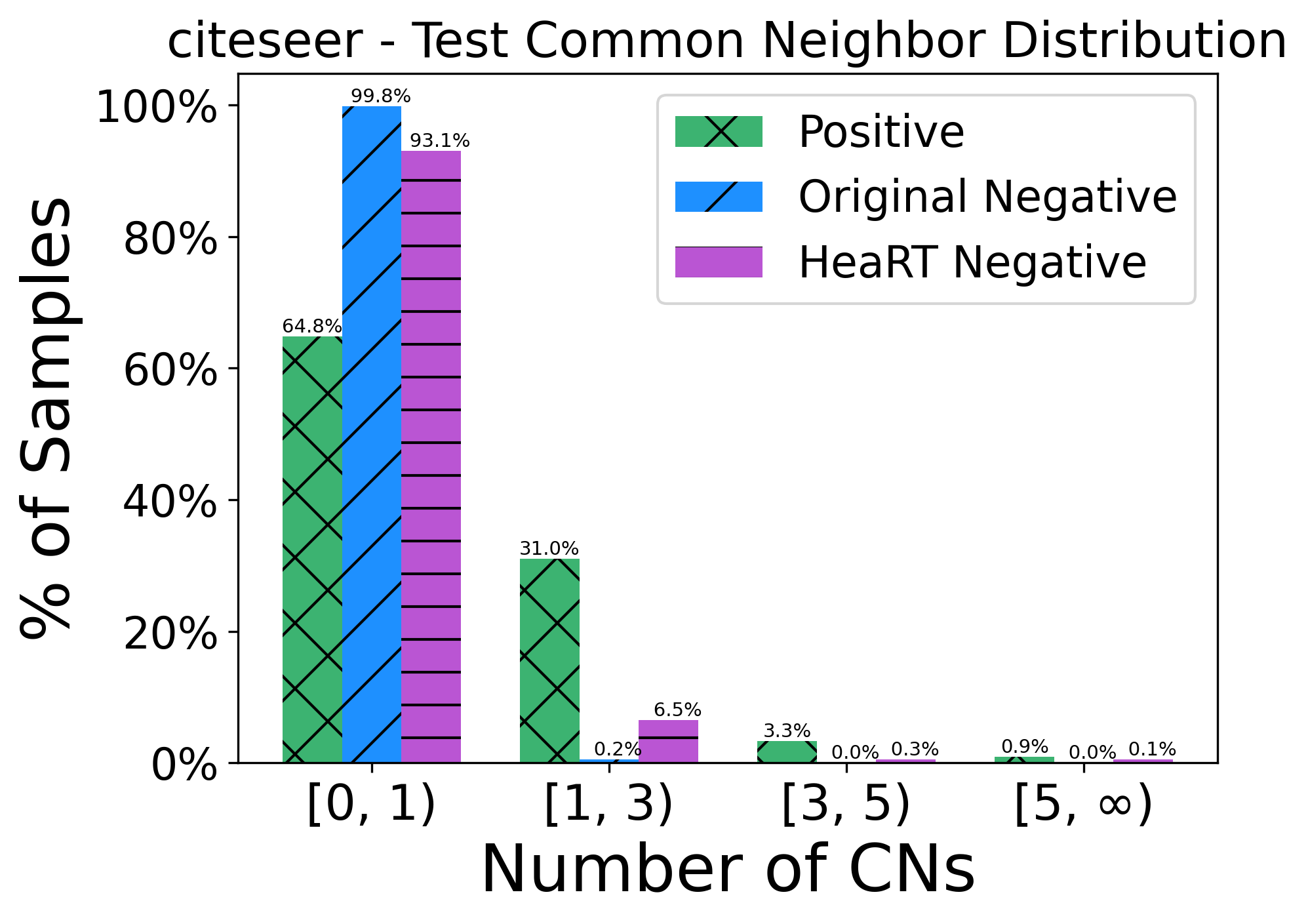
(b) Citeseer

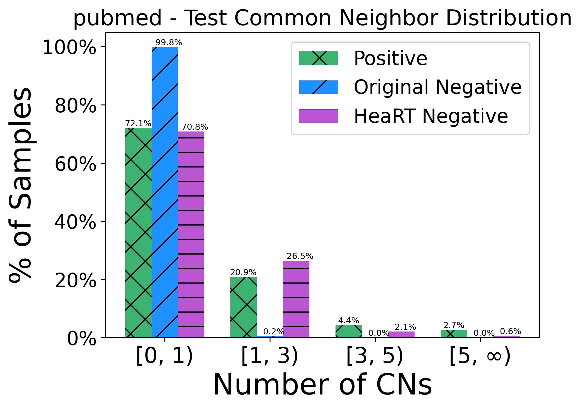
(c) Pubmed

Figure 4: Common neighbor distribution for the positive negative samples under both evaluation settings for Cora, Citeseer, Pubmed.

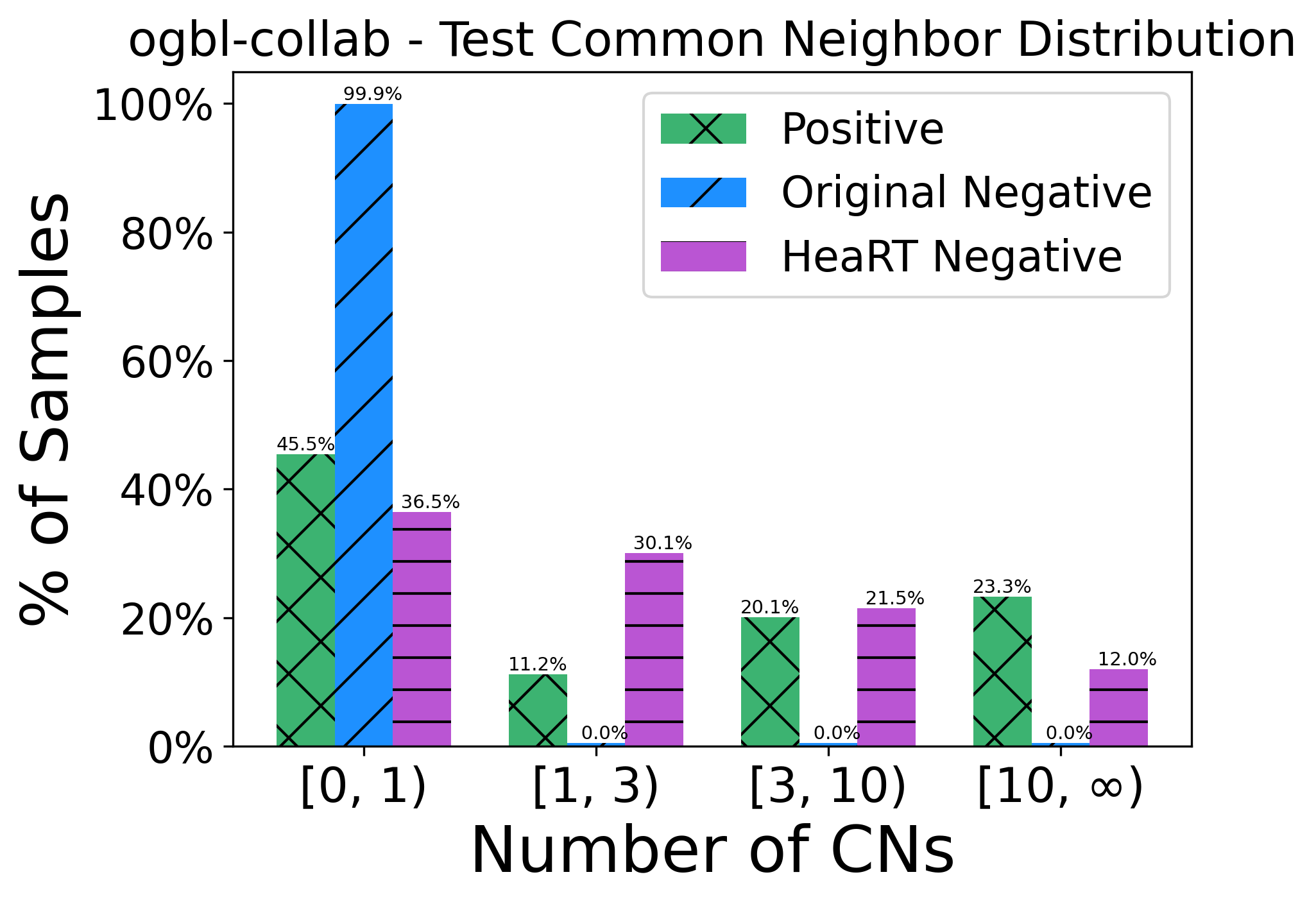
(a) ogbl-collab

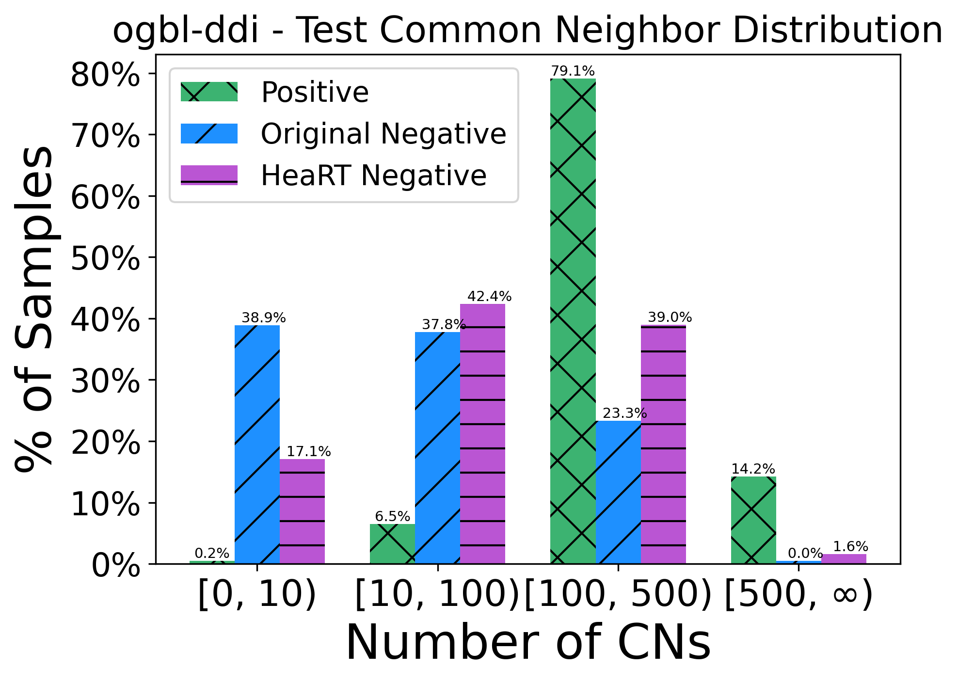
(b) ogbl-ddi

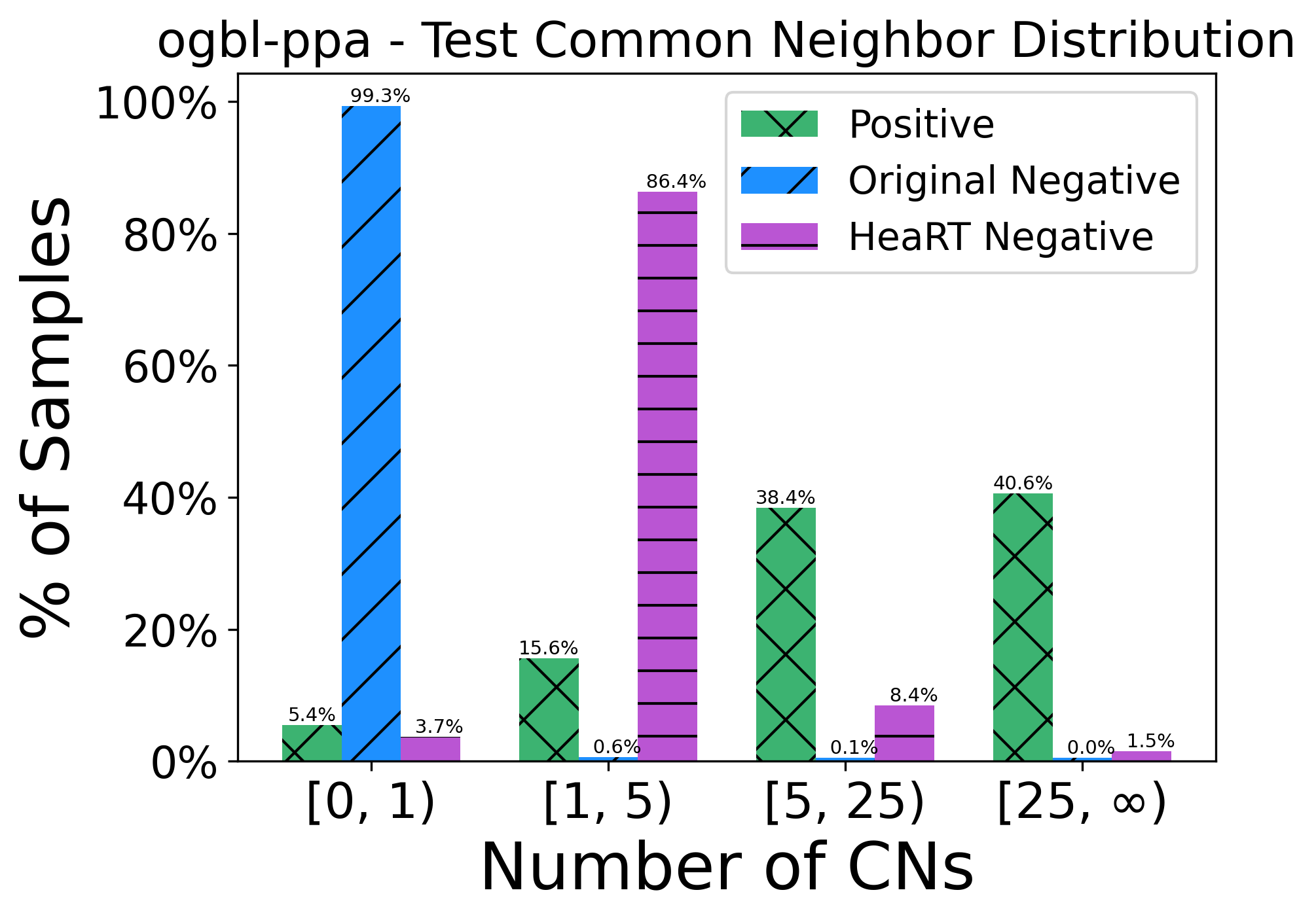
(c) ogbl-ppa

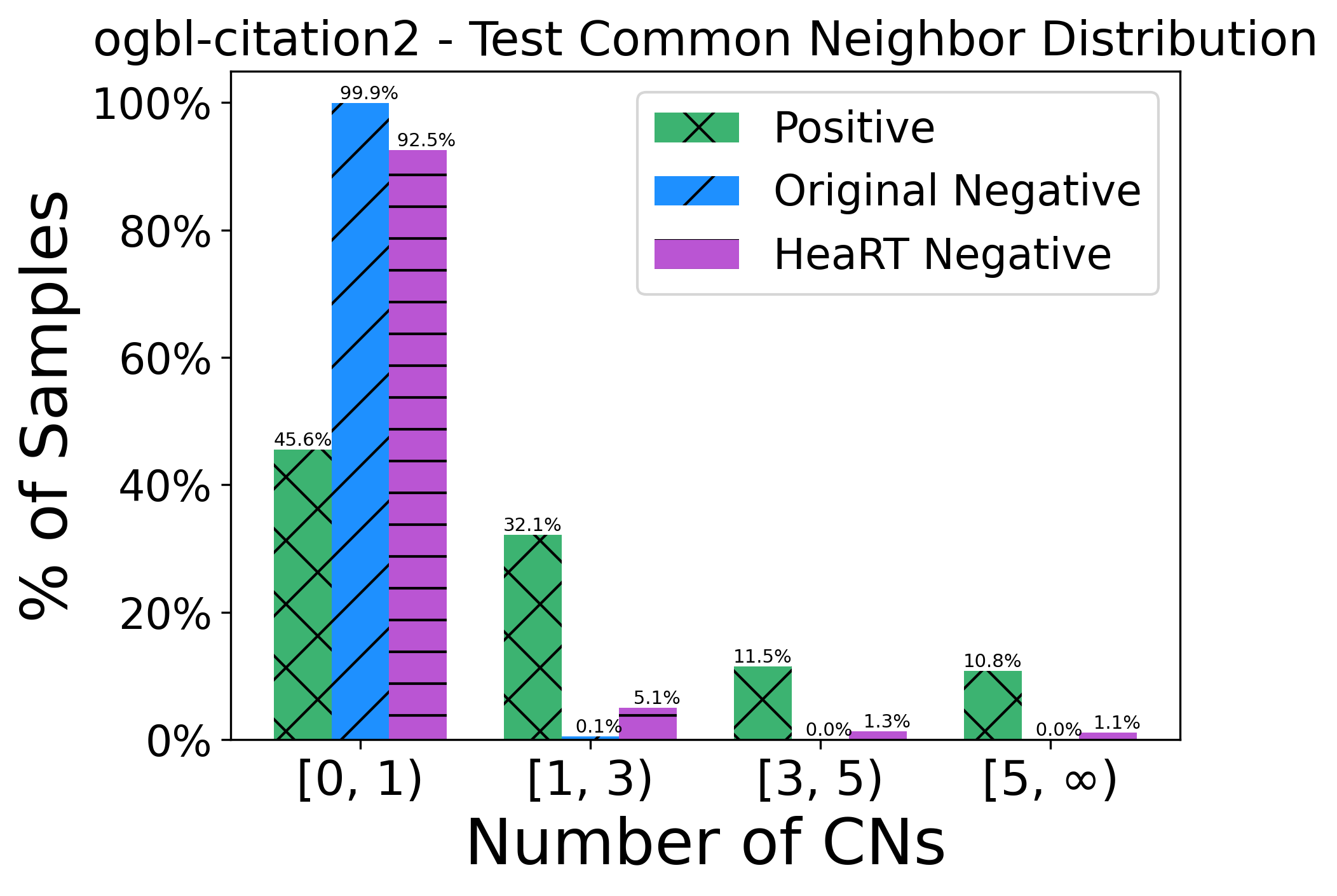
(d) ogbl-citation

Figure 5: Common neighbor distribution for the positive negative samples under both evaluation settings for the OGB datasets.

Appendix B Additional Definitions

B.1 Evaluation Metrics

In this section we define the various evaluation metrics used. Given a single positive sample and $M$ negative samples, we first score each sample and then rank the positive sample among the negatives. The rank is then given by $\text{rank}_{i}$. I.e., a rank of 1 indicates that the positive sample has a higher score than all negatives. The hope is that the positive sample ranks above most or all negative samples. Various metrics make use of this rank. We use $N$ to denote the number of positive samples.

Hits@K. It measures whether the true positive is within the top K predictions or not: $\text{Hits@K}=\frac{1}{N}\sum_{i=1}^{N}\mathbf{1}(\text{rank}_{i}\leq\text{K})$. $\text{rank}_{i}$ is the rank of the $i$-th sample. The indicator function 1 is 1 if $\text{rank}_{i}\leq\text{K}$, and 0 otherwise.

Mean Reciprocal Rank (MRR). It is the mean of the reciprocal rank over all positive samples: $\text{MRR}=\frac{1}{N}\sum_{i=1}^{N}\frac{1}{\text{rank}_{i}}$, where $\text{rank}_{i}$ is the rank of the $i$-th sample.

AUC. It measures the likelihood that a positive sample is ranked higher than a random negative sample: $\text{AUC}=\frac{\sum_{i\in\mathcal{D}^{0}}\sum_{j\in\mathcal{D}^{1}}\mathbf{1}(\text{rank}_{i}<\text{rank}_{j})}{|\mathcal{D}^{0}|\cdot|\mathcal{D}^{1}|}$, where $\mathcal{D}^{0}$ is the set of positive samples, $\mathcal{D}^{1}$ is the set of negative samples, and $\text{rank}_{i}$ is the rank of the $i$-th sample. The indicator function 1 is 1 if $\text{rank}_{i}<\text{rank}_{j}$, and 0 otherwise.

B.2 Negative Sampling

Since only positive links are observed, there is a need to generate negative links (i.e., edges that don’t exist in $\mathcal{G}$) to both train and evaluate different models. We detail how these samples are generated in both training and evaluation.

Training Negative Samples. During training, the negative samples are randomly selected, with all nodes being equally likely to be selected. Let $\mathcal{V}$ and $\mathcal{E}$ be the set of nodes and edges in $\mathcal{G}$. Furthermore, we define $v\in\text{Rand}(\mathcal{V})$ as returning a random node in $\mathcal{V}$. A single negative sample $(a^{-},b^{-})$ is given by:

$$(a^{-},b^{-})=\left(\text{Rand}(\mathcal{V}),\text{Rand}(\mathcal{V})\right).$$ (4)

Typically one negative sample is generated per positive sample.

Evaluation Negative Samples. For the existing setting, a fixed set of randomly selected samples are used as negatives during evaluation. Furthermore, the same set of negative samples are used for each positive sample. This is equivalent to Eq. (4). The only exception is the ogbl-citation2 [23] dataset. For ogbl-citation2, each positive sample is only evaluated against its own set 1000 negative samples. For a positive sample, its negative samples are restricted to contain one of its two nodes (i.e., a corruption). The other node is randomly selected from $\mathcal{V}$. This is equivalent to selecting a set of random samples from the set $S(a,b)$ as defined in Eq. (3).

Appendix C Datasets and Experimental Settings

C.1 Datasets

Table 7: Statistics of datasets. The split ratio is for train/validation/test.

Cora Citeseer Pubmed ogbl-collab ogbl-ddi ogbl-ppa ogbl-citation2 #Nodes 2,708 3,327 18,717 235,868 4,267 576,289 2,927,963 #Edges 5,278 4,676 44,327 1,285,465 1,334,889 30,326,273 30,561,187 Mean Degree 3.9 2.81 4.74 10.90 625.68 105.25 20.88 Split Ratio 85/5/10 85/5/10 85/5/10 92/4/4 80/10/10 70/20/10 98/1/1

The statistics of datasets are shown in Table 7. Generally, Cora, Citeseer, and Pubmed are smaller graphs, with the OGB datasets having more nodes and edges. We adopt the single fixed train/validation/test split with percentages 85/5/10% for Cora, Citeseer, and Pubmed. For OGB datasets, we use the fixed splits provided by the OGB benchmark [23].

C.2 Experimental Settings

Training Settings. We use the binary cross entropy loss to train each model. The loss is optimized using the Adam optimizer [44]. During training we randomly sample one negative sample per positive sample. Each model is trained for a maximum of 9999 epochs, with the process set to terminate when there are no improvements observed in the validation performance over $n$ checkpoints. The choice of $n$ is influenced by both the specific dataset and the complexity of the model. For smaller datasets, such as Cora, Citeseer, and Pubmed, we set $n=50$ uniformly across models (except for NBFNet and SEAL where $n=20$ due to their computational inefficiency). When training on larger OGB datasets, we use a stratified approach: $n=100$ for the simpler methods (i.e., the embedding and GNN-based models) and $n=20$ for the more advanced methods. This is due to the increased complexity and runtime of more advanced methods. An exception is for ogbl-citation2, the largest dataset. To accommodate for its size, we limit the maximum number of epochs to the recommended value from each model’s source code. Furthermore, we set $n=20$ for all models.

In order to accommodate the computational requirements for our extensive experiments, we harness a variety of high-capacity GPU resources. This includes: Tesla V100 32Gb, NVIDIA RTX A6000 48Gb, NVIDIA RTX A5000 24Gb, and Quadro RTX 8000 48Gb.

Table 8: Hyperparameter Search Ranges

Dataset Learning Rate Dropout Weight Decay # Model Layers # Prediction Layers Embedding Dim Cora (0.01, 0.001) (0.1, 0.3, 0.5) (1e-4, 1e-7, 0) (1, 2, 3) (1, 2, 3) (128, 256) Citeseer (0.01, 0.001) (0.1, 0.3, 0.5) (1e-4, 1e-7, 0) (1, 2, 3) (1, 2, 3) (128, 256) Pubmed (0.01, 0.001) (0.1, 0.3, 0.5) (1e-4, 1e-7, 0) (1, 2, 3) (1, 2, 3) (128, 256) ogbl-collab (0.01, 0.001) (0, 0.3, 0.5) 0 3 3 256 ogbl-ddi (0.01, 0.001) (0, 0.3, 0.5) 0 3 3 256 ogbl-ppa (0.01, 0.001) (0, 0.3, 0.5) 0 3 3 256 ogbl-citation2 (0.01, 0.001) (0, 0.3, 0.5) 0 3 3 128

Hyperparameter Settings. We present the hyparameter searching range in Table 8. For the smaller graphs, Cora, Citeseer, and Pubmed, we have a larger search space. However, it’s not feasible to tune over such large space for OGB datasets. By following the most commonly used settings among published hyperparameters, we fix the weight decay, number of model and prediction layers, and the embedding dimension. Furthermore, due to GPU memory constraints, the embedding size is reduced to be 128 for the largest dataset ogbl-citation2.

We note that several exceptions exist to these ranges when they result in significant performance degradations. In such instances, adjustments are guided by the optimal hyperparameters published in the respective source codes. This includes:

• PEG [34]: Adhering to the optimal hyperparameters presented in the source code, when training on ogbl-ddi we set the number of model layers to 2 and the maximum number of epochs to 400.

• NCN/NCNC [15]: When training on ogbl-ddi, we adhere to the suggested optimal hyperparameters used in the source code. Specifically, we set the number of model layers to be 1, and we don’t apply the pretraining for NCNC to facilitate a fair comparison.

• NBFNet [19]: Due to the expensive nature of NBFNet, we further fix the weight decay to 0 when training on Cora, Citeseer, and Pubmed. Furthermore, we follow the suggested hyperparameters  and set the embedding dimension to be 32 and the number of model layers to be 6.

• SEAL [12]: Due to the computational inefficiency of SEAL, when training on Cora, Citeseer and Pubmed we further fix the weight decay to 0. Furthermore, we adhere to the published hyperparameters  and fix the number of model layers to be 3 and the embedding dimension to be 256.

• BUDDY [13]: When training on ogbl-ppa, we incorporate the RA and normalized degree as input features while excluding the raw node features. This is based on the optimal hyperparameters published by the authors.

Appendix D Reported vs. Our Results on ogbl-ddi

In Section 3 (see observation 2), we remarked that there is divergence between the reported results and our results on ogbl-ddi for some methods. A comprehensive comparison of this discrepancy is shown in Table 9. The reported results for Node2Vec, MF, GCN, and SAGE are taken from [23]. The results for the other methods are from their original paper: SEAL [27], BUDDY [13], Neo-GNN [14], NCN [15], NCNC [15], and PEG [34].

Table 9: Comparison results between ours and reported results on ogbl-ddi (Hits@20).

Node2Vec MF GCN SAGE SEAL BUDDY Neo-GNN NCN NCNC PEG Reported 23.26 ± 2.09 13.68 ± 4.75 37.07 ± 5.07 53.90 ± 4.74 30.56 ± 3.86 78.51 ± 1.36 63.57 ± 3.52 82.32 ± 6.10 84.11 ± 3.67 43.80 ± 0.32 Ours 34.69 ± 2.90 23.50 ± 5.35 49.90 ± 7.23 49.84 ± 15.56 25.25 ± 3.90 29.60 ± 4.75 20.95 ± 6.03 76.52 ± 10.47 70.23 ± 12.11 30.28 ± 4.92

Appendix E Additional Investigation on ogbl-ddi

In this section, we present the additional investigation on the ogbl-ddi dataset. In Section E.1 we examine under the existing evaluation setting, there exists a poor relationship between the validation and test performance on ogbl-ddi for many methods. We then demonstrate in Section E.2 that under HeaRT this problem is lessened.

E.1 Existing Evaluation Setting

Upon inspection, we found that there is a poor relationship between the validation and test performance on ogbl-ddi. Since we choose the best hyperparameters based on the validation set, this makes it difficult to properly tune any model on ogbl-ddi. To demonstrate this point, we record the validation and test performance at multiple checkpoints during the training process. The experiments are conducted over 10 seeds. To ensure that our results are not caused by our hyperparameter settings, we use the reported hyperparameters for each model. Lastly, we plot the results for GCN, BUDDY, NCN, and Neo-GNN in Figure 6. It is clear from the results that there exists a poor relationship between the validation and test performance. For example, for NCN, a validation performance of 70 can imply a test performance of 3 to 80. Further investigation is needed to uncover the cause of this misalignment.

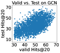
(a) GCN

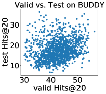
(b) BUDDY

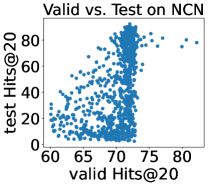
(c) NCN

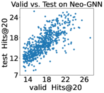
(d) Neo-GNN

Figure 6: Validation vs. test performance for GCN, BUDDY, NCN and Neo-GNN on ogbl-ddi under the existing evaluation setting.

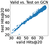
(a) GCN

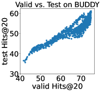
(b) BUDDY

(c) NCN

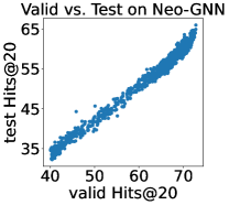
(d) Neo-GNN

Figure 7: Validation vs. test performance when utilizing HeaRT for GCN, BUDDY, NCN and Neo-GNN on ogbl-ddi. We find they have a much stronger relationship than under the existing setting (see Figure 6).

E.2 New Evaluation Setting

Under our new setting, we find that the validation and test performance have a much better relationship. In Section E.1 we observed that there exists a poor relationship between the validation and test performance on ogbl-ddi under the existing evaluation setting. This meddles with our ability to choose the best hyperparameters for each model, as good validation performance is not indicative of good test performance. However, this does not seem to be the case under the new evaluation setting. In Figure 7 we plot the relationship between the validation and test performance by checkpoint for various models. Compared to the same plots under the existing setting (Figure 6), the new results display a much better relationship.

While it’s unclear what is the cause of the poor relationship between the test and validation performance under the existing setting, we conjecture that tailoring the negatives to each positive sample allows for a more natural comparison between a positive sample and its negatives. This may help produce more stable evaluation metrics, thereby strengthening the alignment between the validation and test performance.

Appendix F Additional Results Under the Existing Setting

We present additional results of Cora, Citeseer, Pubmed and OGB datasets in Tables 10-13 under the existing setting. We also omit the MRR for ogbl-collab, ogbl-ddi, and ogbl-ppa. This is because the large number of negative samples make it very inefficient to calculate.

Table 10: Additional results on Cora(%) under the existing evaluation setting. Highlighted are the results ranked first, second, and third.

Models Hits@1 Hits@3 Hits@10 Hits@100 Heuristic CN 13.47 13.47 42.69 42.69 AA 22.2 39.47 42.69 42.69 RA 20.11 39.47 42.69 42.69 Shortest Path 0 0 42.69 71.35 Katz 19.17 28.46 51.61 74.57 Embedding Node2Vec 22.3 ± 11.76 41.63 ± 10.5 62.34 ± 2.35 84.88 ± 0.96 MF 7.76 ± 5.61 13.26 ± 4.52 29.16 ± 6.68 66.39 ± 5.03 MLP 18.79 ± 11.40 35.35 ± 10.71 53.59 ± 3.57 85.52 ± 1.44 GNN GCN 16.13 ± 11.18 32.54 ± 10.83 66.11 ± 4.03 91.29 ± 1.25 GAT 18.02 ± 8.96 42.28 ± 6.37 63.82 ± 2.72 90.70 ± 1.03 SAGE 29.01 ± 6.42 44.51 ± 6.57 63.66 ± 4.98 91.00 ± 1.52 GAE 17.57 ± 4.37 24.82 ± 4.91 70.29 ± 2.75 92.75 ± 0.95 GNN+heuristic SEAL 12.35 ± 8.57 38.63 ± 4.96 55.5 ± 3.28 84.76 ± 1.6 BUDDY 12.62 ± 6.69 29.64 ± 5.71 59.47 ± 5.49 91.42 ± 1.26 Neo-GNN 4.53 ± 1.96 33.36 ± 9.9 64.1 ± 4.31 87.76 ± 1.37 NCN 19.34 ± 9.02 38.39 ± 7.01 74.38 ± 3.15 95.56 ± 0.79 NCNC 9.79 ± 4.56 34.31 ± 8.87 75.07 ± 1.95 95.62 ± 0.84 NBFNet 29.94 ± 5.78 38.29 ± 3.03 62.79 ± 2.53 88.63 ± 0.46 PEG 5.88 ± 1.65 30.53 ± 6.42 62.49 ± 4.05 91.42 ± 0.8

Table 11: Additional results on Citeseer(%) under the existing evaluation setting. Highlighted are the results ranked first, second, and third.

Models Hits@1 Hits@3 Hits@10 Hits@100 Heuristic CN 13.85 35.16 35.16 35.16 AA 21.98 35.16 35.16 35.16 RA 18.46 35.16 35.16 35.16 Shortest Path 0 53.41 56.92 62.64 Katz 24.18 54.95 57.36 62.64 Embedding Node2Vec 30.24 ± 16.37 54.15 ± 6.96 68.79 ± 3.05 89.89 ± 1.48 MF 19.25 ± 6.71 29.03 ± 4.82 38.99 ± 3.26 59.47 ± 2.69 MLP 30.22 ± 10.78 56.42 ± 7.90 69.74 ± 2.19 91.25 ± 1.90 GNN GCN 37.47 ± 11.30 62.77 ± 6.61 74.15 ± 1.70 91.74 ± 1.24 GAT 34.00 ± 11.14 62.72 ± 4.60 74.99 ± 1.78 91.69 ± 2.11 SAGE 27.08 ± 10.27 65.52 ± 4.29 78.06 ± 2.26 96.50 ± 0.53 GAE 54.06 ± 5.8 65.3 ± 2.54 81.72 ± 2.62 95.17 ± 0.5 GNN+heuristic SEAL 31.25 ± 8.11 46.04 ± 5.69 60.02 ± 2.34 85.6 ± 2.71 BUDDY 49.01 ± 15.07 67.01 ± 6.22 80.04 ± 2.27 95.4 ± 0.63 Neo-GNN 41.01 ± 12.47 59.87 ± 6.33 69.25 ± 1.9 89.1 ± 0.97 NCN 35.52 ± 13.96 66.83 ± 4.06 79.12 ± 1.73 96.17 ± 1.06 NCNC 53.21 ± 7.79 69.65 ± 3.19 82.64 ± 1.4 97.54 ± 0.59 NBFNet 17.25 ± 5.47 51.87 ± 2.09 68.97 ± 0.77 86.68 ± 0.42 PEG 39.19 ± 8.31 70.15 ± 4.3 77.06 ± 3.53 94.82 ± 0.81

Table 12: Additional results on Pubmed(%) under the existing evaluation setting. Highlighted are the results ranked first, second, and third.

Models Hits@1 Hits@3 Hits@10 Hits@100 Heuristic CN 7.06 12.95 27.93 27.93 AA 12.95 16 27.93 27.93 RA 11.67 15.21 27.93 27.93 Shortest Path 0 0 27.93 60.36 Katz 12.88 25.38 42.17 61.8 Embedding Node2Vec 29.76 ± 4.05 34.08 ± 2.43 44.29 ± 2.62 63.07 ± 0.34 MF 12.58 ± 6.08 22.51 ± 5.6 32.05 ± 2.44 53.75 ± 2.06 MLP 7.83 ± 6.40 17.23 ± 2.79 34.01 ± 4.94 84.19 ± 1.33 GNN GCN 5.72 ± 4.28 19.82 ± 7.59 56.06 ± 4.83 87.41 ± 0.65 GAT 6.45 ± 10.37 23.02 ± 10.49 46.77 ± 4.03 80.95 ± 0.72 SAGE 11.26 ± 6.86 27.23 ± 7.48 48.18 ± 4.60 90.02 ± 0.70 GAE 1.99 ± 0.12 31.75 ± 1.13 45.48 ± 1.07 84.3 ± 0.31 GNN+heuristic SEAL 30.93 ± 8.35 40.58 ± 6.79 48.45 ± 2.67 76.06 ± 4.12 BUDDY 15.31 ± 6.13 29.79 ± 6.76 46.62 ± 4.58 83.21 ± 0.59 Neo-GNN 19.95 ± 5.86 34.85 ± 4.43 56.25 ± 3.42 86.12 ± 1.18 NCN 26.38 ± 6.54 36.82 ± 6.56 62.15 ± 2.69 90.43 ± 0.64 NCNC 9.14 ± 5.76 33.01 ± 6.28 61.89 ± 3.54 91.93 ± 0.6 NBFNet 40.47 ± 2.91 44.7 ± 2.58 54.51 ± 0.84 79.18 ± 0.71 PEG 8.52 ± 3.73 24.46 ± 6.94 45.11 ± 4.02 76.45 ± 3.83

Table 13: Additional results on OGB datasets(%) under the existing evaluation setting. Highlighted are the results ranked first, second, and third.

ogbl-collab ogbl-ddi ogbl-ppa ogbl-citation2 Hits@20 Hits@100 Hits@50 Hits@100 Hits@20 Hits@50 Hits@20 Hits@50 Hits@100 CN 49.98 65.6 26.51 34.52 13.26 19.67 77.99 77.99 77.99 AA 55.79 65.6 27.07 36.35 14.96 21.83 77.99 77.99 77.99 RA 55.01 65.6 19.14 31.17 25.64 38.81 77.99 77.99 77.99 Shortest Path 46.49 66.82 0 0 0 0 >24h >24h >24h Katz 58.11 71.04 26.51 34.52 13.26 19.67 78 78 78 Node2Vec 40.68 ± 1.75 55.58 ± 0.77 59.19 ± 3.61 73.49 ± 3.18 11.22 ± 1.91 19.22 ± 1.69 82.8 ± 0.13 92.33 ± 0.1 96.44 ± 0.03 MF 39.99 ± 1.25 43.22 ± 1.94 45.51 ± 11.13 61.72 ± 6.56 9.33 ± 2.83 21.08 ± 3.92 70.8 ± 12.0 74.48 ± 10.42 75.5 ± 10.13 MLP 27.66 ± 1.61 42.13 ± 1.09 N/A N/A 0.16 ± 0.0 0.26 ± 0.03 74.16 ± 0.1 86.59 ± 0.08 93.14 ± 0.06 GCN 44.92 ± 3.72 62.67 ± 2.14 74.54 ± 4.74 85.03 ± 3.41 11.17 ± 2.93 21.04 ± 3.11 98.01 ± 0.04 99.03 ± 0.02 99.48 ± 0.02 GAT 43.59 ± 4.17 62.24 ± 2.29 55.46 ± 10.16 69.74 ± 10.01 OOM OOM OOM OOM OOM SAGE 50.77 ± 2.33 65.36 ± 1.05 93.48 ± 1.36 97.37 ± 0.55 19.37 ± 2.65 31.3 ± 2.36 97.48 ± 0.03 98.75 ± 0.03 99.3 ± 0.02 GAE OOM OOM 12.39 ± 8.74 14.03 ± 9.22 OOM OOM OOM OOM OOM SEAL 54.19 ± 1.57 69.94 ± 0.72 43.34 ± 3.23 52.2 ± 1.78 21.81 ± 4.3 36.88 ± 4.06 94.61 ± 0.11 95.0 ± 0.12 95.37 ± 0.14 BUDDY 57.78 ± 0.59 67.87 ± 0.87 53.36 ± 2.57 71.04 ± 2.56 26.33 ± 2.63 38.18 ± 1.32 97.79 ± 0.07 98.86 ± 0.04 99.38 ± 0.03 Neo-GNN 57.05 ± 1.56 71.76 ± 0.55 33.88 ± 10.1 46.55 ± 13.29 26.16 ± 1.24 37.95 ± 1.45 97.05 ± 0.07 98.75 ± 0.03 99.41 ± 0.02 NCN 50.27 ± 2.72 67.58 ± 0.09 95.51 ± 0.87 97.54 ± 0.7 40.29 ± 2.22 53.35 ± 1.77 97.97 ± 0.03 99.02 ± 0.02 99.5 ± 0.01 NCNC 54.91 ± 2.84 70.91 ± 0.25 92.34 ± 2.42 96.35 ± 0.52 40.1 ± 1.06 52.09 ± 1.99 97.22 ± 0.78 98.2 ± 0.71 98.77 ± 0.6 NBFNet OOM OOM >24h >24h OOM OOM OOM OOM OOM PEG 33.57 ± 7.40 55.14 ± 2.10 47.93 ± 3.18 59.95 ± 2.52 OOM OOM OOM OOM OOM

Appendix G Additional Details on HeaRT

As described in Section 4.2, given a positive sample $(a,b)$, we seeks to generate $K$ negative samples to evaluate against. The negative samples are drawn from the set of possible corruptions of $(a,b)$, i.e, $S(a,b)$ (see Eq. (3)). Multiple heuristics are used to determine which $K$ negative samples to use. Furthermore, the negative samples are split evenly between both nodes. That is, we generate $K/2$ negative samples that contain either node $a$ and $b$, respectively. This process is illustrated in Figure 2.

The rest of this section is structured as follows. In Section G.1 we describe how we use multiple heuristics for estimating the difficulty of negative samples. Then in Section G.2 we describe how we combine the ranks given by different heuristic methods.

G.1 Determining Hard Negative Samples

We are first tasked with how to choose the negative samples. As discussed and shown in Section 4.2, we want to select the negative samples from $S(a,b)$ such that they are non-trivial to classify. Hence, as inspired by the candidate generation process in real-world recommender systems [39, 40], we aim to select a set of ’hard’ negative samples that are more relevant to the source node. The candidate generation process is typically based on some primitive and simple link prediction heuristics. These heuristics can be also treated as link prediction methods (see Tables 1 and 2).

We use multiple heuristics that capture a variety of different information. Most link prediction heuristics can be categorized into two main categories: local heuristics and global heuristics [1]. Local heuristics attempt to capture the local neighborhood information that exists near the node pair while global heuristics attempt to use the whole graph structure. To capture the local information we use resource allocation (RA) [30], a CN-based approach. Existing results show that RA can achieve strong performance on most datasets (see Tables 1 and 2). To measure the global information we use the personalized pagerank score (PPR) [41]. Random walk based methods are commonly used for candidate generation [39, 40]. Lastly, we further include the cosine feature similarity for the Cora, Citeseer, and Pubmed datasets. This is due to the strong performance of a MLP on those datasets. By combining these heuristics, we are able to generate a diverse set of negative samples for each positive sample.

For each heuristic we then rank all the possible negative samples. We first denote the score of a heuristic $i$ for a pair of nodes $a$ and $b$ as $h_{i}(a,b)$. Let’s say we want to rank all negative samples that contain a node $a$, i.e., $(a,*)$. The rank across all nodes is given by:

$$R_{i}=\underset{v\in\bar{V}}{\text{ArgSort}}\;h_{i}(a,v),$$ (5)

where $R_{i}$ denotes the ranking for heuristic $i$ and and $\bar{V}$ is a subset of the set of nodes in the graph $V$. We apply a filtering process to exclude all positive training samples, self-loops, and the sample itself under consideration from being selected as negative samples. Additionally, when choosing negative samples for the test samples, we disallow validation samples to be chosen as well. As such, we only consider a subset of nodes $\bar{V}\in V$. This is analogous to the filtered setting used in KGC [38]. However, we adopt a distinct filtering strategy for the ogbl-collab dataset, which is a dynamic collaboration graph. Specifically, positive training samples are not excluded in the generation of negative samples for validation and test. Similarly, positive validation samples are not omitted when creating negative test samples. This approach is justified for ogbl-collab which is a dynamic graph, as prior collaboration between authors does not necessarily indicates future collaborations. Further details and discussions are provided in Appendix I.

We now have all possible negative samples ranked according to multiple heuristics. However, it is unclear how to choose the negative samples from multiple ranked lists. In the next subsection we detail how we combine the ranks according to each heuristic. This will give us a final ranking, of which we can choose the top $K/2$ as the negative samples for that node.

G.2 Combining Heuristic Ranks

In this subsection we tackle the problem of combing the negative sample ranks given by multiple heuristics. More concretely, say we use $m$ heuristics and rank all the samples according to each. We want to arrive at a combined ranking $R_{\text{total}}$ that is composed of each rank,

$$R_{\text{total}}=\phi(R_{1},R_{2},\cdots,R_{m}).$$ (6)

We model $\phi$ via Borda’s method [45]. Let $R_{i}(a,v)$ be the rank of the node pair $(a,v)$ for heuristic $i$. The combined rank $R_{\text{total}}(a,v)$ across $m$ ranked lists is given by:

$$R_{\text{total}}(a,v)=g\left(R_{1}(a,v),R_{2}(a,v),\cdots,R_{m}(a,v)\right),$$ (7)

where $g$ is an aggregation function. We set $g=\text{min}(\cdot)$. This is done as it allows us to capture a more distinct set of samples by selecting the “best" for each heuristic. This is especially true when there is strong disagreement between the different heuristics. A final ranking is then done on $R_{\text{total}}$ to select the top nodes,

$$R_{f}=\underset{v\in\bar{V}}{\text{ArgSort}}\;R_{\text{total}},$$ (8)

where $R_{f}$ is the final ranking. The highest $K/2$ nodes are then selected from $R_{f}$. Lastly, we note that for some nodes there doesn’t exist sufficient scores to rank $K/2$ total nodes. In this case the remaining nodes are chosen randomly. The full generation process for a node $a$ is detailed in Algorithm 1.

Algorithm 1 Generating Negative Samples of Form $(a,*)$

1:

2:$a=$ Node to generate samples for

3:$\bar{V}=$ Possible nodes to use for negative samples

4:$\mathcal{H}=\{h_{1},h_{2},\cdots,h_{m}\}$ $\triangleright$ Set of $m$ heuristics

5:for $i\in\lvert\mathcal{H}\rvert$ do

6:     $R_{i}=\underset{v\in\bar{V}}{\text{ArgSort}}\;h_{i}(a,v)$ $\triangleright$ Sort by each heuristic individually

7:end for

8:for $v\in\bar{V}$ do

9:     $R_{\text{total}}(a,v)=\text{min}\left(R_{1}(a,v),R_{2}(a,v),\cdots,R_{m}(a,v)\right)$ $\triangleright$ Combine the rankings

10:end for

11:$R_{f}=\underset{v\in\bar{V}}{\text{ArgSort}}\;R_{\text{total}}(a,v)$ $\triangleright$ Sort by combined ranking

12:return $R_{f}[:K/2]$ $\triangleright$ Return the top K/2 ranked nodes

Appendix H Additional Results Under HeaRT

We present additional results of Cora, Citeseer, Pubmed, and OGB datasets under HeaRT in Table 14 and Table 15. These results include other hit metrics not found in the main tables.

Table 14: Additional results on Cora, Citeseer, and Pubmed(%) under HeaRT. Highlighted are the results ranked first, second, and third.

Cora Citeseer Pubmed Models Hits1 Hits3 Hits100 Hits1 Hits3 Hits100 Hits1 Hits3 Hits100 CN 3.98 10.25 38.71 2.2 9.45 33.63 0.47 1.49 19.29 AA 5.31 12.71 38.9 3.96 12.09 33.85 0.74 1.87 20.37 RA 5.31 12.52 38.52 4.18 11.21 34.07 0.72 1.78 20.04 Shortest Path 0.57 2.85 55.6 0.22 3.52 53.85 0 0.02 21.57 Katz 4.64 11.95 59.96 3.74 11.87 55.82 0.74 2.12 32.78 Node2Vec 5.69 ± 0.81 15.1 ± 0.99 77.21 ± 2.34 9.63 ± 0.82 23.5 ± 1.37 84.46 ± 1.86 0.75 ± 0.14 2.4 ± 0.32 52.27 ± 0.65 MF 1.46 ± 0.8 5.46 ± 1.67 59.68 ± 3.41 2.68 ± 0.92 7.25 ± 0.98 53.25 ± 2.91 1.13 ± 0.24 3.25 ± 0.44 50.56 ± 1.11 MLP 5.48 ± 0.99 14.15 ± 1.56 77.0 ± 1.02 10.44 ± 0.82 26.46 ± 1.24 86.83 ± 1.36 1.28 ± 0.22 4.33 ± 0.28 76.34 ± 0.79 GCN 7.59 ± 0.61 17.46 ± 0.82 85.47 ± 0.52 9.27 ± 0.99 23.19 ± 0.98 89.1 ± 2.13 2.09 ± 0.31 5.58 ± 0.27 73.59 ± 0.53 GAT 5.03 ± 0.81 13.66 ± 0.67 80.87 ± 1.32 8.02 ± 1.21 20.09 ± 0.82 86.83 ± 1.09 1.14 ± 0.16 3.06 ± 0.36 67.06 ± 0.69 SAGE 5.48 ± 0.97 15.43 ± 1.07 81.61 ± 0.96 8.37 ± 1.62 23.74 ± 1.62 92.33 ± 0.68 3.03 ± 0.46 8.19 ± 1.0 79.47 ± 0.53 GAE 9.72 ± 0.73 19.24 ± 0.76 79.66 ± 0.95 13.81 ± 0.82 27.71 ± 1.34 85.49 ± 1.37 1.48 ± 0.23 4.05 ± 0.39 59.79 ± 0.67 SEAL 3.89 ± 2.04 10.82 ± 4.04 61.9 ± 13.97 5.08 ± 1.31 13.68 ± 1.32 68.94 ± 2.3 1.47 ± 0.32 4.71 ± 0.68 65.81 ± 2.43 BUDDY 5.88 ± 0.60 13.76 ± 1.03 82.46 ± 1.79 10.09 ± 0.50 26.11 ± 1.26 92.66 ± 0.92 2.24 ± 0.17 5.93 ± 0.21 72.01 ± 0.46 Neo-GNN 5.71 ± 0.41 13.89 ± 0.82 80.28 ± 1.08 6.81 ± 0.73 17.8 ± 1.19 85.51 ± 1.01 1.90 ± 0.24 6.07 ± 0.47 76.57 ± 0.58 NCN 4.85 ± 0.81 14.46 ± 0.98 84.14 ± 1.24 16.77 ± 2.05 30.51 ± 0.97 90.42 ± 0.98 1.13 ± 0.18 3.95 ± 0.24 71.46 ± 0.97 NCNC 4.78 ± 0.71 14.72 ± 1.24 85.62 ± 0.83 11.14 ± 0.82 27.21 ± 0.96 92.73 ± 1.16 2.73 ± 0.49 7.05 ± 0.72 79.22 ± 0.96 NBFNet 5.31 ± 1.16 14.95 ± 0.72 76.24 ± 0.68 5.95 ± 1.06 14.53 ± 1.19 72.66 ± 0.95 >24h >24h >24h PEG 6.98 ± 0.57 14.93 ± 0.61 82.52 ± 1.28 9.93 ± 0.6 21.91 ± 0.59 90.15 ± 1.43 0.88 ± 0.18 2.61 ± 0.39 64.95 ± 1.81

Table 15: Additional results on OGB datasets(%) under HeaRT. Highlighted are the results ranked first, second, and third.

ogbl-collab ogbl-ddi ogbl-ppa ogbl-citation2 Models Hits50 Hits100 Hits50 Hits100 Hits50 Hits100 Hits50 Hits100 CN 30.52 42.80 70.12 86.53 80.53 86.51 57.56 68.04 AA 33.74 45.20 71.08 87.36 81.93 87.55 58.87 69.39 RA 36.68 46.42 76.39 90.96 81.65 86.84 58.88 68.83 Shortest Path 33.77 45.85 0 0 1.34 1.4 >24h >24h Katz 39.18 48.80 70.12 86.53 80.53 86.51 54.97 67.56 Node2Vec 28.56 ± 0.17 41.84 ± 0.25 98.38 ± 0.7 99.91 ± 0.01 69.94 ± 0.06 81.88 ± 0.06 61.22 ± 0.16 77.11 ± 0.13 MF 30.83 ± 0.22 43.23 ± 0.34 95.52 ± 0.72 99.54 ± 0.08 83.29 ± 3.35 89.75 ± 1.9 29.64 ± 7.3 65.87 ± 8.37 MLP 28.88 ± 0.32 46.83 ± 0.33 N/A N/A 5.36 ± 0.0 22.01 ± 0.01 61.29 ± 0.07 76.94 ± 0.1 GCN 35.29 ± 0.49 50.83 ± 0.21 97.65 ± 0.68 99.85 ± 0.06 81.48 ± 0.48 89.62 ± 0.23 70.77 ± 0.34 85.43 ± 0.18 GAT 32.92 ± 1.41 46.71 ± 0.84 98.15 ± 0.24 99.93 ± 0.02 OOM OOM OOM OOM SAGE 33.48 ± 1.40 48.33 ± 0.49 99.17 ± 0.11 99.98 ± 0.01 81.84 ± 0.24 89.46 ± 0.13 71.91 ± 0.1 85.86 ± 0.09 GAE OOM OOM 28.29 ± 13.65 48.34 ± 15.0 OOM OOM OOM OOM SEAL 33.57 ± 0.84 43.06 ± 1.09 82.42 ± 3.37 92.63 ± 2.05 87.34 ± 0.49 92.45 ± 0.26 65.11 ± 2.33 77.64 ± 2.43 BUDDY 39.04 ± 0.11 50.49 ± 0.09 97.81 ± 0.31 99.93 ± 0.01 82.5 ± 0.51 88.36 ± 0.32 67.47 ± 0.32 81.94 ± 0.26 Neo-GNN 36.11 ± 2.36 49.25 ± 0.81 83.45 ± 11.03 94.7 ± 4.82 81.21 ± 1.39 88.31 ± 0.19 62.14 ± 0.51 79.13 ± 0.42 NCN 34.53 ± 0.98 45.69 ± 0.42 98.43 ± 0.22 99.96 ± 0.01 89.37 ± 0.28 93.11 ± 0.27 71.56 ± 0.03 84.01 ± 0.05 NCNC 34.96 ± 3.80 46.93 ± 2.04 >24h >24h 91.0 ± 0.24 94.72 ± 0.18 72.85 ± 0.9 86.35 ± 0.51 NBFNet OOM OOM >24h >24h OOM OOM OOM OOM PEG 30.12 ± 0.63 45.40 ± 0.66 84.21 ± 9.2 95.76 ± 3.48 OOM OOM OOM OOM

Appendix I Additional Investigation on ogbl-collab

Table 16: Results on ogbl-collab under HeaRT when excluding the positive train/validation samples of being negative samples during testing. Highlighted are the results ranked first, second, and third.

MRR Hits20 Hits50 Hits100 CN 12.60 27.51 38.39 47.4 AA 16.40 32.65 42.61 50.25 RA 28.14 41.16 46.9 51.78 Shortest Path 46.71 46.56 46.97 48.11 Katz 47.15 48.66 51.07 54.28 Node2Vec 12.10 ± 0.20 25.85 ± 0.21 35.49 ± 0.22 46.12 ± 0.34 MF 26.86 ± 1.74 38.44 ± 0.07 43.62 ± 0.08 51.75 ± 0.14 MLP 12.61 ± 0.66 23.05 ± 0.89 35.32 ± 0.74 51.09 ± 0.37 GCN 18.28 ± 0.84 32.90 ± 0.66 43.17 ± 0.36 54.93 ± 0.14 GAT 10.97 ± 1.16 29.58 ± 2.42 42.07 ± 1.51 53.45 ± 0.64 SAGE 20.89 ± 1.06 33.83 ± 0.93 43.02 ± 0.63 54.38 ± 0.27 GAE OOM OOM OOM OOM SEAL 22.53 ± 3.51 36.48 ± 2.55 43.5 ± 1.75 49.25 ± 1.39 BUDDY 32.42 ± 1.88 45.62 ± 0.52 50.57 ± 0.18 55.63 ± 0.68 Neo-GNN 21.90 ± 0.65 38.40 ± 0.29 46.93 ± 0.17 53.81 ± 0.19 NCN 17.51 ± 2.50 37.07 ± 2.97 45.89 ± 1.11 52.36 ± 0.33 NCNC 19.02 ± 5.32 35.67 ± 6.78 44.76 ± 4.64 52.41 ± 2.09 NBFNet OOM OOM OOM OOM PEG 15.68 ± 1.10 29.74 ± 0.95 38.71 ± 0.17 49.34 ± 0.70

As introduced in Section G.1, we adopt a different strategy to generate the hard negative samples for ogbl-collab which is a dynamic collaboration graph. In this dataset, nodes represent authors and edges represent a collaboration between two authors. Each edge further includes an attribute that specifies the year of collaboration. Specifically, each edge takes the form of (Author 1, Year, Author 2). The task is to predict collaborations in 2019 (test) based on those until 2017 (training) and 2018 (validation).

Contrary to other datasets, we do not exclude the positive training samples when generating the negative samples for validation and test. We note that we also do not exclude positive validation edges when generating the negatives for test. In simpler terms, when creating negative samples for testing, both positive samples from training and validation are considered. This means that negative samples during testing could present in the training and validation positive samples. This approach is reasonable and well-aligned with the real-world scenario in the context of collaboration graphs. Specifically, authors who collaborated in the past might not do so in the future. For instance, just because the positive sample (Author 2, 2017, Author 3) exists, it does not imply that (Author 2, 2019, Author 3) is also true. However, this is implied to be true if we exclude positive train/validation samples from appearing as negative samples during testing.

We validate this approach by contrasting it with the strategy that excludes train/validation data when generating hard negatives. The results are presented in Table 16. We observed that under this setting, both the Shortest Path and Katz perform considerably well on ogbl-collab. Specifically, the MRR gap between the second-ranked method (Shortest Path) and the third (BUDDY) is 14.29. We found that it is due to the ogbl-collab being a dynamic graph. Of the positive samples in the test set, around $46\%$ also appear as positive samples in the training set. In particular, an edge (Author 1, 2017, Author 2) in the training data may also “appear” in the test data in the form of (Author 1, 2019, Author 2). This is because two authors who collaborated in the past often tend to collaborate again in the future. As such, when evaluating the test sample (Author 1, 2019, Author 2), there exists path of length 1 between the two authors in the graph. Furthermore, this phenomenon is common among positive samples but not observed among negatives. This is because we exclude the positive training samples when generating the negative samples for evaluation. As a result of this exclusion, the presence of a direct link (i.e., a shortest path of length 1) between two authors suggest a positive sample, while its absence often corresponds to a negative sample. As such, it provides an easy “shortcut” to distinguish positive and negative samples during testing. This explains why methods like Shortest Path and Katz can achieve good performance on ogbl-collab when excluding positive train/validation samples of being negative samples during testing.

On the contrary, when allowing positive train/validation samples to also be negative samples for HeaRT, the results on ogbl-collab, shown in Tables 5 and 15, indicate that Shortest Path does not maintain its superior performance as observed in Table 16. Additionally, the overall results under HeaRT are inferior to the ones in Table 5. For instance, while all the MRR values in Table 5 exceed 10, the highest MRR in Table 16 is approximately 6. This indicates that excluding those positive samples from being negative samples disproportionately helps the Shortest Path.

Appendix J Dataset Licenses

The license for each dataset can be found in Table 17.

Table 17: Dataset Licenses.

Datasets License Cora NLM License Citeseer NLM License Pubmed NLM License ogbl-collab MIT License ogbl-ddi MIT License ogbl-ppa MIT License ogbl-citation2 MIT License

Appendix K Limitation

One potential limitation of HeaRT lies in the generation of customized negative samples for each positive sample. This design may result in an increased number of negative samples compared to the existing setting. Although this provides a more realistic evaluation, it could have an impact on the efficiency of the evaluation process, especially in scenarios where a significant number of positive samples exist. Nonetheless, this limitation does not detract from the potential benefits of HeaRT in providing a more realistic and meaningful link prediction evaluation setting. Furthermore, as each evaluation node pair is independent, it offers scope for parallelization, mitigating any potential efficiency concerns to a large extent. Future work can investigate ways to optimize this process.

Appendix L Social Impact

Our method HeaRT harbors significant potential for positive societal impact. By aligning the evaluation setting more closely with real-world scenarios, it enhances the applicability of link prediction research. This not only contributes to the refinement of existing prediction methods but also stimulates the development of more effective link prediction methods. As link prediction has far-reaching implications across numerous domains, from social network analysis to recommendation systems and beyond, improving its performance and accuracy is of paramount societal importance. We also carefully consider the broader impact from various perspectives such as fairness, security, and harm to people. No apparent risk is related to our work.

References

- [1] Linyuan Lü and Tao Zhou. Link prediction in complex networks: A survey. Physica A: statistical mechanics and its applications, 390(6):1150–1170, 2011.
- [2] Nur Nasuha Daud, Siti Hafizah Ab Hamid, Muntadher Saadoon, Firdaus Sahran, and Nor Badrul Anuar. Applications of link prediction in social networks: A review. Journal of Network and Computer Applications, 166:102716, 2020.
- [3] István A Kovács, Katja Luck, Kerstin Spirohn, Yang Wang, Carl Pollis, Sadie Schlabach, Wenting Bian, Dae-Kyum Kim, Nishka Kishore, Tong Hao, et al. Network-based prediction of protein interactions. Nature communications, 10(1):1240, 2019.
- [4] Zan Huang, Xin Li, and Hsinchun Chen. Link prediction approach to collaborative filtering. In Proceedings of the 5th ACM/IEEE-CS joint conference on Digital libraries, pages 141–142, 2005.
- [5] Zonghan Wu, Shirui Pan, Fengwen Chen, Guodong Long, Chengqi Zhang, and S Yu Philip. A comprehensive survey on graph neural networks. IEEE transactions on neural networks and learning systems, 32(1):4–24, 2020.
- [6] Oleksandr Shchur, Maximilian Mumme, Aleksandar Bojchevski, and Stephan Günnemann. Pitfalls of graph neural network evaluation. arXiv preprint arXiv:1811.05868, 2018.
- [7] Federico Errica, Marco Podda, Davide Bacciu, and Alessio Micheli. A fair comparison of graph neural networks for graph classification. In Proceedings of the 8th International Conference on Learning Representations (ICLR), 2020.
- [8] Daniel Ruffinelli, Samuel Broscheit, and Rainer Gemulla. You can teach an old dog new tricks! on training knowledge graph embeddings. In International Conference on Learning Representations.
- [9] Mehdi Ali, Max Berrendorf, Charles Tapley Hoyt, Laurent Vermue, Mikhail Galkin, Sahand Sharifzadeh, Asja Fischer, Volker Tresp, and Jens Lehmann. Bringing light into the dark: A large-scale evaluation of knowledge graph embedding models under a unified framework. IEEE Transactions on Pattern Analysis and Machine Intelligence, 44(12):8825–8845, 2021.
- [10] Zhiqing Sun, Shikhar Vashishth, Soumya Sanyal, Partha Talukdar, and Yiming Yang. A re-evaluation of knowledge graph completion methods. In Proceedings of the 58th Annual Meeting of the Association for Computational Linguistics, pages 5516–5522, 2020.
- [11] Vijay Prakash Dwivedi, Chaitanya K Joshi, Anh Tuan Luu, Thomas Laurent, Yoshua Bengio, and Xavier Bresson. Benchmarking graph neural networks. Journal of Machine Learning Research, 24(43):1–48, 2023.
- [12] Muhan Zhang and Yixin Chen. Link prediction based on graph neural networks. Advances in neural information processing systems, 31, 2018.
- [13] Benjamin Paul Chamberlain, Sergey Shirobokov, Emanuele Rossi, Fabrizio Frasca, Thomas Markovich, Nils Hammerla, Michael M Bronstein, and Max Hansmire. Graph neural networks for link prediction with subgraph sketching. arXiv preprint arXiv:2209.15486, 2022.
- [14] Seongjun Yun, Seoyoon Kim, Junhyun Lee, Jaewoo Kang, and Hyunwoo J Kim. Neo-gnns: Neighborhood overlap-aware graph neural networks for link prediction. Advances in Neural Information Processing Systems, 34:13683–13694, 2021.
- [15] Xiyuan Wang, Haotong Yang, and Muhan Zhang. Neural common neighbor with completion for link prediction. arXiv preprint arXiv:2302.00890, 2023.
- [16] Will Hamilton, Zhitao Ying, and Jure Leskovec. Inductive representation learning on large graphs. Advances in neural information processing systems, 30, 2017.
- [17] Zhilin Yang, William Cohen, and Ruslan Salakhudinov. Revisiting semi-supervised learning with graph embeddings. In International conference on machine learning, pages 40–48. PMLR, 2016.
- [18] Petar Velickovic, Guillem Cucurull, Arantxa Casanova, Adriana Romero, Pietro Lio, and Yoshua Bengio. Graph attention networks. stat, 1050:20, 2017.
- [19] Zhaocheng Zhu, Zuobai Zhang, Louis-Pascal Xhonneux, and Jian Tang. Neural bellman-ford networks: A general graph neural network framework for link prediction. Advances in Neural Information Processing Systems, 34:29476–29490, 2021.
- [20] Thomas N Kipf and Max Welling. Variational graph auto-encoders. arXiv preprint arXiv:1611.07308, 2016.
- [21] Yang Yang, Ryan N Lichtenwalter, and Nitesh V Chawla. Evaluating link prediction methods. Knowledge and Information Systems, 45(3):751–782, 2015.
- [22] Zexi Huang, Mert Kosan, Arlei Silva, and Ambuj Singh. Link prediction without graph neural networks. arXiv preprint arXiv:2305.13656, 2023.
- [23] Weihua Hu, Matthias Fey, Marinka Zitnik, Yuxiao Dong, Hongyu Ren, Bowen Liu, Michele Catasta, and Jure Leskovec. Open graph benchmark: Datasets for machine learning on graphs. Advances in neural information processing systems, 33:22118–22133, 2020.
- [24] Aditya Krishna Menon and Charles Elkan. Link prediction via matrix factorization. In Joint european conference on machine learning and knowledge discovery in databases, pages 437–452. Springer, 2011.
- [25] David Liben-Nowell and Jon Kleinberg. The link prediction problem for social networks. In Proceedings of the twelfth international conference on Information and knowledge management, pages 556–559, 2003.
- [26] Thomas N. Kipf and Max Welling. Semi-supervised classification with graph convolutional networks. In International Conference on Learning Representations (ICLR), 2017.
- [27] Muhan Zhang, Pan Li, Yinglong Xia, Kai Wang, and Long Jin. Labeling trick: A theory of using graph neural networks for multi-node representation learning. Advances in Neural Information Processing Systems, 34:9061–9073, 2021.
- [28] Mark EJ Newman. Clustering and preferential attachment in growing networks. Physical review E, 64(2):025102, 2001.
- [29] Lada A Adamic and Eytan Adar. Friends and neighbors on the web. Social networks, 25(3):211–230, 2003.
- [30] Tao Zhou, Linyuan Lü, and Yi-Cheng Zhang. Predicting missing links via local information. The European Physical Journal B, 71:623–630, 2009.
- [31] Leo Katz. A new status index derived from sociometric analysis. Psychometrika, 18(1):39–43, 1953.
- [32] Aditya Grover and Jure Leskovec. node2vec: Scalable feature learning for networks. In Proceedings of the 22nd ACM SIGKDD international conference on Knowledge discovery and data mining, pages 855–864, 2016.
- [33] Liang Yao, Chengsheng Mao, and Yuan Luo. Graph convolutional networks for text classification. In Proceedings of the AAAI conference on artificial intelligence, volume 33, pages 7370–7377, 2019.
- [34] Haorui Wang, Haoteng Yin, Muhan Zhang, and Pan Li. Equivariant and stable positional encoding for more powerful graph neural networks. arXiv preprint arXiv:2203.00199, 2022.
- [35] Jesse Davis and Mark Goadrich. The relationship between precision-recall and roc curves. In Proceedings of the 23rd international conference on Machine learning, pages 233–240, 2006.
- [36] Takaya Saito and Marc Rehmsmeier. The precision-recall plot is more informative than the roc plot when evaluating binary classifiers on imbalanced datasets. PloS one, 10(3):e0118432, 2015.
- [37] Zhitao Wang, Yong Zhou, Litao Hong, Yuanhang Zou, Hanjing Su, and Shouzhi Chen. Pairwise learning for neural link prediction. arXiv preprint arXiv:2112.02936, 2021.
- [38] Antoine Bordes, Nicolas Usunier, Alberto Garcia-Duran, Jason Weston, and Oksana Yakhnenko. Translating embeddings for modeling multi-relational data. Advances in neural information processing systems, 26, 2013.
- [39] Pankaj Gupta, Ashish Goel, Jimmy Lin, Aneesh Sharma, Dong Wang, and Reza Zadeh. Wtf: The who to follow service at twitter. In Proceedings of the 22nd international conference on World Wide Web, pages 505–514, 2013.
- [40] Chantat Eksombatchai, Pranav Jindal, Jerry Zitao Liu, Yuchen Liu, Rahul Sharma, Charles Sugnet, Mark Ulrich, and Jure Leskovec. Pixie: A system for recommending 3+ billion items to 200+ million users in real-time. In Proceedings of the 2018 world wide web conference, pages 1775–1784, 2018.
- [41] Sergey Brin and Lawrence Page. The anatomy of a large-scale hypertextual web search engine. Computer networks and ISDN systems, 30(1-7):107–117, 1998.
- [42] Zhen Yang, Ming Ding, Chang Zhou, Hongxia Yang, Jingren Zhou, and Jie Tang. Understanding negative sampling in graph representation learning. In Proceedings of the 26th ACM SIGKDD international conference on knowledge discovery & data mining, pages 1666–1676, 2020.
- [43] Steffen Rendle, Christoph Freudenthaler, Zeno Gantner, and Lars Schmidt-Thieme. Bpr: Bayesian personalized ranking from implicit feedback. In Proceedings of the Twenty-Fifth Conference on Uncertainty in Artificial Intelligence, pages 452–461, 2009.
- [44] Diederik P Kingma and Jimmy Ba. Adam: A method for stochastic optimization. arXiv preprint arXiv:1412.6980, 2014.
- [45] JC de Borda. M’emoire sur les’ elections au scrutin. Histoire de l’Acad’emie Royale des Sciences, 1781.