In-Process Global Interpretation for Graph Learning via Distribution Matching

Abstract

Graphs neural networks (GNNs) have emerged as a powerful graph learning model due to their superior capacity in capturing critical graph patterns. To gain insights about the model mechanism for interpretable graph learning, previous efforts focus on post-hoc local interpretation by extracting the data pattern that a pre-trained GNN model uses to make an individual prediction. However, recent works show that post-hoc methods are highly sensitive to model initialization and local interpretation can only explain the model prediction specific to a particular instance. In this work, we address these limitations by answering an important question that is not yet studied: how to provide global interpretation of the model training procedure? We formulate this problem as in-process global interpretation, which targets on distilling high-level and human-intelligible patterns that dominate the training procedure of GNNs. We further propose Graph Distribution Matching (GDM) to synthesize interpretive graphs by matching the distribution of the original and interpretive graphs in the feature space of the GNN as its training proceeds. These few interpretive graphs demonstrate the most informative patterns the model captures during training. Extensive experiments on graph classification datasets demonstrate multiple advantages of the proposed method, including high explanation accuracy, time efficiency and the ability to reveal class-relevant structure.

1 Introduction

Graph neural networks (GNNs) [29, 7, 14, 30, 15, 25] have attracted enormous attention for graph learning, but they are usually treated as black boxes, which may raise trustworthiness concerns if humans cannot really interpret what pattern exactly a GNN model learns and justify its decisions. Lack of such understanding could be particularly risky when using a GNN model for high-stakes domains (e.g., finance [32] and medicine [5]), which highlights the importance of ensuring a comprehensive interpretation of the working mechanism for GNNs.

To improve transparency and understand the behavior of GNNs, most recent works focus on providing post-hoc interpretation, which aims at explaining what patterns a pre-trained GNN model uses to make decisions [31, 18, 34, 28]. However, recent studies have shown that such a pre-train-then-explain manner would fail to provide faithful explanations: their interpretations may suffer from the bias attribution issue [6], the overfitting and initialization issue (i.e., explanation accuracy is sensitive to the pre-trained model) [21]. In contrast, in-process interpretation probes to the while training procedure of GNN models to interpret the patterns learned during training, which is not aggressively depended on a single pre-trained model thus results in more stable interpretations. However, in-process interpretation has been rarely investigated for graph learning.

Existing works generate in-process interpretation by constructing inherently interpretable models, which either suffer from a trade-off between the prediction accuracy and interpretability [4, 33] or can only provide local interpretations on individual instances [21]. Specifically, local interpretations [21, 31, 18] focus on explaining the model decision for a particular graph instance, which requires manual inspections on many local interpretations to mitigate the variance across instances and conclude a high-level pattern of the model behavior. The majority of existing interpretation techniques belong to this category. As a sharp comparison to such instance-specific interpretations, global interpretations [34, 28] aim at understanding the general behavior of the model with respect to different classes, without relying on any particular instance.

To address the limitations of post-hoc and local interpretation methods, for the first time, we attempt to provide in-process global interpretation for the graph learning procedure, which targets on distilling high-level and human-intelligible patterns the model learns to differentiate different classes. Specifically, we propose Graph Distribution Matching (GDM) to synthesize a few compact interpretive graphs for each class following the distribution matching principle: the interpretive graphs should follow similar distribution as the original graphs in the dynamic feature space of the GNN model as its training progresses. We optimize interpretive graphs by minimizing the distance between the interpretive and original data distributions, measured by the maximum mean discrepancy (MMD) [9] in a family of embedding spaces obtained by the GNN model. Presumably, GDM simulates the model training behavior, thus the generated interpretation can provide a general understanding of patterns that dominate the model training.

Different from post-hoc interpretation, our in-process interpretation concludes patterns from the whole training trajectory, thus is less biased to a single pre-trained model and is more stable; and compared with local interpretation, our global interpretation does not rely on individual graph instance, thus is a more general reflection of the model behavior. Our perspective provides a complementary view to the extensively studied post-hoc local interpretability, and our work puts an important step towards a more comprehensive understanding of graph learning.

Extensive quantitative evaluations on six synthetic and real-world graph classification datasets verify the interpretation effectiveness of GDM. The experimental results show that GDM can be used as a probe to precisely generate small interpretive graphs that preserve sufficient information for model training in an efficient manner, and the captured patterns are class discriminative. A qualitative study is also conducted to intuitively demonstrate human-intelligible interpretive graphs.

2 Related Work

Due to the prevalence of graph neural networks (GNNs), extensive efforts have been conducted to improve their transparency and interpretability. Existing interpretation techniques can be categorized as post-hoc and in-process interpretation depending on the interpretation stage, or local and global interpretation depending on the interpretation form.

Post-hoc versus In-process Interpretations Most existing GNN interpretation methods we have found are post-hoc methods [31, 19, 34, 28]. Post-hoc interpretability methods target on a pre-trained model and learn the underlying important features or nodes by querying the model’s output. However, recent studies [21, 6] found that their explanations are sensitive to the pre-trained model: not all pre-trained models will lead to the best interpretation. And they suffer from the overfitting issue: interpretation performance starts to decrease after several epochs. Our in-process interpretation generates explanation graphs by inspecting the whole training trajectory of GNNs, not only the last snapshot, and thus is more stable and less prone to overfitting.

We only found one in-process interpretation method for graph learning, Graph Stochastic Attention (GSAT) [21], which is based on the information bottleneck principle and incorporates stochasticity into attention weights. While GSAT regards attention scores as interpretations, and are generated during the training procedure, it can only provide local interpretation, i.e., the attention is on each individual graph instance, thus cannot conclude general interpretation patterns without inspecting many instances. As a contrast, GDM provides a global interpretation for each class following the distribution matching principle.

Local versus Global Interpretations Local interpretation methods such as GNNExplainer [31] and PGExplainer [19] provide input-dependent explanations for each input graph. Given an input graph, these methods explain GNNs by outputting a small, explainable graph with important features. According to [36], there are four types of instance-level explanation frameworks for GNN. They are gradient-based [22], perturbation-based [31, 18], decomposition-based [11], and surrogate-based methods [27]. While local interpretations help explain predictions on individual graph instances, local interpretation cannot answer what common features are shared by graph instances for each class. Therefore, it is necessary to have both instance-level local and model-level global interpretations.

XGNN [34] and GNNInterpreter [28] are the only works that we found providing a global explanation of GNNs. In detail, XGNN leverages a reinforcement learning framework where for each step, the graph generator predicts how to add an edge to the current graph. Finally, it explains GNNs by training a graph generator so that the generated graph patterns maximize a certain prediction of the model. Specifically, XGNN leverages domain-experts knowledge for making rewards function for different inputs. GNNInterpreter learns a probabilistic generative graph distribution and identifies graph pattern when GNN tries to make a certain prediction by optimizing a objective function consisting of the likelihood of the explanation graph being predicted as a target class by the GNN model and a similarity regularization term. However, these two works are essentially post-hoc methods for a pre-trained GNN, and inherit the aforementioned issues of post-hoc interpretation. Our GDM instead is the first work studying the in-process global interpretation problem for graph learning.

3 Methods

We first discuss existing post-hoc methods and provide a general form covering both local and global interpretation. To understand model training behavior, we for the first time formulate a new form of in-process interpretation. Based on this general form, we propose to generate interpretations by synthesizing a few compact graphs via distribution matching, which can be formulated as an optimization problem. We further discuss several practical constraints for optimizing interpretive graphs. Finally, we provide an overview and algorithm for the proposed interpretation method.

3.1 Notations and Background for Graph Learning

We first introduce the notations for formulating the interpretation problem. We focus on explaining GNNs’ training behavior for the graph classification task. A graph classification dataset with $N$ graphs can be denoted as $\mathcal{G}=\{G^{(1)},G^{(2)},\dots,G^{(N)}\}$ with a corresponding ground-truth label set $\mathcal{Y}=\{y^{(1)},y^{(2)},\dots,y^{(N)}\}$. Each graph consists of two components, $G^{(i)}=(\textbf{A}^{(i)},\textbf{X}^{(i)})$, where $\textbf{A}^{(i)}\in\{0,1\}^{n\times n}$ denotes the adjacency matrix and $\textbf{X}^{(i)}\in\mathbb{R}^{n\times d}$ is the node feature matrix. The label for each graph is chosen from a set of $C$ classes $y^{(i)}\in\{1,\dots,C\}$, and we use $y^{(i)}_{c}$ to denote the label of graph $G_{i}$ is $c$, that is $y^{(i)}=c$. We further denote a set of graphs that belong to class $c$ as $\mathcal{G}_{c}=\{G^{(i)}|y^{(i)}=c\}$. A GNN model $\Phi(\cdot)$ is a concatenation of a feature extractor $f_{\bm{\theta}}(\cdot)$ parameterized by $\bm{\theta}$ and a classifier $h_{\bm{\psi}}(\cdot)$ parameterized by $\bm{\psi}$, that is $\Phi(\cdot)=h_{\bm{\psi}}(f_{\bm{\theta}}(\cdot))$. The feature extractor $f_{\bm{\theta}}:\mathcal{G}\rightarrow\mathbb{R}^{d^{\prime}}$ takes in a graph and embeds it to a low dimensional space with $d^{\prime}\ll d$. The classifier $h_{\bm{\psi}}:\mathbb{R}^{d^{\prime}}\rightarrow\{1,\dots,C\}$ further outputs the predicted class given the graph embedding.

3.2 Revisit Post-hoc Interpretation Problem

We first provide a general form for existing post-hoc interpretations. The goal of post-hoc interpretation is to explain the inference behavior of a pre-trained GNN model, e.g., what patterns lead a GNN model to make a certain decision. Specifically, given a pre-trained GNN model $\Phi^{*}$, post-hoc interpretation method finds the patterns that maximize the predicted probability for a class $y_{c}$. Formally, this problem can be defined as:

$$\min_{\mathcal{S}}\mathcal{L}(\Phi^{*}(\mathcal{S}),y_{c}),$$ (1)

where $\mathcal{S}$ is one or a set of small graphs absorbing important graph structures and node features for interpretation, and $\mathcal{L}(\cdot,\cdot)$ is the loss (e.g., cross-entropy loss) of predicting $\mathcal{S}$ as label $y_{c}$. Existing post-hoc interpretation techniques can fit in this form but differ in the definition of $\mathcal{S}$. We take two representative works, GNNExplainer [31] and XGNN [34], as an example of post-hoc local and post-hoc global interpretation, respectively.

GNNExplainer [31] is a post-hoc local interpretation method. In this work, $\mathcal{S}$ is a compact subgraph extracted from an input instance $G_{o}=(\textbf{A}_{o},\textbf{X}_{o})$, defined as $\mathcal{S}_{\text{GNNExplainer}}=(\textbf{A}_{o}\odot\sigma(M),\textbf{X}_{o})$, where $\sigma(M)$ is a soft mask, $M$ denotes a mask matrix to be optimized for masking unimportant edges in the adjacency matrix, $\sigma$ denotes a sigmoid function, and $\odot$ denoted element-wise multiplication. The label of the input instance $G_{o}$ determines $y_{c}$.

XGNN [34] is a post-hoc global interpretation method. It defines $\mathcal{S}$ as a set of completely synthesized graphs with each edge generated by reinforcement learning. The goal of the reward function is to maximize the probability of predicting $\mathcal{S}$ as a certain class $y_{c}$.

Discussion As shown in Eq.(1), the post-hoc interpretation is a post-analysis of a pre-trained GNN model $\Phi^{*}$. As discussed in [21], these post-hoc methods often fail to provide stable interpretation: the interpreter could be easily over-fitted to the pre-trained model, and is sensitive to model initialization. A possible reason provided in [21] is that post-hoc methods just perform one-single step projection from the pre-train model in an unconstrained space to an information-constrained space, which could mislead the optimization of the interpreter and spurious correlation could be captured in the interpretation. Therefore, we are inspired to explore the possibility of providing a general recipe for in-process interpretability, which does not rely on a single snapshot of the pre-trained model and better constrains the model space via the training trajectory of the model.

3.3 In-process Interpretation Problem

Due to the limitations of post-hoc interpretation and the urgent need for comprehensive interpretability of the whole model cycle, we start our exploration of a novel research problem: how to provide global interpretation of the model training procedure? We conceive of in-process interpretation as a tool to investigate the training behavior of the model, with the goal of capturing informative and human-intelligible patterns that the model learns from data during training. Instead of analyzing an already trained model as in post-hoc interpretation, the in-process interpretation is generated as the model training progresses. Formally, we formulate this task as follows:

$$\min_{\mathcal{S}}\ \mathbb{E}_{\Phi_{0}\sim P_{\Phi_{0}}}\big{[}\underset{t\sim\mathcal{T}}{\mathbb{E}}[\mathcal{L}(\Phi_{t}(\mathcal{S}),y_{c})]\big{]},\ \ \ \text{s.t.\ }\Phi_{t}=\mathtt{opt-alg}_{\Phi}(\mathcal{L}_{\text{CE}}(\Phi_{t-1}),\varsigma),$$ (2)

where $\mathcal{T}=[0,\dots,T-1]$ is the training iterations for the GNN model, and $\mathtt{opt-alg}$ is a specific model update procedure with a fixed number of steps $\varsigma$, $\mathcal{L}_{\text{CE}}(\Phi)=\mathbb{E}_{G,y\sim\mathcal{G,Y}}[\mathscr{l}(\Phi(G),y)]$ is the cross-entropy loss of normal training for the GNN model, and $P_{\bm{\theta}_{0}}$ is the distribution of initial model parameters.

This formulation for in-process interpretation states that the interpretable patterns $\mathcal{S}$ should be optimized based on the whole training trajectory $\Phi_{0}\rightarrow\Phi_{1}\rightarrow\cdots\rightarrow\Phi_{T-1}$ of the model. This stands in sharp contrast to the post-hoc interpretation where only the final model $\Phi^{*}=\Phi_{T-1}$ is considered. The training trajectory reveals more information about model’s training behavior to form a constrained model space, e.g., essential graph patterns that dominate the training of this model.

3.4 Interpretation via Distribution Matching

To realize in-process interpretation as demonstrated in Eq. (2), we are interested in finding a suitable objective to optimize the interpretive graphs that can summarize what the model learns from the data. One possible choice is to define the outer objective in Eq. (2) as the cross-entropy loss of predicting $\mathcal{S}$ as label $y_{c}$, similar to XGNN. However, our experiment in Section 4.2 demonstrates that class label actually provides very limited information for in-process interpretation: XGNN achieves near random-guessing interpretation accuracy in in-process evaluation. Meanwhile, an empirical ablation study in Appendix 6.8 also verifies such issue of using label as guidance.

Recall that a GNN model is a combination of feature extractor and a classifier. The feature extractor $f_{\bm{\theta}}$ usually carries the most essential information about the model, while the classifier is a rather simple multi-perceptron layer. Since the feature extractor plays the majority role, a natural idea is to match the embeddings generated by the GNN extractor $f_{\bm{\theta}}$ w.r.t. the training graphs and interpretive graphs for each class. Based on this idea, we can instantiate the outer objective in Eq. (2) as follows:

$$\mathcal{L}(\Phi_{t}(\mathcal{S}),y_{c}) \coloneqq\mathcal{L}_{\text{DM}}(f_{\bm{\theta}_{t}}(\mathcal{S}_{c}))=\|\frac{1}{|\mathcal{G}_{c}|}\sum_{G\in\mathcal{G}_{c}}{f_{\bm{\theta}_{t}}}(G)-\frac{1}{|\mathcal{S}_{c}|}\sum_{S\in\mathcal{S}_{c}}{f_{\bm{\theta}_{t}}}(S)\|^{2},$$ (3)

where $\mathcal{S}_{c}$ is the interpretive graph(s) for explaining class $c$. By optimizing Eq. (3), we can obtain interpretive graphs that produce similar embeddings to training graphs for the current GNN model in the training trajectory. Thus, the interpretive graphs provide a plausible explanation for the model learning process. Note that there can be multiple interpretive graphs for each class, i.e., $|\mathcal{S}_{c}|\geq 1$. With this approach, we are able to generate an arbitrary number of interpretive graphs that capture different patterns. Remarkably, Eq. (3) can be also interpreted as matching the distributions of training graphs and interpretive graphs: it is the empirical estimate of the maximum mean discrepancy (MMD) [9] between the two distributions, which measures the difference between means of distributions in a Hilbert kernel space $\mathcal{H}$:

$$\sup_{\left\|f_{\bm{\theta}}\right\|_{\mathcal{H}}\leq 1}\left(\underset{G\sim\mathcal{G}_{c}}{\mathbb{E}}\left[f_{\bm{\theta}}({G})\right]-\underset{S\sim\mathcal{S}_{c}}{\mathbb{E}}\left[f_{\bm{\theta}}({S})\right]\right).$$ (4)

As shown in Figure 1, given the network parameter $\theta_{t}$, we forward the interpretive graphs and training graphs to the GNN feature extractor $f_{\theta}$ and obtain their embeddings which can regarded as the data distributions. By matching their distributions along the whole training trajectory, we are able to learn meaningful interpretive graphs that interpret the training behavior of the GNN model. It is worth noting that such a distribution matching scheme has shown success in distilling rich knowledge from training data to synthetic data [37], which preserve sufficient information for training the underlying model. This justifies our usage of distribution matching for interpreting the model’s training behavior.

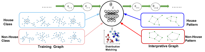
Figure 1: Overview of the proposed in-process global interpretation method GDM

Furthermore, by plugging the distribution matching objective Eq. (3) into Eq. (2), and generating interpretive graphs for multiple class simultaneously $\mathcal{S}=\{\mathcal{S}_{c}\}^{C}_{c=1}$, we can rewrite our learning goal as follows:

$$\min_{\mathcal{S}}\ \underset{\bm{\theta}_{0}\sim P_{\bm{\theta}_{0}}}{\mathbb{E}}\left[\underset{t\sim\mathcal{T}}{\mathbb{E}}\big{[}\sum_{c=1}^{C}\mathcal{L}_{\text{DM}}(f_{\bm{\theta}_{t}}(\mathcal{S}_{c}))\big{]}\right] \text{s.t.\ }\bm{\theta}_{t},\bm{\psi}_{t}=\mathtt{opt-alg}_{\bm{\theta},\bm{\psi}}(\mathcal{L}_{\text{CE}}(h_{\bm{\psi}_{t-1}},f_{\bm{\theta}_{t-1}}),\varsigma)$$ (5)

The interpretation procedure is based on the parameter trajectory of the model, while the training procedure on the original classification task is independently done. Thus this method can serve as a plug-in without influencing normal model training. In order to learn interpretive graphs that generalize to a distribution of model initializations $P_{\bm{\theta}_{0}}$, we can sample $\bm{\theta}_{0}\sim P_{\bm{\theta}_{0}}$ to obtain multiple trajectories.

3.5 Practical Constraints in Graph Optimization

Optimizing each interpretive graph is essentially optimizing its adjacency matrix and node feature. Denote a interpretive graph as $S=(\textbf{A}_{s},\textbf{X}_{s})$, with $\textbf{A}_{s}\in\{0,1\}^{m\times m}$ and $\textbf{X}_{s}\in\mathbb{R}^{m\times d}$. To generate solid graph explanations using Eq. (5), we introduce several practical constraints on $\textbf{A}_{s}$ and $\textbf{X}_{s}$. The constraints are applied on each interpretive graph, concerning discrete graph structure, matching edge sparsity, and feature distribution with the training data.

Discrete Graph Structure Optimizing the adjacency matrix is challenging as it has discrete values. To address this issue, we assume that each entry in matrix $\textbf{A}_{s}$ follows a Bernoulli distribution $\mathcal{B}(\Omega):p(\textbf{A}_{s})=\textbf{A}_{s}\odot\sigma(\Omega)+(1-\textbf{A}_{s})\odot\sigma(-\Omega)$, where $\Omega\in[0,1]^{m\times m}$ is the Bernoulli parameters, $\sigma(\cdot)$ is element-wise sigmoid function and $\odot$ is the element-wise product, following [12, 17, 16]. Therefore, the optimization on $\textbf{A}_{s}$ involves optimizing $\Omega$ and then sampling from the Bernoulli distribution. However, the sampling operation is non-differentiable, thus we employ the reparameterization method [20] to refactor the discrete random variable into a function of a new variable $\varepsilon\sim\text{Uniform}(0,1)$. The adjacency matrix can then be defined as a function of Bernoulli parameters as follows, which is differentiable w.r.t. $\Omega$:

$$\textbf{A}_{s}(\Omega)=\sigma((\log\varepsilon-\log(1-\varepsilon)+\Omega)/\tau),$$ (6)

where $\tau\in(0,\infty)$ is the temperature parameter that controls the strength of continuous relaxation: as $\tau\rightarrow 0$, the variable $\textbf{A}_{s}$ approaches the Bernoulli distribution. Now Eq. (6) turns the problem of optimizing the discrete adjacency matrix $\textbf{A}_{s}$ into optimizing the Bernoulli parameter matrix $\Omega$.

Matching Edge Sparsity Our interpretive graphs are initialized by randomly sampling subgraphs from training graphs, and their adjacency matrices will be freely optimized, which might result in too sparse or too dense graphs. To prevent such scenarios, we exert a sparsity matching loss by penalizing the distance of sparsity between the interpretive and the training graphs, following [12]:

$$\mathcal{L}_{\text{sparsity}}(\mathcal{S})=\sum_{(\textbf{A}_{s}(\Omega),\textbf{X}_{s})\sim\mathcal{S}}\max(\bar{\Omega}-\epsilon,0),$$ (7)

where $\bar{\Omega}=\sum_{ij}\sigma(\Omega_{ij})/|\Omega|$ calculates the expected sparsity of a interpretive graph, and $\epsilon$ is the average sparsity of initialized $\sigma(\Omega)$ for all interpretive graphs, which are sampled from original training graphs thus resembles the sparsity of training dataset.

Matching Feature Distribution Real graphs in practice may have skewed feature distribution; without constraining the feature distribution on interpretive graphs, rare features might be overshadowed by the dominating ones. For example, in the molecule dataset MUTAG, node feature is the atom type, and certain node types such as Carbons dominate the whole graphs. Therefore, when optimizing the feature matrix of interpretive graphs for such unbalanced data, it is possible that only dominating node types are maintained. To alleviate this issue, we propose to match the feature distribution between the training graphs and the interpretive ones.

Specifically, for each graph $G=(\textbf{A, X})$ with $n$ nodes, we estimate the graph-level feature distribution as $\bar{\textbf{x}}=\sum^{n}_{i=1}\textbf{X}_{i}/n\in{\mathbb{R}^{d}}$, which is essentially a mean pool of the node features. For each class $c$, we then define the following feature matching loss:

$$\mathcal{L}_{\text{feat}}(\mathcal{S}_{c})=\|\frac{1}{|\mathcal{G}_{c}|}\sum_{(\textbf{A, X})\in\mathcal{G}_{c}}\bar{\textbf{x}}-\frac{1}{|\mathcal{S}_{c}|}\sum_{(\textbf{A}_{s},\textbf{X}_{s})\in\mathcal{S}_{c}}\bar{\textbf{x}}_{s}\|^{2},$$ (8)

where we empirically measure the class-level feature distribution by calculating the average of graph-level features. By minimizing the feature distribution distance in Eq. (8), even rare features can have a chance to be distilled in the interpretive graphs.

3.6 Final Objective and Algorithm

Integrating the practical constraints discussed in Section 3.5 with the distribution matching based in-process interpretation framework in Eq. (5) in Section 6.8, we now obtain the final objective for optimizing the interpretive graphs, which essentially is determined by the Bernoulli parameters for sampling discrete adjacency matrices and the node feature matrices. Formally, we propose Graph Distribution Matching (GDM), which aims to solve the following optimization problem:

$$\min_{\mathcal{S}}\ \underset{\bm{\theta}_{0}\sim P_{\bm{\theta}_{0}}}{\mathbb{E}}\left[\underset{t\sim\mathcal{T}}{\mathbb{E}}\big{[}\sum_{c=1}^{C}\mathcal{L}_{\text{DM}}(f_{\bm{\theta}_{t}}(\mathcal{S}_{c}))+\alpha\cdot\mathcal{L}_{\text{feat}}(\mathcal{S}_{c})+\beta\cdot\mathcal{L}_{\text{sparsity}}(\mathcal{S})\big{]}\right]$$

$$\text{s.t.\ }\bm{\theta}_{t},\bm{\psi}_{t}=\mathtt{opt-alg}_{\bm{\theta},\bm{\psi}}(\mathcal{L}_{\text{CE}}(h_{\bm{\psi}_{t-1}},f_{\bm{\theta}_{t-1}}),\varsigma)$$ (9)

where we use $\alpha$ and $\beta$ to control the strength of regularizations on feature distribution matching and edge sparsity respectively. We explore the sensitivity of hyper-parameters $\alpha$ and $\beta$ in Appendix 6.6. Detailed algorithm of our proposed GDM is provided in Appendix 6.1.

Complexity Analysis We now analyze the time complexity of the proposed method. Suppose for each iteration, we sample $B_{1}$ interpretive graphs and $B_{2}$ training graphs, and their average node number is $n$. The inner loop for interpretive graph update takes $n(B_{1}+B_{2})$ computations on node, while the update of GNN model uses $nB_{2}$ computations. Therefore the overall complexity is $\mathcal{O}(nKT(B_{1}+2B_{2}))$, which is of the same magnitude of complexity for normal GNN training. This demonstrates the efficiency of our interpretation method: it can simultaneously generate interpretations as the training of GNN model proceeds, without introducing extra complexity.

4 Experimental Studies

4.1 Experimental Setup

Dataset The interpretation performance is evaluated on the following synthetic and real-world datasets for graph classification, whose statistics can be found in Appendix 6.2.

• Real-world data includes: MUTAG, which contains chemical compounds where nodes are atoms and edges are chemical bonds. Each graph is labeled as whether it has a mutagenic effect on a bacterium [3]. Graph-Twitter [24] includes Twitter comments for sentiment classification with three classes. Each comment sequence is presented as a graph, with word embedding as node feature. Graph-SST5 [35] is a similar dataset with reviews, where each review is converted to a graph labeled by one of five rating classes.

• Synthetic data includes: Shape contains four classes of graphs: Lollipop, Wheel, Grid, and Star. For each class, we synthesize the same number of graphs with a random number of nodes using NetworkX [10]. BA-Motif [19] uses Barabasi-Albert (BA) graph as base graphs, among which half graphs are attached with a “house” motif and the rest with “non-house” motifs. BA-LRP [23] based on Barabasi-Albert (BA) graph includes one class being node-degree concentrated graphs, and the other degree-evenly graphs. These datasets do not have node features, thus we use node index as the surrogate feature.

Baseline Note that this work is the first in-process global interpretation method for graph learning, thus no directly comparable baseline exists. However, we can still compare GDM with different types of works from multiple perspectives to demonstrate its advantages:

• GDM versus post-hoc interpretation baselines: This comparison aims to verify the necessity of leveraging in-process training trajectory for accurate global interpretation, compared with post-hoc global interpretation methods [34, 28]. We compare GDM with XGNN [34], which is the only open-sourced post-hoc global interpretation method for graph learning; XGNN heavily relies on domain knowledge (e.g. chemical rules), thus it is only adopted on MUTAG. We further consider GDM-final, which is a variant of GDM that generates interpretations only based on the final-step model snapshot, instead of the in-process training trajectory. We also include a simple Random strategy as a reference, which randomly selects graphs from the training set as interpretations.

• GDM versus local interpretation baselines: This comparison is to demonstrate the effectiveness of global interpretation with only few interpretive graphs generated for each class, compared with existing local interpretation works generating interpretation per graph instance. Note that most existing local interpretation solutions [31, 21, 1] are post-hoc and evaluated on test instances, here we generate their interpretations of a pre-trained GNN on training instances for a fair knowledge availability. Detailed results can be found in Appendix 6.4.

• GDM versus inherently global-interpretable baseline: This comparison is to demonstrate that our general recipe of in-process interpretation can achieve better trade-off of model prediction and interpretation performance than simple inherently global-interpretable methods. The results and discussion are provided in Appendix 6.3.

Evaluation Protocol We comprehend interpretability from two perspectives, i.e., the interpretation should maintain utility to train a model and fidelity to be predicted as the right classes. Therefore, we establish the following evaluation protocols accordingly:

• Utility aims to verify whether generated interpretations can be utilized and leads to a well-trained GNN. Desired interpretations should capture the dominating patterns that guide the training procedure. For this protocol, we use the interpretive graphs to train a GNN model from scratch and report its performance on the test set. We call this accuracy utility.

• Fidelity is to validate whether the interpretation really captures discriminative patterns. Ideal interpretive graphs should be correctly classified to their corresponding classes by the trained GNN. In this protocol, given the trained GNN model, we report its prediction accuracy on the interpretive graphs. We define this accuracy as Fidelity.

Configurations We choose the graph convolution network (GCN) as the target GNN model for interpretation, as it is widely used for graph learning. It contain 3 layers with 256 hidden dimension, concatenated by a mean pooling layer and a dense layers in the end. Adam optimizer [13] is adopted for model training. In both evaluation protocols, we split the dataset as $85\%$ training and $15\%$ test data, and only use the training set to generate interpretative graphs. Given the interpretative graphs, each evaluation experiments are run $5$ times, with the mean and variance reported.

Table 1: Utility with a varying number of interpretive graphs generated per class.

Graphs/Cls	Graph-Twitter			Graph-SST5
	GDM	GDM-final	Random	GDM	GDM-final	Random
10	56.43 $\pm$ 1.39	41.69 $\pm$ 2.61	52.40 $\pm$ 0.29	35.72 $\pm$ 0.65	29.03 $\pm$ 0.79	21.07 $\pm$ 0.60
50	58.93 $\pm$ 1.29	54.80 $\pm$ 1.13	52.92 $\pm$ 0.27	43.81 $\pm$ 0.86	38.37 $\pm$ 0.71	23.15 $\pm$ 0.35
100	59.51 $\pm$ 0.31	57.39 $\pm$ 1.29	55.47 $\pm$ 0.51	44.43 $\pm$ 0.45	42.27 $\pm$ 0.17	25.26 $\pm$ 0.75
	GCN Accuracy:61.40			GCN Accuracy:44.39
	BA-Motif			BA-LRP
	GDM	GDM-final	Random	GDM	GDM-final	Random
1	71.66 $\pm$ 2.49	65.33 $\pm$ 7.31	67.60 $\pm$ 4.52	71.56 $\pm$ 3.62	68.81 $\pm$ 4.46	77.48 $\pm$ 1.21
5	96.00 $\pm$ 1.63	91.33 $\pm$ 2.05	77.60 $\pm$ 2.21	91.60 $\pm$ 1.57	90.20 $\pm$ 1.66	77.76 $\pm$ 0.52
10	98.00 $\pm$ 0.00	89.33 $\pm$ 3.86	84.33 $\pm$ 2.49	94.90 $\pm$ 1.09	93.26 $\pm$ 0.83	88.38 $\pm$ 1.40
	GCN Accuracy: 100.00			GCN Accuracy: 97.95
	MUTAG			Shape
	GDM	GDM-final	Random	GDM	GDM-final	Random
1	71.92 $\pm$ 2.48	65.33 $\pm$ 7.31	50.87$\pm$ 15.0	93.33 $\pm$ 4.71	60.00 $\pm$ 8.16	33.20 $\pm$ 4.71
5	77.19 $\pm$ 4.96	73.68 $\pm$ 0.00	80.70 $\pm$ 2.40	96.66 $\pm$ 4.71	66.67 $\pm$ 4.71	85.39 $\pm$ 12.47
10	82.45 $\pm$ 2.48	73.68 $\pm$ 0.00	75.43 $\pm$ 6.56	100.00 $\pm$ 0.00	70.00 $\pm$ 8.16	87.36 $\pm$ 4.71
	GCN Accuracy:88.63			GCN Accuracy:100.00

4.2 Quantitative Analysis

Our major contribution is to incorporate the training trajectory for in-process interpretation, therefore, the main quantitative analysis aims to answer the following questions: 1) Is the in-process training trajectory necessary? 2) Is our in-process interpretation efficient compared with post-hoc method? To demonstrate the necessity of training trajectory, we compare GDM with post-hoc global interpretation baselines, XGNN, GDM-final, which provide global interpretation only using the final-step model.

Utility Performance In Table 1, we summarize the utility performance when generating different numbers of interpretive graphs per class, along with the benchmark GCN test accuracy for each dataset. Presumably, an ideal utility score should be comparable to the benchmark GCN accuracy when the model is trained on the original training set. We observe that the GCN model trained on GDM’s interpretive graphs can achieve remarkably higher utility score, compared with the post-hoc GDM-final baselines and the random strategy. Note that XGNN on MUTAG can only achieve a similar utility score as the random strategy, thus is excluded in the table. The comparison between GDM and GDM-final validates that the in-process training trajectory does help for capturing more informative patterns the model uses for training. Meanwhile, GDM-final could result in large variance on BA-Motif and Shape, which reflects the instability of post-hoc methods.

Fidelity Performance In Table 2, we compare GDM and GDM-final in terms of the fidelity of generated interpretive graphs. We observe that GDM achieves over $90\%$ fidelity score on all datasets, which indicates that GDM indeed captures discriminative patterns. Though being slightly worse than XGNN on MUTAG, GDM achieves much better utility. Meanwhile, different from XGNN, we do not include any dataset specific rules, thus is a more general interpretation solution.

Table 2: Fidelity and Efficiency when generating 10 interpretive graphs per class.

width=center Dataset Graph-Twitter Graph-SST5 BA-Motif BA-LRP Shape MUTAG XGNN on MUTAG GDM-final 93.20$\pm$ 0.00 88.60 $\pm$ 0.09 68.30 $\pm$ 0.02 98.20 $\pm$ 0.02 100.00$\pm$ 0.00 66.60 $\pm$ 0.02 100.00$\pm$ 0.00 GDM 94.44$\pm$ 0.015 90.67$\pm$ 0.019 95.00$\pm$ 1.11 96.67$\pm$ 0.023 100.00$\pm$ 0.00 96.67 $\pm$ 0.045 Time (s) 129.63 327.60 108.00 110.43 210.52 218.45 838.20

Efficiency Another advantage of GDM is that it generates interpretations in an efficient manner. As shown in Table 2, GDM is almost 4 times faster than the post-hoc global interpretation method XGNN. Our methods takes almost no extra cost to generate multiple interpretative graphs, as there are only few interpretive graphs compared with the training dataset. XGNN, however, select each edge in each graph by a reinforcement learning policy which makes the interpretation process rather expensive. We also explore an accelerated version for GDM in Appendix 6.7.

4.3 Qualitative Analysis

width=center Dataset Real Graph Global Interpretation Real Graph Global Interpretation House Class Non-House Class BA-Motif Wheel Class Lollipop Class Shape Grid Class Star Class

Table 3: Visualization of real example graphs and generated global interpretations.

We qualitatively visualize the global interpretations provided by GDM to verify that GDM can capture human-intelligible patterns, which indeed correspond to the ground-truth rules for discriminating classes. Table 3 shows examples in BA-Motif and Shape datasets, and more results and analyses on other datasets can be found in Appendix 6.9.

The qualitative results show that the global explanations successfully identify the discriminative patterns for each class. If we look at BA-Motif dataset, for the house-shape class, the interpretation has captured such a pattern of house structure, regardless of the complicated base BA graph in the other part of graphs; while in the non-house class with five-node cycle, the interpretation also successfully grasped it from the whole BA-Motif graph. Regarding the Shape dataset, the global interpretations for all the classes are almost consistent with the ground-truth graph patterns, i.e., Wheel, Lollipop, Grid and Star shapes are also reflected in the interpretation graphs. Note that the difference for interpretative graphs of Star and Wheel are small, which provides a potential explanation for our fidelity results in Table 2, where pre-trained GNN models cannot always distinguish interpretative graphs of Wheel shape with interpretative graphs of Star shape.

5 Conclusions

In this work, we studied a new problem to enhance interpretability for graph learning: how to achieve in-process global interpretation to understand the high-level patterns the model learns during training? We proposed a novel framework, where interpretations are optimized based on the whole training trajectory. We designed an interpretation method GDM via distribution matching, which matches the embeddings generated by the GNN model for the training data and interpretive data. Our framework can generate an arbitrary number of interpretable and effective interpretive graphs. Our study puts the first step toward in-process global interpretation and offers a comprehensive understanding of GNNs. We evaluated our method both quantitatively and qualitatively on real-world and interpretive datasets, and the results indicate that the explanation graphs produced by GDM achieve high performance and be able to capture class-relevant structures and demonstrate efficiency. One possible limitation of our work is that the interpretations are a general summarizing of the whole training procedure, thus cannot reflect the dynamic change of the knowledge captured by the model to help early detect anomalous behavior, which we believe is an important and challenging open problem. In the future work, we aim to extend the proposed framework to study model training dynamics.

6 Appendix

6.1 GDM Algorithm

To solve the final objective in Eq. (9), we use mini-batch based training procedure as depicted in Algorithm 1. We first initialize all the explanation graphs by sampling sub-graphs from the training graphs, with node number being set as the average node number of training graphs for the corresponding class. The GNN model can be randomly initialized for $K$ times. For each randomly initialized GNN model, we train it for $T$ iterations. During each iteration, we sample a mini-batch of training graphs and explanation graphs. We first apply one step of update for explanation graphs based on the current GNN feature extractor; then update the GNN model for one step using normal graph classification loss.

Algorithm 1 GDM: Learning Explanation Graphs

1:Input: Training data $\mathcal{G}=\{\mathcal{G}_{c}\}^{C}_{c=1}$

2:Initialize explanation graphs $\mathcal{S}=\{\mathcal{S}_{c}\}_{c=1}^{C}$ for each class $c$

3:for $k=0,\dots,K-1$ do

4:     Initialize GNN by sampling $\bm{\theta}_{0}\sim P_{\bm{\theta}},\bm{\psi}_{0}\sim P_{\bm{\psi}}$

5:     for $t=0,\ldots,T-1$ do

6:         Sample mini-batch graphs $B^{\mathcal{S}}=\{B_{c}^{\mathcal{S}}\sim\mathcal{S}_{c}\}^{C}_{c=1}$

7:         Sample mini-batch graphs $B^{\mathcal{G}}=\{B_{c}^{\mathcal{G}}\sim\mathcal{G}_{c}\}^{C}_{c=1}$

8:         # Optimize global interpretive graphs

9:         for class $c=1,\dots,C$ do

10:              Compute the interpretation loss following Eq. (9): $\mathcal{L}_{c}=\mathcal{L}_{\text{DM}}(f_{\bm{\theta}_{t}}(B_{c}^{\mathcal{S}}))+\alpha\cdot\mathcal{L}_{\text{feat}}(B^{\mathcal{S}}_{c})+\beta\cdot\mathcal{L}_{\text{sparsity}}(B^{\mathcal{S}}_{c})$

11:         end for

12:         Update explanation graphs $\mathcal{S}\leftarrow\mathcal{S}-\eta\nabla_{\mathcal{S}}\sum_{c=1}^{C}\mathcal{L}_{c}$

13:         # Optimize GNN model as normal

14:         Compute normal training loss for graph classification task $\mathcal{L}_{\text{CE}}(h_{\bm{\psi}_{t-1}},f_{\bm{\theta}_{t-1}})=\sum_{G\sim B^{\mathcal{G}}}\mathscr{l}(h_{\bm{\psi}_{t-1}}(f_{\bm{\theta}_{t-1}}(G)),y)$

15:         Update $\bm{\theta}_{t+1}=\bm{\theta}_{t}-\eta_{1}\nabla_{\bm{\theta}}\mathcal{L}_{\text{CE}}(h_{\bm{\psi}_{t-1}},f_{\bm{\theta}_{t-1}})$

16:         Update $\bm{\psi}_{t+1}=\bm{\psi}_{t}-\eta_{2}\nabla_{\bm{\psi}}\mathcal{L}_{\text{CE}}(h_{\bm{\psi}_{t-1}},f_{\bm{\psi}_{t-1}})$

17:     end for

18:end for

19:Output: Explanation graphs $\mathcal{S}^{*}=\{\mathcal{S}^{*}_{c}\}_{c=1}^{C}$ for each class $c$

6.2 Dataset Statistics

The data statistics on both synthetic and real-world datasets for graph classification are provided in Table 4. The ground-truth performance of GCN model is also listed for reference.

Table 4: Basic Graph Statistics

Dataset	BA-Motif	BA-LRP	Shape	MUTAG	Graph-Twitter	Graph-SST5
# of classes	2	2	4	2	3	5
# of graphs	1000	20000	100	188	4998	8544
Avg. # of nodes	25	20	53.39	17.93	21.10	19.85
Avg. # of edge	50.93	42.04	813.93	19.79	40.28	37.78
GCN Accuracy	100.00	97.95	100.00	88.63	61.40	44.39

6.3 GDM versus Inherently Global-Interpretable Model

We compare the performance of GDM with a simple yet inherently global-interpretable method, logistic regression with hand-crafted graph-based features. When performing LR on these graph-structured data, we leverage the Laplacian matrix as graph features: we first sort row/column of adjacency matrix by nodes’ degree to align the feature dimensions across different graphs; we then flatten the reordered laplacian matrix as input for LR model. When generating interpretations, we first train a LR on training graphs and obtain interpretations as the top most important features (i.e. edges on graph) based on regression weights where average number of edges. We then report the utility of LR interpretations, shown in the following table 5.

Table 5: Utility of Logistic Regression

Dataset	MUTAG	BA-Motif	BA-LRP	Shape	Graph-Twitter	Graph-SST5
LR Interpretation	93.33%	100%	100%	100%	42.10%	22.68%
Original LR	96.66%	100%	100%	100%	52.06%	27.45%

Table 6: Utility of GDM on large datasets

# of interpretive graphs per class	Graph-Twitter	Graph-SST5
10	56.43 $\pm$ 1.39	40.30 $\pm$ 1.27
50	58.93 $\pm$ 1.29	42.70 $\pm$ 1.10
100	59.51 $\pm$ 0.31	44.37 $\pm$ 0.28
Original GCN Accuracy	61.40	44.39

LR shows good interpretation utility on simple datasets like BA-Motif and BA-LRP, but it has much worse performance on more sophisticated datasets, compared with GDM in table 6. For example, interpretations generated by GDM can achieve close accuracy as the original GCN model.

6.4 GDM versus Local Interpretation

As aforementioned, GDM provides global interpretation, which is significantly different from the extensively studied local interpretation methods: we only generate few small interpretive graphs per class to reflect the high-level discriminative patterns the model captures; while local interpretation is for each graph instance. Though our global interpretation is not directly comparable with existing local interpretation, we still compare their interpretation utility to demonstrate the efficacy of our GDM when we only generate a few interpretive graphs. The results can be found in Table 7. We compare our model with GNNExplainer,PGExplainer and Captum on utility. For Graph-SST5 and Graph-Twitter, we generate 100 graphs for each class and 10 graphs for other datasets.

Table 7: Utility Compared with Local Interpretation

Datasets	Graph-SST5	Graph-Twitter	MUTAG	BA-Motif	Shape	BA-LRP
GDM	44.43 $\pm$0.45	59.51 $\pm$ 0.31	82.45$\pm$2 .48	98.00$\pm$0.00	100 $\pm$0.00	94.90$\pm$1.09
GNNExplainer	43.00$\pm$0.07	58.12$\pm$1.48	73.68$\pm$5.31	93.2$\pm$0.89	89.00$\pm$4.89	58.65$\pm$4.78
PGExplainer	28.41 $\pm$ 0.00	55.46 $\pm$ 0.03	75.62$\pm$4.68	62.58$\pm$0.66	71.75$\pm$1.85	50.25$\pm$0.15
Captum	28.83$\pm$0.05	55.76$\pm$0.42	89.20$\pm$0.01	52.00$\pm$0.60	80.00$\pm$0.01	49.25$\pm$0.01

Comparing these results, we can observe that the GDM obtains higher utility score compared to different GNN explaination methods, with relatively small variance.

6.5 One Use Case of In-Process Interpretation

A use case of in-process interpretation is when the queried data is very different from the data used to train the model (i.e. out-of-distribution): fidelity score could fail to reflect intrinsic patterns learned by the model, as post-hoc interpretation also heavily relies on the property of queried data; and post-hoc methods are usually used when only given the pre-trained model without knowing the training data (the scenario when training data is provided can be found in Appendix 6.4). In contrast, our in-process interpretation is generated during model training without accessing any auxiliary data, and thus is free of influence from the quality of queried data.

To mimic such a out-of-distribution case, we conduct a post-hoc interpretation experiment where the GCN model is trained on BA-LRP, and is used on BA-Motif. We use PGExplainer as an example post-hoc (local) interpretation method. The post-hoc interpretation utility is shown below when training and test data are from the same or different distribution.

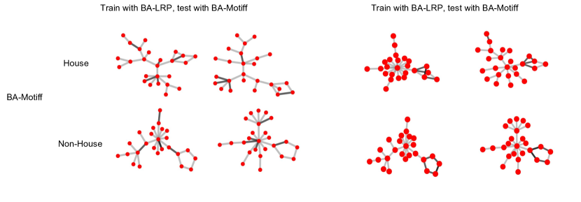
Figure 2: Performance of PGExplainer under Out-of-distribution Scenario

Table 8: PGExplainer interpretation utility

Scenario	Training Data	Test Data	Utility $\pm$ std
Same Distribution	BA-Motif	BA-Motif	80.11 $\pm$ 0.08
Out of Distribution	BA-LRP	BA-Motif	75.34 $\pm$ 0.16

As we expected, the utility drops 5%. Meanwhile, we provide a visualization of generated interpretation via 2 where we can see that PGExplainer fails to capture the most important motif in BA-Motif graphs (i.e. house/non-house subgraph). This case study demonstrates that post-hoc methods cannot provide valid interpretations under distribution shifts. In contrast, in-process interpretation is generated along with model training and does not rely on what instances are queried post-hoc. The out-of-distribution case could be popular in real-world scenarios, and in-process interpretation is a complementary tool for model interpretability when post-hoc interpretability is not possible/suitable.

6.6 Hyperparameter Analysis

In our final objective Eq. (9), we defined two hyper-parameters $\alpha$ and $\beta$ to control the strength for feature matching and sparsity matching regularization, respectively.

In this subsection, we explore the sensitivity of hyper-parameters $\alpha$ and $\beta$. Since MUTAG is the only dataset that contains node features, we only apply the feature matching regularization on this dataset. We report the in-process utility with different feature-matching coefficients $\alpha$ in Table 9. A larger $\alpha$ means we have a stronger restriction on the node feature distribution. We found that when we have more strict restrictions, the utility increases slightly. This is an expected behavior since the node features from the original MUTAG graphs contain rich information for classifications, and matching the feature distribution enables the interpretation to capture rare node types. By having such restrictions, we successfully keep the important feature information in our interpretive graphs.

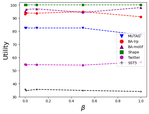
Figure 3: Sensitivity analysis of hyper-parameter $\beta$ for the sparsity matching regularization

Moreover, we vary the sparsity coefficient $\beta$ in the range of $\{0.001,0.01,0.1,0.5,1\}$, and report the utility for all of our four datasets in Figure 3. For most datasets excluding Shape, the performance start to degrade when the $\beta$ becomes larger than 0.5. This means that when the interpretive graph becomes more sparse, it will lose some information during training time.

Table 9: Sensitivity analysis of hyper-parameter $\alpha$ for feature matching regularization.

$\alpha$	0.005	0.01	0.05	0.5	1.0
Utility	82.45	82.45	82.45	82.45	80.70

6.7 Special Case of Our Framework

We also explore a special case when the GNN model is not updated when generating explanations, as discussed in Section 3.6. For this case, we randomly initialized different GNNs in each iteration with parameters fixed within each iteration as shown in algorithm 2 To our surprise, the generated graphs are also quite effective in training a well-performed GNN. As shown in Table 10, the interpretation utility of our methods does not degrade when the explanations are optimized without updating the GNN model in each iteration. This indicates that randomly initialized GNNs are already able to produce informative interpretation patterns. This finding echoes the observations from previous work in image classification [2] and node classification [26]. They have shown a similar observation that random neural networks can generate powerful representations, and random networks can perform a distance-preserving embedding of the data to make smaller distances between samples of the same class [8]. Our finding further verifies such a property also stands for GNNs on the graph classification task from the perspective of model interpretation.

Table 10: Utility without updating GCN.

Graphs/Cls	BA-Motif	BA-LRP	Shape	MUTAG
1	83.12 $\pm$ 2.16	79.95 $\pm$ 3.50	70.00 $\pm$ 21.60	71.93 $\pm$ 8.94
5	99.33 $\pm$ 0.47	88.46 $\pm$ 1.11	100.00 $\pm$ 0.00	89.47 $\pm$ 7.44
10	100.00 $\pm$ 0.00	93.53 $\pm$ 3.41	100.00 $\pm$ 0.00	85.96 $\pm$ 2.48
Graphs/Cls	Graph-Twitter		Graph-SST5
10	52.97 $\pm$ 0.29		40.30 $\pm$ 1.27
50	57.63 $\pm$ 0.92		42.70 $\pm$ 1.10
100	58.35 $\pm$ 1.32		44.37 $\pm$ 0.28

Algorithm 2 GDM without GNN training

1:Input: Training data $\mathcal{G}=\{\mathcal{G}_{c}\}^{C}_{c=1}$

2:Initialize explanation graphs $\mathcal{S}=\{\mathcal{S}_{c}\}_{c=1}^{C}$ for each class $c$

3:for $k=0,\dots,K-1$ do

4:     Initialize GNN by sampling $\bm{\theta}_{0}\sim P_{\bm{\theta}},\bm{\psi}_{0}\sim P_{\bm{\psi}}$

5:     for $t=0,\ldots,T-1$ do

6:         Sample mini-batch graphs $B^{\mathcal{S}}=\{B_{c}^{\mathcal{S}}\sim\mathcal{S}_{c}\}^{C}_{c=1}$

7:         Sample mini-batch graphs $B^{\mathcal{G}}=\{B_{c}^{\mathcal{G}}\sim\mathcal{G}_{c}\}^{C}_{c=1}$

8:         for class $c=1,\dots,C$ do

9:              Compute the interpretation loss:

10:$\mathcal{L}_{c}=\mathcal{L}_{\text{DM}}(f_{\bm{\theta}_{L}}(B_{c}^{\mathcal{S}}))+\alpha\cdot\mathcal{L}_{\text{feat}}(B^{\mathcal{S}}_{c})+\beta\cdot\mathcal{L}_{\text{sparsity}}(B^{\mathcal{S}}_{c})$

11:         end for

12:         Update explanation graphs $\mathcal{S}\leftarrow\mathcal{S}-\eta\nabla_{\mathcal{S}}\sum_{c=1}^{C}\mathcal{L}_{c}$

13:     end for

14:end for

15:Output: Explanation graphs $\mathcal{S}^{*}=\{\mathcal{S}^{*}_{c}\}_{c=1}^{C}$ for each class $c$

6.8 Gain of Distribution Matching

We construct an ablation method that adopts Algorithm 1 but replaces the design of matching embedding by matching the output probability distribution in the label space instead. The in-process utility of such a label-matching baseline is as follows in table 11:

Table 11: Utility comparison, with a varying number of explanation graphs generated per class.

Graphs/Cls	Graph-Twitter			Graph-SST5
	GDM	GDM-label	Random	GDM	GDM-label	Random
10	56.43 $\pm$ 1.39	40.00 $\pm$ 3.98	52.40 $\pm$ 0.29	35.72 $\pm$ 0.65	25.49 $\pm$ 0.39	24.90 $\pm$ 0.60
50	58.93 $\pm$ 1.29	55.62 $\pm$ 1.12	52.92 $\pm$ 0.27	43.81 $\pm$ 0.86	31.47 $\pm$ 2.58	23.15 $\pm$ 0.35
100	59.51 $\pm$ 0.31	53.37 $\pm$ 0.55	55.47 $\pm$ 0.51	44.43 $\pm$ 0.45	32.01 $\pm$ 1.90	25.26 $\pm$ 0.75
	BA-Motif			BA-LRP
	GDM	GDM-label	Random	GDM	GDM-label	Random
1	71.66 $\pm$ 2.49	50.63 $\pm$ 0.42	67.60 $\pm$ 4.52	71.56 $\pm$ 3.62	54.11 $\pm$ 5.33	77.48 $\pm$ 1.21
5	96.00 $\pm$ 1.63	82.54 $\pm$ 0.87	77.60 $\pm$ 2.21	91.60 $\pm$ 1.57	59.21 $\pm$ 0.99	77.76 $\pm$ 0.52
10	98.00 $\pm$ 0.00	90.89 $\pm$ 0.22	84.33 $\pm$ 2.49	94.90 $\pm$ 1.09	66.40 $\pm$ 1.47	88.38 $\pm$ 1.40
	MUTAG			Shape
	GDM	GDM-label	Random	GDM	GDM-label	Random
1	71.92 $\pm$ 2.48	70.17 $\pm$ 2.48	50.87$\pm$ 15.0	93.33 $\pm$ 4.71	60.00 $\pm$ 7.49	33.20 $\pm$ 4.71
5	77.19 $\pm$ 4.96	57.89 $\pm$ 4.29	80.70 $\pm$ 2.40	96.66 $\pm$ 4.71	85.67 $\pm$ 2.45	85.39 $\pm$ 12.47
10	82.45 $\pm$ 2.48	59.65 $\pm$ 8.94	75.43 $\pm$ 6.56	100.00 $\pm$ 0.00	88.67 $\pm$ 4.61	87.36 $\pm$ 4.71

Comparing these results, we can observe that the distribution matching design is effective: disabling this design will greatly deteriorate the performance.

6.9 More Qualitative Results

MUTAG This dataset has two classes: “non-mutagenic” and “mutagenic”. As discussed in previous works [3, 31], Carbon rings along with $NO_{2}$ chemical groups are known to be mutagenic. And [19] observe that Carbon rings exist in both mutagen and non-mutagenic graphs, thus are not really discriminative. Our synthesized interpretive graphs are also consistent with these “ground-truth” chemical rules. For ‘mutagenic” class, we observe two $NO_{2}$ chemical groups within one interpretative graph, and one $NO_{2}$ chemical group and one carbon ring, or multiple carbon rings from a interpretative graph. For the class of “non-mutagenic”, we observe that $NO_{2}$ groups exist much less frequently but other atoms, such as Chlorine, Bromine, and Fluorine, appear more frequently. To visualize the structure more clearly, we limit the max number of nodes to 15 such that we do not have too complicate interpretative graphs.

BA-Motif and BA-LRP The qualitative results on BA-Motif dataset show that the explanations for all classes successfully identify the discriminative features. For House-shape class, all the generated graphs have captured such a pattern of house structure, regardless of the complicated base BA graph in the other part of graphs. For the other class with five-node cycle, our generated graphs successfully grasp it from the whole BA-Motif graph. In BA-LRP dataset, the first class consists of Barabasi-Albert graphs of growth parameter 1, which means new nodes attached preferably to low degree nodes, while the second class has new nodes attached to Barabasi-Albert graphs preferably to higher degree nodes. Our interpretative dataset again correctly identify discriminative patterns to differentiate these two classes, which are the tree-shape and ring-shape structures.

Shape In Table 12, the generated explanation graphs for all the classes are almost consistent with the desired graph patterns. Note that the difference for interpretative graphs of Star and Wheel are small. This provides a potential explanation for our post-hoc quantitative results in Table 1, where pre-trained GNN models cannot always distinguish interpretative graphs of Wheel shape with interpretative graphs of Star shape.

Dataset	Class	Training Graph Example	Synthesized Interpretation Graph
BA-Motif	House
	Non-House
BA-LRP	Low Degree
	High Degree
MUTAG	Mutagenicity
	Non-Mutagenicity
Shape	Wheel
	Lollipop
	Grid
	Star

Table 12: The qualitative results for all datasets. For each class in each dataset, as a reference, the example graph selected from the training data is displayed in the left column, while the generated explanation graphs are in the right column. Different node colors in MUTAG represent different node types.

References

- [1] Chirag Agarwal, Owen Queen, Himabindu Lakkaraju, and Marinka Zitnik. Evaluating explainability for graph neural networks. Scientific Data, 10(144), 2023.
- [2] Ehsan Amid, Rohan Anil, Wojciech Kotłowski, and Manfred K Warmuth. Learning from randomly initialized neural network features. arXiv preprint arXiv:2202.06438, 2022.
- [3] Asim Kumar Debnath, Rosa L Lopez de Compadre, Gargi Debnath, Alan J Shusterman, and Corwin Hansch. Structure-activity relationship of mutagenic aromatic and heteroaromatic nitro compounds. correlation with molecular orbital energies and hydrophobicity. Journal of medicinal chemistry, 34(2):786–797, 1991.
- [4] Mengnan Du, Ninghao Liu, and Xia Hu. Techniques for interpretable machine learning. Communications of the ACM, 63(1):68–77, 2019.
- [5] David Duvenaud, Dougal Maclaurin, Jorge Aguilera-Iparraguirre, Rafael Gómez-Bombarelli, Timothy Hirzel, Alán Aspuru-Guzik, and Ryan P. Adams. Convolutional networks on graphs for learning molecular fingerprints. In NeurIPS, 2015.
- [6] Lukas Faber, Amin K. Moghaddam, and Roger Wattenhofer. When comparing to ground truth is wrong: On evaluating gnn explanation methods. In Proceedings of the 27th ACM SIGKDD Conference on Knowledge Discovery & Data Mining, pages 332–341, 2021.
- [7] Justin Gilmer, Samuel S Schoenholz, Patrick F Riley, Oriol Vinyals, and George E Dahl. Neural message passing for quantum chemistry. In International conference on machine learning, pages 1263–1272. PMLR, 2017.
- [8] Raja Giryes, Guillermo Sapiro, and Alex M Bronstein. Deep neural networks with random gaussian weights: A universal classification strategy? IEEE Transactions on Signal Processing, 64(13):3444–3457, 2016.
- [9] Arthur Gretton, Karsten M Borgwardt, Malte J Rasch, Bernhard Schölkopf, and Alexander Smola. A kernel two-sample test. The Journal of Machine Learning Research, 13(1):723–773, 2012.
- [10] Aric Hagberg, Pieter Swart, and Daniel S Chult. Exploring network structure, dynamics, and function using networkx. Technical report, Los Alamos National Lab.(LANL), Los Alamos, NM (United States), 2008.
- [11] Qiang Huang, Makoto Yamada, Yuan Tian, Dinesh Singh, and Yi Chang. Graphlime: Local interpretable model explanations for graph neural networks. IEEE Transactions on Knowledge and Data Engineering, pages 1–6, 2022.
- [12] Wei Jin, Xianfeng Tang, Haoming Jiang, Zheng Li, Danqing Zhang, Jiliang Tang, and Bing Yin. Condensing graphs via one-step gradient matching. In Proceedings of the 28th ACM SIGKDD Conference on Knowledge Discovery and Data Mining, pages 720–730, 2022.
- [13] Diederik P Kingma and Jimmy Ba. Adam: A method for stochastic optimization. arXiv preprint arXiv:1412.6980, 2014.
- [14] Thomas N Kipf and Max Welling. Semi-supervised classification with graph convolutional networks. arXiv preprint arXiv:1609.02907, 2016.
- [15] Lu Lin, Ethan Blaser, and Hongning Wang. Graph embedding with hierarchical attentive membership. arXiv preprint arXiv:2111.00604, 2021.
- [16] Lu Lin, Ethan Blaser, and Hongning Wang. Graph structural attack by perturbing spectral distance. In Proceedings of the 28th ACM SIGKDD Conference on Knowledge Discovery and Data Mining, pages 989–998, 2022.
- [17] Lu Lin, Jinghui Chen, and Hongning Wang. Spectral augmentation for self-supervised learning on graphs. arXiv preprint arXiv:2210.00643, 2022.
- [18] Dongsheng Luo, Wei Cheng, Dongkuan Xu, Wenchao Yu, Bo Zong, Haifeng Chen, and Xiang Zhang. Parameterized explainer for graph neural network. Advances in neural information processing systems, 33:19620–19631, 2020.
- [19] Dongsheng Luo, Wei Cheng, Dongkuan Xu, Wenchao Yu, Bo Zong, Haifeng Chen, and Xiang Zhang. Parameterized explainer for graph neural network. Advances in neural information processing systems, 33:19620–19631, 2020.
- [20] Chris J Maddison, Andriy Mnih, and Yee Whye Teh. The concrete distribution: A continuous relaxation of discrete random variables. arXiv preprint arXiv:1611.00712, 2016.
- [21] Siqi Miao, Mia Liu, and Pan Li. Interpretable and generalizable graph learning via stochastic attention mechanism. In International Conference on Machine Learning, pages 15524–15543. PMLR, 2022.
- [22] Phillip E. Pope, Soheil Kolouri, Mohammad Rostami, Charles E. Martin, and Heiko Hoffmann. Explainability methods for graph convolutional neural networks. In Proceedings of the IEEE/CVF Conference on Computer Vision and Pattern Recognition (CVPR), June 2019.
- [23] Thomas Schnake, Oliver Eberle, Jonas Lederer, Shinichi Nakajima, Kristof T Schütt, Klaus-Robert Müller, and Grégoire Montavon. Higher-order explanations of graph neural networks via relevant walks. IEEE transactions on pattern analysis and machine intelligence, 44(11):7581–7596, 2021.
- [24] Richard Socher, Alex Perelygin, Jean Wu, Jason Chuang, Christopher D. Manning, Andrew Ng, and Christopher Potts. Recursive deep models for semantic compositionality over a sentiment treebank. In Proceedings of the 2013 Conference on Empirical Methods in Natural Language Processing, pages 1631–1642, Seattle, Washington, USA, oct 2013. Association for Computational Linguistics.
- [25] Petar Veličković, Guillem Cucurull, Arantxa Casanova, Adriana Romero, Pietro Lio, and Yoshua Bengio. Graph attention networks. arXiv preprint arXiv:1710.10903, 2017.
- [26] Petar Velickovic, William Fedus, William L Hamilton, Pietro Liò, Yoshua Bengio, and R Devon Hjelm. Deep graph infomax. ICLR (Poster), 2(3):4, 2019.
- [27] Minh Vu and My T Thai. Pgm-explainer: Probabilistic graphical model explanations for graph neural networks. Advances in neural information processing systems, 33:12225–12235, 2020.
- [28] Xiaoqi Wang and Han-Wei Shen. Gnninterpreter: A probabilistic generative model-level explanation for graph neural networks. arXiv preprint arXiv:2209.07924, 2022.
- [29] Zonghan Wu, Shirui Pan, Fengwen Chen, Guodong Long, Chengqi Zhang, and S Yu Philip. A comprehensive survey on graph neural networks. IEEE transactions on neural networks and learning systems, 32(1):4–24, 2020.
- [30] Rex Ying, Ruining He, Kaifeng Chen, Pong Eksombatchai, William L Hamilton, and Jure Leskovec. Graph convolutional neural networks for web-scale recommender systems. In Proceedings of the 24th ACM SIGKDD international conference on knowledge discovery & data mining, pages 974–983, 2018.
- [31] Zhitao Ying, Dylan Bourgeois, Jiaxuan You, Marinka Zitnik, and Jure Leskovec. Gnnexplainer: Generating explanations for graph neural networks. Advances in neural information processing systems, 32, 2019.
- [32] Jiaxuan You, Tianyu Du, and Jure Leskovec. Roland: graph learning framework for dynamic graphs. In Proceedings of the 28th ACM SIGKDD Conference on Knowledge Discovery and Data Mining, pages 2358–2366, 2022.
- [33] Junchi Yu, Tingyang Xu, Yu Rong, Yatao Bian, Junzhou Huang, and Ran He. Graph information bottleneck for subgraph recognition. arXiv preprint arXiv:2010.05563, 2020.
- [34] Hao Yuan, Jiliang Tang, Xia Hu, and Shuiwang Ji. Xgnn: Towards model-level explanations of graph neural networks. In Proceedings of the 26th ACM SIGKDD International Conference on Knowledge Discovery & Data Mining, pages 430–438, 2020.
- [35] Hao Yuan, Fan Yang, Mengnan Du, Shuiwang Ji, and Xia Hu. Towards structured nlp interpretation via graph explainers. Applied AI Letters, 2(4):e58, 2021.
- [36] Hao Yuan, Haiyang Yu, Shurui Gui, and Shuiwang Ji. Explainability in graph neural networks: A taxonomic survey. IEEE Transactions on Pattern Analysis and Machine Intelligence, 2022.
- [37] Bo Zhao and Hakan Bilen. Dataset condensation with distribution matching. In Proceedings of the IEEE/CVF Winter Conference on Applications of Computer Vision, pages 6514–6523, 2023.