Understanding Certified Training
with Interval Bound Propagation

Abstract

As robustness verification methods are becoming more precise, training certifiably robust neural networks is becoming ever more relevant. To this end, certified training methods compute and then optimize an upper bound on the worst-case loss over a robustness specification. Curiously, training methods based on the imprecise interval bound propagation (IBP) consistently outperform those leveraging more precise bounding methods. Still, we lack an understanding of the mechanisms making IBP so successful. In this work, we thoroughly investigate these mechanisms by leveraging a novel metric measuring the tightness of IBP bounds. We first show theoretically that, for deep linear models, tightness decreases with width and depth at initialization, but improves with IBP training, given sufficient network width. We, then, derive sufficient and necessary conditions on weight matrices for IBP bounds to become exact and demonstrate that these impose strong regularization, explaining the empirically observed trade-off between robustness and accuracy in certified training. Our extensive experimental evaluation validates our theoretical predictions for ReLU networks, including that wider networks improve performance, yielding state-of-the-art results. Interestingly, we observe that while all IBP-based training methods lead to high tightness, this is neither sufficient nor necessary to achieve high certifiable robustness. This hints at the existence of new training methods that do not induce the strong regularization required for tight IBP bounds, leading to improved robustness and standard accuracy.

1 Introduction

The increasing deployment of deep-learning-based systems in safety-critical domains has made their trustworthiness and especially formal robustness guarantees against adversarial examples [1, 2] an ever more important topic. As significant progress has been made on neural network certification [3, 4], the focus in the field is increasingly shifting to the development of specialized training methods that improve certifiable robustness while minimizing the accompanying reduction in standard accuracy.

Certified training

These certified training methods aim to compute and then optimize approximations of the network’s worst-case loss over an input region defined by an adversary specification. To this end, most methods compute an over-approximation of the network’s reachable set using symbolic bound propagation methods [5, 6, 7]. Surprisingly, training methods based on the least precise bounds, obtained via interval bound propagation (IBP), empirically yield the best performance [8]. Jovanović et al. [9] investigated this surprising observation theoretically and found that more precise bounding methods induce harder optimization problems. This deeper understanding inspired a new class of unsound certified training methods [10, 11, 12], which leverage IBP bounds to compute precise but not necessarily sound approximations of the worst-case loss to reduce (over)-regularization while retaining well-behaved optimization problems, thus yielding networks with higher standard and certified accuracies. However, despite identifying precise approximations of the worst-case loss as crucial for their success [10, 11], none of these methods develop a theoretical understanding of how IBP training affects IBP bound tightness and network regularization.

This work

We take a first step towards building a deeper understanding of the mechanisms underlying IBP training and thereby pave the way for further advances in certified training. To this end, we derive necessary and sufficient conditions on a network’s weights under which IBP bounds become tight, a property we call propagation invariance, and prove that it implies an extreme regularization, agreeing well with the empirically observed trade-off between certifiable robustness and accuracy [10, 13]. To investigate how close real networks are to full propagation invariance, we introduce the metric propagation tightness as the ratio of optimal and IBP bounds, and show how to efficiently compute it globally for deep linear networks (DLNs) and locally for ReLU networks.

This novel metric enables us to theoretically investigate the effects of model architecture, weight initialization, and training methods on IBP bound tightness for deep linear networks (DLNs). We show that (i) at initialization, tightness decreases with width (polynomially) and depth (exponentially), (ii) tightness is increased by IBP training, and (iii) sufficient width becomes crucial for trained networks.

Conducting an extensive empirical study, we confirm the predictiveness of our theoretical results for deep ReLU networks and observe that: (i) increasing network width but not depth improves state-of-the-art certified accuracy, (ii) IBP training significantly increases tightness, almost to the point of propagation invariance, (iii) unsound IBP-based training methods increase tightness to a smaller degree but yield better performance, and (iv) non-IBP-based training methods do not increase tightness, leading to higher accuracy but worse robustness. These findings suggest that while IBP-based training methods improve robustness by increasing tightness at the cost of standard accuracy, tightness is not generally necessary for certified robustness. This observation in combination with the theoretical and practical insights developed in this work promises to be a key step towards constructing novel and more effective certified training methods.

2 Background

Here we provide a background on adversarial and certified robustness. We consider a classifer ${\bm{f}}\colon\mathbb{R}^{d_{\text{in}}}\mapsto\mathbb{R}^{c}$ predicting a numerical score ${\bm{y}}:={\bm{f}}({\bm{x}})$ per class given an input ${\bm{x}}\in\mathcal{X}\subseteq\mathbb{R}^{d_{\text{in}}}$.

Adversarial Robustness

describes the property of a classifer ${\bm{f}}$ to consistently predict the target class $t$ for all perturbed inputs ${\bm{x}}^{\prime}$ in an $\ell_{p}$-norm ball $\mathcal{B}_{p}^{\epsilon_{p}}({\bm{x}})$ of radius $\epsilon_{p}$. As we focus on $\ell_{\infty}$ perturbations in this work, we henceforth drop the subscript $p$ for notational clarity. More formally, we define adversarial robustness as:

$$\operatorname*{arg\,max}_{j}f({\bm{x}}^{\prime})_{j}=t,\quad\forall{\bm{x}}^{\prime}\in\mathcal{B}_{p}^{\epsilon_{p}}({\bm{x}}):=\{{\bm{x}}^{\prime}\in\mathcal{X}\mid\|{\bm{x}}-{\bm{x}}^{\prime}\|_{p}\leq\epsilon_{p}\}.$$ (1)

Neural Network Certification

can be used to formally prove the robustness of a classifier ${\bm{f}}$ for a given input region $\mathcal{B}^{\epsilon_{p}}({\bm{x}})$. Interval bound propagation (IBP) [7, 14] is a simple but popular such certification method. It is based on propagating the input region $\mathcal{B}^{\epsilon_{p}}({\bm{x}})$ through the neural network by computing Box over-approximations (each dimension is described as an interval) of the hidden state after every layer until we reach the output space. One can then simply check whether all points in the resulting over-approximation of the network’s reachable set yield the correct classification. As an example, consider an $L$-layer network ${\bm{f}}={\bm{h}}_{L}\circ\bm{\sigma}\circ{\bm{h}}_{L-2}\circ\dotsc\circ{\bm{h}}_{1}$, with linear layers ${\bm{h}}_{i}$ and ReLU activation functions $\bm{\sigma}$. We first over-approximate the input region $\mathcal{B}^{\epsilon}({\bm{x}})$ as Box with radius $\bm{\delta}^{0}:=\epsilon$ and center $\dot{{\bm{x}}}^{0}:={\bm{x}}$, such that we have the $i$^th dimension of the input $x^{0}_{i}\in[\underaccent{\bar}{x}_{i},\bar{x}_{i}]\coloneqq[\dot{x}^{0}_{i}-\delta^{0}_{i},\dot{x}^{0}_{i}+\delta^{0}_{i}]$. Propagating such a Box through the linear layer ${\bm{h}}_{i}({\bm{x}}^{i-1})={\bm{W}}{\bm{x}}^{i-1}+{\bm{b}}=:{\bm{x}}^{i}$, we obtain the output hyperbox with centre $\dot{{\bm{x}}}^{i}={\bm{W}}\dot{{\bm{x}}}^{i-1}+{\bm{b}}$ and radius $\bm{\delta}^{i}=|{\bm{W}}|\bm{\delta}^{i-1}$, where $|\cdot|$ denotes the element-wise absolute value. To propagate a Box through the ReLU activation $\operatorname*{ReLU}({\bm{x}}^{i-1})\coloneqq\max(0,{\bm{x}}^{i-1})$, we propagate the lower and upper bound separately, resulting in an output Box with $\dot{{\bm{x}}}^{i}=\tfrac{\bar{{\bm{x}}}^{i}+\underaccent{\bar}{\vx}^{i}}{2}$ and $\bm{\delta}^{i}=\tfrac{\bar{{\bm{x}}}^{i}-\underaccent{\bar}{\vx}^{i}}{2}$ where $\underaccent{\bar}{\vx}^{i}=\operatorname*{ReLU}(\dot{{\bm{x}}}^{i-1}-\bm{\delta}^{i-1})$ and $\bar{{\bm{x}}}^{i}=\operatorname*{ReLU}(\dot{{\bm{x}}}^{i-1}+\bm{\delta}^{i-1})$. We proceed this way for all layers obtaining first lower and upper bounds on the network’s output ${\bm{y}}$ and then an upper bound $\bar{{\bm{y}}}^{\Delta}$ on the logit difference $y^{\Delta}_{i}:=y_{i}-y_{t}$. Showing that $\bar{y}^{\Delta}_{i}<0,\;\forall i\neq t$ is then equivalent to proving adversarial robustness on the considered input region.

Figure 1: Comparison of exact ( ), optimal box ( ) and IBP ( ) propagation through a one layer network. We show the concrete points maximizing the logit difference $y_{2}-y_{1}$ as a black $\times$ and the corresponding relaxation as a red $\times$.

We illustrate this propagation process for a two-layer network in Figure 1. There, we show the exact propagation of the input region in blue, its optimal box approximation in green, and the IBP approximation as dashed boxes . Note how after the first linear and ReLU layer (third column), the box approximation (both optimal and IBP ) contains already many points outside the reachable set , despite it being the smallest hyper-box containing the exact region. These so-called approximation errors accumulate quickly when using IBP, leading to an increasingly imprecise abstraction, as can be seen by comparing the optimal box and IBP approximation after an additional linear layer (rightmost column). To verify that this network classifies all inputs in $[-1,1]^{2}$ to class $1$, we have to show the upper bound of the logit difference $y_{2}-y_{1}$ to be less than $0$. While the concrete maximum of $-0.3\geq y_{2}-y_{1}$ (black $\times$) is indeed less than $0$, showing that the network is robust, IBP only yields $0.6\geq y_{2}-y_{1}$ (red $\times$) and is thus too imprecise to prove it. In contrast, the optimal box yields a precise approximation of the true reachable set, sufficient to prove robustness.

Training for Robustness

is required to obtain (certifiably) robust neural networks. For a data distribution $({\bm{x}},t)\sim\mathcal{D}$, standard training optimizes the network parametrization $\bm{\theta}$ to minimize the expected cross-entropy loss:

$$\theta_{\text{std}}=\operatorname*{arg\,min}_{\theta}\mathbb{E}_{\mathcal{D}}[\mathcal{L}_{\text{CE}}({\bm{f}}_{\bm{\theta}}({\bm{x}}),t)],\quad\text{with}\quad\mathcal{L}_{\text{CE}}({\bm{y}},t)=\ln\big{(}1+\sum_{i\neq t}\exp(y_{i}-y_{t})\big{)}.$$ (2)

To train for robustness, we, instead, aim to minimize the expected worst-case loss for a given robustness specification, leading to a min-max optimization problem:

$$\theta_{\text{rob}}=\operatorname*{arg\,min}_{\theta}\mathbb{E}_{\mathcal{D}}\left[\max_{{\bm{x}}^{\prime}\in\mathcal{B}^{\epsilon_{p}}({\bm{x}})}\mathcal{L}_{\text{CE}}({\bm{f}}_{\bm{\theta}}({\bm{x}}^{\prime}),t)\right].$$ (3)

As computing the worst-case loss by solving the inner maximization problem is generally intractable, it is commonly under- or over-approximated, yielding adversarial and certified training, respectively.

Adversarial Training

optimizes a lower bound on the inner optimization objective in Equation 3. It first computes concrete examples ${\bm{x}}^{\prime}\in\mathcal{B}^{\epsilon}({\bm{x}})$ approximately maximizing the loss term $\mathcal{L}_{\text{CE}}$ and then optimizing the network parameters $\bm{\theta}$ for these examples. While networks trained this way typically exhibit good empirical robustness, they remain hard to formally certify and are sometimes vulnerable to stronger attacks [15, 16].

Certified Training

typically optimizes an upper bound on the inner maximization objective in Equation 3. This robust cross-entropy loss $\mathcal{L}_{\text{CE,rob}}(\mathcal{B}^{\epsilon}({\bm{x}}),t)=\mathcal{L}_{\text{CE}}(\overline{{\bm{y}}}^{\Delta},t)$ is obtained by first computing an upper bound $\overline{{\bm{y}}}^{\Delta}$ on the logit differences ${\bm{y}}^{\Delta}:={\bm{y}}-y_{t}$ with a bound propagation method as described above and then plugging it into the standard cross-entropy loss.

Surprisingly, the imprecise IBP bounds [14, 7, 8] consistently yield better performance than methods based on tighter approximations [17, 18, 19]. Jovanović et al. [9] trace this back to the optimization problems induced by the more precise methods becoming intractable to solve. However, IBP trained networks are heavily regularized, making them amenable to certification but severely reducing their standard accuracies. To alleviate the resulting robustness-accuracy trade-off, recent certified training methods combine IBP and adversarial training by using IBP bounds only for regularization (IBP-R [12]), by only propagating small, adversarially selected regions (SABR [10]), or by using IBP bounds only for the first layers and PGD bounds for the remainder of the network (TAPS [11]). In light of this surprising dominance of IBP-based training methods, understanding the regularization it induces and its effect on tightness promises to be a key step towards developing novel and more effective certified training methods.

3 Understanding IBP Training

In this section, we theoretically investigate the relationship between the box bounds obtained by layer-wise propagation, , IBP, and optimal propagation. We illustrate both in Figure 1 and note that the latter are sufficient for exact robustness certification (see Lemma 3.1). We first formally define layer-wise (IBP) and optimal box propagation, before deriving sufficient and necessary conditions under which the resulting bounds become identical. We then show that these conditions induce strong regularization, motivating us to introduce propagation tightness $\tau$ as a relaxed measure of their precision, that can be efficiently computed globally for deep linear (DLN) and locally for ReLU networks. Based on these results, we first investigate how tightness depends on network architecture at initialization, before showing that it improves with IBP training. Finally, we demonstrate that even linear dimensionality reduction is inherently imprecise for both optimal and IBP propagation, making sufficient network width key for tight box bounds. We defer all proofs to App. B.

Setting

We focus our theoretical analysis on deep linear networks (DLNs), , ${\bm{f}}(x)=\Pi_{i=1}^{L}{\bm{W}}^{(i)}{\bm{x}}$, popular for theoretical discussion of neural networks [20, 21, 22]. While they are linear functions, they perfectly describe ReLU networks for infinitesimal perturbation magnitudes, retaining their layer-wise structure and joint non-convexity in the weights of different layers, making them a popular analysis tool [23].

3.1 Layer-wise and Optimal Box Propagation

We define the optimal hyper-box approximation $\operatorname*{Box}^{*}({\bm{f}},\mathcal{B}^{\bm{\epsilon}}({\bm{x}}))$ as the smallest hyper-box $[\underline{{\bm{z}}},\overline{{\bm{z}}}]$ such that it contains the image ${\bm{f}}({\bm{x}}^{\prime})$ of all points ${\bm{x}}^{\prime}$ in $\mathcal{B}^{\bm{\epsilon}}({\bm{x}})$, , ${\bm{f}}({\bm{x}}^{\prime})\in[\underline{{\bm{z}}},\overline{{\bm{z}}}],\forall{\bm{x}}^{\prime}\in\mathcal{B}^{\bm{\epsilon}}({\bm{x}})$. Similarly, we define the layer-wise box approximation as the result of applying the optimal approximation to every layer individually, in a recursive fashion $\operatorname*{Box}^{\dagger}({\bm{f}},\mathcal{B}^{\bm{\epsilon}}({\bm{x}}))\coloneqq\operatorname*{Box}^{*}({\bm{W}}_{L},\operatorname*{Box}^{*}(\cdots,\operatorname*{Box}^{*}({\bm{W}}^{(1)},\mathcal{B}^{\bm{\epsilon}}({\bm{x}}))))$. We write their upper- and lower-bounds as $[\underline{{\bm{z}}}^{*},\overline{{\bm{z}}}^{*}]$ and $[\underline{{\bm{z}}}^{\dagger},\overline{{\bm{z}}}^{\dagger}]$, respectively. We note that optimal box bounds on the logit differences ${\bm{y}}^{\Delta}\coloneqq{\bm{y}}-y_{t}$ (instead of on the logits ${\bm{y}}$ as shown in Figure 1) are sufficient for exact robustness verification:

Lemma 3.1.

Any $\mathcal{C}^{0}$ continuous classifier ${\bm{f}}$, computing the logit difference $y^{\Delta}_{i}:=y_{i}-y_{t},\forall i\neq t$, is robustly correct on $\mathcal{B}^{\bm{\epsilon}}({\bm{x}})$ if and only if $\operatorname*{Box}^{*}({\bm{f}},\mathcal{B}^{\bm{\epsilon}}({\bm{x}}))\subseteq\mathbb{R}_{<0}^{c-1}$, $\bar{y}^{\Delta^{*}}_{i}<0,\forall i\neq t$.

For DLNs, we can efficiently compute both optimal $\operatorname*{Box}^{*}$ and layerwise $\operatorname*{Box}^{\dagger}$ box bounds as follows:

Theorem 3.2 (Box Propagation).

For an $L$-layer DLN ${\bm{f}}=\Pi_{k=1}^{L}{\bm{W}}^{(k)}$, we obtain the box centres $\dot{{\bm{z}}}^{*}=\dot{{\bm{z}}}^{\dagger}={\bm{f}}({\bm{x}})$ and the radii

$$\frac{\overline{{\bm{z}}}^{*}-\underline{{\bm{z}}}^{*}}{2}=\left|\Pi_{k=1}^{L}{\bm{W}}^{(k)}\right|\bm{\epsilon},\quad\text{and}\quad\frac{\overline{{\bm{z}}}^{\dagger}-\underline{{\bm{z}}}^{\dagger}}{2}=\left(\Pi_{k=1}^{L}\left|{\bm{W}}^{(k)}\right|\right)\bm{\epsilon}.$$ (4)

Comparing the radius computation of the optimal and layer-wise approximations, we observe that the main difference lies in where the element-wise absolute value $|\cdot|$ of the weight matrix is taken. For the optimal box, we first multiply all weight matrices before taking the absolute value $|\Pi_{k=1}^{L}{\bm{W}}^{(k)}|$, thus allowing for cancellations of terms of opposite signs. For the layer-wise approximation, in contrast, we first take the absolute value of each weight matrix before multiplying them together $\Pi_{k=1}^{L}|{\bm{W}}^{(k)}|$, thereby losing all relational information between variables. Let us now investigate under which conditions layer-wise and optimal bounds become identical.

3.2 Propagation Invariance and IBP Bound Tightness

Propagation Invariance

We call a network (globally) propagation invariant (PI) if the layer-wise and optimal box over-approximations are identical for every input box. Clearly, non-negative weight matrices lead to propagation invariant networks [24], as the absolute value in Theorem 3.2 loses its effect. However, non-negative weights significantly reduce network expressiveness and performance [25], raising the question of whether they are a necessary condition. Indeed, we show that they are not necessary, by deriving the following sufficient and necessary condition for a two-layer DLN:

Lemma 3.3 (Propagation Invariance).

A two-layer DLN ${\bm{f}}={\bm{W}}^{(2)}{\bm{W}}^{(1)}$ is propagation invariant if and only if for every fixed $(i,j)$, we have $\left|\sum_{k}W^{(2)}_{i,k}\cdot W^{(1)}_{k,j}\right|=\sum_{k}|W^{(2)}_{i,k}\cdot W^{(1)}_{k,j}|$, , either $W^{(2)}_{i,k}\cdot W^{(1)}_{k,j}\geq 0$ for all $k$ or $W^{(2)}_{i,k}\cdot W^{(1)}_{k,j}\leq 0$ for all $k$.

Conditions for Propagation Invariance

To see how strict the condition described by Lemma 3.3 is, we observe that propagation invariance requires the sign of the last element in any two-by-two block in ${\bm{W}}^{(2)}{\bm{W}}^{(1)}$ to be determined by the signs of the other three elements:

Theorem 3.4 (Non-Propagation Invariance).

Assume $\exists i,i^{\prime},j,j^{\prime}$, such that $W^{(1)}_{\cdot,j}$, $W^{(1)}_{\cdot,j^{\prime}}$, $W^{(2)}_{i,\cdot}$ and $W^{(2)}_{i^{\prime},\cdot}$ are all non-zero. If $({\bm{W}}^{(2)}{\bm{W}}^{(1)})_{i,j}\cdot({\bm{W}}^{(2)}{\bm{W}}^{(1)})_{i,j^{\prime}}\cdot({\bm{W}}^{(2)}{\bm{W}}^{(1)})_{i^{\prime},j}\cdot({\bm{W}}^{(2)}{\bm{W}}^{(1)})_{i^{\prime},j^{\prime}}<0$, then ${\bm{f}}={\bm{W}}^{(2)}{\bm{W}}^{(1)}$ is not propagation invariant.

To obtain a propagation invariant network with the weights ${\bm{W}}^{(2)},{\bm{W}}^{(1)}\in\mathcal{R}^{d\times d}$, we can thus only choose $2d-1$ (e.g., one row and one column) of the $d^{2}$ signs freely (see Corollary A.1 in App. A).

The statements of Lemmas 3.3 and 3.4 naturally extend to DLNs with more than two layers $L>2$. However, the conditions within Theorem 3.4 become increasingly complex and strict as more and more terms need to yield the same sign. Thus, we focus our analysis on $L=2$ for clarity.

IBP Bound Tightness

To analyze the tightness of IBP bounds for networks that do not satisfy the strict conditions for propagation invariance, we relax it to introduce propagation tightness as the ratio between the optimal and layer-wise box radius, simply referred to as tightness in this paper.

Definition 3.5.

Given a DLN ${\bm{f}}$, we define the global propagation tightness $\bm{\tau}$ as the ratio between optimal $\operatorname*{Box}^{*}({\bm{f}},\mathcal{B}^{\bm{\epsilon}}({\bm{x}}))$ and layer-wise $\operatorname*{Box}^{\dagger}({\bm{f}},\mathcal{B}^{\bm{\epsilon}}({\bm{x}}))$ approximation radius, , $\tau_{i}=\frac{\underline{{\bm{z}}}^{*}-\overline{{\bm{z}}}^{*}}{\overline{{\bm{z}}}^{\dagger}-\underline{{\bm{z}}}^{\dagger}}$.

Intuitively, tightness measures how much smaller the exact dimension-wise bounds $\operatorname*{Box}^{*}$ are, compared to the layer-wise approximation $\operatorname*{Box}^{\dagger}$, thus quantifying the gap between IBP certified and true adversarial robustness. When tightness equals $1$, the network is propagation invariant and can be certified exactly with IBP; when tightness is close to $0$, IBP bounds become arbitrarily imprecise.

ReLU Networks

The nonlinearity of ReLU networks leads to locally varying tightness and makes the computation of optimal box bounds intractable. However, for infinitesimal perturbation magnitudes, the activation patterns of ReLU networks remain stable, making them locally linear. We thus introduce a local version of tightness around concrete inputs, which we will later use to confirm the applicability of our theoretical results on DLNs to ReLU networks.

Definition 3.6.

For an $L$-layer ReLU network with weight matrices ${\bm{W}}^{(k)}$ and activation pattern ${\bm{d}}^{(k)}({\bm{x}})=\mathds{1}_{{\bm{x}}^{(k-1)}>0}\in\{0,1\}^{d_{k}}$ ($1$ for active and $0$ for inactive ReLUs) depending on the input ${\bm{x}}$, we define its local tightness as

$$\bm{\tau}=\frac{\frac{d}{d\epsilon}(\overline{{\bm{z}}}^{*}-\underline{{\bm{z}}}^{*})\big{|}_{\epsilon=0}}{\frac{d}{d\epsilon}(\overline{{\bm{z}}}^{\dagger}-\underline{{\bm{z}}}^{\dagger})\big{|}_{\epsilon=0}}=\frac{\left|\Pi_{k=1}^{L}\operatorname*{diag}({\bm{d}}^{(k)}){\bm{W}}^{(k)}\right|\bm{1}}{(\Pi_{k=1}^{L}\operatorname*{diag}({\bm{d}}^{(k)})\left|{\bm{W}}^{(k)}\right|)\bm{1}}.$$

3.3 Tightness at Initialization

We first investigate the (expected) tightness $\tau=\frac{\mathbb{E}_{\mathcal{D}_{\bm{\theta}}}(\underline{{\bm{z}}}^{*}-\overline{{\bm{z}}}^{*})}{\mathbb{E}_{\mathcal{D}_{\bm{\theta}}}(\overline{{\bm{z}}}^{\dagger}-\underline{{\bm{z}}}^{\dagger})}$ (independent of the dimension due to symmetry) at initialization, , w.r.t. a weight distribution $\mathcal{D}_{\bm{\theta}}$. Let us consider a two-layer DLN at initialization, , with i.i.d. weights following a zero-mean Gaussian distribution $\mathcal{N}(0,\sigma^{2})$ with an arbitrary but fixed variance $\sigma^{2}$ [26, 27].

Lemma 3.7 (Initialization Tightness w.r.t. Width).

Given a 2-layer DLN with weight matrices ${\bm{W}}^{(1)}\in\mathcal{R}^{d_{1}\times d_{0}}$, ${\bm{W}}^{(2)}\in\mathcal{R}^{d_{2}\times d_{1}}$ with i.i.d. entries from $\mathcal{N}(0,\sigma_{1}^{2})$ and $\mathcal{N}(0,\sigma_{2}^{2})$ (together denoted as $\bm{\theta}$), we obtain the expected tightness $\tau(d_{1})=\frac{\mathbb{E}_{\bm{\theta}}(\underline{{\bm{z}}}^{*}-\overline{{\bm{z}}}^{*})}{\mathbb{E}_{\bm{\theta}}(\overline{{\bm{z}}}^{\dagger}-\underline{{\bm{z}}}^{\dagger})}=\frac{\sqrt{\pi}\,\Gamma(\frac{1}{2}(d_{1}+1))}{d_{1}\Gamma(\frac{1}{2}d_{1})}\in{\Theta}(\frac{1}{\sqrt{d_{1}}})$.

Even for just two linear layers, the tightness at initialization decreases quickly with internal width ($\Theta(\frac{1}{\sqrt{d_{1}}})$), e.g., by a factor of $\tau(500)\approx 0.056$ for the penultimate layer of the popular CNN7 [7, 17]. It, further, follows directly that tightness will decrease exponentially w.r.t. network depth.

Corollary 3.8 (Initialization Tightness w.r.t. Depth).

The expected tightness of an $L$-layer DLN ${\bm{f}}$ with minimum internal dimension $d_{\text{min}}$ is at most $\tau\leq\tau(d_{\text{min}})^{\lfloor\frac{L}{2}\rfloor}$ at initialization.

Note that this result is independent of the variance $\sigma_{1}^{2},\sigma_{2}^{2}$, chosen for weight initialization. Thus, tightness at initialization can not be increased by scaling $\sigma^{2}$, as proposed by Shi et al. [8] to achieve constant box radius over network depth.

3.4 IBP Training Increases Tightness

As we have seen that networks are initialized with low tightness, we now investigate the effect of IBP training and show that it indeed increases tightness. To this end, we again consider a DLN with layer-wise propagation matrix ${\bm{W}}^{\dagger}=\Pi_{i=1}^{L}|{\bm{W}}^{(i)}|$ and optimal propagation matrix ${\bm{W}}^{*}=|\Pi_{i=1}^{L}{\bm{W}}^{(i)}|$, obtaining the expected risk for IBP training as $R(\bm{\epsilon})=\mathbb{E}_{{\bm{x}},y}\mathcal{L}(\operatorname*{Box}^{\dagger}({\bm{f}},\mathcal{B}^{\bm{\epsilon}}({\bm{x}})),y)$.

Theorem 3.9 (IBP Training Increases Tightness).

Assume homogenous tightness, , ${\bm{W}}^{*}=\tau{\bm{W}}^{\dagger}$, and $\frac{\|\nabla_{\theta}{\bm{W}}^{*}_{ij}\|_{2}}{{\bm{W}}^{*}_{ij}}\leq\frac{1}{2}\frac{\|\nabla_{\theta}{\bm{W}}^{\dagger}_{ij}\|_{2}}{{\bm{W}}^{\dagger}_{ij}}$ for all $i,j$, then, the gradient difference between the IBP and standard loss is aligned with an increase in tightness, , $\langle\nabla_{\theta}(R(\bm{\epsilon})-R(0)),\nabla_{\theta}\tau\rangle\leq 0$ for all $\bm{{\epsilon}}>0$.

3.5 Network Width and Tightness after Training

Many high-dimensional computer vision datasets were shown to possess a small intrinsic data dimensionality [28]. Thus, we study the reconstruction loss of a linear embedding into a low-dimensional subspace as a proxy for the network performance. We show in this setting, that tightness decreases with the width $w$ of a bottleneck layer as long as it is smaller than the data-dimensionality $d$, , $w\ll d$. Further, while reconstruction becomes lossless for points as soon as the width $w$ reaches the intrinsic dimension $k$ of the data, even optimal box propagation requires a width of at least the original data dimension $d$ to achieve loss-less reconstruction.

Let us consider a $k$-dimensional data distribution, linearly embedded into a $d$ dimensional space with $d\gg k$, the data matrix $X$ has a low-rank eigendecomposition $\mathrm{Var}(X)=U\Lambda U^{\top}$ where only the first $k$ eigenvalues are non-zero. We know that in this setting, the optimal reconstruction $\hat{X}=U_{k}U_{k}^{\top}X$ of the original data is exact for rank $k$ matrices and obtained by choosing $U_{k}$ as the $k$ columns of $U$ associated with the non-zero eigenvalues. Interestingly, this is not the case even for optimal box propagation:

Theorem 3.10 (Box Reconstruction Error).

Consider the linear embedding and reconstruction $\hat{{\bm{x}}}=U_{k}U_{k}^{\top}{\bm{x}}$ of a $d$ dimensional data distribution ${\bm{x}}\sim\mathcal{X}$ into a $k$ dimensional space with $d\gg k$ and eigenmatrices $U$ drawn uniformly at random from the orthogonal group. Propagating the input box $\mathcal{B}^{\bm{{\epsilon}}}({\bm{x}})$ layer-wise and optimally, thus, yields $\mathcal{B}^{\bm{\delta}^{\dagger}}\!(\hat{{\bm{x}}})$, and $\mathcal{B}^{\bm{\delta}^{*}}\!(\hat{{\bm{x}}})$, respectively. Then, we have, (i) $\mathbb{E}(\delta_{i}/\epsilon)=ck\in\Theta(k)$ for a positive constant $c$ depending solely on $d$ and $c\rightarrow\frac{2}{\pi}\approx 0.64$ for large $d$; and (ii) $\mathbb{E}(\delta^{*}_{i}/\epsilon)\rightarrow\frac{2}{\sqrt{\pi}}\frac{\Gamma(\frac{1}{2}(k+1))}{\Gamma(\frac{1}{2}k)}\in\Theta(\sqrt{k})$.

Intuitively, Theorem 3.10 implies that while input points can be embedded into and reconstructed from a $k$ dimensional space losslessly, box propagation will yield a box growth of $\Theta(\sqrt{k})$ for optimal and $\Theta(k)$ for layer-wise propagation. However, as soon as we have $k=d$, we can choose $U_{k}$ to be an identity matrix, thus obtaining lossless "reconstruction", even for layer-wise propagation. This highlights that sufficient network width is crucial for box propagation, even in the linear setting.

4 Empirical Evaluation Analysis

In this section, we conduct an extensive empirical study of IBP-based certified training, leveraging our novel tightness metric and specifically its local variant (see Definition 3.6) to gain a deeper understanding of these methods and confirm that our theoretical analysis of DLNs carries over to ReLU networks. For certification, we use MN-BaB [4], a state-of-the-art [29, 30] neural network verifier, combining the branch-and-bound paradigm [31] with multi-neuron constraints [32, 33]. We defer a detailed discussion of the experimental setup (hardware, runtimes, and hyper-parameter choices) to App. C.

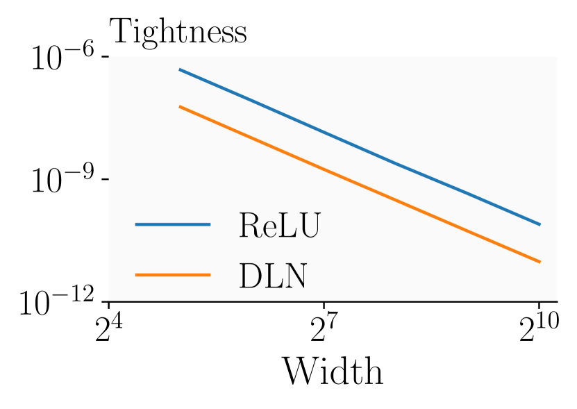
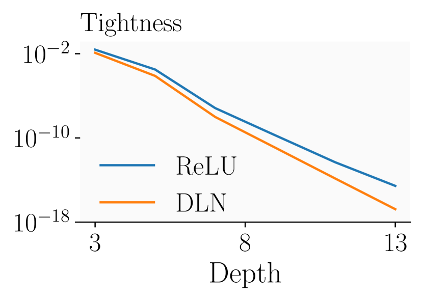
Figure 2: Dependence of tightness at initialization on width (left) and depth (right).

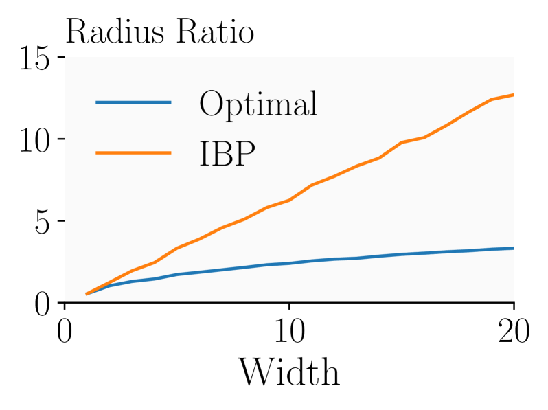
Figure 3: Box reconstruction error on bottleneck width $w$.

4.1 Confirming Interactions of Network Architecture and Tightness

We first confirm the predictiveness of our theoretical results regarding the effect of network width and depth on tightness at initialization and after training for ReLU networks.

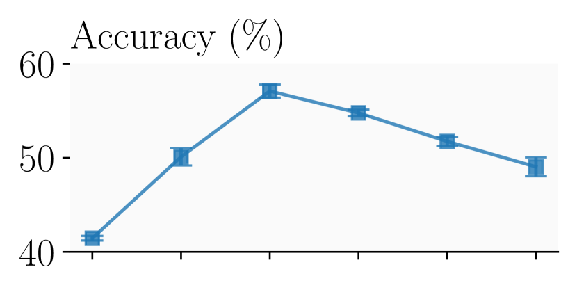
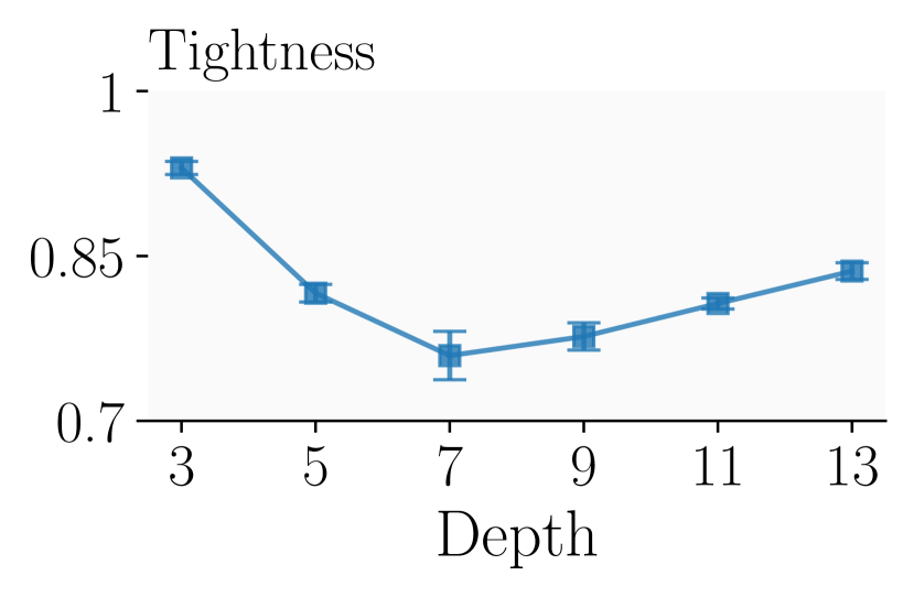
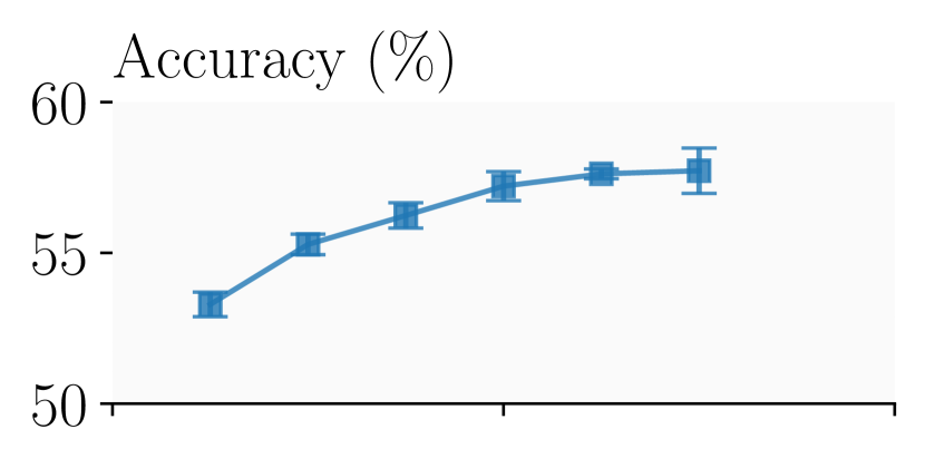
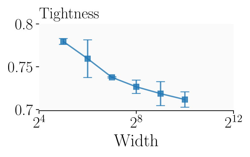
Figure 4: Effect of network depth (top) and width (bottom) on tightness and training set IBP-certified accuracy

In Figure 3 we visualize tightness at initialization, depending on the network width and depth for DLNs and ReLU networks. As predicted by Lemmas 3.7 and 3.8, tightness decreases polynomially with width Figure 3 (left) and exponentially with depth Figure 3 (right) for DLNs. We observe that both of these trends carry over perfectly to ReLU networks. Before turning to networks trained on real datasets, we confirm our predictions on the inherent hardness of linear reconstruction in Figure 3, where we plot the ratio of recovered and original box radius for optimal and IBP propagation, given a bottleneck layer of width $w$ and data with intrinsic dimensionality $k=w$. As predicted by Theorem 3.10, IBP propagation leads to linear growth while optimal propagation yields sublinear growth.

Next, we study the interaction of network architecture and IBP training. To this end, we train networks with 3 to 13 layers on CIFAR-10 for ${\epsilon}=2/255$, visualizing results in Figure 4 (top). To measure the regularizing effect of propagation tightness, we report IBP-certified accuracy on the training set as a measure of the goodness of fit. Generally, we would expect that increasing network depth increases capacity, thus reducing the robust training loss and increasing training set IBP-certified accuracy. However, we only observe such an increase in accuracy until a depth of 7 layers before accuracy starts to drop. We can explain this by analyzing the corresponding tightness. As expected, tightness is high for shallow networks but decreases quickly with depth, reaching a minimum for 7 layers. From there, tightness increases again, at the cost of stronger regularization, explaining the drop in accuracy. This is in line with the popularity of the 7-layer CNN7 in the certified training literature [7, 8, 10].

Continuing our study of architecture effects, we train networks with 0.5 to 16 times the width of a standard CNN7 using IBP training and visualize the resulting IBP certified train set accuracy and tightness in Figure 4 (bottom). We observe that increasing capacity via width instead of depth yields a monotone although diminishing increase in accuracy as tightness decreases gradually. The different trends for width and depth increases agree well with our theoretical results, predicting that sufficient network width is essential for trained networks (see Theorem 3.10). It can further be explained by the observation that increasing depth, at initialization, reduces tightness exponentially, while increasing width only reduces it polynomially. Intuitively, this suggests that less regularization is required to offset the tightness penalty of increasing network width rather than depth networks.

Table 1: Certified and standard Accuracy of SABR-trained models with the original (from Müller et al. [30]) and wider width.

Dataset	$\epsilon$	Width	Accuracy	Certified
MNIST	$0.3$		98.82	93.38
		4x	98.48	93.85
CIFAR-10	$\frac{2}{255}$		79.24	62.84
		2x	79.89	63.28

As these experiments indicate that optimal architectures for IBP-based training methods have only moderate depth but large width, we train wider versions of the popular CNN7 using SABR [10]. Indeed, we observe that this improves upon the state-of-the-art certified accuracy in several settings, shown in Table 1. While these improvements might seem marginal, they are of similar magnitude as multiple years of progress on certified training methods.

4.2 Certified Training Increases Tightness

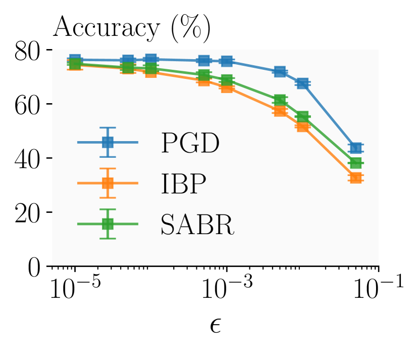
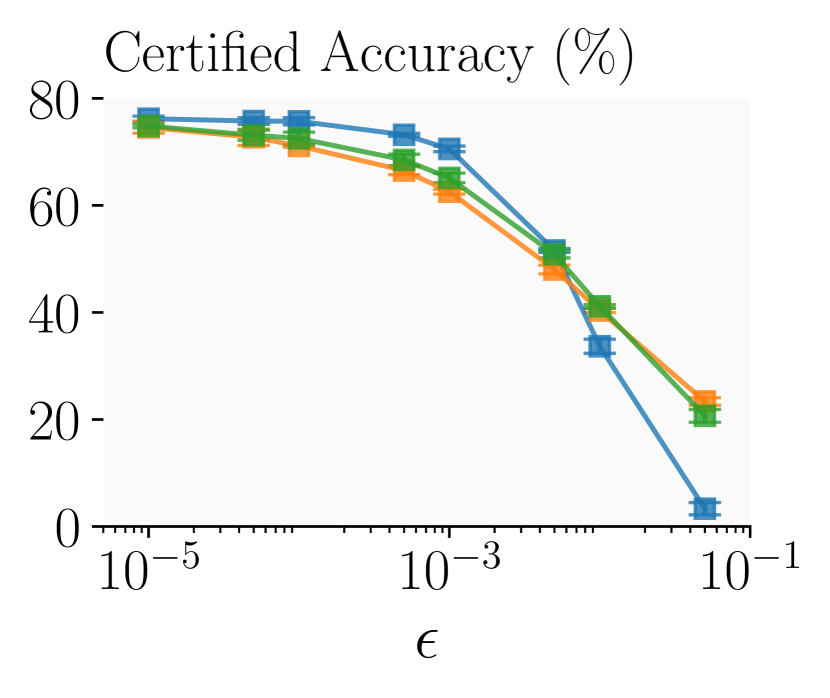
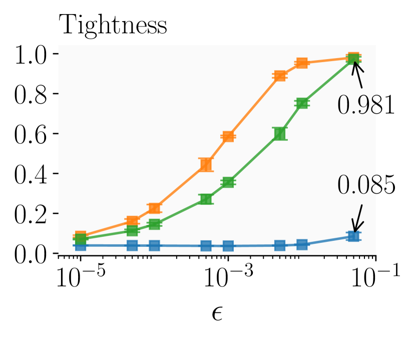
Figure 5: Standard and certified accuracy and tightness for CNN3 on CIFAR-10 depending on training method and perturbation magnitude $\epsilon$ used for training and evaluation.

To assess how different training methods affect tightness, we train a CNN3 on CIFAR-10 for a wide range of perturbation magnitudes ($\epsilon\in[10^{-5},5\cdot 10^{-2}]$) using IBP, PGD, and SABR training, illustrating the resulting tightness and accuracies in Figure 5. Recall, that while IBP computes and optimizes a sound over-approximation of the worst-case loss over the whole input region, SABR propagates only a small adversarially selected subregion with IBP, thus yielding an unsound but generally more precise approximation of the worst-case loss. PGD, in contrast, does not use IBP at all but rather trains with samples that approximately maximize the worst-case loss. We observe that training with either IBP-based method increases tightness with perturbation magnitude until networks become almost propagation invariant for $\epsilon=0.05$ with a tightness of $\tau=0.98$. This confirms our theoretical results, showing that IBP training increases tightness with ${\epsilon}$ (see Theorem 3.9). In contrast, training with PGD barely influences tightness. We observe that the regularization required to yield such high tightness comes at the cost of severely reduced standard accuracies with drops being more pronounced the more a method increases tightness. However, while this reduced standard accuracy translates to smaller certified accuracies for very small perturbation magnitudes (${\epsilon}\leq 5\cdot 10^{-3}$), the increased tightness improves certifiability sufficiently to yield higher certified accuracies for larger perturbation magnitudes (${\epsilon}\geq 10^{-2}$).

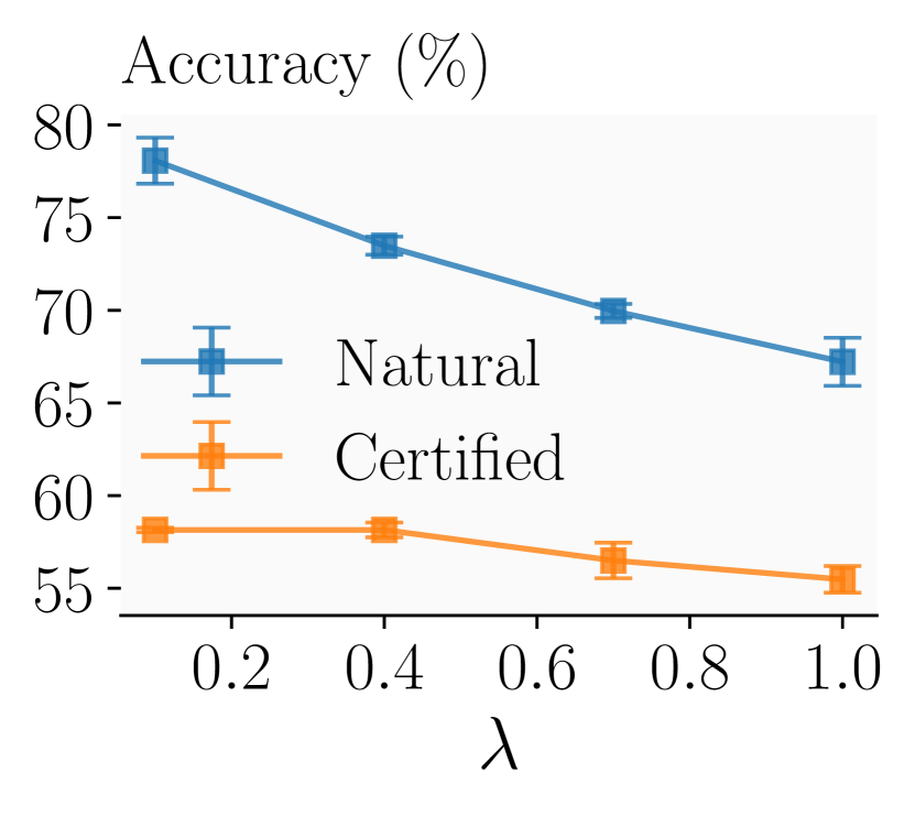
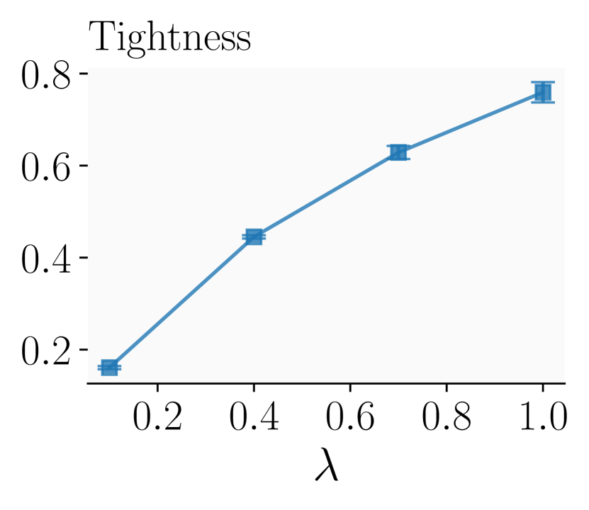
Figure 6: Accuracies and tightness of a CNN7 for CIFAR-10 $\epsilon=\frac{2}{255}$ depending on regularization strength with SABR.

We further investigate this dependency between (certified) robustness and tightness by varying the subselection ratio $\lambda$ when training with SABR. Recall that $\lambda$ controls the size of the propagated regions for a fixed perturbation magnitude ${\epsilon}$, with $\lambda=1$ recovering IBP and $\lambda=0$ PGD. Plotting results in Figure 6, we observe that while decreasing lambda severely reduces tightness and thus regularization it not only leads to increasing natural but also certified accuracies until tightness falls below $\tau<0.5$ at $\lambda=0.4$. This again highlights that reducing tightness while maintaining sufficient certifiability is a promising path to new certified training methods. We observe similar trends when varying the regularization level for other unsound certified training methods, discussed in Section D.1.

Table 2: Comparison of IBP- and non-IBP-based training methods.

Method	${\epsilon}$	Accuracy	Tightness	Certified
PGD	2/255	81.2	0.001	-
	8/255	69.3	0.007	-
COLT	2/255	78.4	0.009	60.7
	8/255	51.7	0.057	26.7
SABR	2/255	75.6	0.182	57.7
	8/255	48.2	0.950	31.2
IBP	2/255	63.0	0.803	51.3
	8/255	42.2	0.977	31.0

We now investigate whether non-IBP-based certified training methods affect a similar increase in tightness as IBP-based methods. To this end, we consider COLT [18] which combines precise Zonotope bounds with adversarial training. However, as COLT does not scale to the popular CNN7, we compare with it on the 4-layer CNN architecture used by Balunovic and Vechev [18]. Comparing tightness and certified and standard accuracies in Table 2, we observe that the ordering of tightness and accuracy is exactly inverted, thus highlighting the large accuracy penalty associated with the strong regularization for tightness. While COLT only affects a minimal increase in tightness compared to SABR or IBP, it still yields networks, an order of magnitude tighter than PGD, suggesting that slightly increased tightness might be desirable for certified robustness. This is further corroborated by the observation that while COLT reaches the highest certified accuracies at small perturbation magnitudes, the more heavily regularizing SABR performs better at larger perturbation magnitudes.

5 Related Work

Certified Training

Sound certified training methods compute and optimize an over-approximation of the worst-case loss obtained via bound propagation methods [34, 19, 17]. A particularly efficient and scalable method is IBP [7, 14], for which Shi et al. [8] propose a custom initialization scheme, significantly shortening training schedules, and Lin et al. [24] propose a non-negativity regularization, marginally improving certified accuracies. More recent methods use unsound but more precise approximations. COLT [18] combines precise Zonotope [5] bounds with adversarial training but is severely limited in scalability. IBP-R [12] combines an IBP-based regularization with adversarial training at larger perturbation magnitudes. SABR [10] applies IBP to small but carefully selected regions in the adversary specification to reduce regularization. TAPS [11], similar to COLT, combines IBP with adversarial training. This recent dominance of IBP-based methods motivates our work to develop a deeper understanding of how IBP training affects network robustness.

Theoretical Analysis of IBP

The capability of IBP has been studied theoretically in the past. Baader et al. [35] first show that continuous functions can be approximated by IBP-certifiable ReLU networks up to arbitrary precision. Wang et al. [36] extend this result to more activation functions and prove that constructing such networks is strictly harder than NP-complete problems assuming coNP $\notin$ NP. Wang et al. [37] study the convergence of IBP-training and find that it converges to a global optimum with high probability for infinite width. Mirman et al. [38] derive a negative result, showing that even optimal box bounds can fail on simple datasets. However, none of these works study the tightness of IBP bounds, , their relationship to optimal interval approximations. Motivated by recent certified training methods identifying this approximation precision as crucial [30, 11], we bridge this gap by deriving sufficient and necessary conditions for propagation invariance, introducing the relaxed measure of propagation tightness and studying how it interacts with network architecture and IBP training, both theoretically and empirically.

6 Conclusion

Motivated by the recent and surprising dominance of IBP-based certified training methods, we investigated its underlying mechanisms and trade-offs. By quantifying the relationship between IBP and optimal Box bounds with our novel propagation tightness metric we were able to predict the influence of architecture choices on deep linear networks at initialization and after training. Our experimental results confirm the applicability of these theoretical results to deep ReLU networks and show that wider networks improve the performance of state-of-the-art methods, while deeper networks do not. Finally, we show that IBP-based certified training methods, in contrast to non-IBP-based methods, significantly increase propagation tightness at the cost of strong regularization. We believe that this insight and the novel metric of propagation tightness will constitute a key step towards developing novel and more effective certified training methods.

Appendix A Additional Theoretical Results

Below we present a corollary, formalizing the intutions we provided in Section 3.2.

Corollary A.1.

Assume all elements of ${\bm{W}}^{(1)}$, ${\bm{W}}^{(2)}$ and ${\bm{W}}^{(2)}{\bm{W}}^{(1)}$ are non-zero and ${\bm{W}}^{(2)}{\bm{W}}^{(1)}$ is propagation invariant. Then choosing the signs of one row and one column of ${\bm{W}}^{(2)}{\bm{W}}^{(1)}$ fixes all signs of ${\bm{W}}^{(2)}{\bm{W}}^{(1)}$.

Proof.

For notational reasons, we define $W:=W^{(2)}W^{(1)}$. Without loss of generality, assume we know the signs of the first row and the first column, , $W_{1,\cdot}$ and $W_{\cdot,1}$. We prove via a construction of the signs of all elements. The construction is given by the following: whenever $\exists i,j$, such that we know the sign of $W_{i,j}$, $W_{i,j+1}$ and $W_{i+1,j}$, we fix the sign of $W_{i+1,j+1}$ to be positive if there are an odd number of positive elements among $W_{i,j}$, $W_{i,j+1}$ and $W_{i+1,j}$, otherwise negative.

By Theorem 3.4, propagation invariance requires us to fix the sign of the last element in the $W_{i:i+1,j:j+1}$ block in this way. We only need to prove that when this process terminates, we fix the signs of all elements. We show this via recursion.

When $i=1$ and $j=1$, we have known the signs of $W_{i,j}$, $W_{i,j+1}$ and $W_{i+1,j}$, thus the sign of $W_{i+1,j+1}$ is fixed. Continuing towards the right, we gradually fix the sign of $W_{2,j+1}$ for $j=1,\dots,d-1$. Continuing downwards, we gradually fix the sign of $W_{i+1,2}$ for $i=1,\dots,d-1$. Therefore, all signs of the elements of the second row and the second column are fixed. By recursion, we would finally fix all the rows and the columns, thus the whole matrix. ∎

Appendix B Deferred Proofs

Proof of Lemma 3.1

Here we prove Lemma 3.1, restated below for convenience.

See 3.1

Proof.

On the one hand, assume $y_{i}-y_{\text{true}}<0$ for all $i$. Then for the $i^{th}$ output dimension, the optimal bounding box is $\max y_{i}-y_{\text{true}}$. Since the classifier is continuous, ${\bm{f}}(\mathcal{B}({\bm{x}},\bm{\epsilon}))$ is a closed and bounded set. Therefore, by extreme value theorem, $\exists\eta\in\mathcal{B}({\bm{x}},\bm{\epsilon})$ such that $\eta=\operatorname*{arg\,max}y_{i}-y_{\text{true}}$, thus $\max y_{i}-y_{\text{true}}<0$. Since this holds for every $i$, $\operatorname*{Box}^{*}({\bm{f}},\mathcal{B}({\bm{x}},\bm{\epsilon}))\subseteq\mathcal{R}_{<0}^{K-1}$.

On the other hand, assume $\operatorname*{Box}^{*}({\bm{f}},\mathcal{B}({\bm{x}},\bm{\epsilon}))\subseteq\mathcal{R}_{<0}^{K-1}$. Since ${\bm{f}}(\mathcal{B}({\bm{x}},\bm{\epsilon}))\subseteq\operatorname*{Box}^{*}({\bm{f}},\mathcal{B}({\bm{x}},\bm{\epsilon}))\subseteq\mathcal{R}_{<0}^{K-1}$, we get $y_{i}-y_{\text{true}}<0$ for all $i$. ∎

Proof of Theorem 3.2

We first prove Theorem 3.2 for a 2-layer DLN as Lemma B.1.

Lemma B.1.

For a two-layer DLN ${\bm{f}}={\bm{W}}^{(2)}{\bm{W}}^{(1)}$, $(\overline{{\bm{z}}}^{*}-\underline{{\bm{z}}}^{*})/2=\left|W^{(2)}W^{(1)}\right|\bm{\epsilon}$ and $(\overline{{\bm{z}}}^{\dagger}-\underline{{\bm{z}}}^{\dagger})/2=\left|W^{(2)}\right|\left|W^{(1)}\right|\bm{\epsilon}$. In addition, $\operatorname*{Box}^{*}$ and $\operatorname*{Box}^{\dagger}$ have the same center ${\bm{f}}({\bm{x}})$.

Proof.

First, assume $W^{(1)}\in\mathcal{R}^{d_{1}\times d_{0}}$, $W^{(2)}\in\mathcal{R}^{d_{2}\times d_{1}}$ and $B_{i}=[-1,1]^{d_{i}}$ for $i=0,1,2$, where $d_{i}\in\mathcal{Z}_{+}$ are some positive integers. The input box can be represented as $\operatorname*{diag}(\epsilon_{0})B_{0}+b$ for $\epsilon_{0}=\epsilon$.

For a single linear layer, the box propagation yields

$$\operatorname*{Box}(W^{(1)}(\operatorname*{diag}(\epsilon_{0})B_{0}+b))$$

$$=\operatorname*{Box}(W^{(1)}\operatorname*{diag}(\epsilon_{0})B_{0})+W^{(1)}b$$

$$=\operatorname*{diag}\left(\sum_{j=1}^{d_{0}}|W^{(1)}_{i,j}|\epsilon_{0}[j]\right)B_{1}+W^{(1)}b$$

$$:=\operatorname*{diag}(\epsilon_{1})B_{1}+W^{(1)}b.$$ (5)

Applying Equation 5 iteratively, we get the explicit formula of layer-wise propagation for two-layer linear network:

$$\operatorname*{Box}(W^{(2)}\operatorname*{Box}(W^{(1)}(\operatorname*{diag}(\epsilon_{0})B_{0}+b)))$$

$$=\operatorname*{Box}\left(W^{(2)}(\operatorname*{diag}(\epsilon_{1})B_{1}+W^{(1)}b)\right)$$

$$=\operatorname*{diag}\left(\sum_{k=1}^{d_{1}}|W^{(2)}_{i,k}|\epsilon_{1}[k]\right)B_{2}+W^{(2)}W^{(1)}b$$

$$=\operatorname*{diag}\left(\sum_{j=1}^{d_{0}}\epsilon_{0}[j]\left(\sum_{k=1}^{d_{1}}|W^{(2)}_{i,k}W^{(1)}_{k,j}|\right)\right)B_{2}$$

$$\quad+W^{(2)}W^{(1)}b.$$ (6)

Applying Equation 5 on $W:=W^{(2)}W^{(1)}$, we get the explicit formula of the tightest box:

$$\operatorname*{Box}(W^{(2)}W^{(1)}(\operatorname*{diag}(\epsilon_{0})B_{0}+b))$$

$$=\operatorname*{diag}\left(\sum_{j=1}^{d_{0}}|(W^{(2)}W^{(1)})_{i,j}|\epsilon_{0}[j]\right)B_{2}+W^{(2)}W^{(1)}b$$

$$=\operatorname*{diag}\left(\sum_{j=1}^{d_{0}}\epsilon_{0}[j]\left|\sum_{k=1}^{d_{1}}W^{(2)}_{i,k}W^{(1)}_{k,j}\right|\right)B_{2}$$

$$\quad+W^{(2)}W^{(1)}b.$$ (7)

∎

Now, we use induction and Lemma B.1 to prove Theorem 3.2, restated below for convenience. The key insight is that a multi-layer DLN is equivalent to a single-layer linear network. Thus, we can group layers together and view general DLNs as two-layer DLNs.

See 3.2

Proof.

For $L=2$, by Lemma B.1, the result holds. Assume for $L\leq m$, the result holds. Therefore, for $L=m+1$, we group the first $m$ layers as a single layer, resulting in a “two” layer equivalent network. Thus, $(\overline{{\bm{z}}}^{*}-\underline{{\bm{z}}}^{*})/2=\left|{\bm{W}}^{(m+1)}\Pi_{k=1}^{m}{\bm{W}}^{(k)}\right|\bm{\epsilon}=\left|\Pi_{k=1}^{L}{\bm{W}}^{(k)}\right|\bm{\epsilon}$. Similarly, by Equation 5, we can prove $(\overline{{\bm{z}}}^{*}-\underline{{\bm{z}}}^{*})/2=\left(\left|{\bm{W}}^{(m+1)}\right|\Pi_{k=1}^{m}\left|{\bm{W}}^{(k)}\right|\right)\bm{\epsilon}=\left(\Pi_{k=1}^{L}\left|{\bm{W}}^{(k)}\right|\right)\bm{\epsilon}$. The claim about center follows by induction similarly. ∎

Proof of Lemma 3.3

Here, we prove Lemma 3.3, restated below for convenience.

See 3.3

Proof.

We prove the statement via comparing the box bounds. By Lemma B.1, we need $\left|\sum_{k=1}^{d_{1}}W^{(2)}_{i,k}W^{(1)}_{k,j}\right|=\sum_{k=1}^{d_{1}}|W^{(2)}_{i,k}W^{(1)}_{k,j}|$. The triangle inequality of absolute function says this holds if and only if $W^{(2)}_{i,k}W^{(1)}_{k,j}\geq 0$ for all $k$ or $W^{(2)}_{i,k}W^{(1)}_{k,j}\leq 0$ for all $k$. ∎

Proof of Theorem 3.4

Here, we prove Theorem 3.4, restated below for convenience.

See 3.4

Proof.

The assumption $(W^{(2)}W^{(1)})_{i,j}\cdot(W^{(2)}W^{(1)})_{i,j^{\prime}}\cdot(W^{(2)}W^{(1)})_{i^{\prime},j}\cdot(W^{(2)}W^{(1)})_{i^{\prime},j^{\prime}}<0$ implies three elements are of the same sign while the other element has a different sign. Without loss of generality, assume $(W^{(2)}W^{(1)})_{i^{\prime},j^{\prime}}<0$ and the rest three are all positive.

Assume $W^{(2)}W^{(1)}$ is propagation invariant. By Lemma 3.3, this means $W^{(2)}_{i,\cdot}.\text{sign}=W^{(1)}_{\cdot,j}.\text{sign}$, $W^{(2)}_{i,\cdot}.\text{sign}=W^{(1)}_{\cdot,j^{\prime}}.\text{sign}$, $W^{(2)}_{i^{\prime},\cdot}.\text{sign}=W^{(1)}_{\cdot,j}.\text{sign}$ and $W^{(2)}_{i^{\prime},\cdot}.\text{sign}=-W^{(1)}_{\cdot,j^{\prime}}.\text{sign}$. Therefore, we have $-W^{(1)}_{\cdot,j^{\prime}}.\text{sign}=W^{(1)}_{\cdot,j^{\prime}}.\text{sign}$, which implies all elements of $W^{(1)}_{\cdot,j^{\prime}}$ must be zero. However, this results in $(W^{(2)}W^{(1)})_{i,j^{\prime}}=0$, a contradiction. ∎

Proof of Lemma 3.7

Here, we prove Lemma 3.7, restated below for convenience.

See 3.7

Proof.

We first compute the size of the layer-wisely propagated box. From Equation 6, we get that for the $i$-th dimension,

$$\mathbb{E}(u_{i}-l_{i}) =\mathbb{E}\left(\sum_{j=1}^{d_{0}}\epsilon_{0}[j]\left(\sum_{k=1}^{d_{1}}|W^{(2)}_{i,k}W^{(1)}_{k,j}|\right)\right)$$

$$=\sum_{j=1}^{d_{0}}\epsilon_{0}[j]\left(\sum_{k=1}^{d_{1}}\mathbb{E}(|W^{(2)}_{i,k}|)\cdot\mathbb{E}(|W^{(1)}_{k,j}|)\right)$$

$$=\sigma_{1}\sigma_{2}\sum_{j=1}^{d_{0}}\epsilon_{0}[j]\left(\sum_{k=1}^{d_{1}}\mathbb{E}(|\mathcal{N}(0,1)|)^{2})\right).$$

Since $\mathbb{E}(|\mathcal{N}(0,1)|)=\sqrt{\frac{2}{\pi}}$ , we have

$$\mathbb{E}(u_{i}-l_{i})=\frac{2}{\pi}\sigma_{1}\sigma_{2}d_{1}\|\epsilon_{0}\|_{1}.$$ (8)

Now we compute the size of the tightest box. From Equation 7, we get that for the $i$-th dimension,

$$\mathbb{E}(u_{i}^{*}-l_{i}^{*}) =\mathbb{E}\left(\sum_{j=1}^{d_{0}}\epsilon_{0}[j]\left|\sum_{k=1}^{d_{1}}W^{(2)}_{i,k}W^{(1)}_{k,j}\right|\right)$$

$$=\sigma_{1}\sigma_{2}\sum_{j=1}^{d_{0}}\epsilon_{0}[j]\mathbb{E}\left(\left|\sum_{k=1}^{d_{1}}X_{k}Y_{k}\right|\right),$$

where $X_{k}$ and $Y_{k}$ are i.i.d. standard Gaussian random variables. Using the law of total expectation, we have

$$\mathbb{E}\left(\left|\sum_{k=1}^{d_{1}}X_{k}Y_{k}\right|\right) =\mathbb{E}\left(\mathbb{E}\left(\left|\sum_{k=1}^{d_{1}}X_{k}Y_{k}\right|\;\middle|\;Y_{k}\right)\right)$$

$$=\mathbb{E}\left(\mathbb{E}\left(\left|\mathcal{N}(0,\sum_{k=1}^{d_{1}}Y_{k}^{2})\right|\;\middle|\;Y_{k}\right)\right)$$

$$=\sqrt{\frac{2}{\pi}}\mathbb{E}\left(\sqrt{\sum_{k=1}^{d_{1}}Y_{k}^{2}}\right)$$

$$=\sqrt{\frac{2}{\pi}}\mathbb{E}(\sqrt{\chi^{2}(d_{1})}).$$

Since $\mathbb{E}(\sqrt{\chi^{2}(d_{1})})=\sqrt{2}\Gamma(\frac{1}{2}(d_{1}+1))/\Gamma(\frac{1}{2}d_{1})$, we have

$$\mathbb{E}(u_{i}^{*}-l_{i}^{*})=\frac{2}{\sqrt{\pi}}\sigma_{1}\sigma_{2}\|\epsilon_{0}\|_{1}\Gamma(\frac{1}{2}(d_{1}+1))/\Gamma(\frac{1}{2}d_{1}).$$ (9)

Combining Equation 8 and Equation 9, we have:

$$\frac{\mathbb{E}(u_{i}-l_{i})}{\mathbb{E}(u_{i}^{*}-l_{i}^{*})}=\frac{d_{1}\Gamma(\frac{1}{2}d_{1})}{\sqrt{\pi}\Gamma(\frac{1}{2}(d_{1}+1))}.$$ (10)

To see the asymptotic behavior, use $\Gamma(x+\alpha)/\Gamma(x)\sim x^{\alpha}$, we have

$$\frac{\mathbb{E}(u_{i}-l_{i})}{\mathbb{E}(u_{i}^{*}-l_{i}^{*})}\sim\frac{1}{\sqrt{\pi}}d_{1}^{\frac{1}{2}}.$$ (11)

To establish the bounds on the minimum expected slackness, we use Lemma B.2. ∎

Lemma B.2.

Let $g(n):=\frac{n\Gamma(\frac{1}{2}n)}{\sqrt{\pi}\Gamma(\frac{1}{2}(n+1))}$. $g(n)$ is monotonically increasing for $n\geq 1$. Thus, for $n\geq 2$, $g(n)\geq g(2)>1.27$.

Proof.

Using polygamma function $\psi^{(0)}(z)=\Gamma^{\prime}(z)/\Gamma(z)$, we have

$$g^{\prime}(n)\propto 1+\frac{1}{2}n\left(\psi^{(0)}\left(\frac{1}{2}n\right)-\psi^{(0)}\left(\frac{1}{2}(n+1)\right)\right).$$

Using the fact that $\psi^{(0)}(z)$ is monotonically increasing for $z>0$ and $\psi^{(0)}(z+1)=\psi^{(0)}(z)+\frac{1}{z}$, we have

$$1+\frac{1}{2}n\left(\psi^{(0)}\left(\frac{1}{2}n\right)-\psi^{(0)}\left(\frac{1}{2}(n+1)\right)\right)$$

$$>1+\frac{1}{2}n\left(\psi^{(0)}\left(\frac{1}{2}n\right)-\psi^{(0)}\left(\frac{1}{2}n+1\right)\right)$$

$$=1+\frac{1}{2}n\left(-\frac{2}{n}\right)$$

$$=0.$$

Therefore, $g^{\prime}(n)$ is strictly positive for $n\geq 1$, and thus $g(n)$ is monotonically increasing for $n\geq 1$. ∎

As a final comment, we visualize $g(n)$ in Figure 7. As expected, $g(n)$ is monotonically increasing in the order of $O(\sqrt{n})$.

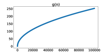
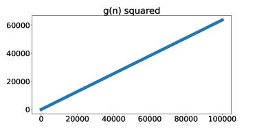
Figure 7: $g(n)$ and $g^{2}(n)$ visualized.

Proof of Corollary 3.8

Here, we prove Corollary 3.8, restated below for convenience.

See 3.8

Proof.

This is pretty straightforward and only requires a coarse application of Lemma 3.7. Without loss of generality, we assume $L$ is even. If $L$ is odd, then we simply discard the slackness introduced by the last layer, , assume the last layer does not introduce additional slackness.

We group the $2i-1$-th and $2i$-th layer as a new layer. By Lemma 3.7, these $L/2$ subnetworks all introduce an additional slackness factor of $\tau$. Note that Equation 8 implies that the size of the output box is proportional to the size of the input box. Therefore, the layer-wisely propagated box of $\Pi_{i=1}^{L}W_{i}$ is $\tau^{L/2}$ looser than the layer-wisely propagated box of $\Pi_{j=1}^{L/2}(W_{2j-1}W_{2j})$. In addition, the size of the tightest box for $\Pi_{i=1}^{L}W_{i}$ is upper bounded by layer-wisely propagating $\Pi_{j=1}^{L/2}(W_{2j-1}W_{2j})$. Therefore, the minimum expected slackness is lower bounded by $\tau^{L/2}$. ∎

Proof of Theorem 3.9

Here, we prove Theorem 3.9, restated below for convenience.

See 3.9

Proof.

We prove a stronger claim: $\langle\nabla_{\theta}(R(\bm{\epsilon}+\Delta\bm{\epsilon})-R(\bm{\epsilon})),\nabla_{\theta}\tau\rangle\leq 0$ for all $\bm{\epsilon}\geq 0$ and $\Delta\bm{\epsilon}>0$. Let $\bm{\epsilon}=\bm{0}$ yields the theorem.

We prove the claim for $\Delta\bm{\epsilon}\rightarrow 0$. For large $\Delta\bm{\epsilon}$, we can break it into $R(\bm{\epsilon}+\Delta\bm{\epsilon})-R(\bm{\epsilon})=\sum_{i=1}^{n}R(\bm{\epsilon}+\frac{i}{n}\Delta\bm{\epsilon})-R(\bm{\epsilon}+\frac{i-1}{n}\Delta\bm{\epsilon})$, thus proving the claim since each summand satisfies the theorem.

Let $L_{1}=R(\bm{\epsilon})$ and $L_{2}=R(\bm{\epsilon}+\Delta\bm{\epsilon})$. By Taylor expansion, we have $L_{2}=L_{1}+\Delta\bm{\epsilon}^{\top}{\bm{W}}^{\dagger}\nabla_{\bm{u}}g=L_{1}+\frac{1}{\tau}\Delta\bm{\epsilon}^{\top}{\bm{W}}^{*}\nabla_{\bm{u}}g$, where $\nabla_{\bm{u}}g=\nabla_{\bm{u}}g({\bm{u}})$ evaluated at ${\bm{u}}={\bm{W}}^{\dagger}\bm{\epsilon}$. Note that the increase of $\bm{\epsilon}$ would increase the risk, thus $\nabla_{\bm{u}}g\geq\bm{0}$.

For the $i^{\text{th}}$ parameter $\theta_{i}$, $\nabla_{\theta_{i}}(L_{2}-L_{1})\nabla_{\theta_{i}}\tau=\frac{1}{\tau^{2}}\Delta\bm{\epsilon}^{\top}(\tau\nabla_{\theta_{i}}{\bm{W}}^{*}-{\bm{W}}^{*}\nabla_{\theta_{i}}\tau)\nabla_{\bm{u}}g\nabla_{\theta_{i}}\tau$. Thus, $\langle\nabla_{\theta}(L_{2}-L_{1}),\nabla_{\theta}\tau\rangle=\frac{1}{\tau^{2}}\Delta\bm{\epsilon}^{\top}(\tau\sum_{i}\nabla_{\theta_{i}}\tau\cdot\nabla_{\theta_{i}}{\bm{W}}^{*}-{\bm{W}}^{*}\|\nabla_{\theta}\tau\|_{2}^{2})\nabla_{{\bm{u}}}g$. Since $\Delta\bm{\epsilon}>\bm{0}$ and $\nabla_{\bm{u}}g\geq\bm{0}$, it sufficies to prove that $\tau\sum_{i}\nabla_{\theta_{i}}\tau\cdot\nabla_{\theta_{i}}{\bm{W}}^{*}-{\bm{W}}^{*}\|\nabla_{\theta}\tau\|_{2}^{2}$ is nonpositive, , $\tau\langle\nabla_{\theta}\tau,\nabla_{\theta}{\bm{W}}^{*}_{ij}\rangle-{\bm{W}}^{*}_{ij}\|\nabla_{\theta}\tau\|_{2}^{2}$ is nonpositive for every $i,j$.

Since $\|{\bm{u}}\|_{2}\|{\bm{v}}\|_{2}\geq\langle{\bm{u}},{\bm{v}}\rangle$, we have

$$\quad\quad\frac{\|\nabla_{\theta}{\bm{W}}^{*}_{ij}\|_{2}}{{\bm{W}}^{*}_{ij}}\leq\frac{1}{2}\frac{\|\nabla_{\theta}{\bm{W}}^{\dagger}_{ij}\|_{2}}{{\bm{W}}^{\dagger}_{ij}}$$

$$\Rightarrow\|\nabla_{\theta}\log{\bm{W}}^{\dagger}\|_{2}\geq 2\|\nabla_{\theta}\log{\bm{W}}^{*}\|_{2}$$

$$\Rightarrow\|\nabla_{\theta}\log{\bm{W}}^{\dagger}\|_{2}^{2}\geq 2\langle\nabla_{\theta}\log{\bm{W}}^{\dagger},\nabla_{\theta}\log{\bm{W}}^{*}\rangle$$

Therfore, $\|\nabla_{\theta}\log\tau\|_{2}^{2}=\|\nabla_{\theta}(\log{\bm{W}}^{*}_{ij}-\log{\bm{W}}^{\dagger}_{ij})\|_{2}^{2}=\|\nabla_{\theta}\log{\bm{W}}^{*}_{ij}\|_{2}^{2}-2\langle\nabla_{\theta}\log{\bm{W}}^{\dagger},\nabla_{\theta}\log{\bm{W}}^{*}\rangle+\|\nabla_{\theta}\log{\bm{W}}^{\dagger}\|_{2}^{2}\geq\|\nabla_{\theta}\log{\bm{W}}^{*}_{ij}\|_{2}^{2}$. This means $\frac{\|\nabla_{\theta}{\bm{W}}^{*}_{ij}\|_{2}}{{\bm{W}}^{*}_{ij}}\leq\frac{\|\nabla_{\theta}\tau\|_{2}}{\tau}$, thus ${\bm{W}}^{*}_{ij}\|\nabla_{\theta}\tau\|_{2}^{2}\geq\tau\|\nabla_{\theta}\tau\|_{2}\|\nabla_{\theta}{\bm{W}}^{*}_{ij}\|_{2}\geq\tau\langle\nabla_{\theta}\tau,\nabla_{\theta}{\bm{W}}^{*}_{ij}\rangle$, which fulfills our goal. ∎

Proof of Theorem 3.10

Here, we prove Theorem 3.10, restated below for convenience.

See 3.10

Proof.

Since box propagation for linear functions maps the center of the input box to the center of the output box, the center of the output box is exactly $\hat{X}$. By Lemma B.1, we have $\bm{\delta}=|U_{k}||U_{k}|^{\top}\epsilon\bm{1}$. For notational simplicity, let $V=|U_{k}|$, thus

$$\bm{\delta}_{i} =\sum_{j=1}^{k}V_{ij}(\sum_{p=1}^{d}V^{\top}_{jp}\epsilon)$$

$$=\epsilon\sum_{p=1}^{d}\sum_{j=1}^{k}V_{ij}V_{pj}$$

$$=\epsilon\sum_{j=1}^{k}V_{ij}\|V_{:j}\|_{1}.$$

Therefore, $\mathbb{E}\bm{\delta}_{i}/\epsilon=\sum_{j=1}^{k}\mathbb{E}(V_{ij}\|V_{:j}\|_{1})=ck$, where $c=\mathbb{E}(V_{ij}\|V_{:j}\|_{1})$. Since $V_{:j}$ is the absolute value of a column of the orthogonal matrix uniformly drawn, $V_{:j}$ itself is the absolute value of a vector drawn uniformly from the unit hyper-ball. By Cook [39] and Marsaglia [40], $V_{:j}$ is equivalent in distribution to i.i.d. draw samples from the standard Gaussian for each dimension and then normalize it by its $L_{2}$ norm. For notational simplicity, let $V_{:j}\overset{d}{=}v=|u|$, where $u=\hat{u}/\|\hat{u}\|_{2}$ and all dimensions of $\hat{u}$ are i.i.d. drawn from the standard Gaussian distribution, thus $c=\mathbb{E}(v_{1}\|v\|_{1})$.

Expanding $\|v\|_{1}$, we have $c=\mathbb{E}(v_{1}^{2})+\sum_{i=2}^{d}\mathbb{E}(v_{1}v_{i})=\frac{1}{d}\mathbb{E}(\|v\|_{2}^{2})+(d-1)\mathbb{E}(v_{1}v_{2})=\frac{1}{d}+(d-1)\mathbb{E}(v_{1}v_{2})$. From page 20 of Pinelis and Molzon [41], we know each entry in $u$ converges to $\mathcal{N}(0,1/d)$ at $O(1/d)$ speed in Kolmogorov distance. In addition, $\mathbb{E}(v_{1}v_{2})=\mathbb{E}(\mathbb{E}(v_{2}\mid v_{1})\cdot v_{1})=\mathbb{E}(v_{1}\sqrt{1-v_{1}^{2}})\mathbb{E}(v^{\prime}_{2})$, where $v^{\prime}$ is the absolute value of a random vector uniformly drawn from the $d-1$ dimensional sphere. Therefore, for large $d$, $c=(d-1)\mathbb{E}(v_{1}\sqrt{1-v_{1}^{2}})\mathbb{E}(v_{2}^{\prime})=(d-1)\mathbb{E}(v_{1})\mathbb{E}(v_{2}^{\prime})=(d-1)\mathbb{E}(|\mathcal{N}(0,1/d)|)\mathbb{E}(|\mathcal{N}(0,1/(d-1))|)=\frac{2}{\pi}$.

To show how good the asymptotic result is, we run Monte-Carlo to get the estimation of $c$. As shown in the left of Figure 8, the Monte-Carlo result is consistent to this theorem. In addition, it converges very quickly, , stablizing at 0.64 when $d\geq 100$.

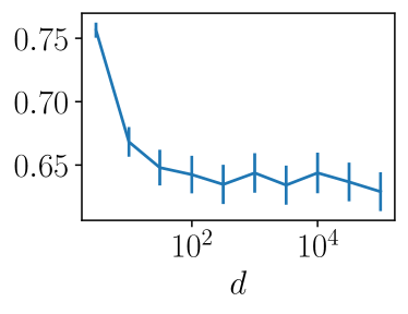
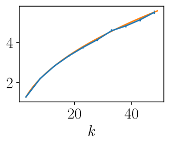
Figure 8: Monte-Carlo estimations of Theorem 3.10. Result bases on 10000 samples for each $d$. Left: $c$ plotted against $d$ in log scale. Right: $\mathbb{E}(\bm{\delta}^{*}_{i})$ plotted against $k$ for $d=2000$ (blue), together with the theoretical predictions (orange).

Now we start proving (2). By Lemma B.1, we have $\delta^{*}=|U_{k}U_{k}^{\top}|\epsilon\bm{1}$. Thus,

$$\mathbb{E}(\bm{\delta}^{*}_{i}/\epsilon) =\sum_{j=1}^{d}\mathbb{E}\left|\sum_{p=1}^{k}U_{ip}U_{jp}\right|$$

$$=\sum_{j\neq i}\mathbb{E}\left|\sum_{p=1}^{k}U_{ip}U_{jp}\right|+\mathbb{E}(\sum_{p=1}^{k}U_{ip}^{2})$$

$$=(d-1)\mathbb{E}\left|\sum_{p=1}^{k}U_{ip}U_{jp}\right|+\frac{k}{d}.$$

In addition, we have

$$\quad(d-1)\mathbb{E}\left|\sum_{p=1}^{k}U_{ip}U_{jp}\right|$$

$$=(d-1)\mathbb{E}_{U_{i}}\left(\mathbb{E}_{U_{j}}\left(\left|\sum_{p=1}^{k}U_{ip}U_{jp}\right|\bigg{|}U_{i}\right)\right)$$

$$\rightarrow(d-1)\mathbb{E}_{U_{i}}\left(\mathbb{E}\left|\mathcal{N}\left(0,\frac{\sum_{p=1}^{k}U_{ip}^{2}}{d-1}\right)\right|\right)$$

$$=(d-1)\sqrt{\frac{2}{\pi(d-1)}}\mathbb{E}\sqrt{\sum_{p=1}^{k}U_{ip}^{2}}$$

$$=\sqrt{\frac{2(d-1)}{\pi}}\mathbb{E}\sqrt{\frac{1}{d}\chi^{2}(k)}$$

$$\rightarrow\frac{2}{\sqrt{\pi}}\frac{\Gamma(\frac{1}{2}(k+1))}{\Gamma(\frac{1}{2}k)},$$

where we use again that for large $d$, the entries of a column tends to Gaussian. This proves (2). The expected tightness follows by definition, , dividing the result of (1) and (2). ∎

The right of Figure 8 plots the Monte-Carlo estimations against our theoretical results. Clearly, this confirms our result.

Appendix C Experimental Details

C.1 Dataset

We use the MNIST [42] and CIFAR-10 [43] datasets for our experiments. Both are open-source and freely available. For MNIST, we do not apply any preprocessing or data augmentation. For CIFAR-10, we normalize images with their mean and standard deviation and, during training, first apply 2-pixel zero padding and then random cropping to $32\times 32$.

C.2 Model Architecture

We follow previous works [8, 10, 11] and use a 7-layer convolutional network CNN7 in most experiments. We also use a simplified 3-layer convolutional network CNN3 in Section 4.2. Details about them can be found in the released code.

C.3 Training

Following previous works [10, 11], we use the initialization, warm-up regularization, and learning schedules introduced by Shi et al. [8]. Specifically, for MNIST, the first 20 epochs are used for $\epsilon$-scheduling, increasing $\epsilon$ smoothly from 0 to the target value. Then, we train an additional 50 epochs with two learning rate decays of 0.2 at epochs 50 and 60, respectively. For CIFAR-10, we use 80 epochs for $\epsilon$-annealing, after training models with standard training for 1 epoch. We continue training for 80 further epochs with two learning rate decays of 0.2 at epochs 120 and 140, respectively. The initial learning rate is $5\times 10^{-3}$ and the gradients are clipped to an $L_{2}$ norm of at most $10.0$ before every step.

C.4 Certification

We apply MN-BaB [4] to certify all models. MN-BaB is a state-of-the-art complete certification method built on multi-neuron relaxations. For Table 1, we use the same hyperparameters for MN-BaB as Müller et al. [10] and set the timeout to 1000 seconds. For other experiments, we use the same hyperparameters but reduce timeout to 200 seconds for efficiency reasons.

Appendix D Extended Empirical Evaluation

D.1 STAPS-Training and Regularization Level

To confirm our observations on the interaction of regularization level, accuracies, and propagation tightness from Section 4.2, we extend our experiments to STAPS [11], an additional state-of-the-art certified training method beyond SABR [10]. Recall that STAPS combines SABR with adversarial training as follows. The model is first (conceptually) split into a feature extractor and classifier. Then, during training IBP is used to propagate the input region through the feature extractor yielding box bounds in the model’s latent space. Then, adversarial training with PGD is conducted over the classifier using these box bounds as input region. As IBP leads to an over-approximation while PGD leads to an under-approximation, STAPS induces more regularization as fewer (ReLU) layers are included in the classifier.

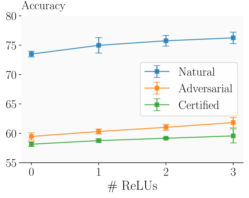
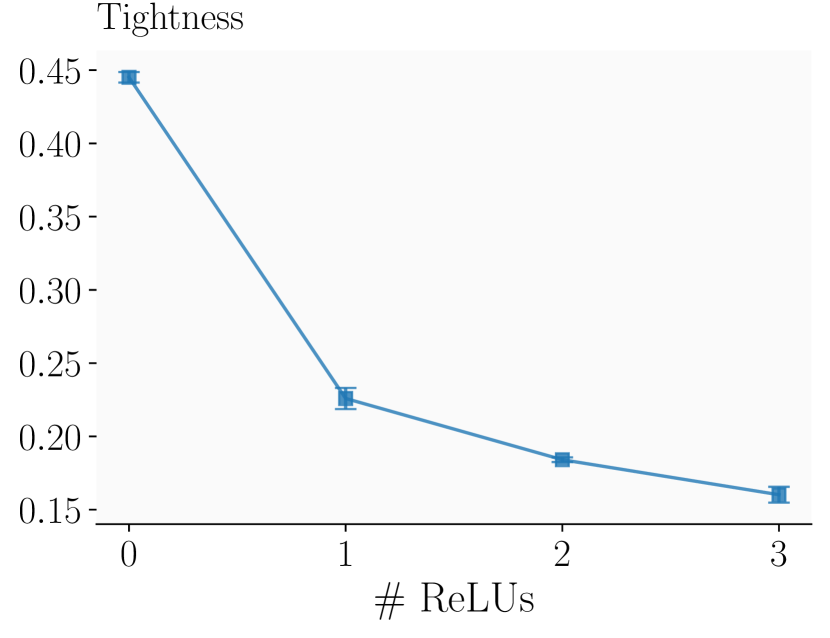
Figure 9: Accuracies and tightness of a CNN7 for CIFAR-10 $\epsilon=\frac{2}{255}$ depending on regularization strength with STAPS

We visualize the result of thus varying regularization levels by changing the number of ReLU layers in the classifier in Figure 9. We observe very similar trends as for SABR in Figure 6, although to a lesser extent, as $0$ ReLU layers in the classifier still recovers SABR and not standard IBP. Again, decreasing regularization (increasing the number of ReLU layers in the classifier) leads to reducing tightness and increasing standard and certified accuracies.

Appendix E Reproducibility

We publish our code, all trained models, and detailed instructions on how to reproduce our results at ANONYMIZED, providing an anonymized version to the reviewers. Further, we provide detailed descriptions of all hyper-parameter choices, data sets, and preprocessing steps in App. C.

References

- Biggio et al. [2013] B. Biggio, I. Corona, D. Maiorca, B. Nelson, N. Srndic, P. Laskov, G. Giacinto, and F. Roli, “Evasion attacks against machine learning at test time,” in Proc of ECML PKDD, vol. 8190, 2013.
- Szegedy et al. [2014] C. Szegedy, W. Zaremba, I. Sutskever, J. Bruna, D. Erhan, I. J. Goodfellow, and R. Fergus, “Intriguing properties of neural networks,” in Proc. of ICLR, 2014.
- Zhang et al. [2022] H. Zhang, S. Wang, K. Xu, L. Li, B. Li, S. Jana, C. Hsieh, and J. Z. Kolter, “General cutting planes for bound-propagation-based neural network verification,” ArXiv preprint, vol. abs/2208.05740, 2022.
- Ferrari et al. [2022] C. Ferrari, M. N. Müller, N. Jovanovic, and M. T. Vechev, “Complete verification via multi-neuron relaxation guided branch-and-bound,” in Proc. of ICLR, 2022.
- Singh et al. [2018] G. Singh, T. Gehr, M. Mirman, M. Püschel, and M. T. Vechev, “Fast and effective robustness certification,” in Proc. of NeurIPS, 2018.
- Singh et al. [2019a] G. Singh, T. Gehr, M. Püschel, and M. T. Vechev, “An abstract domain for certifying neural networks,” Proc. ACM Program. Lang., vol. 3, no. POPL, 2019.
- Gowal et al. [2018] S. Gowal, K. Dvijotham, R. Stanforth, R. Bunel, C. Qin, J. Uesato, R. Arandjelovic, T. A. Mann, and P. Kohli, “On the effectiveness of interval bound propagation for training verifiably robust models,” ArXiv preprint, vol. abs/1810.12715, 2018.
- Shi et al. [2021] Z. Shi, Y. Wang, H. Zhang, J. Yi, and C. Hsieh, “Fast certified robust training with short warmup,” in Proc. of NeurIPS, 2021.
- Jovanović et al. [2022] N. Jovanović, M. Balunović, M. Baader, and M. Vechev, “On the paradox of certified training,” in Transactions on Machine Learning Research, 2022.
- Müller et al. [2022a] M. N. Müller, F. Eckert, M. Fischer, and M. T. Vechev, “Certified training: Small boxes are all you need,” CoRR, vol. abs/2210.04871, 2022.
- Mao et al. [2023] Y. Mao, M. N. Müller, M. Fischer, and M. Vechev, “Taps: Connecting certified and adversarial training,” 2023.
- Palma et al. [2022] A. D. Palma, R. Bunel, K. Dvijotham, M. P. Kumar, and R. Stanforth, “IBP regularization for verified adversarial robustness via branch-and-bound,” ArXiv preprint, vol. abs/2206.14772, 2022.
- Tsipras et al. [2019] D. Tsipras, S. Santurkar, L. Engstrom, A. Turner, and A. Madry, “Robustness may be at odds with accuracy,” in Proc. of ICLR, 2019.
- Mirman et al. [2018] M. Mirman, T. Gehr, and M. T. Vechev, “Differentiable abstract interpretation for provably robust neural networks,” in Proc. of ICML, vol. 80, 2018.
- Tramèr et al. [2020] F. Tramèr, N. Carlini, W. Brendel, and A. Madry, “On adaptive attacks to adversarial example defenses,” in Proc. of NeurIPS, 2020.
- Croce and Hein [2020] F. Croce and M. Hein, “Reliable evaluation of adversarial robustness with an ensemble of diverse parameter-free attacks,” in Proc. of ICML, vol. 119, 2020.
- Zhang et al. [2020] H. Zhang, H. Chen, C. Xiao, S. Gowal, R. Stanforth, B. Li, D. S. Boning, and C. Hsieh, “Towards stable and efficient training of verifiably robust neural networks,” in Proc. of ICLR, 2020.
- Balunovic and Vechev [2020] M. Balunovic and M. T. Vechev, “Adversarial training and provable defenses: Bridging the gap,” in Proc. of ICLR, 2020.
- Wong et al. [2018] E. Wong, F. R. Schmidt, J. H. Metzen, and J. Z. Kolter, “Scaling provable adversarial defenses,” in Proc. of NeurIPS, 2018.
- Saxe et al. [2014] A. M. Saxe, J. L. McClelland, and S. Ganguli, “Exact solutions to the nonlinear dynamics of learning in deep linear neural networks,” in Proc. of ICLR, 2014.
- Ji and Telgarsky [2019] Z. Ji and M. Telgarsky, “Gradient descent aligns the layers of deep linear networks,” in Proc. of ICLR, 2019.
- Wu et al. [2019] L. Wu, Q. Wang, and C. Ma, “Global convergence of gradient descent for deep linear residual networks,” in Proc. of NeurIPS, 2019.
- Ribeiro et al. [2016] M. T. Ribeiro, S. Singh, and C. Guestrin, “"why should I trust you?": Explaining the predictions of any classifier,” in Proceedings of the 22nd ACM SIGKDD International Conference on Knowledge Discovery and Data Mining, San Francisco, CA, USA, August 13-17, 2016, 2016.
- Lin et al. [2022] V. Lin, R. Ivanov, J. Weimer, O. Sokolsky, and I. Lee, “T4V: exploring neural network architectures that improve the scalability of neural network verification,” in Principles of Systems Design - Essays Dedicated to Thomas A. Henzinger on the Occasion of His 60th Birthday, vol. 13660, 2022.
- Chorowski and Zurada [2014] J. Chorowski and J. M. Zurada, “Learning understandable neural networks with nonnegative weight constraints,” IEEE transactions on neural networks and learning systems, vol. 26, no. 1, 2014.
- Glorot and Bengio [2010] X. Glorot and Y. Bengio, “Understanding the difficulty of training deep feedforward neural networks,” in Proc. of AISTATS, vol. 9, 2010.
- He et al. [2015] K. He, X. Zhang, S. Ren, and J. Sun, “Delving deep into rectifiers: Surpassing human-level performance on imagenet classification,” in Proc. of ICCV, 2015.
- Pope et al. [2021] P. Pope, C. Zhu, A. Abdelkader, M. Goldblum, and T. Goldstein, “The intrinsic dimension of images and its impact on learning,” in Proc. of ICLR, 2021.
- Brix et al. [2023] C. Brix, M. N. Müller, S. Bak, T. T. Johnson, and C. Liu, “First three years of the international verification of neural networks competition (VNN-COMP),” CoRR, vol. abs/2301.05815, 2023.
- Müller et al. [2022b] M. N. Müller, C. Brix, S. Bak, C. Liu, and T. T. Johnson, “The third international verification of neural networks competition (VNN-COMP 2022): Summary and results,” CoRR, vol. abs/2212.10376, 2022.
- Bunel et al. [2020] R. Bunel, J. Lu, I. Turkaslan, P. H. S. Torr, P. Kohli, and M. P. Kumar, “Branch and bound for piecewise linear neural network verification,” J. Mach. Learn. Res., vol. 21, 2020.
- Müller et al. [2022c] M. N. Müller, G. Makarchuk, G. Singh, M. Püschel, and M. T. Vechev, “PRIMA: general and precise neural network certification via scalable convex hull approximations,” Proc. ACM Program. Lang., vol. 6, no. POPL, 2022.
- Singh et al. [2019b] G. Singh, R. Ganvir, M. Püschel, and M. T. Vechev, “Beyond the single neuron convex barrier for neural network certification,” in Proc. of NeurIPS, 2019.
- Wong and Kolter [2018] E. Wong and J. Z. Kolter, “Provable defenses against adversarial examples via the convex outer adversarial polytope,” in Proc. of ICML, vol. 80, 2018.
- Baader et al. [2020] M. Baader, M. Mirman, and M. T. Vechev, “Universal approximation with certified networks,” in Proc. of ICLR, 2020.
- Wang et al. [2022a] Z. Wang, A. Albarghouthi, G. Prakriya, and S. Jha, “Interval universal approximation for neural networks,” Proc. ACM Program. Lang., vol. 6, no. POPL, 2022.
- Wang et al. [2022b] Y. Wang, Z. Shi, Q. Gu, and C. Hsieh, “On the convergence of certified robust training with interval bound propagation,” in Proc. of ICLR, 2022.
- Mirman et al. [2022] M. B. Mirman, M. Baader, and M. Vechev, “The fundamental limits of neural networks for interval certified robustness,” Transactions on Machine Learning Research, 2022.
- Cook [1957] J. Cook, “Rational formulae for the production of a spherically symmetric probability distribution,” Mathematics of Computation, vol. 11, no. 58, 1957.
- Marsaglia [1972] G. Marsaglia, “Choosing a point from the surface of a sphere,” The Annals of Mathematical Statistics, vol. 43, no. 2, 1972.
- Pinelis and Molzon [2016] I. Pinelis and R. Molzon, “Optimal-order bounds on the rate of convergence to normality in the multivariate delta method,” 2016.
- LeCun et al. [2010] Y. LeCun, C. Cortes, and C. Burges, “Mnist handwritten digit database,” ATT Labs [Online]. Available: http://yann.lecun.com/exdb/mnist, vol. 2, 2010.
- Krizhevsky et al. [2009] A. Krizhevsky, G. Hinton et al., “Learning multiple layers of features from tiny images,” 2009.