A normal form for bases of
finite-dimensional vector spaces

Abstract

Most algorithms constructing bases of finite-dimensional vector spaces return basis vectors which, apart from orthogonality, do not show any special properties. While every basis is sufficient to define the vector space, not all bases are equally suited to unravel properties of the problem to be solved. In this paper a normal form for bases of finite-dimensional vector spaces is introduced which may prove very useful in the context of understanding the structure of the problem in which the basis appears in a step towards the solution. This normal form may be viewed as a new normal form for matrices of full column rank.

1 Motivation

Consider the following simple mathematical problem: Find a basis of the four-dimensional vector space $V\subset W\simeq\mathbbm{R}^{5}$ orthogonal to the vector $a=(1,1,1,1,1)^{\text{T}}\in W$. Numerically, an answer to this problem can be found by computing a basis of the kernel (nullspace) of $a^{\text{T}}$. For example, Octave [1], using the command null, returns the following basis, denoted as columns of a matrix:

$$\left(\begin{matrix}[r]-0.44721&-0.44721&-0.44721&-0.44721\\ 0.86180&-0.13820&-0.13820&-0.13820\\ -0.13820&0.86180&-0.13820&-0.13820\\ -0.13820&-0.13820&0.86180&-0.13820\\ -0.13820&-0.13820&-0.13820&0.86180\end{matrix}\right).$$ (1)

To numerical accuracy this basis is a correct solution. Moreover, it is an orthogonal basis. It is, however, not the answer a human would give. A human may give an answer like

$$\left(\begin{matrix}[r]1&0&0&0\\ -1&1&0&0\\ 0&-1&1&0\\ 0&0&-1&1\\ 0&0&0&-1\end{matrix}\right).$$ (2)

While the two bases of Eqs. (1) and (2) span the same vector space, the second one appears to be simpler and more suited for the human mind to grasp the properties of the solution. The basis in Eq. (2) has the following properties:

1. Orthogonality to $a$ is evident without any computational aid (pen and paper, computer).

2. Any basis vector can be characterised by two non-zero entries.

3. Having seen the solution in this form, the solution can immediately be generalised to the corresponding problem in $\mathbbm{R}^{n}$.

Point 2 above may be of crucial importance given the fact that in the context of a scientific or technical application the elements of the involved vector spaces may have a specific physical meaning. At this point it is important to remember that the numerical notation of the vectors above is shorthand for

$$a=\left(\begin{matrix}[r]a_{1}\\ a_{2}\\ a_{3}\\ a_{4}\\ a_{5}\end{matrix}\right)\equiv\sum_{i=1}^{5}a_{i}w_{i},$$ (3)

where the $w_{i}$ are fixed basis vectors of $W$ chosen to describe the problem in an appropriate way. Each of the $w_{i}$ may in general describe an individual physical quantity. For example, the $w_{i}$ could represent measurements from five different devices. If this is the case, each basis vector in Eq. (2) involves a minimal number (two in the shown example) of quantities, while the basis vectors of Eq. (1) combine all involved quantities in each basis vector.

The situation exemplified above may be faced in any situation which involves the solution of a linear equation

$$Mx=y,$$ (4)

where $M\in\mathbbm{R}^{m\times n}$ is an $m\times n$-matrix of full row rank $m$ ($m<n$) and $x\in\mathbbm{R}^{n}$, $y\in\mathbbm{R}^{m}$ are column vectors. The general solution of this linear underdetermined system is given by

$$x=x_{p}+\sum_{i=1}^{n-m}\lambda_{i}k_{i},$$ (5)

where $x_{p}$ is a particular solution of Eq. (4), $k_{1},\ldots,k_{n-m}\in\mathbbm{R}^{n}$ form a basis of the kernel $\mathrm{ker}\,M$ and $\lambda_{1},\ldots,\lambda_{n-m}\in\mathbbm{R}$ are free coefficients. The choice of basis of $\mathrm{ker}\,M$ is not restricted, and regarding the parameterisation of the solution (5) each basis is equivalent. Since, however, $\mathrm{ker}\,M\subset\mathbbm{R}^{n}$ is embedded into an $n$-dimensional vector space where each of the $n$ directions may have a different physical meaning, some bases of $\mathrm{ker}\,M$ may be more expressive or suited to the problem than others.

The outline of this paper is as follows. In Section 2 a normal form for bases of finite-dimensional vector spaces is defined. The practical use of this normal form is demonstrated by sample applications in Section 3. Finally, Section 4 concludes the paper.

2 Definition of a normal form for bases of finite-dimensional vector spaces

In the following, a definition of a normal form for a basis of a finite-dimensional vector space $V\subseteq\mathbbm{F}^{m}$ with $\mathbbm{F}=\mathbbm{R}$ or $\mathbbm{C}$ is given. It has been developed with the following goals in mind:

• Existence for any vector space $V\subseteq\mathbbm{F}^{m}$ of dimension $n=\mathrm{dim}\,V\geq 2$.

• Uniqueness.

• A high number of zero entries in the basis vectors.

• If $\mathrm{dim}V=m$, the basis in normal form shall consist of the columns of the $m\times m$ unit matrix.

Given:

An $m\times n$-matrix

$$A=\begin{pmatrix}c_{1},\ldots,c_{n}\end{pmatrix}=\begin{pmatrix}r_{1}\\ \vdots\\ r_{m}\end{pmatrix}\in\mathbbm{F}^{m\times n}$$ (6)

of full column rank $n\leq m$. The columns $c_{1},\ldots,c_{n}$ represent the basis vectors of the $n$-dimensional vector space $V\subseteq\mathbbm{F}^{m}$ for which a basis in normal form shall be constructed. To avoid trivial cases, $n\geq 2$ is assumed.

Let $R=\{r_{1},\ldots,r_{m}\}$ be the set of rows of $A$. Consider now all selections $S\subset R$ of rows s.t. the selected rows span a vector space of dimension $n-1$, i.e.

$$\mathrm{dim}\;\mathrm{span}(S)=n-1.$$ (7)

Each of the vector spaces $\mathrm{span}(S)\subset\mathbbm{F}^{n}$, geometrically is an $(n-1)$-dimensional hyperplane through $0$ which contains the selected row vectors. Let $s\neq 0$ be a normal vector of this hyperplane, i.e. $r\cdot s=0\;\forall r\in S$. Then $As\in\mathbbm{F}^{m}$ contains at least $|S|$ zero entries. Since $s\neq 0$ and $A$ has full column rank, $As$ has at least one non-vanishing entry. Therefore, the normal vector $s$ can be made unique by requiring that the first non-vanishing element of $As$ shall be $+1$. In the following, the normal vectors $\hat{s}$ normalised s.t. they fulfil this requirement are denoted with a hat. In this way, each selection $S$ is assigned a unique vector $\hat{s}\in\mathbbm{F}^{n}$.

Lemma 1.

The set of all normal vectors $\hat{s}\in\mathbbm{F}^{n}$ to all selections $S$ is a generating set of $\mathbbm{F}^{n}$.

Proof.

This can be proven by explicitly constructing $n$ linearly independent vectors $\hat{s}$. Since $A$ has full column rank $n$, one can select $n$ linearly independent rows $\rho_{1},\ldots,\rho_{n}$ of $A$. From these, one can form the $n$ different selections

$$S_{i}=\{\rho_{1},\ldots,\rho_{i-1},\rho_{i+1},\ldots,\rho_{n}\}.$$ (8)

Each of the $S_{i}$ spans an $(n-1)$-dimensional vector space. The $i$-th column of

$$\rho^{-1}\equiv\begin{pmatrix}\rho_{1}\\ \vdots\\ \rho_{n}\end{pmatrix}^{-1}$$ (9)

is a normal vector of $\mathrm{span}(S_{i})$. Therefore, the $n$ linearly independent columns of $\rho^{-1}$ provide $n$ linearly independent vectors $s$. Normalisation of these yields $n$ linearly independent vectors $\hat{s}$. ∎

The vectors $\hat{s}$ will be used to define the normal form. The main idea of this definition is to order all possible $\hat{s}$ w.r.t. the number of zero entries they generate in $A\hat{s}$. For the same number of zeros, those $A\hat{s}$ shall be preferred for which the zero entries have higher indices. For example,

$$\begin{pmatrix}0\\ 0\\ 1\\ \times\end{pmatrix}\quad\text{shall be preferred over}\quad\begin{pmatrix}1\\ \times\\ \times\\ 0\end{pmatrix}$$ (10)

and

$$\begin{pmatrix}1\\ \times\\ 0\\ \times\end{pmatrix}\quad\text{over}\quad\begin{pmatrix}0\\ 1\\ \times\\ \times\end{pmatrix}.$$ (11)

The symbol $\times$ here denotes an arbitrary non-zero entry. This ordering will be formally defined by assigning each vector $\hat{s}$ an integer number.

Definition 1.

Let $\hat{s}$ be the normal vector to the hyperplane $\mathrm{span}(S)$, then define

$$\theta^{(1)}(\hat{s})\equiv 2^{m+\sum_{j=1}^{m}\theta_{j}},$$ (12)

$$\theta^{(2)}(\hat{s})\equiv\sum_{j=1}^{m}\theta_{j}2^{j-1},$$ (13)

where

$$\theta_{j}=\begin{cases}1&\text{for $(A\hat{s})_{j}=0$}\\ 0&\text{else}.\end{cases}$$ (14)

The first term $\theta^{(1)}(\hat{s})$ is larger than the maximal value $\theta^{(2)}$ can assume (which is $2^{m}-2$ if all entries of $A\hat{s}$ except the first one are zero) and encodes the total number of zeros in $A\hat{s}$. The second term describes the preference for zero entries with higher indices. Therefore, the number

$$\theta(\hat{s})\equiv\theta^{(1)}(\hat{s})+\theta^{(2)}(\hat{s})$$ (15)

is consistent with the ordering for $\hat{s}$ sketched above. Note that $\theta(\hat{s})$ equals the binary number $(10\ldots 0\theta_{m}\theta_{m-1}\theta_{m-2}\cdots\theta_{2}\theta_{1})_{2}$, where the first digit 1 encodes $\theta^{(1)}(\hat{s})$. The following properties of $\theta(\hat{s})$ are important:

• The encoding of the information which elements of $A\hat{s}$ vanish as the number $\theta(\hat{s})$ is bijective.

• Different $\hat{s}$ correspond to different hyperplanes and thus to different sets of vanishing elements of $A\hat{s}$. Since the encoding is bijective, this means that different $\hat{s}$ are assigned different $\theta(\hat{s})$.

• By definition of $S$, the set of rows orthogonal to $\hat{s}$ contains $n-1$ linearly independent vectors, and thus unambiguously defines $\hat{s}$. But two different selections $S_{1}$, $S_{2}$ of rows of $A$ can correspond to the same $\hat{s}$ and thus to the same $\theta(\hat{s})$. This is the case if and only if

  $$\mathrm{span}(S_{1})=\mathrm{span}(S_{2}).$$ (16)

  A simple example illustrating this is the matrix

  $$A=\left(\begin{matrix}r_{1}\\ r_{2}\\ r_{3}\end{matrix}\right)=\left(\begin{matrix}1&0\\ 0&1\\ 2&0\end{matrix}\right)$$ (17)

  with the three possible selections $S_{1}=\{r_{1}\}$, $S_{2}=\{r_{2}\}$, $S_{3}=\{r_{3}\}$. Though $S_{1}$ and $S_{3}$ are different, they correspond to the same $\hat{s}\equiv(0,\,1)^{\mathrm{T}}$. The $\hat{s}$ of $S_{2}$ is $\hat{s}^{\prime}\equiv(1,\,0)^{\mathrm{T}}$. From

  $$A\hat{s}=\left(\begin{matrix}0\\ 1\\ 0\end{matrix}\right)\text{ and }A\hat{s}^{\prime}=\left(\begin{matrix}1\\ 0\\ 2\end{matrix}\right)$$ (18)

  one finds

  $$\theta(\hat{s})=2^{3+2}+2^{0}+2^{2}=37\text{ and }\theta(\hat{s}^{\prime})=2^{3+1}+2^{1}=18.$$ (19)

Since different $\hat{s}$ are assigned different $\theta(\hat{s})$, the numbers can be used to order the set of all normal vectors $\hat{s}$ constructed from all selections $S$.

Definition 2.

Let $\mathcal{S}$ be the set of all different normal vectors $\hat{s}$ to all selections $S\subset R$. Then define

$$\hat{s}_{1}\equiv\underset{\hat{s}\in\mathcal{S}}{\mathrm{argmax}}\,\theta(\hat{s}),$$ (20a)

$$\hat{s}_{j}\equiv\underset{\hat{s}\in\mathcal{S}_{j}}{\mathrm{argmax}}\,\theta(\hat{s}),\;j\in\{2,\ldots,n\},$$ (20b)

where

$$\mathcal{S}_{j}\equiv\{\hat{s}\in\mathcal{S}|\text{$\hat{s}$ linearly independent of $\hat{s}_{1},\ldots,\hat{s}_{j-1}$}\}.$$ (21)

The normal form of the basis specified by the columns $\{c_{1},\ldots,c_{n}\}$ of $A$ is defined as the set of column vectors

$$\{A\hat{s}_{1},\ldots A\hat{s}_{n}\}.$$ (22)

Theorem 1.

The normal form exists and is unique for all matrices $A$ of Eq. (6), i.e. all vector spaces $V\subset\mathbbm{F}^{m}$ of dimension $n\geq 2$. If $n=m$, i.e. if $A$ is a square matrix, the normal form of $A$ is given by the $m\times m$ unit matrix.

Proof.

From Lemma 1 it follows that there are $n$ linearly independent vectors $\hat{s}$. Since all $\hat{s}$ are mapped to different $\theta(\hat{s})$, the maximisations of Definition 2 all have unique solutions. Therefore, the normal form exists and is unique. In the special case of a square matrix $A$, there are only $m$ different selections $S$ of rows of $A$ and the corresponding vectors $\hat{s}$ must be the columns of $A^{-1}$—see the proof of Lemma 1—and one has

$$A(\hat{s}_{1},\ldots,\hat{s}_{m})=AA^{-1}=\mathbbm{1}_{m}.$$ (23)

The vectors $\hat{s}_{1},\ldots\hat{s}_{m}$ according to this equation are ordered as in Eq. (20) because

$$\theta(\hat{s}_{j})=2^{2m-1}+2^{m}-1-2^{j-1}>\theta(\hat{s}_{j+1}).$$ (24)

∎

3 Example applications

The following subsections illustrate the use of the normal form in examples from different areas of physics and mathematics. All numerical computations of the normal form have been carried out using the implementation provided in appendix B.

3.1 Basis of a space orthogonal to a vector

As a first example consider the basis in Eq. (1) of the vector space $V$ orthogonal to $a=(1,1,1,1,1)^{\text{T}}$. In normal form the basis is given by

$$\left(\begin{matrix}[r]1&1&1&1\\ -1&0&0&0\\ 0&-1&0&0\\ 0&0&-1&0\\ 0&0&0&-1\end{matrix}\right),$$ (25)

which shows the same desirable properties as the basis in Eq. (2) which was the motivation for the need of a normal form. This may be generalised to an arbitrary $a\in\mathbbm{F}^{m}$, provided $a_{i}\neq 0\,\forall i\in\{1,\ldots,m\}$. Then the normal form is given by

$$\left(\begin{matrix}[r]1&1&\cdots&1\\ -a_{1}/a_{2}&0&&0\\ 0&-a_{1}/a_{3}&&0\\ 0&0&&0\\ \vdots&\vdots&&\vdots\\ 0&0&\cdots&-a_{1}/a_{m}\end{matrix}\right)$$ (26)

or, in terms of the basis vectors $v_{1},\ldots,v_{m-1}$ of $\mathrm{ker}(a^{\mathrm{T}})$,

$$(v_{i})_{j}=\begin{cases}1&\text{for }j=1\\ -a_{1}/a_{j}&\text{for }j=i+1\\ 0&\text{else}.\end{cases}$$ (27)

Also for the case of a vector space $V$ orthogonal to two vectors $a_{1}$, $a_{2}\in\mathbbm{F}^{m}$ an analytic expression for the basis in normal form can be given. Note that the expression constructed in the following is not valid in all cases. Nevertheless its derivation serves as a good illustration for the general structure of the normal form and special cases to be taken care of. As for the one-dimensional case, the first row of the normal form in the general case will consist of one entries only. Then, according to the requirement of putting the zero entries as low as possible, also the second row in general will be non-zero and the remainder of the $m\times m-2$-matrix of basis vectors will be diagonal, i.e.

$$\left(\begin{matrix}[c]1&1&\cdots&1\\ \times&\times&\cdots&\times\\ \times&0&&0\\ 0&\times&&0\\ \vdots&\vdots&&\vdots\\ 0&0&\cdots&\times\end{matrix}\right),$$ (28)

where $\times$ denotes a non-zero entry. From the requirements $v_{i}\cdot a_{1}=0$ and $v_{i}\cdot a_{2}=0$ for the basis vectors $v_{i}$ in normal form then follows

$$(v_{i})_{j}=\begin{cases}1&\text{for }j=1\\ v^{(i)}&\text{for }j=2\\ v^{(i)\prime}&\text{for }j=i+2\\ 0&\text{else}\end{cases}$$ (29)

with

$$\begin{pmatrix}v^{(i)}\\ v^{(i)\prime}\end{pmatrix}=-\begin{pmatrix}(a_{1})_{2}&(a_{1})_{i+2}\\ (a_{2})_{2}&(a_{2})_{i+2}\end{pmatrix}^{-1}\begin{pmatrix}(a_{1})_{1}\\ (a_{2})_{1}\end{pmatrix}.$$ (30)

This result has been tested numerically with real and complex random vectors $a_{1}$ and $a_{2}$ up to dimension 20. However, Eqs. (28) and (29) can only hold if the $2\times 2$-matrix in Eq. (30) is invertible for all $i\in\{1,\ldots,m-2\}$. Moreover, in order to describe a basis, the matrix of Eq. (28) must not contain more than two vanishing (or three linearly dependent) rows. Thus, if all $v^{(i)}$ were equal, at most one of the $v^{(i)\prime}$ could be zero. And if the $v^{(i)}$ are not all equal, at most two of the $v^{(i)\prime}$ can be zero. Otherwise, the normal form will not be given by Eq. (29) and one has to resort to Definition 2 to compute the normal form. Appendix A provides an algorithm to compute the normal form which is valid for all cases.

3.2 Dimensional analysis

The main statement of dimensional analysis [2, 3] can be summarised as: If a physical quantity $q$ can be expressed as a function of other physical quantities $q_{1},\ldots q_{n}$, then this function assumes the form

$$q=\tilde{q}\times f(a_{1},\ldots,a_{m}),$$ (31)

where $\tilde{q}$ is a product of powers of $q_{1},\ldots,q_{n}$ of the physical dimension of $q$ and $\{a_{1},\ldots,a_{m}\}$ is a set of independent dimensionless products of powers of $q_{1},\ldots,q_{n}$.

As an example consider the equation of motion of a one-dimensional harmonic oscillator

$$m\ddot{x}=-kx,\quad x(0)=x_{0},\quad\dot{x}(0)=\dot{x}_{0}.$$ (32)

The position $x(t)$ of the oscillator must then be a function of $t,x_{0},\dot{x}_{0},k$ and $m$. Applying dimensional analysis to this problem one finds

$$x(t)=x_{0}\times f(a_{1},\ldots,a_{m}),$$ (33)

where $x_{0}$ has been chosen as a quantity of the same dimension as $x(t)$. A complete set of independent dimensionless products of powers $\{a_{1},\ldots,a_{m}\}$ can be found by means of the matrix [2, 3]

$$B=\blockarray{cccccc}&tx_{0}\dot{x}_{0}km\\ \block{l(rrrrr)}M00011\\ L01100\\ T10-1-20\\ \;.$$ (34)

The rows of $B$ encode the dimensions $M,L,T=$ mass, length, time and the columns the five physical quantities the sought-for $x(t)$ depends on. The matrix entries are the powers of $M,L,T$ in the physical dimensions of $t,x_{0},\dot{x}_{0},k,m$. A maximal set of independent dimensionless products of powers $a_{1},\ldots a_{m}$ can then be found by constructing the basis of $\mathrm{ker}\,B$ [2, 3]. Doing so via singular value decomposition of $B$ using the NumPy package [4] one finds that $\mathrm{ker}\,B$ is spanned by the columns of

$$\left(\begin{matrix}[r]-0.35314643&-0.76783678\\ 0.64522571&-0.11070323\\ -0.64522571&0.11070323\\ 0.14603964&-0.43927000\\ -0.14603964&0.43927000\end{matrix}\right).$$ (35)

The normal form of this basis is given by

$$\left(\begin{matrix}[r]1&1\\ -1&0\\ 1&0\\ 0&1/2\\ 0&-1/2\end{matrix}\right).$$ (36)

A set of independent dimensionless products of powers of $t,x_{0},\dot{x}_{0},k,m$ is thus given by

$$a_{1}=\frac{t\dot{x}_{0}}{x_{0}},\quad a_{2}=\sqrt{\frac{k}{m}}t.$$ (37)

According to dimensional analysis, the solution of the equation of motion of the oscillator must therefore assume the form

$$x(t)=x_{0}\times f(a_{1},a_{2}).$$ (38)

Indeed, the solution

$$\begin{split}x(t)&=x_{0}\cos(\omega t)+\frac{\dot{x}_{0}}{\omega}\sin(\omega t)=x_{0}\times\left(\cos(\omega t)+\frac{t\dot{x}_{0}}{x_{0}}\frac{1}{\omega t}\sin(\omega t)\right)=\\ &=x_{0}\times\left(\cos(a_{2})+\frac{a_{1}}{a_{2}}\sin(a_{2})\right),\end{split}$$ (39)

with $\omega\equiv\sqrt{k/m}$ is of the form of Eq. (38).

In this example, the normal form allows to formulate the solution of a physical problem in a particularly simple form. The reason for this simplicity is that in normal form the dimensionless products of powers $a_{i}$ depend on as few physical quantities as possible. The idea to use the freedom of basis choice for this purpose has for example been applied in the symbolic regression technique AI Feynman [5].

3.3 Numerical application of Noether’s theorem

In its simplest form Noether’s theorem [6] states that for every differentiable one-parametric symmetry transformation of the Lagrangian (to be more precise: the action integral) of a system, there is a corresponding conserved quantity. In the following, the case of a Lagrangian $L(x(t),\dot{x}(t))$ invariant under a one-parametric transformation $x(t)\mapsto x_{\lambda}(t)$ with $x_{\lambda}(t)|_{\lambda=0}=x(t)$ is considered. Due to the invariance

$$L(x_{\lambda}(t),\dot{x}_{\lambda}(t))=L(x(t),\dot{x}(t))$$ (40)

one finds

$$\begin{split}0&=\frac{d}{d\lambda}\Big{|}_{\lambda=0}L(x_{\lambda}(t),\dot{x}_{\lambda}(t))=\frac{\partial L}{\partial x}\frac{\partial x_{\lambda}}{\partial\lambda}\Big{|}_{\lambda=0}+\frac{\partial L}{\partial\dot{x}}\frac{\partial\dot{x}_{\lambda}}{\partial\lambda}\Big{|}_{\lambda=0}\\ &=\frac{\partial L}{\partial x}\frac{\partial x_{\lambda}}{\partial\lambda}\Big{|}_{\lambda=0}+\frac{\partial L}{\partial\dot{x}}\frac{d}{dt}\frac{\partial x_{\lambda}}{\partial\lambda}\Big{|}_{\lambda=0}\\ &=\underbrace{\left(\frac{\partial L}{\partial x}-\frac{d}{dt}\frac{\partial L}{\partial\dot{x}}\right)}_{0}\frac{\partial x_{\lambda}}{\partial\lambda}\Big{|}_{\lambda=0}+\frac{d}{dt}\left(\frac{\partial L}{\partial\dot{x}}\frac{\partial x_{\lambda}}{\partial\lambda}\right)\Big{|}_{\lambda=0}\\ &=\frac{d}{dt}\left(\frac{\partial L}{\partial\dot{x}}\frac{\partial x_{\lambda}}{\partial\lambda}\right)\Big{|}_{\lambda=0},\end{split}$$ (41)

where in the last step the Euler-Lagrange equation has been used. For an infinitesimal symmetry transformation of the form

$$x_{\lambda}(t)=x(t)+\lambda(a+Bx(t))+O(\lambda)^{2}$$ (42)

the conserved quantity is thus given by

$$\frac{\partial L}{\partial\dot{x}}(a+Bx(t)).$$ (43)

In the following, the normal form for bases will be shown to provide an elegant way to numerically apply Noether’s theorem to symmetry transformations of this form.

To find all symmetry transformations of the form of Eq. (42), expand $L(x_{\lambda}(t),\dot{x}_{\lambda}(t))$ into a Taylor series around $\lambda=0$.

$$L(x_{\lambda},\dot{x}_{\lambda})=L(x,\dot{x})+\lambda\left(\frac{\partial L}{\partial x}(a+Bx)+\frac{\partial L}{\partial\dot{x}}B\dot{x}\right)+O(\lambda^{2}).$$ (44)

The transformation is a symmetry transformation if

$$\frac{\partial L}{\partial x}(a+Bx)+\frac{\partial L}{\partial\dot{x}}B\dot{x}=0\quad\forall x,\dot{x}.$$ (45)

This provides a set of (infinitely many) linear equations for $a$ and $B$. Let the coordinate vector $x$ have $p$ components, i.e. $x\in\mathbbm{R}^{p}$. Then, defining

$$\mathcal{D}L\equiv\begin{pmatrix}\frac{\partial L}{\partial x_{1}},\ldots,\frac{\partial L}{\partial x_{p}},\frac{\partial L}{\partial x_{1}}x_{1}+\frac{\partial L}{\partial\dot{x}_{1}}\dot{x}_{1},\frac{\partial L}{\partial x_{1}}x_{2}+\frac{\partial L}{\partial\dot{x}_{1}}\dot{x}_{2},\ldots\frac{\partial L}{\partial x_{p}}x_{p}+\frac{\partial L}{\partial\dot{x}_{p}}\dot{x}_{p}\end{pmatrix},$$ (46)

and

$$A\equiv\begin{pmatrix}a_{1},\ldots,a_{p},B_{11},B_{12},\ldots B_{pp}\end{pmatrix}^{\mathrm{T}},$$ (47)

the equations (45) can be written as

$$\mathcal{D}L(x,\dot{x})A=0\quad\forall x,\dot{x}.$$ (48)

The possible values for $A$ can thus be found by constructing a basis of the common kernel

$$\bigcap_{x,\dot{x}}\;\mathrm{ker}\,\mathcal{D}L(x,\dot{x}).$$ (49)

This common kernel can be found numerically by choosing $\nu$ random values for $x$ and $\dot{x}$. Combining the obtained random $\mathcal{D}L(x,\dot{x})$ to a $\nu\times(p+p^{2})$-matrix, a basis of the common kernel is given by a basis of the kernel of the matrix. If there are symmetry transformations of the proposed form, this procedure for a sufficiently high $\nu$ will lead to a non-trivial common kernel valid for all $x$ and $\dot{x}$.

As an example consider the two-body problem in three dimensions with a $1/r$ potential:

$$L(\vec{x}_{1},\vec{x}_{2},\dot{\vec{x}}_{1},\dot{\vec{x}}_{2})=\frac{1}{2}m_{1}\dot{\vec{x}}_{1}^{2}+\frac{1}{2}m_{2}\dot{\vec{x}}_{2}^{2}+\frac{\alpha}{|\vec{x}_{1}-\vec{x}_{2}|}.$$ (50)

With $\vec{r}\equiv\vec{x}_{1}-\vec{x}_{2}$ and $r\equiv|\vec{r}|$, the derivatives needed for Eq. (46) are

$$\frac{\partial L}{\partial(\vec{x}_{1})_{i}}=-\frac{\alpha r_{i}}{r^{3}},\quad\frac{\partial L}{\partial(\vec{x}_{2})_{i}}=+\frac{\alpha r_{i}}{r^{3}},\quad\frac{\partial L}{\partial(\dot{\vec{x}}_{1})_{i}}=m_{1}(\dot{\vec{x}}_{1})_{i},\quad\frac{\partial L}{\partial(\dot{\vec{x}}_{2})_{i}}=m_{2}(\dot{\vec{x}}_{2})_{i}$$ (51)

for $i=1,2,3$. The vector $\mathcal{D}L$ in this example has dimension $6+6^{2}=42$. Assigning $m_{1},m_{2},\alpha$ fixed numerical values $\in[0,1]$ (the exact values are not relevant, however, $m_{1}\neq m_{2}$ is important) and subsequently assigning $\vec{x}_{1}$, $\vec{x}_{2}$, $\dot{\vec{x}}_{1}$, $\dot{\vec{x}}_{2}$ different random values in $[0,1]^{3}$, and computing the common kernel of all resulting values for $\mathcal{D}L$, a nine-dimensional common kernel is found. Numerically, the basis of this kernel is given by a $42\times 9$-matrix. In the performed numerical experiment, 12 of the 42 rows of this matrix vanished, the others, however, were densely populated with non-zero entries. The normal form of the basis is given by a $42\times 9$-matrix with only 36 non-zero entries. The found basis and its normal form are visualised in Fig. 1.

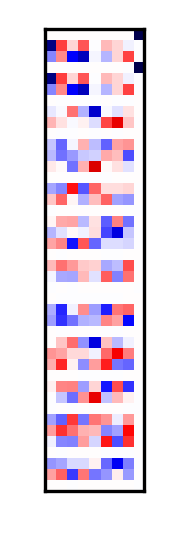
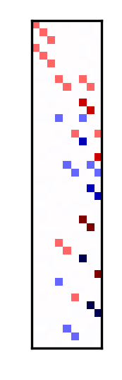
Figure 1: The numerically found basis of the common kernel Eq. (49) (left) and its normal form (right). The coloured fields indicate the values of the matrix entries, white representing a vanishing entry.

In terms of $a$ and $B$, the nine basis vectors in normal form are given by

$$a_{1}=\begin{pmatrix}1&0&0&1&0&0\end{pmatrix}^{\mathrm{T}},\quad B_{1}=0,$$ (52a)

$$a_{2}=\begin{pmatrix}0&1&0&0&1&0\end{pmatrix}^{\mathrm{T}},\quad B_{2}=0,$$ (52b)

$$a_{3}=\begin{pmatrix}0&0&1&0&0&1\end{pmatrix}^{\mathrm{T}},\quad B_{3}=0,$$ (52c)

$$a_{4}=0,\quad B_{4}=\begin{pmatrix}T_{3}&0\\ 0&T_{3}\end{pmatrix},$$ (52d)

$$a_{5}=0,\quad B_{5}=\begin{pmatrix}T_{2}&0\\ 0&T_{2}\end{pmatrix},$$ (52e)

$$a_{6}=0,\quad B_{6}=\begin{pmatrix}T_{1}&0\\ 0&T_{1}\end{pmatrix},$$ (52f)

$$a_{7}=0,\quad B_{7}=\begin{pmatrix}T_{3}&\beta T_{3}\\ (1+\beta)T_{3}&0\end{pmatrix},$$ (52g)

$$a_{8}=0,\quad B_{8}=\begin{pmatrix}T_{2}&\beta T_{2}\\ (1+\beta)T_{2}&0\end{pmatrix},$$ (52h)

$$a_{9}=0,\quad B_{9}=\begin{pmatrix}T_{1}&\beta T_{1}\\ (1+\beta)T_{1}&0\end{pmatrix},$$ (52i)

where

$$\beta\equiv\frac{m_{2}}{m_{1}-m_{2}}=\frac{1}{\frac{m_{1}}{m_{2}}-1}$$ (53)

and

$$T_{1}=\begin{pmatrix}0&0&0\\ 0&0&1\\ 0&-1&0\end{pmatrix},\quad T_{2}=\begin{pmatrix}0&0&1\\ 0&0&0\\ -1&0&0\end{pmatrix},\quad T_{3}=\begin{pmatrix}0&1&0\\ -1&0&0\\ 0&0&0\end{pmatrix}$$ (54)

are the generators of infinitesimal rotations about the three axes. Note that in the numerical experiment described above, $\beta$ is of course represented by a specific floating point number. From dimensional analysis ($B$ is dimensionless) and repeating the experiment for different values assigned to $m_{1}$ and $m_{2}$ the functional form Eq. (53) of $\beta$ can be inferred.

The physical interpretation of six of these nine symmetry transformations is straight forward. The first three correspond to translations in the directions of the three axes in space and the corresponding conserved quantities, cf. Eq. (43), are the components of the total momentum $\vec{p}=m_{1}\dot{\vec{x}}_{1}+m_{2}\dot{\vec{x}}_{2}$. The symmetry transformations number 4 to 6 correspond to rotations about the three axes through the origin, resulting in conservation of the total angular momentum $\vec{L}=m_{1}\vec{x}_{1}\times\dot{\vec{x}}_{1}+m_{2}\vec{x}_{2}\times\dot{\vec{x}}_{2}$.

The remaining three symmetry transformations 7 to 9 are unusual in the sense that they mix the coordinates of the two bodies, i.e. the matrices $B_{7}$ to $B_{9}$ are not block-diagonal. They can, however, be simultaneously block-diagonalised by changing to center-of-mass and relative coordinates, i.e.

$$\begin{pmatrix}\vec{x}_{\text{CM}}\\ \vec{r}\end{pmatrix}\equiv\begin{pmatrix}\frac{m_{1}}{m_{1}+m_{2}}\vec{x}_{1}+\frac{m_{2}}{m_{1}+m_{2}}\vec{x}_{2}\\ \vec{x}_{1}-\vec{x}_{2}\end{pmatrix}=\begin{pmatrix}\frac{1+\beta}{1+2\beta}\mathbbm{1}&\frac{\beta}{1+2\beta}\mathbbm{1}\\ \mathbbm{1}&-\mathbbm{1}\end{pmatrix}\begin{pmatrix}\vec{x}_{1}\\ \vec{x}_{2}\end{pmatrix}.$$ (55)

In these new coordinates, the matrices $B_{7}$ to $B_{9}$ become

$$\begin{pmatrix}(1+\beta)T&0\\ 0&-\beta T\end{pmatrix}\quad\text{with}\quad T=T_{3},T_{2},T_{1}.$$ (56)

Thus, the corresponding symmetry transformations are infinitesimal rotations of the center of mass $\vec{x}_{\text{CM}}$ about the origin and a simultaneous rotation (in general about a different angle) of $\vec{r}$. This can be seen graphically in Fig. 2, where orbits of the finite transformation $\lambda\mapsto\exp(\lambda B_{7})x_{0}$ are shown.

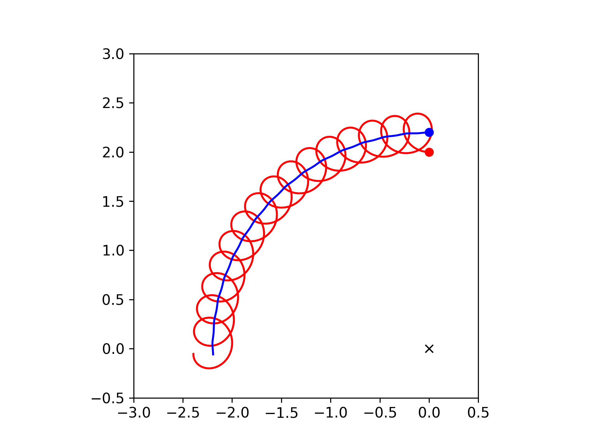
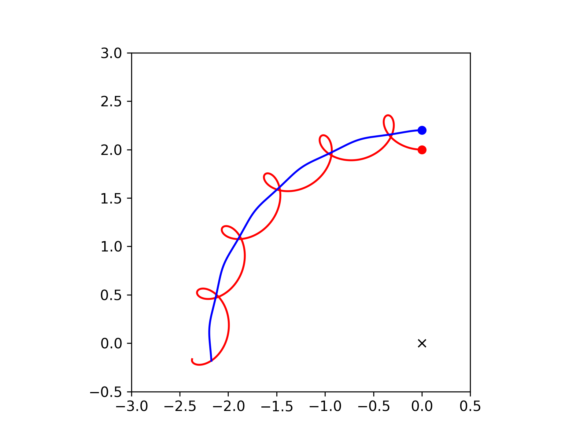
Figure 2: Orbits $\lambda\mapsto\exp(\lambda B_{7})x_{0}$ for the symmetry transformation of Eq. (52g) for $m_{2}/m_{1}=60$ (left) and $m_{2}/m_{1}=20$ (right). The red and blue lines are the orbits of bodies 1 and 2, respectively. The initial positions $x_{0}$ of the two bodies are shown as bold points. The length units are arbitrary and the origin is indicated by a black cross.

Inserting Eqs. (52g), (52h) and (52i) into Eq. (43), the conserved quantities

$$m_{1}\dot{\vec{x}}_{1}\times\vec{x}_{1}+\frac{m_{1}m_{2}}{m_{1}-m_{2}}(\dot{\vec{x}}_{1}\times\vec{x}_{2}+\dot{\vec{x}}_{2}\times\vec{x}_{1})$$ (57)

are found. Their physical interpretation is not evident on first sight. Eq. (56), however, suggests that they are proportional to $(1+\beta)\vec{L}_{\mathrm{CM}}-\beta\vec{L}_{r}$, where $\vec{L}_{\mathrm{CM}}$ and $\vec{L}_{r}$ are the components of the angular momentum associated with the motion of the center of mass and the relative motion of the two bodies about the center of mass, respectively. Indeed, defining

$$\vec{L}_{\mathrm{CM}}\equiv(m_{1}+m_{2})\,\vec{x}_{\mathrm{CM}}\times\dot{\vec{x}}_{\mathrm{CM}},\quad\vec{L}_{r}\equiv\frac{m_{1}m_{2}}{m_{1}+m_{2}}\vec{r}\times\dot{\vec{r}}$$ (58)

one finds

$$m_{1}\dot{\vec{x}}_{1}\times\vec{x}_{1}+\frac{m_{1}m_{2}}{m_{1}-m_{2}}(\dot{\vec{x}}_{1}\times\vec{x}_{2}+\dot{\vec{x}}_{2}\times\vec{x}_{1})=-((1+\beta)\vec{L}_{\mathrm{CM}}-\beta\vec{L}_{r})$$ (59)

in perfect agreement with Eq. (56). Since the total angular momentum $\vec{L}=\vec{L}_{\mathrm{CM}}+\vec{L}_{r}$ is conserved too, this implies that $\vec{L}_{\mathrm{CM}}$ and $\vec{L}_{r}$ are conserved separately. $\dot{\vec{L}}_{r}=0$ implies that the relative motion always happens in the same plane orthogonal to $\vec{L}_{r}$.

The key message of this example is that the normal form here allows to transform a merely numerically generated basis into a structured form fostering physical interpretation of the numerical results. Note that starting from standard Cartesian coordinates, the basis in normal form immediately reveals momentum and angular momentum conservation and, via the idea to block-diagonalise the matrices $B_{7}$ to $B_{9}$, a posteriori suggests the introduction of relative and center-of-mass coordinates.

3.4 Linear regression

Consider a linear model

$$y=a^{\mathrm{T}}x+b$$ (60)

with model parameters $a\in\mathbbm{R}^{p}$, $b\in\mathbbm{R}$ and data points $(x,y)\in\mathbbm{R}^{p}\times\mathbbm{R}$. W.l.o.g. $b$ can be set to zero, as the model may always be reformulated as

$$y=(a^{\mathrm{T}},b)\begin{pmatrix}x\\ 1\end{pmatrix}\equiv\tilde{a}^{\mathrm{T}}\tilde{x}.$$ (61)

Therefore, in the following the simpler model

$$y=a^{\mathrm{T}}x$$ (62)

is studied. The standard regression problem is: Given $N$ data points $(x^{(k)},y^{(k)})$, $k=1,\ldots,N$, find a best-fit estimate $\hat{a}$ for the model parameters $a$. This can be done by a least-squares fit:

$$\hat{a}=\underset{a}{\mathrm{argmin}}\sum_{k=1}^{N}\left(y^{(k)}-a^{\mathrm{T}}x^{(k)}\right)^{2}.$$ (63)

The solution of the above minimisation problem can be found by means of differentiation w.r.t. $a$ and is given by

$$\hat{a}=\sum_{k=1}^{N}\left(\sum_{j=1}^{N}x^{(j)}x^{(j)\mathrm{T}}\right)^{-1}x^{(k)}y^{(k)}.$$ (64)

Collecting the $x^{(k)}$ and $y^{(k)}$ in a $p\times N$-matrix $X$ and an $N\times 1$ vector $Y$,

$$X\equiv(x^{(1)},\ldots,x^{(N)}),\quad Y\equiv\begin{pmatrix}y^{(1)}\\ \vdots\\ y^{(N)}\end{pmatrix},$$ (65)

Eq. (64) may be rewritten as

$$\hat{a}=(XX^{\mathrm{T}})^{-1}XY.$$ (66)

This is the well-known result that the least-squares estimate for the model parameters is given by the Moore-Penrose pseudo-inverse [7, 8, 9] $(XX^{\mathrm{T}})^{-1}X$ of the input data $X$ times the output data $Y$.

What is particularly interesting about the solution in the form of Eq. (66) is that it shows that, in many practical cases, a large part of information contained in the output data $Y$ does not contribute at all to the best-fit value for $a$, and thus to the generated linear model. Namely, if the number of data points $N$ exceeds the number of parameters $p$, in general

$$\mathrm{dim}\,\mathrm{ker}\,(XX^{\mathrm{T}})^{-1}X=\mathrm{dim}\,\mathrm{ker}\,X=N-p>0$$ (67)

will hold. This means that the projection of $Y$ onto $\mathrm{ker}\,X$ will not contribute to $\hat{a}$. This is a direct consequence of the linearity of the model. Since $\hat{a}$ is linear in $Y$, if $N$ is much larger than $p$, a large subspace of the space of values for $Y$ must be mapped to zero by the operator $(XX^{\mathrm{T}})^{-1}X$.

This issue may be illustrated best by a one-dimensional example. Consider linear regression for $N$ data points $(x^{(k)},y^{(k)})\in\mathbbm{R}\times\mathbbm{R}$, $k\in\{1,\ldots,N\}$. The above discussion shows that there are $N-p=N-1$ degrees of freedom in the output data $Y$ which do not contribute to the best-fit value $\hat{a}$. These can be parameterised by a basis of $\mathrm{ker}\,X$ which, assuming $x^{(j)}\neq 0\,\forall j\in\{1,\ldots,N\}$, in normal form is given by Eq. (27), i.e.

$$(v_{i})_{j}=\begin{cases}1&\text{for }j=1\\ -x^{(1)}/x^{(j)}&\text{for }j=i+1,\\ 0&\text{else}\end{cases}$$ (68)

for $i\in\{1,\ldots,N-1\}$. In words this may be stated as: If $y^{(1)}$ is increased by $\Delta y^{(1)}$ and $y^{(k)}$ simultaneously is decreased by $\Delta y^{(1)}\,x^{(1)}/x^{(k)}$, the best-fit estimate $\hat{a}$ will remain unchanged. In symbols:

$$\Delta y^{(1)}x^{(1)}=-\Delta y^{(k)}x^{(k)}\Rightarrow\Delta\hat{a}=0.$$ (69)

This statement can be generalised to any pair of data points: Subtracting the basis vectors $v_{i}$ and $v_{k}$ in normal form yields

$$(v_{i}-v_{k})_{j}=\begin{cases}-x^{(1)}/x^{(j)}&\text{for }j=i+1,\\ +x^{(1)}/x^{(j)}&\text{for }j=k+1,\\ 0&\text{else}\end{cases}$$ (70)

from which, after a renaming of indices, the following analogue of Eq. (69) arises:

$$\Delta y^{(j)}x^{(j)}=-\Delta y^{(k)}x^{(k)}\Rightarrow\Delta\hat{a}=0.$$ (71)

This is remindful of the law of the lever of classical mechanics. And this is not a mere coincidence. Consider a lever in the $(x,y)$-plane, supported at $(x,y)=0$. Its position shall be on the line $y=ax$. Moreover, assume that forces

$$\vec{F}_{i}=\begin{pmatrix}0\\ y^{(i)}-ax^{(i)}\\ 0\end{pmatrix}$$ (72)

act on it at positions

$$\vec{x}_{i}=\begin{pmatrix}x^{(i)}\\ ax^{(i)}\\ 0\end{pmatrix}.$$ (73)

That is, the farther away the lever from the point $(x^{(i)},y^{(i)},0)$, the stronger the force on $\vec{x}_{i}$ will be. This is illustrated in Fig. 3.

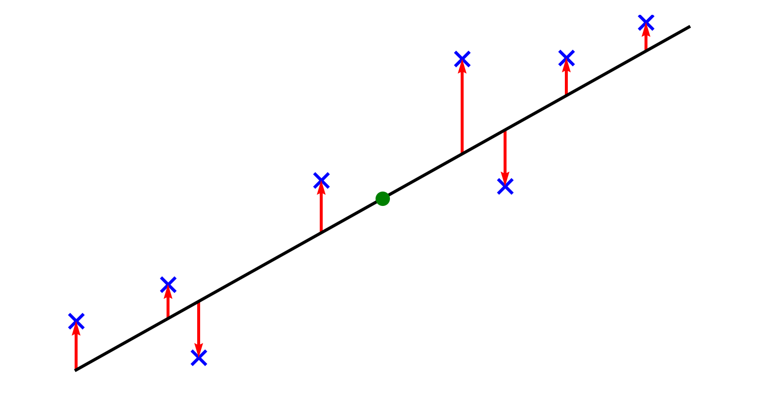
Figure 3: The mechanical analogy to a one-dimensional least-squares fit. The forces on the lever (red vectors) point from the lever positions $(x^{(i)},ax^{(i)})$ to the data points $(x^{(i)},y^{(i)})$. The support of the lever (the green point) is at the origin.

The total torque on the lever is given by

$$\vec{\tau}=\sum_{i=1}^{N}\vec{x}_{i}\times\vec{F}_{i}=\begin{pmatrix}0\\ 0\\ \sum_{i=1}^{N}x^{(i)}(y^{(i)}-ax^{(i)})\end{pmatrix}.$$ (74)

In mechanical equilibrium the lever will assume a position of zero torque, i.e.

$$\vec{\tau}=0\Leftrightarrow\sum_{i=1}^{N}x^{(i)}(y^{(i)}-ax^{(i)})=XY-aXX^{\mathrm{T}}=0.$$ (75)

The position, described by the lever’s slope $a$, in equilibrium is thus given by

$$a_{\mathrm{eq}}=(XX^{\mathrm{T}})^{-1}XY,$$ (76)

which coincides with best-fit solution $\hat{a}$ for the regression problem. The one-dimensional regression problem therefore behaves like a mechanical lever.

The power of the normal form in this example is the as-strong-as-possible decoupling of the involved quantities (the positions $x^{(j)}$) in the basis vectors of the space of outputs leaving $\hat{a}$ unchanged. Breaking the changes of $y$ down to changes of two outputs only allowed to formulate Eqs. (69) and (71) and led to the discovery of a simple mechanical analogy sharing some aspects of the mathematical problem.

The normal form can also give interesting insights into regression problems in higher dimensions. A mathematical problem related to linear regression is the estimation of gradients of functions by finite differences. Suppose the values $f(x)$ of a function at positions $x^{(i)}\in\mathbbm{R}^{2}$ are given and the goal is to estimate the gradient of $f$ at $x^{(0)}$. This can be done by means of a linear model

$$f(x)\approx f(x^{(0)})+\nabla f|_{x^{(0)}}^{\mathrm{T}}(x-x^{(0)}).$$ (77)

The best-fit estimate based on this model is given by Eq. (66), i.e.

$$\widehat{\nabla f}|_{x^{(0)}}=(XX^{\mathrm{T}})^{-1}XY,$$ (78)

where

$$X=(x^{(1)}-x^{(0)},\ldots,x^{(N)}-x^{(0)})\quad\text{and}\quad Y=\begin{pmatrix}f(x^{(1)})-f(x^{(0)})\\ \vdots\\ f(x^{(N)})-f(x^{(0)})\end{pmatrix}.$$ (79)

The directions in the space of values of $f$ which do not contribute to the estimate of $\nabla f$ can thus be parameterised by a basis of $\mathrm{ker}\,X$. It is interesting to apply this to finite difference schemes for estimating the gradient. For the forward differences

$$\frac{\partial f}{\partial x_{i}}|_{x^{(0)}}\approx\frac{1}{\delta}\left(f(x^{(0)}+\delta e_{i})-f(x^{(0)})\right),\quad i\in\{1,2\}$$ (80)

with $e_{i}$ denoting the unit vector in $i$-direction one has $x^{(1)}=x^{(0)}+\delta e_{1}$, $x^{(2)}=x^{(0)}+\delta e_{2}$. Thus,

$$X=\begin{pmatrix}\delta&0\\ 0&\delta\end{pmatrix}$$ (81)

and $\mathrm{ker}\,X=\{0\}$. This reflects the fact that all three function evaluations at $x^{(0)}$, $x^{(1)}$ and $x^{(2)}$ are needed to estimate the gradient using the forward difference. The same holds true for the backward difference too. A more interesting case is given by the finite difference scheme illustrated in Fig. 4.

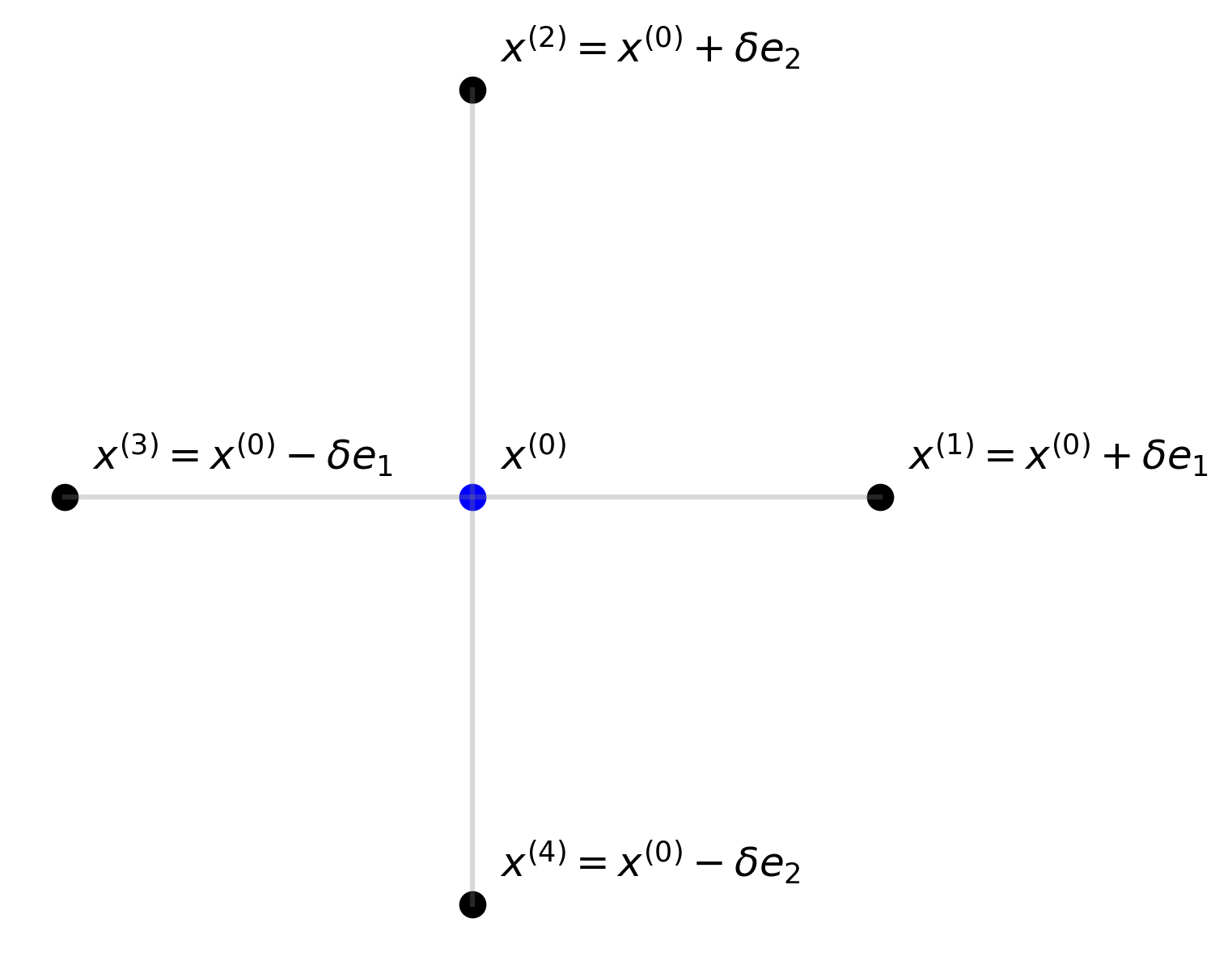
Figure 4: A finite difference scheme based on five function evaluations.

For this case

$$X=\delta\begin{pmatrix}[r]1&0&-1&0\\ 0&1&0&-1\end{pmatrix}$$ (82)

In normal form the basis of $\mathrm{ker}\,X$ is given by

$$(v_{1},v_{2})=\begin{pmatrix}1&0\\ 0&1\\ 1&0\\ 0&1\end{pmatrix}.$$ (83)

From this the two independent combinations of function evaluations not contributing to the gradient estimate are found to be

$$\begin{split}v_{1}^{\mathrm{T}}Y&=f(x^{(1)})-f(x^{(0)})+f(x^{(3)})-f(x^{(0)})\\ &=f(x^{(0)}+\delta e_{1})-2f(x^{(0)})+f(x^{(0)}-\delta e_{1}),\end{split}$$ (84a)

$$\begin{split}v_{2}^{\mathrm{T}}Y&=f(x^{(2)})-f(x^{(0)})+f(x^{(4)})-f(x^{(0)})\\ &=f(x^{(0)}+\delta e_{2})-2f(x^{(0)})+f(x^{(0)}-\delta e_{2}).\end{split}$$ (84b)

Since these linear combinations provide information going beyond the mere gradient information, they must contain information about higher order derivatives of $f$. Indeed, by Taylor expansion of $f$ one finds

$$\frac{1}{\delta^{2}}v_{1}^{\mathrm{T}}Y\xrightarrow[\delta\to 0]{}\frac{\partial^{2}f}{\partial x_{1}^{2}}|_{x^{(0)}},$$ (85a)

$$\frac{1}{\delta^{2}}v_{2}^{\mathrm{T}}Y\xrightarrow[\delta\to 0]{}\frac{\partial^{2}f}{\partial x_{2}^{2}}|_{x^{(0)}}.$$ (85b)

That is, the two basis vectors in normal form correspond to the two second order derivatives which can be estimated given the function evaluations of the scheme of Fig. 4.

4 Conclusions

The purpose of the normal form for bases proposed in this paper is to provide a technique to support the understanding of the structure of the problem in which the basis occurs. Sec. 3 illustrates the power of this technique in sample applications from different areas of physics and mathematics.

From the mathematical side, the most important properties required for the normal form are uniqueness and a high number of zero entries in the basis vectors. A widely used normal form for matrices which shares uniqueness and which also maps bases to bases is the reduced row echelon form (rref) which can be computed by Gauß-Jordan elimination—see textbooks on linear algebra. Given a basis of a finite-dimensional vector space as rows of a matrix, the rref fulfils

• All leading entries (leftmost non-zero entries) are one.

• Every column with a leading entry has zeros in all other places.

• The zero rows, if there are any, are below all non-zero rows.

This looks similar to the requirements on the normal form proposed in this paper. Indeed, for $A$ being a matrix of full column rank

$$A\mapsto\mathrm{rref}(A^{\mathrm{T}})^{\mathrm{T}},$$ (86)

which is the reduced column echelon form (rcef), provides a unique normal form for the basis of the vector space spanned by the columns of $A$. It, however, does not share the goal of having as many zero entries as possible and in general will not lead to the highest possible number of zero entries. As an illustration, take the basis of Eq. (35). Its rcef and its normal form are

$$\text{rcef: }\left(\begin{matrix}[r]1&0\\ 0&1\\ 0&-1\\ 1/2&1/2\\ -1/2&-1/2\end{matrix}\right),\quad\text{normal form: }\left(\begin{matrix}[r]1&1\\ -1&0\\ 1&0\\ 0&1/2\\ 0&-1/2\end{matrix}\right).$$ (87)

Though both forms are simple and structured, the rcef has less zero entries than the normal form. A case in which the rcef and the normal form strongly differ may be constructed as follows. Suppose $A$ and $B$ are two different, e.g. random, invertible $n\times n$-matrices and let the columns of the matrix

$$\begin{pmatrix}A\\ B\\ B\\ \vdots\\ B\end{pmatrix}$$ (88)

denote the basis of an $n$-dimensional vector space. Then the rcef will be given by

$$\begin{pmatrix}\mathbbm{1}\\ BA^{-1}\\ BA^{-1}\\ \vdots\\ BA^{-1}\end{pmatrix}$$ (89)

which will have many zero entries less than the normal form, which must have at least as many zeros as

$$\begin{pmatrix}AB^{-1}\\ \mathbbm{1}\\ \mathbbm{1}\\ \vdots\\ \mathbbm{1}\end{pmatrix}.$$ (90)

However, there is a tradeoff. The rcef is much easier to compute than the normal form. Therefore, in cases where the normal form is too expensive to compute, the rcef may be a good alternative.

To summarise, the normal form presented in this paper can be a powerful tool for unveiling the structure of problems involving bases of finite-dimensional vector spaces. An algorithm for its computation as well as an implementation for this algorithm are given in appendices A and B, respectively, and the readers are encouraged to use these to gain insight into the structure of their own problems.

Appendix A An algorithm for computing the normal form

The simplest algorithm for constructing the normal form is to generate all

$$\left(\begin{matrix}m\\ n-1\end{matrix}\right)=\frac{m!}{(n-1)!\,(m-n+1)!}$$ (91)

selections of $n-1$ rows of $A$, check whether the selected rows span an $(n-1)$-dimensional space and if so, construct the corresponding $\hat{s}$. Ordering the $\hat{s}$ then allows to construct the normal form. In the following this algorithm will be referred to as the standard algorithm. A possibility for such an algorithm is shown in the left part of Fig. 5. In practice, the normal form will be most interesting in cases where there are many more zero entries achievable in the basis vectors than the theoretical minimum of $n-1$. If the number of achievable zeros is close to the theoretical maximum $m-1$, an algorithm trying to construct $\hat{s}$ leading to $m-1,m-2,\ldots$ zeros in the basis vectors may be sufficiently faster in constructing the normal form. Namely, using this strategy, if after finishing the trial of all possibilities for $m-k$ zeros $n$ linearly independent $\hat{s}$ are found, the search can be stopped, since all not yet found $\hat{s}$ will have smaller $\theta(\hat{s})$. The number of selections to be tried is then

$$\sum_{j=1}^{k}\left(\begin{matrix}m\\ m-j\end{matrix}\right).$$ (92)

For small $k$ this search strategy will be advantageous. Since this algorithm searches “from the top” (highest possible number of zero entries first), in the following it will be referred to as the top-down algorithm. It is illustrated in the right part of Fig. 5.

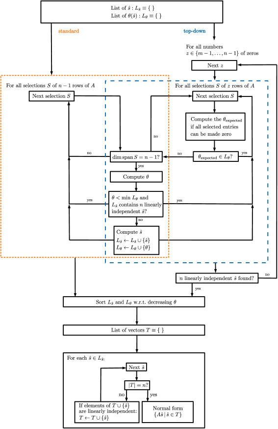
Figure 5: An algorithm for computing the normal form. Left (fine dashed): standard algorithm, right (dashed): top-down algorithm.

In appendix B a Python [10] implementation of both algorithms is provided.

Appendix B A Python implementation of the normal form

The following Python implementation allows to compute the normal form of real and complex matrices of full column rank. The function computing the normal form is defined in line 119 of the source code below, and an example for its use can be found following line 133.

Computation times for random matrices of sizes $20\times 10$ to $20\times 19$ with the standard algorithm range from less than a second to about 45 minutes on a typical personal computer. This is sufficient for the examples presented in this paper. For matrices which have many zero entries, the top-down algorithm will in general be much faster. As an illustration, consider the normal form of the basis of the example of Sec. 3.3 (see also Fig. 1). The basis is described by a $42\times 9$-matrix with twelve vanishing rows, effectively giving rise to a $30\times 9$ matrix. A very crude estimate for the running time of the standard algorithm in this case is

$$t_{\text{standard}}\sim\left(\begin{matrix}30\\ 8\end{matrix}\right)t_{\mathrm{SVD}},$$ (93)

where $t_{\mathrm{SVD}}$ is the typical time needed for one singular value decomposition in line 6 of the source code below. The resulting normal form has at most six non-zero entries in a column, see Eq. (52). Thus, for the top-down algorithm the according estimate is

$$t_{\text{top-down}}\sim\sum_{j=1}^{6}\left(\begin{matrix}30\\ 30-j\end{matrix}\right)t_{\mathrm{SVD}},$$ (94)

giving the estimate

$$\frac{t_{\text{standard}}}{t_{\text{top-down}}}\sim 7.6.$$ (95)

The measured times on a typical personal computer are $t_{\text{standard}}=478.1\,\text{s}$ and $t_{\text{top-down}}=111.3\,\text{s}$, i.e. $t_{\text{standard}}/t_{\text{top-down}}\approx 4.3$.

A rigorous analysis of the asymptotic complexities of the two presented algorithms, as well as a discussion of possible improvements is beyond the scope of this paper. The key message here shall be that for moderately sized matrices (up to $m,n\lesssim 15$) and even for larger examples like the $30\times 9$-matrix from Sec. 3.3, the presented algorithms and the provided implementation allow computation of the normal form in seconds to minutes.

The code below is licensed under the MIT license:

Copyright (c) 2023 Patrick Otto Ludl

Permission is hereby granted, free of charge, to any person obtaining a copy
of this software and associated documentation files (the "Software"), to deal
in the Software without restriction, including without limitation the rights
to use, copy, modify, merge, publish, distribute, sublicense, and/or sell
copies of the Software, and to permit persons to whom the Software is
furnished to do so, subject to the following conditions:

The above copyright notice and this permission notice shall be included in all
copies or substantial portions of the Software.

THE SOFTWARE IS PROVIDED "AS IS", WITHOUT WARRANTY OF ANY KIND, EXPRESS OR
IMPLIED, INCLUDING BUT NOT LIMITED TO THE WARRANTIES OF MERCHANTABILITY,
FITNESS FOR A PARTICULAR PURPOSE AND NONINFRINGEMENT. IN NO EVENT SHALL THE
AUTHORS OR COPYRIGHT HOLDERS BE LIABLE FOR ANY CLAIM, DAMAGES OR OTHER
LIABILITY, WHETHER IN AN ACTION OF CONTRACT, TORT OR OTHERWISE, ARISING FROM,
OUT OF OR IN CONNECTION WITH THE SOFTWARE OR THE USE OR OTHER DEALINGS IN THE
SOFTWARE.

⬇

1import numpy as np

2import itertools

3

4

5def compute_rank_and_kernel(A: np.ndarray, accuracy):

6 _, s, Vh = np.linalg.svd(A, full_matrices=True)

7 rank = np.sum(np.abs(s) > accuracy)

8 kernel = Vh[rank:, :].transpose()

9 return rank, kernel

10

11

12def are_linearly_independent(vectors: list, accuracy):

13 """vectors: List of 1-dim. numpy arrays"""

14 rank = np.linalg.matrix_rank(np.array(vectors).transpose(), accuracy)

15 return rank == len(vectors)

16

17

18def get_theta2_from_selection(selection: list):

19 """selection [list(0 or 1)]: list which indicates which rows of the matrix

20 are selected"""

21 theta2 = 0

22 for k in range(0, len(selection)):

23 theta2 += selection[k] * 2**k

24 return theta2

25

26

27class _NormalForm:

28 def __init__(self, A: np.ndarray, accuracy, top_down=False):

29 self.A = A

30 self.accuracy = accuracy

31 self.top_down = top_down

32 self.m = A.shape[0]

33 self.n = A.shape[1]

34 self.list_of_s_hat = []

35 self.list_of_theta = []

36 self.theta_min = 0

37 self.n_linearly_independent_s_hat_found = False

38

39 def _compute_theta(self, element_is_zero):

40 theta2 = get_theta2_from_selection(list(element_is_zero))

41 return 2**(self.m+sum(element_is_zero)) + theta2

42

43 def _update(self, theta, s, As, element_is_zero):

44 if theta not in self.list_of_theta:

45 index = np.where(np.logical_not(element_is_zero))[0][0]

46 s_hat = s / As[index]

47 self.list_of_theta = self.list_of_theta + [theta]

48 self.theta_min = min(self.list_of_theta)

49 self.list_of_s_hat = self.list_of_s_hat + [s_hat]

50 if not self.n_linearly_independent_s_hat_found:

51 if len(self.list_of_s_hat) >= self.n:

52 rank = np.linalg.matrix_rank(

53 np.concatenate(self.list_of_s_hat, axis=1),

54 self.accuracy)

55 self.n_linearly_independent_s_hat_found = (rank == self.n)

56

57 def _compute_transformation_matrix(self):

58 sorting_indices = list(reversed(sorted(range(len(self.list_of_theta)),

59 key=lambda k: self.list_of_theta[k])))

60 self.list_of_s_hat = [self.list_of_s_hat[i] for i in sorting_indices]

61 transformation_matrix = [self.list_of_s_hat[0]]

62 for k in range(1, len(self.list_of_s_hat)):

63 if len(transformation_matrix) == self.n:

64 break

65 if are_linearly_independent(transformation_matrix +

66 [self.list_of_s_hat[k]],

67 self.accuracy):

68 transformation_matrix = (transformation_matrix +

69 [self.list_of_s_hat[k]])

70 return np.concatenate(transformation_matrix, axis=1)

71

72 def _normalform(self):

73 for selection in itertools.combinations(range(0, self.m), self.n-1):

74 rank, s = compute_rank_and_kernel(self.A[selection, :],

75 self.accuracy)

76 if rank != self.n-1:

77 continue

78 As = (self.A@s).flatten()

79 element_is_zero = (np.abs(As) < self.accuracy)

80 theta = self._compute_theta(element_is_zero)

81 if (self.n_linearly_independent_s_hat_found

82 and theta < self.theta_min):

83 continue

84 self._update(theta, s, As, element_is_zero)

85

86 def _normalform_top_down(self):

87 for number_of_zeros in reversed(range(self.n-1, self.m)):

88 for selection in itertools.combinations(range(0, self.m),

89 number_of_zeros):

90 a = np.zeros(self.m).astype(np.int32)

91 a[list(selection)] = 1

92 theta2_expected = get_theta2_from_selection(list(a))

93 theta_expected = 2**(self.m+sum(a)) + theta2_expected

94 if theta_expected in self.list_of_theta:

95 continue

96 rank, s = compute_rank_and_kernel(self.A[selection, :],

97 self.accuracy)

98 if rank != self.n-1:

99 continue

100 As = (self.A@s).flatten()

101 element_is_zero = (np.abs(As) < self.accuracy)

102 theta = self._compute_theta(element_is_zero)

103 if (self.n_linearly_independent_s_hat_found and

104 theta < self.theta_min):

105 continue

106 self._update(theta, s, As, element_is_zero)

107 if self.n_linearly_independent_s_hat_found:

108 break

109

110 def compute(self):

111 if self.top_down:

112 self._normalform_top_down()

113 else:

114 self._normalform()

115 transformation_matrix = self._compute_transformation_matrix()

116 return self.A@transformation_matrix, transformation_matrix

117

118

119def normalform(A: np.ndarray, accuracy=1.0e-8, top_down=False):

120 rankA = np.linalg.matrix_rank(A, accuracy)

121 if rankA < A.shape[1]:

122 raise ValueError("Error: The normal form is only defined " +

123 "for matrices of full column rank. The matrix is " +

124 str(A.shape[0]) + " x " + str(A.shape[1]) +

125 " and its rank is " + str(rankA)+".")

126 # Check for zero rows in A. These can be neglected!

127 row_norms = np.linalg.norm(A, axis=1)

128 A_reduced = A[row_norms > accuracy, :]

129 _, transformation_matrix = _NormalForm(A_reduced, accuracy, top_down).compute()

130 return A@transformation_matrix, transformation_matrix

131

132

133if __name__ == "__main__":

134 A = np.array([[1, 1], [2, 2], [3, 3], [1, 2]])

135 print(A)

136

137 A_nf, _ = normalform(A)

138 A_nf_expected = np.array([[0, 1], [0, 2], [0, 3], [1, 0]])

139 assert np.linalg.norm(A_nf-A_nf_expected) < 1.0e-12

140

141 def chop(A: np.ndarray, limit=1.0e-15):

142 A_copy = A.copy()

143 A_copy[np.abs(A_copy) < limit] = 0

144 return A_copy

145

146 print(chop(A_nf))

References

- [1] J. W. Eaton et al., GNU Octave, www.octave.org.
- [2] E. Buckingham, On Physically Similar Systems; Illustrations of the Use of Dimensional Equations, Phys. Rev. 4 (1914), 345.
- [3] P. W. Bridgman, Dimensional Analysis (Yale University Press, New Haven, 1922).
- [4] C. R. Harris, K. J. Millman, S. J. van der Walt et al., Array programming with NumPy, Nature 585 (2020), 357–362.
- [5] S. Udrescu and M. Tegmark, AI Feynman: A physics-inspired method for symbolic regression, Science Advances 6 16 (2020), eaay2631. (arXiv:1905.11481v2 [physics.comp-ph])
- [6] E. Noether, Invariante Variationsprobleme, Nachrichten von der Gesellschaft der Wissenschaften zu Göttingen, Mathematisch-Physikalische Klasse 1918 (1918), 235-257.
- [7] E. H. Moore, On the reciprocal of the general algebraic matrix, Bulletin of the American Mathematical Society 26 (1920), 394–95.
- [8] A. Bjerhammar, Application of calculus of matrices to method of least squares; with special references to geodetic calculations, Trans. Roy. Inst. Tech. Stockholm 49 (1951).
- [9] R. Penrose, A generalized inverse for matrices, Proceedings of the Cambridge Philosophical Society 51 (3) (1955), 406–13.
- [10] G. van Rossum and The Python Software Foundation, Python, www.python.org.