Blind Video Quality Assessment at the Edge

Abstract

Owing to the proliferation of user-generated videos on the Internet, blind video quality assessment (BVQA) at the edge attracts growing attention. The usage of deep-learning-based methods is restricted to be applied at the edge due to their large model sizes and high computational complexity. In light of this, a novel lightweight BVQA method called GreenBVQA is proposed in this work. GreenBVQA features a small model size, low computational complexity, and high performance. Its processing pipeline includes: video data cropping, unsupervised representation generation, supervised feature selection, and mean-opinion-score (MOS) regression and ensembles. We conduct experimental evaluations on three BVQA datasets and show that GreenBVQA can offer state-of-the-art performance in PLCC and SROCC metrics while demanding significantly smaller model sizes and lower computational complexity. Thus, GreenBVQA is well-suited for edge devices.

1 Introduction

Objective video quality assessment methods are often classified into three categories: full-reference video quality assessment (FR-VQA), reduced-reference video quality assessment (RR-VQA), and no-reference video quality assessment (NR-VQA). NR-VQA is also known as blind video quality assessment (BVQA). FR-VQA methods assess video quality by measuring the difference between distorted videos and their reference videos. One well-known example is VMAF [1, 2]. RR-VQA [3] methods evaluate video quality by utilizing a part of information from reference videos, which offers greater flexibility than FR-VQA. Finally, BVQA is the only choice if there is no reference video available. With the rise of social media and the popularity of multi-party video conferencing, there has been an explosion of user-generated video content. A significant portion of the user-generated content lacks the availability of reference videos, necessitating the need for BVQA methods to automatically and efficiently evaluate perceptual video quality. Furthermore, the adoption of edge computing is on the rise, primarily attributable to its capacity to reduce latency, conserve network bandwidth, enhance privacy, and enable real-time data processing. In edge computing environments, BVQA plays a pivotal role in ensuring that video quality remains high while optimizing resources and responsiveness. Thus, BVQA attracts growing attention in recent years, as it addresses the pressing need of evaluating video quality in diverse contexts, spanning user-generated content and edge computing scenarios.

One straightforward BVQA solution is to build it upon blind image quality assessment (BIQA) methods. That is, the application of BIQA methods to a set of key frames of distorted videos individually. BIQA methods can be classified into three categories: natural scene statistic (NSS) based methods [4, 5, 6], codebook-based methods [7, 8] and deep-learning-based (DL-based) methods [9, 10]. However, directly applying BIQA followed by frame-score aggregation does not produce satisfactory outcomes because of the absence of temporal information. Thus, it is essential to incorporate temporal or spatio-temporal information. Other BVQA methods with handcrafted features [11, 12] were evaluated on synthetic-distortion datasets with simulated distortions such as transmission and compression. Recently, they were evaluated on authentic-distortion datasets as well as reported in [13, 14]. Their performance on authentic-distortion datasets is somehow limited. Authentic-distortion VQA datasets arise from the user-generated content (UGC) in the real-world environment. They contain complicated and mixed distortions with highly diverse contents, devices, and capture conditions.

Deep learning (DL) methods have been developed for BIQA and BVQA [10]. To further enhance performance and reduce distributional shifts [15], pre-trained models on large-scale image datasets, such as the ImageNet [16], are adopted in [17, 18]. However, it is expensive to adopt large pre-trained models on mobile or edge devices. Edge computing is a rapidly growing field in recent years due to the popularity of smartphones and Internet of Things (IoT). It involves processing and analyzing data near their source, typically at the “edge” of the network (rather than transmitting them to a centralized location such as a cloud data center). Given that a high volume of videos triggers heavy Internet traffic, video processing at the edge reduces the video transmission burden and saves the network bandwidth. The VQA task can enhance many video processing modules, such as video bitrate adaptation [19], video quality assurance [20], and video pre-processing [21]. The demand for high-quality videos is increasing on edge devices, while most user-generated contents lack reference videos, necessitating the use of BVQA methods. Furthermore, DL-based BVQA methods are expensive to deploy on edge devices due to their high computational complexity and large model sizes.

Therefore, a lightweight BVQA method is demanded at the edge. Based on the green learning principle [22, 23], a lightweight BIQA method, called GreenBIQA, was proposed in [24] recently. It is worth noting that GreenBIQA exhibits limited performance when applied to VQA datasets, primarily due to its lack of temporal information integration. Moreover, direct deployment of GreenBIQA in video quality evaluation is computationally expensive because of a huge difference in image and video data sizes. To address this void, we propose a lightweight BVQA method and call it GreenBVQA in this work. GreenBVQA features a smaller model size and lower computational complexity while achieving highly competitive performance against state-of-the-art DL methods. The processing pipeline of GreenBVQA contains four modules: 1) video data cropping, 2) unsupervised representation generation, 3) supervised feature selection, and 4) mean-opinion-score (MOS) regression and ensembles. The video data cropping operation in Module 1 is a pre-processing step. Then, we extract spatial, spatio-color, temporal, and spatio-temporal representations from cropped data in an unsupervised manner to obtain a rich set of representations at low complexity in Module 2 and select a subset of the most relevant features using the relevant feature test (RFT) [25] in Module 3. Finally, all selected features are concatenated and fed to a trained MOS regressor to predict multiple video quality scores and, then, an ensemble scheme is used to aggregate multiple regression scores into one ultimate score. conduct experimental evaluations on three VQA datasets and show that GreenBVQA can offer state-of-the-art performance in PLCC and SROCC metrics while demanding significantly small model sizes, short inference time, and low computational complexity.

There are three main contributions of this work.

• A novel lightweight BVQA method, named GreenBVQA, is proposed. Four different types of representation (i.e., spatial, spatio-color, temporal, and spatio-temporal representations) are considered jointly. Each type of representation is passed to the supervised feature selection module for dimension reduction. Then, all selected features are concatenated to form the final feature set.

• Experiments are conducted on three commonly used VQA datasets to demonstrate the advantages of the proposed GreenBVQA method. Our method outperforms all conventional BVQA methods in terms of MOS prediction accuracy. Its performance is highly competitive against DL-based methods while featuring a significantly smaller model size, shorter inference time, and lower computational complexity.

• A video-based edge computing system is presented to illustrate the role of GreenBVQA in facilitating various video processing tasks at the edge. The inherent characteristics of GreenBVQA, notably its lightweight model and low computational complexity, serve as a compelling evidence of its prospective utility in the realm of edge computing.

The rest of this paper is organized as follows. Related work is reviewed in Sec. 2. The proposed GreenBVQA is presented in Sec. 3. Experimental results are shown in Sec. 4. An edge computing system employing GreenBVQA is presented to demonstrate its potential real-world applications in Sec. 5. Finally, concluding remarks are given and future research directions are pointed out in Sec. 6.

2 Review of Related Work

Quite a few BVQA methods have been proposed in the last two decades. Existing work can be classified into conventional and DL-based methods two categories. They are first reviewed in Sec. 2.1 and sec. 2.2, respectively. Then, we examine previous work on video edge computing in Sec. 2.3

2.1 Conventional BVQA Method

Conventional BVQA methods extract quality-related features from input images using an ad hoc approach. Then, a regression model (e.g., Support Vector Regression (SVR) [26] or XGBoost [27]) is trained to predict the quality score using these handcrafted features. One family of methods is built upon the Natural Scene Statistics (NSS). NSS-based BIQA methods [5, 6] can be extended to NSS-based BVQA methods since videos are formed by multiple image frames. For example, V-BLIINDS [28] is an extension of a BIQA method by incorporating a temporal model with motion coherency. Spatio-temporal NSS can be derived from a joint spatio-temporal domain. For instance, the method in [29] conducts the 3D discrete cosine transform (DCT) and captures the spatio-temporal NSS of 3D-DCT coefficients. The spatio-temporal statistics of mean-subtracted and contrast-normalized (MSCN) coefficients of natural videos are investigated in [30], where an asymmetric generalized Gaussian distribution (AGGD) is adopted to model the statistics of both 3D-MSCN coefficients and bandpass filter coefficients of natural videos. Another family of BVQA methods, called codebook-based BVQA, is inspired by CORNIA [7], [31]. They first obtain frame-level quality scores using unsupervised frame-based feature extraction and supervised regression. Then, they adopt temporal pooling to derive the target video quality. A two-level feature extraction mechanism is employed by TLVQM [32], where high- and low-level features are extracted from the whole sequence and a subset of representative sequences, respectively.

2.2 DL-based BVQA Method

DL-based BVQA methods have been investigated recently. They offer state-of-the-art prediction performance. Inspired by MEON [33], V-MEON [34] provides an end-to-end learning framework by combining feature extraction and regression into a single stage. It adopts a two-step training strategy: one for codec classification and the other for quality score prediction. COME [35] adopts CNNs to extract spatial features and uses motion statistics as temporal features. Then, it exploits a multi-regression model, including two types of SVR, to predict the final score of videos. A mixed neural network is derived in [36]. It uses a 3D convolutional neural network (3D-CNN) and a Long-Short-Term Memory (LSTM) network as the feature extractor and the quality predictor, respectively. Following the VSFA method [37], MDTVSFA [17] adopts an unified BVQA framework with a mixed-dataset training strategy to achieve better prediction performance against authentic-distortion video datasets. PVQ [38] adopts a local-to-global region-based BVQA architecture, which is trained with different kinds of patches. Also, a large authentic-distortion video dataset is built and reported in [38]. QSA-VQM [39] uses two CNNs to extract quality attributes and semantic content of each video frame, respectively, and one Recurrent Neural Network (RNN) to estimate the quality score of the whole video by incorporating temporal information. To address the diverse range of natural temporal and spatial distortions commonly observed in user-generated-content datasets, CNN-TLVQM [40] integrates spatial features obtained from a CNN model and handcrafted statistical temporal features obtained via TLVQM. The CNN model was originally trained for image quality assessment using a transfer learning technique.

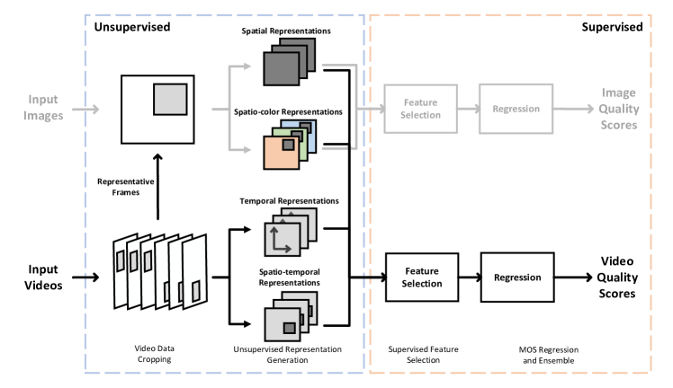
Figure 1: The system diagram of the proposed GreenBVQA method.

2.3 Video Quality Assessment at the Edge

Machine learning models have been extensively deployed on edge devices [41]. Several video analytics tasks are implemented in the edge computing platform [42]. Besides prediction accuracy, important metrics to be considered at the edge include latency, computational complexity, memory size, etc. The remarkable success achieved by DL in various domains, such as computer vision and natural language processing, has inspired the application of DL to edge devices (say, smartphones and IoT sensors) [43]. They often generate a significant amount of data that demand local processing due to the high data communication cost. Edge computing has emerged in video analytics in recent years. One objective is to optimize the tradeoff between accuracy and cost [42]. For example, VideoEdge [44] is an edge-based video analysis tool that is implemented in a distributed cloud-edge architecture, comprising edge nodes and the cloud.

Given heavy video traffics on mobile or edge networks, there is a growing demand for higher transmission rates and lower network latency. In order to tackle these challenges, adaptive bitrate (ABR) technologies [19, 45] are commonly used in video distribution. The ABR scheme consists of two main components. First, the video is encoded into multiple streaming versions with different bit rates. Second, each streaming version is segmented into multiple segments based on the terminal capabilities and network conditions. Consequently, the most suitable streaming version is dynamically provided to the user. The advantage of ABR lies in its ability to reduce the occurrence of choppy videos while enhancing user’s quality of experience (QoE).

To enhance QoE at the edge, one essential technology is the automatic measure of user’s perceptual video quality. As stated in [46], a better understanding of human perceptual experience and behavior is the most dominating factor in improving the performance of ABR algorithms. Since reference videos are not available on edge devices, BVQA methods become the only option. State-of-the-art BVQA methods rely on large pre-trained models and exhibit high computational complexity, making them impractical for deployment on edge devices. Lightweight BVQA methods are in urgent need to address this void. Along this line, Mirko et al. [47] propose an efficient BVQA method with two lightweight pre-trained MobileNets [48] with certain limitations, such as degraded prediction accuracy.

3 GreenBVQA Method

The system diagram of the proposed GreenBVQA method is shown in Fig. 1. It has a modularized system consisting of four modules: 1) video data cropping, 2) unsupervised representation generation, 3) supervised feature selection, and 4) MOS regression and ensemble. We will elaborate the operations in each module below.

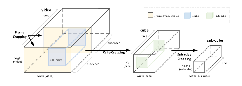
Figure 2: The video data cropping module of GreenBVQA.

3.1 Video Data Cropping

GreenBVQA adopts a hierarchical data cropping approach as illustrated in Fig. 2. This serves as a pre-processing step for later modules. Upon receiving an input video clip, we first split it into multiple sub-videos in the time domain. For instance, a ten-second video can be partitioned into ten non-overlapping sub-videos, each of one-second duration. The sub-video serves as the basic unit for future processing. Given a sub-video, we consider the following three cropping schemes.

1. Frame Cropping
   One representative frame is selected from each sub-video. It can be the first frame, an I-frame, or an arbitrary frame. Here, we aim to get spatial-domain information. For example, several sub-images can be cropped from a representative frame. Both spatial and spatio-color representations will be computed from each sub-image to be discussed in the next subsection.

2. Cube Cropping
   We collect co-located sub-images from all frames in one sub-video as shown in Fig. 2. This process is referred to as “cube cropping" since it contains both spatial and temporal information. The purpose of cube cropping is to reduce the amount of data to be processed in the later modules. This is needed as the data size of videos is substantially larger than that of images.

3. Sub-cube Cropping
   We crop out a sub-cube from a cube that has a shorter length in the time domain and a smaller size in the spatial domain (see Fig. 2). It is used to extract spatio-temporal representations. The rationale for sub-cube cropping is akin to that of cube cropping - reducing the amount of data to be processed later.

The rationale behind is that, considering the substantial video data amount, it is impractical to process the entirety of the data. Instead, hierarchical data cropping is employed as a means to gradually curtail the volume of data processing, while ensuring that excessive data is not discarded abruptly at any one stage of the cropping process.

3.2 Unsupervised Representation Generation

We consider the following four representations in GreenBVQA.

1. Spatial representations. They are extracted from the Y channel of sub-images cropped from representative frames.

2. Spatio-Color representations. They are extracted from cubes of size $(H\times W)\times C$, where $H$ and $W$ are the height and width of sub-images and $C=3$ is the number of color channels, respectively.

3. Temporal representations. They are the concatenation of statistical temporal information of cubes.

4. Spatio-Temporal representations. They are extracted from sub-cubes of size $(H\times W)\times T$, where $H$ and $W$ are the height and width of sub-images and $T$ is the length of sub-cubes in the time domain, respectively.

GreenBVQA employs all four types of representations collectively to predict perceptual video quality scores. On the other hand, spatial and spatio-color representations can be utilized to predict the quality scores of individual images or sub-images.

Table 1: The selected hyper-parameters for spatial representation generation in our experiments, where the transform dimensions are denoted by {$(H\times W)\text{, }C$} for spatial and channel dimensions, the stride parameter is denoted as {Spatial Stride²}, and L, M, and H represent low-frequency, mid-frequency, and high-frequency representations, respectively.

Layer	Spatial			Output Size
Input	$320\times 320$			$320\times 320$
DCT	$(8\times 8),1$			$(40\times 40),64$
Split	Low-freq (L)		High-freq (H)	L: $(40\times 40),1$ H: $(40\times 40),63$
Hop1	$(4\times 4),1$ stride 22		-	L: $(19\times 19),16$ H: $(40\times 40),63$
Split	Low-freq (L)	Mid-freq (M)	High-freq (H)	L: $(19\times 19),3$ M: $(19\times 19),13$ H: $(40\times 40),63$
Pooling	$(1\times 1),3$	$(2\times 2),13$	$(4\times 4),63$	L: $(19\times 19),3$ M: $(9\times 9),13$ H: $(10\times 10),63$
Hop2	$(3\times 3),3$ stride 22	-	-	L: $(9\times 9),27$ M: $(19\times 19),13$ H: $(10\times 10),63$

Table 2: The selected hyper-parameters for spatial-color representations generation, where the transform dimensions are denoted by {$(H\times W)\times T\text{, }C$} for spatial, color, and channel dimensions and $L$ and $H$ represent low-frequency and high-frequency representations, respectively.

Layer	Spatio-color		Output Size
Input	$(320\times 320)\times 3$		$(320\times 320)\times 3$
Pooling	$(2\times 2)\times 1$		$(160\times 160)\times 3$
Hop1	$(4\times 4)\times 3$		$(40\times 40)\times 1,48$
Split	Low-freq (L)	High-freq (H)	L: $(40\times 40)\times 1,3$ H: $(40\times 40)\times 1,45$
Pooling	-	$(2\times 2)\times 1,45$	L: $(40\times 40)\times 1,3$ H: $(20\times 20)\times 1,45$
Hop2	$(4\times 4)\times 1,1$	-	L: $(10\times 10)\times 1,48$ H: $(20\times 20)\times 1,45$

Table 3: The selected hyper-parameters for spatial-temporal representations generation, where the transform dimensions are denoted by {$(H\times W)\times T\text{, }C$} for spatial, temporal, and channel dimensions and $L$ and $H$ represent low-frequency and high-frequency representations, respectively.

Layer	Spatio-temporal		Output Size
Input	$(96\times 96)\times 15$		$(96\times 96)\times 15$
Pooling	-		$(96\times 96)\times 15$
Hop1	$(8\times 8)\times 3$		$(12\times 12)\times 5,192$
Split	Low-freq (L)	High-freq (H)	L: $(12\times 12)\times 5,4$ H: $(12\times 12)\times 5,188$
Pooling	-	$(2\times 2)\times 1,188$	L: $(12\times 12)\times 5,4$ H: $(6\times 6)\times 5,188$
Hop2	$(2\times 2)\times 5,4$	-	L: $(6\times 6)\times 1,80$ H: $(6\times 6)\times 5,188$

3.2.1 Spatial Representations

As discussed in deriving the spatial representation for GreenBIQA [49], a three-layer structure is adopted to extract local and global spatial representations from the sub-images. This is summarized in Table 1 and depicted in Fig. 3. Input sub-images are partitioned into non-overlapping blocks of size $8\times 8$, and the Discrete Cosine Transform (DCT) coefficients are computed through the block DCT transform. These coefficients, consisting of one DC coefficient and 63 AC coefficients (AC1-AC63), are organized into 64 channels. The DC coefficients exhibit correlations among spatially adjacent blocks, which are further processed by using the Saab transform [50]. The Saab transform computes the patch mean, referred to as the DC component, using a constant-element kernel. Principal Component Analysis (PCA) is then applied to the mean-removed patches to derive data-driven kernels, known as AC kernels. The AC kernels are applied to each patch, resulting in AC coefficients of the Saab transform. To decorrelate the DC coefficients, a two-stage process, namely Hop1 and Hop2, is employed. The coefficients obtained from each channel, either with or without down-sampling at different Hops and the DCT layer, are utilized to calculate standard deviations, PCA coefficients, or are left unchanged. According to the spectral frequency in DCT and Saab domain, the coefficients from Hop2, Hop1, and the DCT layer are denoted as low-frequency, mid-frequency, and high-frequency representations, respectively. Low- and mid-frequency representations contain global information from large receptive fields, while high-frequency representations contain information of details from a small receptive field. Then, all representations are concatenated to form spatial representations.

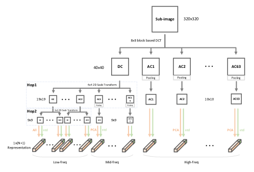
Figure 3: The block diagram of unsupervised spatial representation generation.

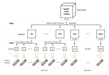
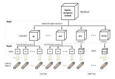
(a) Generation of spatiao-color representations	(b) Generation of spatio-temporal representations

Figure 4: The block diagram of unsupervised spatio-color and spatio-temporal representations generation.

3.2.2 Spatio-Color Representations

The representations for spatio-color cubes are derived using 3D Saab and PCA methods. The hyper-parameters are given in Table 2, and the data processing block diagram is depicted in Fig. 4 (a). A spatio-color cuboid has dimensions of $H\times W\times C$, where $H$ and $W$ represent the height and width of the sub-image respectively, and $C=3$ denotes the number of color channels. It is fed to a two-hop structure. In Hop1, it is divided into non-overlapping cuboids of size $4\times 4\times 3$, and the 3D Saab transform is applied individually, resulting in one DC channel and 47 AC channels (AC1-AC47). Each channel has a spatial dimension of $40\times 40$. Since the DC, AC1, and AC2 coefficients exhibit high spatial correlation, in Hop2, a 2D Saab transform is used to decompose these channels of size $40\times 40$ into non-overlapping blocks of size $4\times 4$. For the other 45 AC coefficients obtained from Hop1, their absolute values are taken and a $2\times 2$ max pooling operation is performed, yielding 45 channels with a spatial dimension of $20\times 20$. In total, we obtain 93 channels, comprising 48 low-frequency channels from Hop2 and 45 high-frequency channels from Hop1, with spatial size of $10\times 10$ and $20\times 20$, respectively. The coefficients obtained from each channel are utilized to calculate standard deviations and PCA coefficients. These computed coefficients are then concatenated to form spatio-color representations.

Table 4: Summary of 14-D raw temporal representations.

Index	Computation Procedure
$f_{1}-f_{2}$	Compute the mean of x-mvs and y-mvs
$f_{3}-f_{4}$	Compute the standard deviation of x-mvs and y-mvs
$f_{5}-f_{6}$	Compute the ratio of significant x-mvs and y-mvs
$f_{7}-f_{8}$	Collect the maximum of x-mvs and y-mvs
$f_{9}-f_{10}$	Collect the minimum of x-mvs and y-mvs
$f_{11}$	Compute the mean of magnitude of mvs
$f_{12}$	Compute the standard deviation of magnitude of mvs
$f_{13}$	Compute the ratio of significant magnitude of mvs
$f_{14}$	Collect the maximum of magnitude of mvs

3.2.3 Temporal Representation

The spatial and spatio-color representations are extracted from the sub-images on representative frames. Both of them represent the information within individual frames while disregarding the temporal information across frames. Here, a temporal representation generation is proposed to capture the temporal information from motion vectors (mvs).

Consider a cube of dimensions $H\times W\times T$, where $H$ and $W$ represent the height and width of sub-images, respectively, and $T$ is the number of frames in the time domain. For each $H\times W$ sub-image within a cube, motion vectors of small blocks are computed (or collected from compressed video streaming). They are denoted as ${\bf V}=((x_{1},y_{1})\cdots,(x_{n},y_{n}))^{T}$, where $(x_{n},y_{n})$ represents the motion vector of the $n^{th}$ block. Specifically, $x_{n}$ and $y_{n}$ are the horizontal magnitude and vertical magnitude of the motion vector and are named x-mv and y-mv, respectively. The magnitude of the motion vector can be computed by $\sqrt{x_{n}^{2}+y_{n}^{2}}$.

The motion representation of a cube is computed based on its motion vectors. This statistical analysis yields a 14-D temporal representation of each sub-image as shown in Table 4. They are arranged in chronological order to form raw temporal representations. Furthermore, PCA is applied to them to derive spectral temporal representations. Finally, the raw and spectral temporal representations are concatenated to form the final temporal representations.

3.2.4 Spatio-Temporal Representation

Both spatial representations from sub-images of representative frames and temporal representations from cubes are extracted individually from a single domain. It is also important to consider the correlation between spatial information and temporal information in subjective score prediction, as subjective assessments often take both aspects into account when providing scores. To extract spatio-temporal features from both spatial and temporal domains, a two-hop architecture is adopted, where the 3D Saab transform is conducted as depicted in Fig. 4 (b). The hyper-parameters are summarized in Table 3

The dimension of the spatio-temporal cube, which is the same as sub-cubes in Fig. 2, is $H\times W\times T$, where $H$, $W$ and $T$ represent the height, width, and the frame number of the sub-cube, respectively. These sub-cubes are fed into a two-hop architecture, where the first and the second hops are used to capture local and global representations, respectively. The procedure used to generate spatio-temporal representation is similar to that for the spatio-color representation generation, except the 3D channel-wise Saab transform is applied in both hops. In Hop 1, we split the input sub-cubes into non-overlapping 3-D cuboids of size $8\times 8\times 3$. They are converted to one-dimensional vectors for Saab coefficient computation, leading to one DC channel and 191 AC channels, denoted by AC1-AC191. The size of each channel is $12\times 12\times 5$. The coefficients in DC and low-frequency AC (e.g., AC1-AC3) channels are spatially and temporally correlated because the adjacent $8\times 8\times 3$ cuboids are strongly correlated. Therefore, another 3-D Saab transform is applied in Hop 2 to decorrelate the DC and low-frequency AC channels from Hop 1. Similarly, we split these channels into several non-overlapping 3D cuboids of size $2\times 2\times 5$. Coefficients in each cuboid are flattened into a 20-D vector denoted by ${\bf y}=(y_{1},\cdots,y_{20})^{T}$, and their Saab coefficients are computed. The DC coefficients in Hop 2 are computed by the mean of the 20-D vector, $\bar{y}=(\sum_{i=1}^{20}y_{i})/20$. The remaining 19 AC coefficients, denoted by AC1 to AC19, are generated by the principle component analysis (PCA) on the mean-removed 20-D vector.

To lower the number of coefficients that need to be processed, blocks in Hop 1 are downsampled to cuboids of size $6\times 6\times 5$ by using $2\times 2$ max pooling in the spatial domain. Given low-frequency channels of size $6\times 6\times 1$ from Hop 2 and downsampled $6\times 6\times 5$ high-frequency channels from Hop 1, we generate two sets of representations as follows.

• The coefficients in each channel are first flattened to 1-D vectors. Next, we conduct PCA and select the first $N$ PCA coefficients of each channel to form the spectral features.

• We compute the standard deviation of coefficients from the same channel across the spatio-temporal domain.

Finally, we concatenate the two sets of representations to form the spatio-temporal representations.

3.3 Supervised Feature Selection

The number of unsupervised representations is large. To reduce the dimension of unsupervised representations, we select quality-relevant features from the 4 sets of representations obtained in the unsupervised representation generation part, by adopting the relevant feature test (RFT) [25]. RFT enables the calculation of independent losses for each representation, with lower loss values indicating superior representations. The RFT procedure involves splitting the dynamic range of a representation into two sub-intervals using a set of partition points. For a given partition, the means of the training samples in the left and right regions are computed as representative values, and their respective mean-squared errors (MSE) are calculated. By combining the MSE values of both regions, a weighted MSE for the partition is obtained. The search for the minimum weighted MSE across the set of partition points determines the cost function for the representation. It is important to note that RFT is a supervised feature selection algorithm as it utilizes the labels of the training samples.

We computed the RFT results for spatial, spatio-color, temporal, and spatio-temproal representations individually. Fig. 5 illustrates the sorting of representation indices based on their MSE values, with separate curves. The order of representations based on their MSE values implies that dimensions of representation with lower MSE are more likely to possess discriminative characteristics, thus signifying their potential value as features. In order to effectively collect features with discriminative attributes while concurrently reducing the dimensionality of the representations, an efficient strategy involves the selection of the top-ranked representation indices derived from the RFT results. The identification of relevant representation subsets is facilitated by pinpointing positions near the elbow points on each curve. Consequently, considering the existence of four distinct types of unsupervised representations, a subset comprising the highest-ranked indices for each representation type is chosen. The selected indices are then concatenated to constitute a set of supervised quality-relevant features for each cube. The dimensions of the unsupervised representations and the supervised features chosen in this manner are shown in Table 5, with particular focus on their application to the KoNViD-1k dataset as delineated in [51].

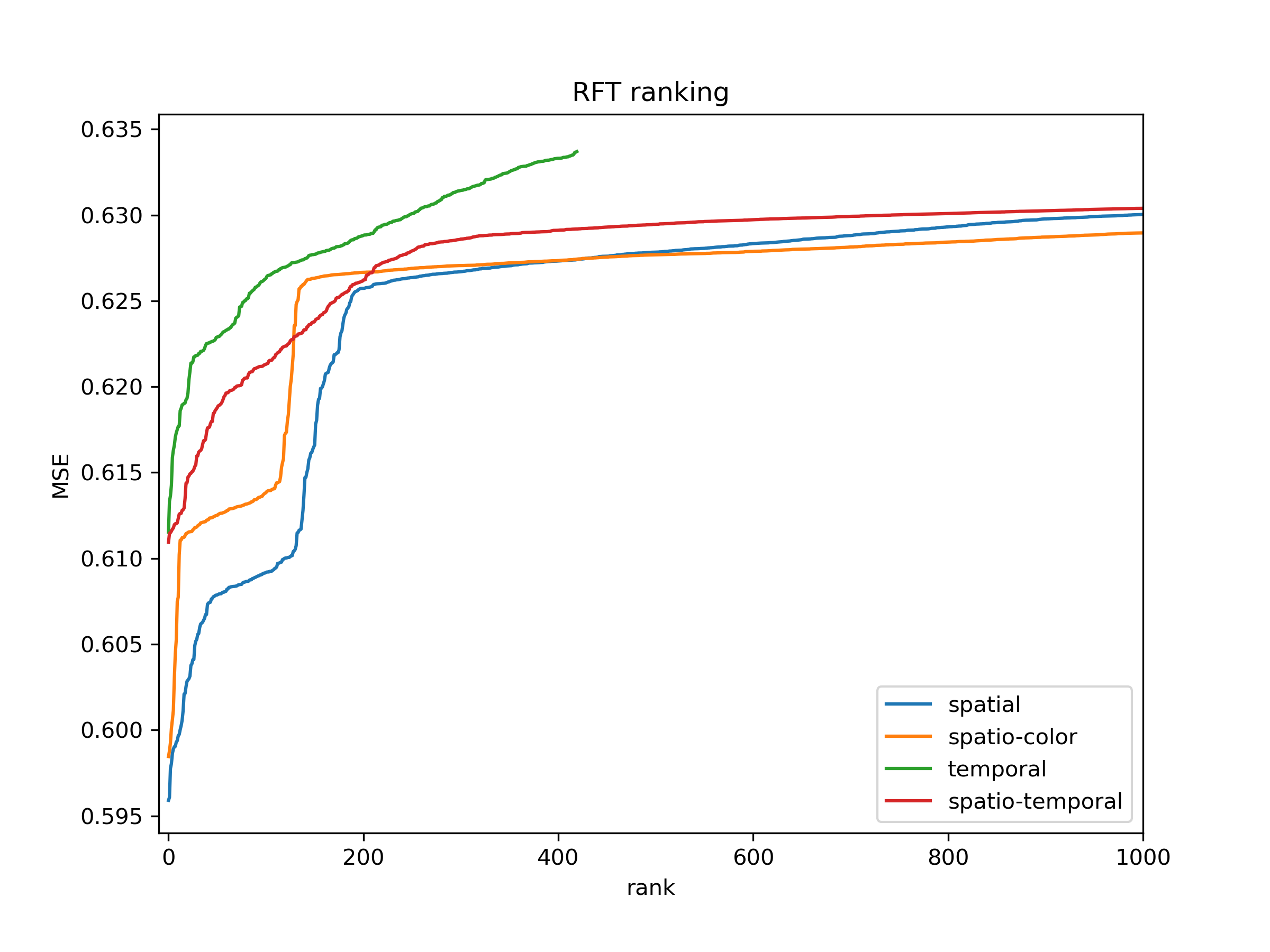
Figure 5: RFT results of spatial, spatio-color, temporal, and spatio-temporal representations.

Table 5: Dimensions of unsupervised representation and selected supervised features on KoNViD-1k dataset.

	Representation	Feature
	Dimension	Dimension
Spatio	6,637	220
Spatio-color	6,793	200
Temporal	420	140
Spatio-temporal	8,878	240
Sum	22,728	800

3.4 MOS Regression and Ensembles

Once the quality-relevant features are selected, we employ the XGBoost [27] regressor as the quality score prediction model that maps $d$-dimensional quality-relevant features to a single quality score. After the regressor’s prediction, each cube is assigned a predicted score. The scores of cubes belonging to the same sub-video are then ensembled using a median filter, resulting in the score of the sub-video, which predict the Mean Opinion Score (MOS) of a short interval of frames from the input video. To obtain the final MOS for the entire input video, a mean filter is applied to aggregate the scores from all sub-videos belonging to the same input video.

Table 6: Statistics of three VQA datasets.

Dataset	Ref.	Scenes.	Resolution	Time Duration	MOS range	Environment
CVD2014 [52]	234	5	480p, 720p	10-25s	[-6.50, 93.38]	In-lab
KoNViD-1k [51]	1,200	1,200	540p	8s	[1.22, 4.64]	Crowdsourced
LIVE-VQC [53]	585	585	240p-1080p	10s	[6.2237, 94.2865]	Crowdsourced

4 Experiments

4.1 Experiments Setup

We discuss VQA datasets, performance benchmarking methods, evaluation metrics, and some implementation details below.

4.1.1 Datasets

We evaluate GreenBVQA on three VQA datasets: CVD2014 [52], KoNViD-1k [51], and LIVE-VQC [53]. Their statistics are summarized in Table 6. CVD2014 is captured in a controlled laboratory environment. Thus, it is also called the lab-generated dataset. It comprises 234 video sequences of resolution $640\times 480$ or $1280\times 720$. They are acquired with 78 cameras ranging from low-quality mobile phones to high-quality digital single-lens reflex cameras. Each video displays one of five scenes with distortions associated with the video acquisition process. KoNViD-1k and LIVE-VQC are authentic-distortion datasets, also known as user-generated content (UGC) datasets. KoNViD-1k comprises 1200 video sequences, each of which lasts for 8 seconds with a fixed resolution. LIVE-VQC consists of a collection of video sequences of a fixed duration in multiple resolutions. Both of them contain diverse content and a wide range of distortions.

4.1.2 Benchmarking Methods

We compare the performance of GreenBVQA with eleven benchmarking methods in Table 7. These methods can be classified into three categories.

• Three conventional BIQA methods: NIQE [4], BRISQUE [6], and CORNIA [7]. They are applied to frames of distorted videos. Then, the predicted scores are ensembled to yield the ultimate BVQA score.

• Three conventional BVQA methods without neural networks: V-BLIINDS [13], TLVQM [32], and VIDEVAL [54].

• Five state-of-the-art DL-based methods with pre-trained models: VSFA [37], RAPIQUE [18], QSA-VQM [39], Mirko et al. [47], and CNN-TLVQM [40]. They are also called advanced DL methods.

4.1.3 Evaluation Metrics

The MOS prediction performance is measured by two well-known metrics: the Pearson Linear Correlation Coefficient (PLCC) and the Spearman Rank Order Correlation Coefficient (SROCC). PLCC is employed to assess the linear correlation between the predicted scores and the subjective quality scores. It is defined as

$$\textit{PLCC}=\frac{\sum_{i}(p_{i}-p_{m})(\hat{p_{i}}-\hat{p_{m}})}{\sqrt{\sum_{i}(p_{i}-p_{m})^{2}}\sqrt{\sum_{i}(\hat{p_{i}}-\hat{p_{m}})^{2}}},$$ (1)

where $p_{i}$ and $\hat{p_{i}}$ denote the predicted score and the corresponding subjective quality score, respectively, for a test video sample. Additionally, $p_{m}$ and $\hat{p_{m}}$ represent the means of the predicted scores and subjective quality scores, respectively. SROCC is used to measure the monotonic relationship between the predicted scores and the subjective quality scores, considering the relative ranking of the samples. It is defined as

$$\textit{SROCC}=1-\frac{6\sum_{i=1}^{L}(m_{i}-n_{i})^{2}}{L(L^{2}-1)},$$ (2)

where $m_{i}$ and $n_{i}$ represent the ranks of the predicted score $p_{i}$ and the corresponding subjective quality score $\hat{p_{i}}$, respectively, within their respective sets of scores. The variable $L$ represents the total sample number.

4.1.4 Implementation Details

Video Data Cropping. Each sub-video has a length of 30 frames. To derive a representative frame for each of these sub-videos, a straightforward selection process designates the first frame of each sub-video. From each such representative frame, a set of six sub-images, each possessing dimensions of $320\times 320$ pixels, is randomly cropped. Consequently, each cube consists of $(320\times 320)\times 30$ pixels, and a single sub-video harboring a complement of six such cubes. Specifically, in the context of generating spatio-temporal representations, sub-cubes are derived from these cubes. These sub-cubes are intentionally configured to assume dimensions of $(96\times 96)\times 15$. The dimensions $(96\times 96)$ denote the central region cropped from the sub-images, while the sub-cubes’ temporal component is constructed by collecting frames at every two-frame intervals within their corresponding cubes. Notably, the selection process ensures that only a solitary sub-cube is cropped from each cube.

Unsupervised Representation Generation. For spatial representation generation, the $8\times 8$ DCT transform and the $4\times 4$ Saab transform are used to generate spatial representations of 6,637 dimensions, as shown in Table 1. Similarly, in accordance with the structure outlined in Table 2 and Table 3, the dimensions of spatio-temporal and spatio-color representations are 8,878 and 6,793, respectively. Furthermore, it is noteworthy that the generation of temporal representations involves the computation of 14-dimensional representations, as shown in Table 4, for each individual frame within a cube. Consequently, the cumulative temporal representation for each cube aggregates to a dimensionality of 420.

Supervised Feature Selection. Following the application of RFT to each type of representation generated from the KoNViD-1k dataset, independently, the resulting selected features exhibit dimensions of 220 for spatial features, 200 for spatio-color features, 140 for temporal features, and 240 for spatio-temporal features. It is important to note that the dimensions of the selected features may vary across different datasets, as the distribution of data and content can differ among various datasets.

MOS Regression and Ensembles. The XGBoost regressor is used to train and predict the MOS score of each cube. The max depth of each tree is 5 and the subsampling rate is 0.6. The maximum number of trees is 2,000 with early termination. Given the score of each cube, a median filter is used to obtain the score of each sub-video. Next, we take the average of all sub-videos’ scores to obtain the final score of the input video.

Performance Evaluation. To ensure reliable evaluation, we partition a VQA dataset into two disjoint sets: the training set (80%) and the testing set (20%). We set 10% aside in the training set for validation purpose. We conduct experiments in 10 runs and report the median values of PLCC and SROCC.

Table 7: Comparison of the PLCC and SROCC performance of 10 benchmarking methods against three VQA datasets.

	CVD2014		LIVE-VQC		KoNViD-1k		Average
Model	SROCC$\uparrow$	PLCC$\uparrow$	SROCC$\uparrow$	PLCC$\uparrow$	SROCC$\uparrow$	PLCC$\uparrow$	SROCC$\uparrow$	PLCC$\uparrow$
NIQE[4]	0.475	0.607	0.593	0.631	0.539	0.551	0.535	0.596
BRISQUE[6]	0.790	0.804	0.593	0.624	0.649	0.651	0.677	0.654
CORNIA[7]	0.627	0.663	0.681	0.723	0.735	0.735	0.681	0.707
V-BLIINDS[13]	0.795	0.806	0.681	0.699	0.706	0.701	0.727	0.735
TLVQM[32]	0.802	0.823	0.783	0.785	0.763	0.765	0.782	0.791
VIDEVAL[54]	0.814	0.832	0.744	0.748	0.770	0.771	0.776	0.783
VSFA[37]	0.850	0.859	0.717	0.770	0.794	0.798	0.787	0.809
RAPIQUE[18]	0.807	0.823	0.741	0.761	0.788	0.805	0.778	0.796
QSA-VQM [39]	0.850	0.859	0.742	0.778	0.801	0.802	0.797	0.813
Mirko et al.[47]	0.834	0.848	0.742	0.780	0.772	0.784	0.782	0.804
CNN-TLVQM [40]	0.852	0.868	0.811	0.828	0.814	0.817	0.825	0.837
GreenBVQA(Ours)	0.835	0.854	0.785	0.789	0.776	0.779	0.798	0.807

4.2 Performance Comparison

4.2.1 Same-Domain Training Scenario

We compare the PLCC and SROCC performance of GreenBVQA with that of the other eleven benchmarking methods in Table 7. GreenBVQA outperforms all three conventional BIQA methods (i.e., NIQE, BRISQUE, and CORNIA) and all three conventional BVQA methods (i.e., V-BLIINDS, TLVVQM, and VIDEVAL) by a substantial margin in all three datasets. This shows the effectiveness of GreenBVQA in extracting quality-relevant features to cover diverse distortions and content variations. GreenBVQA is also competitive with the five DL-based BVQA methods. Specifically, GreenBVQA achieves the second-best performance for the LIVE-VQC dataset. It also ranks second in the average performance of SROCC across all three datasets.

As to the five DL-based BVQA methods, the performance of GreenBVQA is comparable with that of QSA-VQM. However, there exists a performance gap between GreenBVQA and CNN-TLVQM, which is a state-of-the-art DL-based method employing pre-trained models. The VQA datasets, particularly user-generated content datasets, pose significant challenges due to non-uniform distortions across videos and a wide variety of content without duplication. Pre-trained models, trained on large external datasets, have an advantage in extracting features for non-uniform distortions and unseen content. Nonetheless, these advanced DL-based methods come with significantly larger model sizes and inference complexity as analyzed in Sec. 4.3.

4.2.2 Cross-Domain Training Scenario

To evaluate the generalizability of BVQA methods, we investigate the setting where training and testing data come from different datasets. Here, we focus on the two UGC datasets (i.e., KoNViD-1k and LIVE-VQC) due to their practical significance. Two settings are considered: I) trained with KoNViD-1k and tested on LIVE-VQC, and II) trained with LIVE-VQC and tested on KoNViD-1k. We compare the SROCC performance of GreenBVQA and five benchmarking methods under these two settings in Table 8. The five benchmarking methods include two conventional BVQA methods (TLVQM, and VIDEVAL) and three DL-base BVQA methods (VSFA, QSA-VQM, and Mirko et al.).

We see a clear performance drop for all methods in the cross-domain condition by comparing Tables 7 and 8. We argue that setting II provides a more suitable scenario to demonstrate the robustness (or generalizability) of a learning model. This is because KoNViD-1k has a larger video number and scene number as shown in Table 6. Thus, we compare the performance gaps in Table 8 under Setting II with those in the KoNViD-1k/SROCC column in Table 7. The gaps between VSFA, QSA-VQM, and CNN-TLVQM against GreenBVQA become narrower for KoNViD-1k. They are down from 0.019, 0.023, and 0.038 (trained by the same dataset) to 0.015, -0.066, and 0.024 (trained by LIVE-VOC), respectively. This suggests a high potential for GreenBVQA in the cross-domain training setting.

Table 8: Comparison of the SROCC performance under the cross-domain training scenario.

Settings	I	II
Training	KoNViD-1k	LIVE-VQC
Testing	LIVE-VQC	KoNViD-1k
TLVQM[32]	0.572	0.639
VIDEVAL[54]	0.591	0.656
VSFA[37]	0.593	0.671
QSA-VQM [39]	0.660	0.590
CNN-TLVQM [40]	0.720	0.680
GreenBVQA(Ours)	0.631	0.656

Table 9: Model complexity comparison, where the reported SROCC and PLCC performance numbers are against the KoNViD-1k dataset.

Model	SROCC$\uparrow$	PLCC$\uparrow$	Model Size (MB)$\downarrow$	FLOPs$\downarrow$
VSFA[37]	0.794	0.798	100.2 (15.8$\times$)	20T (1250$\times$)
QSA-VQM [39]	0.801	0.802	196 (30.8$\times$)	40T (2500$\times$)
Mirko et al.[47]	0.772	0.784	42.3 (6.6$\times$)	1.5T (94$\times$)
CNN-TLVQM [40]	0.814	0.817	98 (15.4$\times$)	21T (1312$\times$)
GreenBVQA(Ours)	0.776	0.779	6.36 (1$\times$)	16G (1$\times$)

4.3 Comparison of Model Complexity

We evaluate the model complexity of various BVQA methods in three aspects: model size, inference time, and computational complexity.

4.3.1 Model sizes

There are two ways to measure the size of a learning model: 1) the number of model parameters and 2) the actual memory usage. Floating-point and integer model parameters are typically represented by 4 bytes and 2 bytes, respectively. Since a great majority of model parameters are in the floating point format, the actual memory usage is roughly equal to $4\times\mbox{(no. of model parameters)}$ bytes. Here, we use the “model size" to refer to actual memory usage below. The model sizes of GreenBVQA and four benchmarking methods are compared in Table 9. The size of the GreenBVQA model includes: the representation generator (4.28MB) and a regressor (2.08MB), leading to a total of 6.36 MB. As compared with four DL-based benchmarking methods, GreenBVQA achieves comparable SROCC and PLCC performance with a much smaller model size.

Table 10: Inference time comparison in seconds for three videos selected from the considered databases. {xxx}frs@{yyy}p indicates the video frame length and the resolution, respectively.

Mode	Model	240frs@540p	364frs@480p	467frs@720p
CPU	V-BLIINDS[13]	382.06	361.39	1391.00
	QSA-VQM [39]	281.21	256.13	900.72
	VSFA[37]	269.84	249.21	936.84
	TLVQM[32]	50.73	46.32	136.89
	NIQE[4]	45.65	41.97	155.90
	BRISQUE[6]	12.69	12.34	41.22
	Mirko et al.[47]	8.43	6.24	16.29
	GreenBVQA(ours)	3.22	4.88	6.26
GPU	QSA-VQM [39]	9.7	9.15	25.79
	VSFA[37]	8.85	7.55	27.63
	Mirko et al.[47]	0.69	0.85	1.71
	GreenBVQA(ours)	0.52	0.84	1.31

4.3.2 Inference time

One measure of computational efficiency is inference time of predicting video quality scores. We compare the inference time of various BVQA methods on a desktop with an Intel Core i7-7700 CPU@3.60GHz, 16 GB DDR4 RAM 2400 MHz, and a NVIDIA Titan X Pascal with 3840 CUDA cores. The benchmarking methods include NIQE, BRISQUE, TLVQM, Mirko et al., V-BLIINDS, VSFA, and QSA-VQM. As shown in Table 10, we conduct experiments on three test videos of various lengths and resolutions: a 240-frame video of resolution of $960\times 540$, a 346-frame video of resolution of $640\times 480$, and a 467-frame video of resolution $1280\times 720$. We repeat the test for each method ten times and report the average inference time (in seconds) in Table 10. In the CPU mode, GreenBVQA has a significantly shorter inference time as compared to other methods across all resolutions. The efficiency gap widens as the video resolution increases. It is approximately 2.1x faster than Mirko et al. on average, which is the second most efficient method. Furthermore, GreenBVQA provides comparable performance with Mirko et al. in prediction accuracy as shown in Table 7, while demanding a smaller model size. GreenBVQA can process videos in real time, achieving an approximate speed of 75 frames per second, solely relying on a CPU.

It is worthwhile to mention that, as an emerging trend, edge computing devices will contain heterogeneous computing units such as CPUs, GPUs, and APUs (AI processing units). In light of the hardware diversity, our evaluation extends to include a comparative analysis of GreenBVQA with three DL-based methods that exploit GPU acceleration. Leveraging mature coding libraries and environments adept at facilitating deep learning computations, the three DL-based in GPU mode can be about 10$\times$ to 32$\times$ faster than in the CPU mode. It is important to emphasize that GreenBVQA, as a non-DL-based method, exclusively capitalizes on the GPU mode for feature generation and regression tasks, resulting in a noteworthy reduction in inference time, approximately 5$\times$ faster than its CPU-based counterpart. On average, GreenBVQA demonstrates an approximate 1.2x acceleration compared to the second most efficient method in the GPU mode, namely Mirko et al. It is worth noting that while GreenBVQA may not fully exploit the potential of GPU acceleration as extensively as DL-based methods, it is foreseeable that further advancements in third-party libraries and coding optimizations will yield even more pronounced benefits for GreenBVQA in GPU-supported environments.

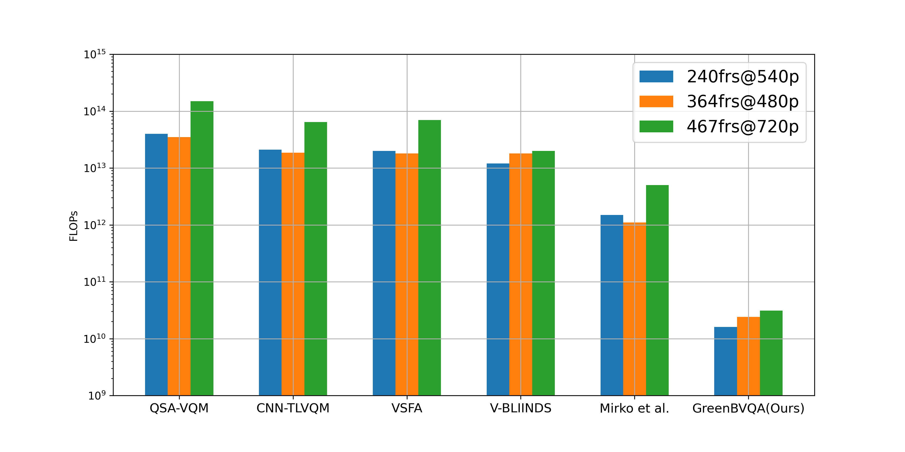
Figure 6: Comparison of the floating point operation (FLOP) numbers.

4.3.3 Computational complexity

The number of floating point operations (FLOPs) provides another way to assess the complexity of a BVQA model. We estimate the FLOPs of several DL-based BVQA methods required to predict video quality score and compare them with that of GreenBVQA. The FLOPs required by one 240frs@540p test video in the KoNViD-1k dataset are shown in the last column of Table 9. QSA-VQM, CNN-TLVQM, and VSFA demand remarkably higher FLOPs numbers, ranging from 1250 to 2500 times of GreenBVQA. Mirko et al., which is an efficient BVQA method specifically designed to reduce inference time and computational complexity, still requires about 100 times of GreenBVQA.

To be consistent with the inference time analysis, three test videos of different lengths and resolutions are selected for FLOPs comparison in Fig. 6. FLOPS are shown as a function of the frame number and resolution for several benchmarking methods. For all the three videos, QSA-VQM, CNN-TLVQM, VSFA, and V-BLIINDS demand a much larger number of FLOPs than GreenBVQA. As an efficient method of BVQA, Mirko et al. reduce FLOPs a lot, while still requiring FLOPs of two orders of magnitude against GreenBVQA. On the other hand, this discrepancy is not reflected by the inference time comparison in Table 10 since DL-based methods benifit a lot from mature coding libraries and environments adept at facilitating deep learning computations. The extremetly low FLOPs suggests the potential for future enhancements in computational efficiency, further bolstering the appeal of GreenBVQA for real-time video quality assessment tasks in the edge computing realm.

Table 11: Ablation Study for GreenBVQA.

	CVD2014		LIVE-VQC		KoNViD-1k
Model	SRCC	PLCC	SRCC	PLCC	SRCC	PLCC
S features	0.809	0.844	0.728	0.758	0.720	0.724
S+T features	0.835	0.854	0.762	0.771	0.742	0.749
S+T+ST features	-	-	0.776	0.781	0.765	0.766
S+T+ST+SC features	-	-	0.785	0.789	0.776	0.779

4.4 Abalation Study

We conduct an ablation study on the choice of selected features in GreenBVQA. The results are reported in Table 11. The examined features include spatial features (S-features), temporal features (T-features), spatio-temporal features (ST-features), and spatio-color features (SC-features). Our study begins with the assessment of the effectiveness of spatial features (the first row), followed by adding temporal features (the second row). We see that both SROCC and PLCC improve in all three datasets. The addition of ST-features (the third row) can improve SROCC and PLCC for all datasets as well. Finally, we use all four feature types and observe further improvement in SROCC and PLCC (the last row). Note that the performance of ST and SC features is not reported for the CVD2014 dataset since their improvement is little. A combination of S and T features already reaches high performance for this dataset.

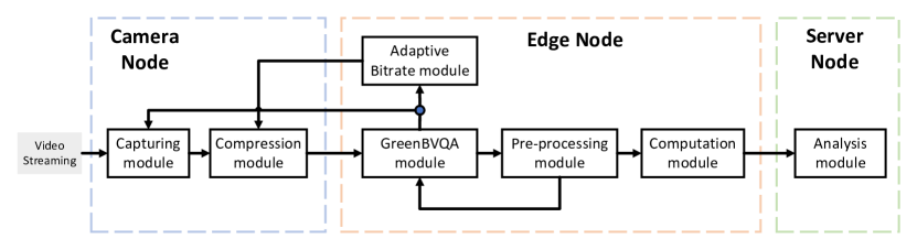
Figure 7: Illustration of an edge computing system employing GreenBVQA.

5 An Edge Computing System with BVQA

In this section, we introduce a video-based edge computing system to illustrate the role of GreenBVQA in facilitating various video processing tasks at the edge. Existing bitrate adaptive video augmentation methods [55] primarily consider the tradeoff between video bitrate and bandwidth consumption to improve the quality of experience. Yet, most of them ignore the perceptual quality of streaming videos. Perceptual video quality is more relevant to the human visual experience. A video with higher bitrates does not guarantee perceptual friendliness due to the presence of perceptual distortions such as blurriness, noise, blockiness, etc. Although the FR-VQA technique can account for the perceptual quality of streaming video, the resulting methods rely on reference videos, which are not available on edge or mobile devices. As a blind video quality assessment method, GreenBVQA can operate without any reference. Its small model size and low computational complexity make it well-suited for deployment on edge devices. Furthermore, its energy efficiency and cost-effectiveness, evidenced by short inference time, support its applicability in an edge computing system.

GreenBVQA can be used as a perceptual quality monitor on edge devices. An edge computing system that employs GreenBVQA is shown in Fig. 7, where GreenBVQA is used to enhance users’ experience in watching videos. As shown in the figure, the system involves predicting the perceptual quality of video streams with no reference. The predicted quality score can be utilized by other modules in the system.

1. The predicted score can be used as feedback to the phone camera in video capturing. In certain extreme situations, such as dark or blurred video capturing conditions, a low predicted video quality score can serve as an alert so that the user can change the camera setting to get improved video quality.

2. In the context of video streaming over the network, it can assist the adaptive bitrate module in adjusting the bitrate of subsequent video streams. If the predicted score is higher, the coding module at the transmitter end can provide a lower bitrate video stream to save the bandwidth.

3. Several video pre-processing modules (e.g., video enhancement [56] and video denoising [57]) are commonly implemented on edge devices to alleviate the computational burden of the server. By leveraging the predicted video quality scores, unnecessary pre-processing operations can be saved. For instance, when a sequence of video frames is predicted to have a good visual quality, there is no need to denoise or deblur the frame sequence. GreenBVQA can also be used to evaluate the performance of video pre-processing tasks.

6 Conclusion and Future Work

As the demand for high-quality videos captured and consumed at the edge continues to grow, there is an urgent need for a perceptual video quality prediction model that can guide these tasks effectively. A lightweight blind video quality assessment method called GreenBVQA was proposed in this work. Its SROCC and PLCC prediction performance was evaluated on three popular video quality assessment datasets. GreenBVQA outperforms all conventional (non-DL-based) BVQA methods and achieves comparable performance with state-of-the-art (DL-based) BVQA methods. GreenBVQA’s small model size and low computational complexity, which implies high energy efficiency, make it well-suited for integration into an edge-based video system. GreenBVQA exhibits short inference times, enabling real-time prediction of perceptual video quality scores using either CPUs or GPUs.

There are several promising research directions worth future investigation. First, in the context of high frame rate video capturing and transmission, it is desired to adopt adaptive bitrate (ABR) video with variable frame rates (VFR). With the emergence of advanced edge devices capable of capturing high frame rate videos, we expect GreenBVQA to support VFR video and enable ABR video transmission with proper adaptation. Second, as user-generated content (UGC) videos with diverse content grow, we see a need to tailor GreenBVQA to specific content types such as gaming and virtual reality (VR).

References

- [1] Zhi Li, Anne Aaron, Ioannis Katsavounidis, Anush Moorthy, and Megha Manohara. Toward a practical perceptual video quality metric. The Netflix Tech Blog, 6(2):2, 2016.
- [2] Joe Yuchieh Lin, Tsung-Jung Liu, Eddy Chi-Hao Wu, and C-C Jay Kuo. A fusion-based video quality assessment (fvqa) index. In Signal and Information Processing Association Annual Summit and Conference (APSIPA), 2014 Asia-Pacific, pages 1–5. IEEE, 2014.
- [3] Rajiv Soundararajan and Alan C Bovik. Video quality assessment by reduced reference spatio-temporal entropic differencing. IEEE Transactions on Circuits and Systems for Video Technology, 23(4):684–694, 2012.
- [4] Anish Mittal, Rajiv Soundararajan, and Alan C Bovik. Making a completely blind image quality analyzer. IEEE Signal processing letters, 20(3):209–212, 2012.
- [5] Anush Krishna Moorthy and Alan Conrad Bovik. Blind image quality assessment: From natural scene statistics to perceptual quality. IEEE transactions on Image Processing, 20(12):3350–3364, 2011.
- [6] Anish Mittal, Anush Krishna Moorthy, and Alan Conrad Bovik. No-reference image quality assessment in the spatial domain. IEEE Transactions on image processing, 21(12):4695–4708, 2012.
- [7] Peng Ye, Jayant Kumar, Le Kang, and David Doermann. Unsupervised feature learning framework for no-reference image quality assessment. In 2012 IEEE conference on computer vision and pattern recognition, pages 1098–1105. IEEE, 2012.
- [8] Jingtao Xu, Peng Ye, Qiaohong Li, Haiqing Du, Yong Liu, and David Doermann. Blind image quality assessment based on high order statistics aggregation. IEEE Transactions on Image Processing, 25(9):4444–4457, 2016.
- [9] Sebastian Bosse, Dominique Maniry, Klaus-Robert Müller, Thomas Wiegand, and Wojciech Samek. Deep neural networks for no-reference and full-reference image quality assessment. IEEE Transactions on image processing, 27(1):206–219, 2017.
- [10] Yu Zhang, Xinbo Gao, Lihuo He, Wen Lu, and Ran He. Blind video quality assessment with weakly supervised learning and resampling strategy. IEEE Transactions on Circuits and Systems for Video Technology, 29(8):2244–2255, 2018.
- [11] Giuseppe Valenzise, Stefano Magni, Marco Tagliasacchi, and Stefano Tubaro. No-reference pixel video quality monitoring of channel-induced distortion. IEEE transactions on circuits and systems for video technology, 22(4):605–618, 2011.
- [12] Jacob Søgaard, Søren Forchhammer, and Jari Korhonen. No-reference video quality assessment using codec analysis. IEEE Transactions on Circuits and Systems for Video Technology, 25(10):1637–1650, 2015.
- [13] Michele A Saad, Alan C Bovik, and Christophe Charrier. Blind prediction of natural video quality. IEEE Transactions on Image Processing, 23(3):1352–1365, 2014.
- [14] Anish Mittal, Michele A Saad, and Alan C Bovik. A completely blind video integrity oracle. IEEE Transactions on Image Processing, 25(1):289–300, 2015.
- [15] Yongxu Liu, Jinjian Wu, Leida Li, Weisheng Dong, Jinpeng Zhang, and Guangming Shi. Spatiotemporal representation learning for blind video quality assessment. IEEE Transactions on Circuits and Systems for Video Technology, 32(6):3500–3513, 2021.
- [16] Jia Deng, Wei Dong, Richard Socher, Li-Jia Li, Kai Li, and Li Fei-Fei. Imagenet: A large-scale hierarchical image database. In 2009 IEEE conference on computer vision and pattern recognition, pages 248–255. Ieee, 2009.
- [17] Dingquan Li, Tingting Jiang, and Ming Jiang. Unified quality assessment of in-the-wild videos with mixed datasets training. International Journal of Computer Vision, 129(4):1238–1257, 2021.
- [18] Zhengzhong Tu, Xiangxu Yu, Yilin Wang, Neil Birkbeck, Balu Adsumilli, and Alan C Bovik. Rapique: Rapid and accurate video quality prediction of user generated content. IEEE Open Journal of Signal Processing, 2:425–440, 2021.
- [19] Abdelhak Bentaleb, Bayan Taani, Ali C Begen, Christian Timmerer, and Roger Zimmermann. A survey on bitrate adaptation schemes for streaming media over http. IEEE Communications Surveys & Tutorials, 21(1):562–585, 2018.
- [20] Pooyan Safari, Behnam Shariati, David Przewozny, Paul Chojecki, Johannes Karl Fischer, Ronald Freund, Axel Vick, and Moritz Chemnitz. Edge cloud based visual inspection for automatic quality assurance in production. In 2022 13th International Symposium on Communication Systems, Networks and Digital Signal Processing (CSNDSP), pages 473–476. IEEE, 2022.
- [21] Yutong Liu, Linghe Kong, Guihai Chen, Fangqin Xu, and Zhanquan Wang. Light-weight ai and iot collaboration for surveillance video pre-processing. Journal of Systems Architecture, 114:101934, 2021.
- [22] C-C Jay Kuo and Azad M Madni. Green learning: Introduction, examples and outlook. Journal of Visual Communication and Image Representation, page 103685, 2022.
- [23] C-C Jay Kuo. Understanding convolutional neural networks with a mathematical model. Journal of Visual Communication and Image Representation, 41:406–413, 2016.
- [24] Zhanxuan Mei, Yun-Cheng Wang, Xingze He, and C-C Jay Kuo. Greenbiqa: A lightweight blind image quality assessment method. In 2022 IEEE 24th International Workshop on Multimedia Signal Processing (MMSP), pages 1–6. IEEE, 2022.
- [25] Yijing Yang, Wei Wang, Hongyu Fu, and C-C Jay Kuo. On supervised feature selection from high dimensional feature spaces. arXiv preprint arXiv:2203.11924, 2022.
- [26] Mariette Awad and Rahul Khanna. Support vector regression. In Efficient learning machines, pages 67–80. Springer, 2015.
- [27] Tianqi Chen and Carlos Guestrin. Xgboost: A scalable tree boosting system. In Proceedings of the 22nd acm sigkdd international conference on knowledge discovery and data mining, pages 785–794, 2016.
- [28] Michele A Saad and Alan C Bovik. Blind quality assessment of videos using a model of natural scene statistics and motion coherency. In 2012 Conference Record of the Forty Sixth Asilomar Conference on Signals, Systems and Computers (ASILOMAR), pages 332–336. IEEE, 2012.
- [29] Xuelong Li, Qun Guo, and Xiaoqiang Lu. Spatiotemporal statistics for video quality assessment. IEEE Transactions on Image Processing, 25(7):3329–3342, 2016.
- [30] Sathya Veera Reddy Dendi and Sumohana S Channappayya. No-reference video quality assessment using natural spatiotemporal scene statistics. IEEE Transactions on Image Processing, 29:5612–5624, 2020.
- [31] Jingtao Xu, Peng Ye, Yong Liu, and David Doermann. No-reference video quality assessment via feature learning. In 2014 IEEE international conference on image processing (ICIP), pages 491–495. IEEE, 2014.
- [32] Jari Korhonen. Two-level approach for no-reference consumer video quality assessment. IEEE Transactions on Image Processing, 28(12):5923–5938, 2019.
- [33] Kede Ma, Wentao Liu, Kai Zhang, Zhengfang Duanmu, Zhou Wang, and Wangmeng Zuo. End-to-end blind image quality assessment using deep neural networks. IEEE Transactions on Image Processing, 27(3):1202–1213, 2017.
- [34] Wentao Liu, Zhengfang Duanmu, and Zhou Wang. End-to-end blind quality assessment of compressed videos using deep neural networks. In ACM Multimedia, pages 546–554, 2018.
- [35] Chunfeng Wang, Li Su, and Weigang Zhang. Come for no-reference video quality assessment. In 2018 IEEE Conference on Multimedia Information Processing and Retrieval (MIPR), pages 232–237. IEEE, 2018.
- [36] Junyong You and Jari Korhonen. Deep neural networks for no-reference video quality assessment. In 2019 IEEE International Conference on Image Processing (ICIP), pages 2349–2353. IEEE, 2019.
- [37] Dingquan Li, Tingting Jiang, and Ming Jiang. Quality assessment of in-the-wild videos. In Proceedings of the 27th ACM International Conference on Multimedia, pages 2351–2359, 2019.
- [38] Zhenqiang Ying, Maniratnam Mandal, Deepti Ghadiyaram, and Alan Bovik. Patch-vq:’patching up’the video quality problem. In Proceedings of the IEEE/CVF Conference on Computer Vision and Pattern Recognition, pages 14019–14029, 2021.
- [39] Mirko Agarla, Luigi Celona, and Raimondo Schettini. No-reference quality assessment of in-capture distorted videos. Journal of Imaging, 6(8):74, 2020.
- [40] Jari Korhonen, Yicheng Su, and Junyong You. Blind natural video quality prediction via statistical temporal features and deep spatial features. In Proceedings of the 28th ACM International Conference on Multimedia, pages 3311–3319, 2020.
- [41] Xuan Qi and Chen Liu. Enabling deep learning on iot edge: Approaches and evaluation. In 2018 IEEE/ACM Symposium on Edge Computing (SEC), pages 367–372. IEEE, 2018.
- [42] Zhujun Xiao, Zhengxu Xia, Haitao Zheng, Ben Y Zhao, and Junchen Jiang. Towards performance clarity of edge video analytics. In 2021 IEEE/ACM Symposium on Edge Computing (SEC), pages 148–164. IEEE, 2021.
- [43] Jiasi Chen and Xukan Ran. Deep learning with edge computing: A review. Proceedings of the IEEE, 107(8):1655–1674, 2019.
- [44] Chien-Chun Hung, Ganesh Ananthanarayanan, Peter Bodik, Leana Golubchik, Minlan Yu, Paramvir Bahl, and Matthai Philipose. Videoedge: Processing camera streams using hierarchical clusters. In 2018 IEEE/ACM Symposium on Edge Computing (SEC), pages 115–131. IEEE, 2018.
- [45] Jongwon Yoon and Suman Banerjee. Hardware-assisted, low-cost video transcoding solution in wireless networks. IEEE Transactions on Mobile Computing, 19(3):581–597, 2019.
- [46] Zhengfang Duanmu, Wentao Liu, Zhuoran Li, Diqi Chen, Zhou Wang, Yizhou Wang, and Wen Gao. Assessing the quality-of-experience of adaptive bitrate video streaming. arXiv preprint arXiv:2008.08804, 2020.
- [47] Mirko Agarla, Luigi Celona, and Raimondo Schettini. An efficient method for no-reference video quality assessment. Journal of Imaging, 7(3):55, 2021.
- [48] Andrew G Howard, Menglong Zhu, Bo Chen, Dmitry Kalenichenko, Weijun Wang, Tobias Weyand, Marco Andreetto, and Hartwig Adam. Mobilenets: Efficient convolutional neural networks for mobile vision applications. arXiv preprint arXiv:1704.04861, 2017.
- [49] Zhanxuan Mei, Yun-Cheng Wang, Xingze He, Yong Yan, and C-C Jay Kuo. Lightweight high-performance blind image quality assessment. arXiv preprint arXiv:2303.13057, 2023.
- [50] C-C Jay Kuo, Min Zhang, Siyang Li, Jiali Duan, and Yueru Chen. Interpretable convolutional neural networks via feedforward design. Journal of Visual Communication and Image Representation, 60:346–359, 2019.
- [51] Vlad Hosu, Franz Hahn, Mohsen Jenadeleh, Hanhe Lin, Hui Men, Tamás Szirányi, Shujun Li, and Dietmar Saupe. The konstanz natural video database (konvid-1k). In 2017 Ninth international conference on quality of multimedia experience (QoMEX), pages 1–6. IEEE, 2017.
- [52] Mikko Nuutinen, Toni Virtanen, Mikko Vaahteranoksa, Tero Vuori, Pirkko Oittinen, and Jukka Häkkinen. Cvd2014—a database for evaluating no-reference video quality assessment algorithms. IEEE Transactions on Image Processing, 25(7):3073–3086, 2016.
- [53] Zeina Sinno and Alan Conrad Bovik. Large-scale study of perceptual video quality. IEEE Transactions on Image Processing, 28(2):612–627, 2018.
- [54] Zhengzhong Tu, Yilin Wang, Neil Birkbeck, Balu Adsumilli, and Alan C Bovik. Ugc-vqa: Benchmarking blind video quality assessment for user generated content. IEEE Transactions on Image Processing, 30:4449–4464, 2021.
- [55] Yusuf Sani, Andreas Mauthe, and Christopher Edwards. Adaptive bitrate selection: A survey. IEEE Communications Surveys & Tutorials, 19(4):2985–3014, 2017.
- [56] Yirui Wu, Haifeng Guo, Chinmay Chakraborty, Mohammad Khosravi, Stefano Berretti, and Shaohua Wan. Edge computing driven low-light image dynamic enhancement for object detection. IEEE Transactions on Network Science and Engineering, 2022.
- [57] Liming Ge, Wei Bao, Dong Yuan, and Bing B Zhou. Edge-assisted deep video denoising and super-resolution for real-time surveillance at night. In Proceedings of the 28th Annual International Conference on Mobile Computing And Networking, pages 783–785, 2022.