Gradient-type subspace iteration methods for the symmetric eigenvalue problem

Abstract

This paper explores variants of the subspace iteration algorithm for computing approximate invariant subspaces. The standard subspace iteration approach is revisited and new variants that exploit gradient-type techniques combined with a Grassmann manifold viewpoint are developed. A gradient method as well as a conjugate gradient technique are described. Convergence of the gradient-based algorithm is analyzed and a few numerical experiments are reported, indicating that the proposed algorithms are sometimes superior to a standard Chebyshev-based subspace iteration when compared in terms of number of matrix vector products, but do not require estimating optimal parameters. An important contribution of this paper to achieve this good performance is the accurate and efficient implementation of an exact line search. In addition, new convergence proofs are presented for the non-accelerated gradient method that includes a locally exponential convergence if started in a $\mathcal{O}(\sqrt{\delta})$ neighbourhood of the dominant subspace with spectral gap $\delta$.

Keywords: Invariant subspaces; Eigenspaces; Partial diagonalization; Grassmann Manifolds; Gradient descent; Trace optimization. AMS: 15A69, 15A18

1 Introduction

When considering the many sources of large eigenvalue problems in numerical linear algebra, one often observes that the actual underlying problem it to compute an invariant subspace. In these cases, the eigenvalues and eigenvectors are often a by-product of the computations and they are not directly utilized. For example, one of the most common calculations in data science consists of performing a dimension reduction which extracts a subspace that provides a good approximation of the original data in that not much information is lost when we project the original problem into this low-dimensional space. This projection often results in better accuracy since the information that is shed out corresponds to noise. Another example is in electronic structure calculations where an important class of algorithms called ‘linear scaling methods’ are entirely based on the eigenprojector on the subspace associated with the ‘occupied states’. This projector is available through any orthonormal basis of the invariant subspace and here again eigenvectors and eigenvalues are not explicitly needed, resulting in methods that scale linearly with the number of particles.

While this distinction is often blurred in the literature, a number of articles did specifically deal with the problem of computing an invariant subspace by expressing it in terms of computing objects on the Grassmann manifold. Thus, the well-known article [12] addressed general optimization problems on manifolds, including eigenvalue problems as a special case. A number of other papers also adopted, explicitly or implicitly, a matrix manifold viewpoint for computing invariant subspaces, see, e.g., [1, 8, 20, 7, 4, 3, 5], among others. In many of these contributions, a Newton-type approach is advocated to solve the resulting equations. Newton’s method typically requires solving linear systems, or a sequence of Sylvester equations and this can be quite expensive, or even impractical in some situations.

In view of the above observation, we may ask whether or not a gradient approach can yield an effective alternative to standard implementations of subspace iteration. Subspace Iteration (SI) computes the dominant invariant subspace of a matrix and some of its known advantages are highly desirable in a number of situations. SI is a block form of the power method and as such it is rather simple to implement. It is also known for its robustness properties. For example, it is resilient to small changes in the matrix during iteration, an important attribute that is not shared by Krylov subspace methods. This particular feature is appealing in many practical instances as in, e.g, subspace tracking [15, 13, 11, 22, 9], or in electronic structure calculations [24, 25].

This paper considers variations of subspace iteration that are grounded in a gradient-type method on the Grassmann manifold. A gradient and a (nonlinear) conjugate gradient approach are described that both share the same advantages as those of classical SI. However, the proposed methods are based on a direct optimization of the partial trace of the matrix in the subspace. The convergence of the gradient algorithm will be studied theoretically.

We point out that other gradient-descent type methods that employ a Grassmannian viewpoint have been recently developed in [4, 5]. These methods differ from those of this paper in that they aim at following a geodesic on the manifold by exploiting a Riemannian structure. No such attempt is made in the methods proposed herein. Instead, a simple gradient descent (or ascent) approach with (exact) line search is applied and a retraction step is added to ensure the orthogonality of the basis of the new subspace.

The first part of the paper discusses classical versions of subspace iteration. The second part develops line-search techniques combined with gradient descent-type approaches. A conjugate gradient approach is also presented.

2 Background and notation

This section begins with providing some background on invariant subspaces and then defines the notation to be used throuhgout the paper.

2.1 Invariant subspaces

Given an $n\times n$ matrix $A$, a subspace ${\cal X}$ that is invariant with respect to $A$ is a subspace of dimension $p$ of $\mathbb{R}^{n}$ such that:

$$A{\cal X}\subseteq{\cal X}.$$ (1)

This can be expressed in matrix form by using a basis $X\in\mathbb{R}^{n\times p}$ of ${\cal X}$. In this case ${\cal X}$ is invariant iff there exists a matrix $\Lambda\in\mathbb{R}^{p\times p}$ such that

$$AX=X\Lambda.$$ (2)

This second definition depends on a basis which is not unique. Herein lies a conundrum that is encountered in this context. We need a (non-unique) basis for computations and expressing equations and equalities; however, the original definition (1) does not require a basis.

We will sometimes use the term ‘eigenspace’ to mean invariant subspaces. The terminology used varies as eigenspaces are often restricted to mean the invariant subspace associated with one eigenvalue instead of a group of eigenvalues.

A number of computational tasks deal specifically with invariant subspaces. The most common of these is probably just to compute an invariant subspace as represented by, e.g., an orthonormal basis. Sometimes, the task is to update the subspace rather than compute it from scratch. This happens for example when solving the Kohn–Sham equation, see e.g., [19] in electronic structure calculations where at each iteration of the Self-Consistent Field (SCF) method the Hamiltonian changes slightly and it is necessary to update an already computed approximate invariant subspace for the previous Hamiltonian. There are also numerous applications in signal processing, where the problem is to track an invariant subspace of a sequence of matrices, see e.g., [22, 11, 16, 13] a problem that is somewhat related to subspace updating problem.

Another problem that is often encountered is to (inexpensively) estimate the dimension of some invariant subspace. Thus, the approximate rank or numerical rank of some data matrix can be needed in order to determine the proper dimension required for an adequate “dimension reduction”, or for subspace tracking [16]. This numerical rank can be determined as the dimension of the (near) invariant subspace corresponding to singular values larger than a certain threshold $\epsilon$, see, e.g., [23]. Another problem in signal processing, is to find a subspace that is simultaneously a near-invariant subspace for a set of matrices. A common characteristic of the examples just mentioned is that they all deal with invariant subspaces – but they do not require eigenvalues and vectors explicitly.

2.2 Notation and assumptions

For the remainder of the paper we will restrict our attention to the case when $A$ is real symmetric and positive definite. The positive-definiteness assumption is made for theoretical reasons and without loss of generality since the iterates produced by the algorithms in this paper are invariant to the transformation $A+cI$ for real $c$. In addition, we will consider the problem of computing the invariant subspace associated with the largest $p$ eigenvalues, which we refer to as the $p$th “dominant” subspace. In case the subspace that corresponds to the smallest $p$ eigenvalues is sought, the algorithms can be applied to $-A$.

Given an $n\times n$ symmetric real matrix $A$, we denote by $\lambda_{1}\geq\lambda_{2}\geq\cdots\geq\lambda_{n}$ its eigenvalues counted with their multiplicities.

A common method for finding the $p$th dominant subspace of $A$ consists of minimizing the function

$$\phi(X)=-\frac{1}{2}\operatorname{Tr}(X^{T}AX),$$ (3)

over the set of $n\times p$ matrices with orthonormal columns, i.e., such that $X^{T}X=I$, see for example, [20, 21, 2, 12]. In general, non-zero spectral gap will be assumed,

$$\delta=\lambda_{p}-\lambda_{p+1}>0.$$ (4)

This condition implies that there exists a unique dominant subspace associated with the $p$ largest eigenvalues of $A$. Thus, minimizing the objective $\phi$ has a unique solution.

We denote by $\texttt{Diag}(A)$ the diagonal matrix whose diagonal entries are the same as those of $A$. The notation is overloaded by defining $\texttt{Diag}(\alpha_{i})_{i=1:n}$ to be the diagonal matrix with diagonal entries $\alpha_{i},i=1:n$. This dual use of $\texttt{Diag}(.)$ causes no ambiguity and is consistent with common usage as, for example, in Matlab.

2.3 Subspace iteration

Given some initial subspace with a basis $X_{0}\in\mathbb{R}^{n\times p}$, the classical subspace iteration algorithm is nothing but a Rayleigh-Ritz projection method onto the subspace spanned by $X_{k}=A^{k}X_{0}$. That is, we seek an approximate eigenpair $\tilde{\lambda},\tilde{u}$ where $\tilde{\lambda}\ \in\ \mathbb{R}$ and $\tilde{u}\ \in\ \text{Span}{(X_{k})}$, by requiring that $(A-\tilde{\lambda}I)\tilde{u}\perp\text{Span}{(X_{k})}$. If $Q=[q_{1},\ldots,q_{m}]$ is an orthonormal basis of $X_{k}$, and we express the approximate eigenvector as $\tilde{u}=Q\tilde{y}$, then this leads to $Q^{T}(A-\tilde{\lambda}I)\tilde{u}=0$ which means that $\tilde{\lambda},\tilde{y}$ is the solution of the projected eigenvalue problem

$$Q^{T}AQ\tilde{y}=\tilde{\lambda}\tilde{y}.$$ (5)

A common and more effective alternative is to define $X_{k}$ to be of the form $X_{k}=p_{k}(A)X_{0}$, in which $p_{k}$ is some optimally selected polynomial of degree $k$. The original form discussed above which was described by Bauer [6], corresponds to using the monomial $p_{k}(t)\equiv t^{k}$ or the shifted monomial $p_{k}(t)=(t-c)^{k}$. Rutishauser later developed more advanced versions in which $p_{k}(t)$ was selected to be a shifted and scaled Chebyshev polynomial [17, 18].

Algorithm 1 $[X_{new},D]$ = SubsIt$(A,X)$

1:Start: Select initial system $X=\left[x_{1},\ldots,x_{p}\right]$ and initial polynomial $p_{k}$.

2:for iter=1:MaxIts do

3:     Compute $\hat{X}=p_{k}(A)X$;  $Q=qr(\hat{X})$;  and   $C=Q^{T}AQ$.

4:     Diagonalize $C$ as $C=U\Lambda_{C}U^{T}$ and set $X_{new}=QU$

5:     if convergence satisfied then

6:         return

7:     else

8:         Set $X:=X_{new}$ and select a new polynomial $p^{\prime}_{k^{\prime}}$

9:     end if

10:end for

The optimal polynomial

An important issue when applying subspace iteration, is to select an optimal polynomial $p_{k}(t)$ to use. Consider a spectrum of $A$ as in Figure 1. Assuming that we use a subspace of dimension $m$, the polynomial is selected so as to enable the method to compute the eigenvalues $\lambda_{1},\lambda_{2},\ldots,\lambda_{p}$. The standard approach [17] for subspace iteration when computing the dominant subspace is to use the polynomial

$$p_{k}(t)\equiv C_{k}((t-c)/h)\quad\text{where $c=(\lambda_{p+1}+\lambda_{n})/2$ and $h=(\lambda_{p+1}-\lambda_{n})/2$}.$$ (6)

Here, $C_{k}(t)$ is the Chebyshev polynomial of the first kind of degree $k$. Remark that $c$ is the middle of the interval $[\lambda_{n},\ \lambda_{p+1}]$ of unwanted eigenvalues, and $h$ is half the width of this interval.

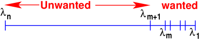
Figure 1: Typical scenario for subspace iteration

Figure 2: Polynomial used in the context of subspace iteration.

The polynomial above is found from an analysis of subspace iteration that reveals that, when considering each eigenpair $\lambda_{i},u_{i}$ for $i\leq m$, the method acts as if the other eigenvalues $\lambda_{j},j<p,j\neq i$ are not present. In other words, the polynomial is selected with the aim to minimize the maximum $p_{k}(\lambda_{k})/p_{k}(\lambda_{i})$ for $k>p$ over polynomials of degree $k$. This is then relaxed to minimizing the maximum of $p_{k}(t)/p_{k}(\lambda_{i})$ for $t\in\ [\lambda_{p+1},\lambda_{n}]$ over polynomials of degree $k$. The optimal polynomial is $C_{k}((t-c)/h)/C_{k}((\lambda_{i}-c)/h)$ where the denominator is for scaling purposes. In practice $\lambda_{p+1},\ldots,\lambda_{n}$ are estimated and the scaling is performed for $i=1$, i.e., with $\lambda_{1}$ which is also estimated [17, 18]. Note that this polynomial is optimal for each eigenvalue $\lambda_{j},j\leq p$, individually. However, it is not optimal when considering the subspace as a whole: a few experiments will reveal that convergence can be much faster when we replace $\lambda_{p+1}$ in the definition of polynomial by $\lambda_{p+k}$ for some $k>1$. Note that there does not seem to be a theoretical study of this empirical observation. Our numerical experiments will illustrate this room for improvement further.

Comparison with Krylov subspace methods

It is known that when computing a small number of eigenvalues and vectors at one end of the spectrum, Krylov subspace methods such as the Lanczos method and Arnoldi’s method are generally faster than methods based on subspace iteration. Standard Krylov methods require only one starting vector and this can be seen as an advantage in that little data needs to be generated to start the algorithm. However, for many applications it can be a disadvantage. Indeed, there are applications where a subspace must be computed repeatedly of a matrix that changes slightly from step to step. At the start of a new iteration we have available the whole (orthonormal) basis from the previous iteration which should be exploited. However, since Krylov methods start with only one vector this is not possible. In addition, Krylov methods do not have a fixed computational cost per iteration since they grow the subspace in each step.

On the other hand, the subspace iteration algorithm is perfectly suitable for the situation just described: When a computation with a new matrix starts, we can take in the algorithm as initial subspace the latest subspace obtained from the previous matrix. This is the exact scenario encountered in electronic structure calculations [24, 25], where a subspace is to be computed at each SCF iteration. The matrix changes at each SCF iteration and the changes depend on the eigenvectors and eigenvalues obtained at the previous SCF step.

3 Invariant subspaces and the Grassmannian perspective

An alternative to using subspace iteration for computing a dominant invariant subspace is to consider a method whose goal is to optimize the objective function $\phi(X)$, defined in (3), over all matrices $X$ that have orthonormal columns. This idea is of course not new. For example, it is the main ingredient exploited in the TraceMin algorithm [20, 21], a method designed for computing an invariant subspace associated with smallest eigenvalues for standard and generalized eigenvalue problems.

A key observation in the definition (3) is that $\phi(X)$ is invariant upon orthogonal transformations. In other words if $W$ is a $p\times p$ orthogonal matrix then, $\phi(XW)=\phi(X)$. Noting that two orthonormal bases $X_{1}$ and $X_{2}$ of the same subspace are related by $X_{2}=X_{1}W$ where $W$ is some orthogonal $p\times p$ matrix, this means that the objective function (3) depends only on the subspace spanned by $X$ and not the particular orthonormal basis $X$ employed to represent the subspace. This in turn suggests that it is possible, and possibly advantageous, to seek the optimum solution in the Grassmann manifold [12]. Recall, from e.g., [12], that the Stiefel manifold is the set

$$\textnormal{St}(n,p)=\{X\ \in\ \mathbb{R}^{n\times p}\colon\ X^{T}X=I\}.$$ (7)

while the Grassmann manifold is the quotient manifold

$$\operatorname{Gr}(n,p)=\textnormal{St}(n,p)/\textnormal{O}(p)$$ (8)

where $\textnormal{O}(p)$ is the orthogonal group of unitary $p\times p$ matrices. Each point on the manifold, one of the equivalence classes in the above definition, can be viewed as a subspace of dimension $p$ of $\mathbb{R}^{n}$. In other words,

$$\operatorname{Gr}(n,p)=\{\mathcal{X}\subseteq\mathbb{R}^{n}\colon\mathcal{X}\hskip 2.84526pt\text{is a subspace of}\dim(\mathcal{X})=p\}.$$ (9)

An element of $\operatorname{Gr}(n,p)$ can be indirectly represented by a basis $X\in\textnormal{St}(n,p)$ modulo an orthogonal transformation and so we denote it by $[X]$, keeping in mind that it does not matter which member $X$ of the equivalence class is selected for this representation.

With this Riemannian viewpoint in mind, one can try to minimize $\phi(X)$ over the Grassmann manifold using one of the many (generic) Riemannian optimization algorithms for smooth optimization. One has, for example, first-order and second-order algorithms that generalize gradient descent and Newton’s iteration, resp. We refer to the foundational article [12] and the textbook [2] for detailed explanations. Despite its algorithmic simplicity, the Riemanian gradient method for this problem has not been treated in much detail beyond the basic formulation and its generically applicable theoretical properties. In the next sections, our aim it to work this out in detail and show in the numerical experiments that such a first-order method can be surprisingly effective and competitive.

3.1 Gradient method on Grassmann

In a gradient approach we would like to produce an iterate $X_{k+1}\in\mathbb{R}^{n\times p}$ starting from $X_{k}\in\mathbb{R}^{n\times p}$ following a rule of the form

$$X_{k+1}=X_{k}-\mu\operatorname{grad}\phi(X_{k}),$$ (10)

where the step $\mu>0$ is to be determined by some linesearch. The direction opposite to the gradient is a direction of decrease for the objective function $\phi$. However, it is unclear what value of the step $\mu$ yields the largest decrease in the value of $\phi$. This means that some care has to be exercised in the search for the optimal $\mu$. A gradient procedure may be appealing if a good approximate solution is already known, in which case, the gradient algorithm may provide a less expensive alternative to one step of the subspace iteration 1.

For a Riemannian method defined on a manifold, the search direction (here, $-\operatorname{grad}\phi(X_{k})$) always lies in the tangent space of the current point (here, $X_{k}$) of said manifold. This makes sense since directions orthogonal to the tangent space leave the objective function constant up to first order in the step if the iterates are restricted to lie on the manifold. For our problem, an element of the Grassmann manifold is represented by a member $X\in\textnormal{St}(n,p)$ of its class. The tangent space of the Grassmann manifold at this $[X]$ is the set of matrices $\Delta\in\mathbb{R}^{n\times p}$ satisfying the following orthogonality relation, see [12]:

$$X^{T}\Delta=0.$$ (11)

The Riemannian gradient of (3) at $[X]$ is

$$\operatorname{grad}\phi(X)=-\Pi AX\equiv-(AX-XC_{X}),$$ (12)

with the orthogonal projector $\Pi=I-XX^{T}$, and the projected matrix $C_{X}=X^{T}AX$.

Even though $\operatorname{grad}\phi(X_{k})$ is in the tangent space (and a direction of decrease for $\phi$), we are not interested in $X_{k+1}$ per se but in the subspace that it spans. In particular, since we use orthogonal bases to define the value of $\phi$ on the manifold, we will need to ‘correct’ the non-orthogonality of the update (10) when considering $\phi$. This will be discussed shortly. For now we establish a few simple relations.

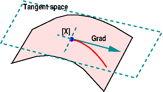
Figure 3: Illustration of the line-search and the tangent space

For simplicity we denote $X:=X_{k}$ an orthonormal basis of the current iterate, $\tilde{X}:=X_{k+1}$ a (probably non-orthonormal) basis of the new iterate and $G:=\operatorname{grad}\phi(X)$ the gradient direction. Then a step of the gradient method satisfies $\tilde{X}=X-\mu G$ and a short calculation will show that

$$\phi(\tilde{X})=\phi(X)-\mu\operatorname{Tr}((AX)^{T}\Pi(AX))-\frac{\mu^{2}}{2}\operatorname{Tr}((AX)^{T}\Pi A\Pi(AX)).$$ (13)

We also have the following relations

$$(AX)^{T}\Pi(AX) = -(AX)^{T}G=-(G^{T}(AX))^{T}=-G^{T}(AX)$$ (14)

$$= (AX)^{T}\Pi^{T}\Pi(AX)=G^{T}G$$ (15)

where the second equality exploits the fact that $\Pi$ is an orthogonal projector.

Thus, the coefficient of $\mu$ in the right-hand side of (13) is nothing but $\|G\|_{F}^{2}$ and, therefore, as expected, the direction of $G$ is a descent direction: for small enough $\mu$, $\tilde{X}$ will be close to orthogonal, and regardless of the value of the trace in the last term, we would get a decrease of the objective function $\phi$. This will be the case unless we have already reached a critical point where $G=0$.

When looking at (13) it may appear at first that when $A$ is SPD, it is possible to increase the value of $\mu$ arbitrarily and decrease the objective function arbitrarily. This is clearly incorrect because we have not yet adjusted the basis: we need to find the subspace spanned by $\tilde{X}$ and compute the related value of the objective function. In the following we address this issue by actually optimizing the objective function on the manifold.

Observe that since $X^{T}G=0$ we have:

$$\tilde{X}^{T}\tilde{X}=(X-\mu G)^{T}(X-\mu G)=I+\mu^{2}G^{T}G.$$

Let the spectral decomposition of $G^{T}G$ be

$$G^{T}G=VD_{\beta}V^{T}$$ (16)

and denote $\beta=\texttt{Diag}(D_{\beta})$ the eigenvalues. Equivalently, the columns of $V$ are the right singular vectors of $G$ with diagonal matrix $D_{\beta}$ containing the squares of the corresponding singular values. We now define the diagonal matrix

$$D_{\mu}\equiv(I+\mu^{2}D_{\beta})^{1/2}.$$ (17)

In order to make $\tilde{X}$ orthogonal without changing its linear span we will multiply it to the right by $VD_{\mu}^{-1}$, i.e., we define

$$X(\mu)=\tilde{X}VD_{\mu}^{-1}=(X-\mu G)VD_{\mu}^{-1}.$$ (18)

With this we will have,

$$X(\mu)^{T}X(\mu) = D_{\mu}^{-1}V^{T}(X-\mu G)^{T}(X-\mu G)VD_{\mu}^{-1}$$

$$= D_{\mu}^{-1}V^{T}(I+\mu^{2}G^{T}G)VD_{\mu}^{-1}$$

$$= D_{\mu}^{-1}(I+\mu^{2}D_{\beta})D_{\mu}^{-1}$$

$$= I$$

as desired.

3.2 Efficient linesearch

We can now tackle the issue of determining the optimal $\mu$. If we set

$$X_{v}=XV,\qquad G_{v}=GV,$$ (19)

then from (14)–(15) we get the relation $G_{v}^{T}AX_{v}=G_{v}^{T}G_{v}$. In addition, note that $G_{v}^{T}G_{v}=V^{T}G^{T}GV=D_{\beta}$. With these relations we can now show:

$$\phi(X(\mu)) = -\frac{1}{2}\operatorname{Tr}(D_{\mu}^{-1}V^{T}(X-\mu G)^{T}A(X-\mu G)VD_{\mu}^{-1})$$ (20)

$$= -\frac{1}{2}\operatorname{Tr}(D_{\mu}^{-1}(X_{v}-\mu G_{v})^{T}A(X_{v}-\mu G_{v})D_{\mu}^{-1})$$

$$= -\frac{1}{2}\operatorname{Tr}\left(D_{\mu}^{-2}\left(X_{v}^{T}AX_{v}+2\mu(G_{v}^{T}G_{v})+\mu^{2}(G_{v}^{T}AG_{v})\right)\right)$$

$$= -\frac{1}{2}\operatorname{Tr}\left(\left(I+\mu^{2}D_{\beta}\right)^{-1}\left(X_{v}^{T}AX_{v}+2\mu\ D_{\beta}+\mu^{2}\ G_{v}^{T}AG_{v}\right)\right).$$

We will simplify notation by introducing the diagonal matrices:

$$D_{\alpha} =\texttt{Diag}(\alpha_{i}); D_{\gamma} =\texttt{Diag}(\gamma_{i})\ \text{with}$$ (21)

$$\alpha_{i} =(X_{v}^{T}AX_{v})_{ii}; \gamma_{i} =(G_{v}^{T}AG_{v})_{ii}.$$ (22)

If we call $u_{i}$ the left singular vector of $G$ associated with $\sqrt{\beta_{i}}$ then we get the useful relation

$$\gamma_{i}\equiv v_{i}^{T}G^{T}AGv_{i}=\beta_{i}u_{i}^{T}Au_{i}.$$ (23)

Observe that when $D$ is a diagonal matrix and $C$ is arbitrary, then $\texttt{Diag}(DC)=D\ \texttt{Diag}(C)$. Therefore, (20) simplifies to:

$$\phi(X(\mu))=-\frac{1}{2}\operatorname{Tr}\left(\left(I+\mu^{2}D_{\beta}\right)^{-1}\left(D_{\alpha}+2\mu D_{\beta}+\mu^{2}D_{\gamma}\right)\right)\ .$$ (24)

This is a rational function which is the sum of $p$ terms corresponding to the $p$ diagonal entries of the matrix involved in (24):

$$\phi(X(\mu))=-\frac{1}{2}\sum_{i=1}^{p}\frac{\alpha_{i}\ +2\beta_{i}\mu+\gamma_{i}\mu^{2}}{1+\beta_{i}\mu^{2}}.$$ (25)

When $\mu\to\infty$ each term $\frac{\alpha_{i}\ +2\beta_{i}\mu+\gamma_{i}\mu^{2}}{1+\beta_{i}\mu^{2}}$ will decrease to its limit $\frac{1}{2}\sum\gamma_{i}/\beta_{i}$. The derivative of $\phi(X(\mu))$ takes the form:

$$\frac{d\phi(X(\mu))}{d\mu}=-\sum_{i=1}^{p}\ \frac{\beta_{i}\ +(\gamma_{i}\ -\alpha_{i}\ \beta_{i})\mu-\beta_{i}^{2}\mu^{2}}{(1+\beta_{i}\mu^{2})^{2}}\ .$$ (26)

This derivative is the negative sum of $p$ branches each associated with a diagonal entry of the matrix of which the trace is taken in the above equation. The numerator $\beta_{i}\ +(\gamma_{i}\ -\alpha_{i}\ \beta_{i})\mu-\beta_{i}^{2}\mu^{2}$ of each branch has the shape of an inverted parabola and has a negative and a positive root. Therefore, the derivative (26) is nonpositive at zero and as $\mu$ increases away from the origin, each of the branches will have a negative derivative. The derivative remains negative until $\mu$ reaches the second root which is

$$\xi_{i}=\frac{(\gamma_{i}\ -\alpha_{i}\beta_{i})+\sqrt{(\gamma_{i}\ -\alpha_{i}\beta_{i})^{2}+4\beta_{i}^{3}}}{2\beta_{i}^{2}}\ >\ 0.$$ (27)

Let $\xi_{min}=\min_{i}\{\xi_{i}\}$ and $\xi_{max}=\max_{i}\{\xi_{i}\}$. Clearly all branches of (25), and therefore also their sum, will decrease in value when $\mu$ goes from zero to $\xi_{min}$. Thus, the value of the objective function (25) will decrease. Similarly, when $\mu$ increases from $\xi_{max}$ to infinity, the objective function (25) will increase. The minimal value of (25) with respect to $\mu$ can therefore be determined by seeking the minimum in the interval $[\xi_{min},\ \xi_{max}]$. Since both $\phi$ and its derivative are available, this can be done efficiently by any standard root finding algorithm.

The algorithm to get the optimal value for $\mu$ is described in Algorithm 3. To obtain accurate solutions, some care is required in the numerical implementation due to floating point arithmetic. We explain this in more detail in Section 6.1. Observe also that $X_{k+1}$ is calculated from the $Q$ factor of the QR factorization instead of the matrix square root as in (18). The former gives us a numerically orthonormal matrix whereas the latter might lead to an accumulated error. Theoretically, they give the same sub-spaces however.

Algorithm 2 $\mbox{{Riemannian Gradient Descent}}(A,X)$

1:Start: Select initial $X_{0}$ such that $X_{0}^{T}X_{0}=I$.

2:for $k=0,1,\ldots$ do

3:     Compute $G:=\operatorname{grad}\phi(X_{k})=-(AX_{k}-X_{k}C_{X_{k}})$ with $C_{X_{k}}=X_{k}^{T}AX_{k}$.

4:     if $\|G\|<\textrm{tol}$ then

5:         return

6:     end if

7:     Diagonalize $G^{T}G=VD_{\beta}V^{T}$.

8:     Compute $D_{\alpha},D_{\gamma}$ from (21) with $X=X_{k}$.

9:     Compute $\mu$ as the (appproximate) minimizer (25) using Get_Mu.

10:     Compute $X_{k+1}$ as the Q factor from the QR decomposition of $X_{k}-\mu G$.

11:end for

Algorithm 3 $\mu_{out}=\texttt{Get\_Mu}(D_{\alpha},D_{\beta},D_{\gamma})$

1:Input: Diagonal matrices $D_{\alpha},D_{\beta},D_{\gamma}$ of (21).

2:Compute smallest root $\xi_{min}$ and largest root $\xi_{max}$ among the roots $\xi_{i}$ of (27)

3:Compute an approximation $\mu_{out}$ of the minimum of $\phi$ on $[\xi_{min},\ \xi_{max}]$ by safe-guarded root finding on (25).

4:Return: value $\mu_{out}$

4 Convergence of the gradient method

We prove that the gradient method from Algorithm 2 converges globally to a critical point, that is, where the Riemannian gradient is zero. This result is valid for any initial iterate $X_{0}$ but it does not give a linear rate of convergence. When $X_{0}$ is close to the dominant subspace, we also prove a linear (exponential) rate of convergence of the objective function. The closeness condition depends on the spectral gap $\delta$ of the dominant subspace but only as $O(\sqrt{\delta})$. This result seems to be new.

4.1 Global convergence of the gradient vector field

We examine the expression (25) in order to obtain a useful lower bound. We first rewrite (25) as follows:

$$\phi(X(\mu)) =-\frac{1}{2}\sum_{i=1}^{m}\frac{\alpha_{i}(1+\beta_{i}\mu^{2})-\alpha_{i}\beta_{i}\mu^{2}+2\beta_{i}\mu+\gamma_{i}\mu^{2}}{1+\beta_{i}\mu^{2}}$$

$$=-\frac{1}{2}\sum_{i=1}^{m}\alpha_{i}-\frac{1}{2}\sum_{i=1}^{m}\frac{2\beta_{i}\mu+(\gamma_{i}-\alpha_{i}\beta_{i})\mu^{2}}{1+\beta_{i}\mu^{2}}\ .$$ (28)

The first sum on the right-hand side is just the objective function before the update, that is, the value of $\phi$ at the current iterate $X(0)=X$. The second sum depends on the step $\mu$ and thus represents what may be termed the ‘loss’ of the objective function for a given $\mu$.

Lemma 1.

Define $L\equiv\lambda_{max}(A)-\lambda_{min}(A)$. Then for any given $\mu\geq 0$ the ‘loss’ term (2nd term in right-hand side of (28)) satisfies

$$\frac{1}{2}\sum_{i=1}^{m}\frac{2\beta_{i}\mu+(\gamma_{i}-\alpha_{i}\beta_{i})\mu^{2}}{1+\beta_{i}\mu^{2}}\geq\frac{(2-L\mu)\mu}{2(1+\beta_{max}\mu^{2})}\cdot\|G\|_{F}^{2},$$ (29)

where $G=\operatorname{grad}\phi(X(0))$ and $\beta_{max}=\max\beta_{i}$.

Proof.

We exploit (23) and set $\tau_{i}=u_{i}^{T}Au_{i}$ in order to rewrite the term $\gamma_{i}\ -\alpha_{i}\ \beta_{i}$ in the numerator as $\gamma_{i}\ -\alpha_{i}\ \beta_{i}=(\tau_{i}-\alpha_{i})\beta_{i}$. From (19) and (22), we have $\alpha_{i}=x_{i}^{T}Ax_{i}$ with $x_{i}=Xv_{i}$. Hence, the term $\tau_{i}-\alpha_{i}\equiv u_{i}^{T}Au_{i}-x_{i}^{T}Ax_{i}$ represents the difference between two Rayleigh quotients with respect to $A$ and therefore, $\tau_{i}-\alpha_{i}\geq-L$. Thus the ‘loss‘ term satisfies

$$\frac{1}{2}\sum_{i=1}^{m}\frac{2\beta_{i}\mu+(\gamma_{i}-\alpha_{i}\beta_{i})\mu^{2}}{1+\beta_{i}\mu^{2}}\geq\frac{1}{2}\sum_{i=1}^{m}\frac{2-L\mu}{1+\beta_{i}\mu^{2}}\beta_{i}\mu.$$ (30)

The denominators $1+\beta_{i}\mu^{2}$ can be bounded from above by $1+\beta_{max}\mu^{2}$ and this will result in:

$$\frac{1}{2}\sum_{i=1}^{m}\frac{2\beta_{i}\mu+(\gamma_{i}-\alpha_{i}\beta_{i})\mu^{2}}{1+\beta_{i}\mu^{2}}\geq\frac{1}{2}\sum_{i=1}^{m}\frac{2-L\mu}{1+\beta_{max}\mu^{2}}\beta_{i}\mu=\frac{(2-L\mu)\mu}{2(1+\beta_{max}\mu^{2})}\sum_{i=1}^{m}\beta_{i}.$$ (31)

The proof ends by noticing that $\sum\beta_{i}=\|G\|_{F}^{2}$ due to (16). ∎

We now state a useful global upper bound for the biggest singular value of the Riemannian gradient. This result is proved in [5, Lemma 4] using properties from linear algebra.

Lemma 2.

The spectral norm of the Riemannian gradient $G$ of $\phi$ satisfies $\|G\|_{2}\leq L/2$ at any point.

Lemma 3.

If $\mu_{opt}$ is the optimal $\mu$ obtained from a line search at a given $X$, then

$$\phi(X(\mu_{opt}))\leq-\frac{1}{2}\sum_{i=1}^{m}\alpha_{i}-\frac{2}{5}\frac{\|G\|_{F}^{2}}{L}\ .$$ (32)

Proof.

The right-hand side (29) is nearly minimized for $\mu_{s}=1/L$ so we consider this special value of $\mu$. We have

$$\phi(X(\mu_{opt}))\leq\phi(X(\mu_{s}))\leq-\frac{1}{2}\sum_{i=1}^{m}\alpha_{i}-\frac{(2-L\mu_{s})\mu_{s}}{2(1+\beta_{max}\mu_{s}^{2})}\cdot\|G\|_{F}^{2}.$$

The second inequality in the above equation follows from (28) and the previous Lemma 1. Calculating the right-hand side for $\mu_{s}=1/L$ yields:

$$\phi(X(\mu_{opt}))\leq-\frac{1}{2}\sum_{i=1}^{m}\alpha_{i}-\frac{\|G\|_{F}^{2}}{2(L+\beta_{max}/L)}.$$

Be Lemma 2, we have $\beta_{max}\leq\frac{L^{2}}{4}$ since $\beta_{max}$ is the biggest eigenvalue of $G^{T}G$. Plugging this into the last inequality we get the desired result. ∎

The property (32) in Lemma 3 is known as a sufficient decrease condition of the line search. We can now follow standard arguments from optimization theory to conclude that (Riemannian) steepest descent for the smooth objective function $\phi$ converges in gradient norm.

Theorem 4.

The sequence of gradient matrices $\operatorname{grad}\phi(X_{k})$ generated by Riemanian gradient descent with exact line search converges (unconditionally) to zero starting from any $X_{0}$.

Proof.

We will proceed by avoiding the use of indices. First, we observe that the traces of the iterates, that is, the consecutive values of $\phi(X(\mu_{opt}))$ converge since they constitute a bounded decreasing sequence. Recall that the first term, that is, minus the half sum of the $\alpha_{i}$’s in the right-hand side of (32), is the value of the objective function at the previous iterate. Thus, the second term in (32) is bounded from above by the difference between two consecutive traces:

$$0\leq\frac{2}{5}\frac{\|G\|_{F}^{2}}{L}\leq-\phi(X(\mu_{opt}))-\frac{1}{2}\sum_{i=1}^{p}\alpha_{i}=-\phi(X(\mu_{opt}))+\phi(X),$$ (33)

and therefore it converges to zero. This implies that the sequence of gradients also converges to $0$. ∎

The bound of Lemma 3 can be used to prove some particular rate of convergence for the gradient vector field. This argument is again classical for smooth optimization. It is a slow (algebraic) rate but it holds for any initial guess.

Proposition 5.

The iterates $X_{k}$ of Algorithm 2 satisfy

$$\min_{k=0,...,K-1}\|\operatorname{grad}\phi(X_{k})\|\leq\sqrt{\frac{5}{2}L(\phi(X_{0})-\phi^{*})}\frac{1}{\sqrt{K}},$$

where $\phi^{*}$ is the minimum of $\phi$.

Proof.

Since $\phi^{*}$ is the minimum of $\phi$, it holds

$$\phi(X_{0})-\phi^{*} \geq\phi(X_{0})-\phi(X_{K})=\sum_{k=0}^{K-1}(\phi(X_{k})-\phi(X_{k+1}))$$

$$\geq\frac{2}{5}\frac{1}{L}K\min_{k=0,...,K-1}\|\operatorname{grad}\phi(X_{k})\|^{2},$$

where the last inequality follows by Lemma 3 (see also (33)). A simple rearrangement gives the desired result. ∎

4.2 Local linear convergence

We now turn to the question of fast but local convergence to the dominant $p$ dimensional subspace $\mathcal{V}_{\alpha}=\textnormal{span}(V_{\alpha})$ of $A$. We therefore also assume a non-zero spectral gap $\delta=\lambda_{p}-\lambda_{p+1}>0$. We denote the global optimal value as $\phi^{*}=\phi(V_{\alpha})$.

Let $T_{\mathcal{X}}\operatorname{Gr}(n,p)$ denote the tangent space of the Grassmann manifold $\operatorname{Gr}(n,p)$ at $\mathcal{X}\in\operatorname{Gr}(n,p)$ (represented by an orthonormal matrix). We take the inner product between two tangent vectors in $T_{\mathcal{X}}\operatorname{Gr}(n,p)$ as

$$\langle\Delta_{1},\Delta_{2}\rangle_{\mathcal{X}}=\operatorname{Tr}(\Delta^{T}_{1}\Delta_{2})\ \text{\ with\ $\Delta_{1},\Delta_{2}\in T_{\mathcal{X}}\operatorname{Gr}(n,p)$. }$$

Here, $\Delta_{1}$ and $\Delta_{2}$ are tangent vectors of the same orthonormal representative $X$. Observe that the inner product is invariant to the choice of this representative since the inner product of $\bar{\Delta}_{1}=\Delta_{1}R$ and $\bar{\Delta}_{2}=\Delta_{2}R$ with orthogonal $R$, is the same as $\langle\Delta_{1},\Delta_{2}\rangle_{\mathcal{X}}$. The norm induced by this inner product in any tangent space is the Frobenius norm, which is therefore compatible with our other theoretical results.

The Riemannian structure of the Grassmann manifold can be conveniently described by the notion of principal angles between subspaces. Given two subspaces $\mathcal{X},\mathcal{Y}\in\operatorname{Gr}(n,p)$ spanned by the orthonormal matrices $X,Y$ respectively, the principal angles between them are $0\leq\theta_{1}\leq\cdots\leq\theta_{p}\leq\pi/2$ obtained from the SVD

$$Y^{T}X=U_{1}\cos\theta\ V_{1}^{T}$$ (34)

where $U_{1}\in\mathbb{R}^{p\times p},V_{1}\in\mathbb{R}^{p\times p}$ are orthogonal and $\cos\theta=\operatorname{diag}(\cos\theta_{1},...,\cos\theta_{p})$.

We can express the intrinsic distance induced by the Riemannian inner product discussed above as

$$\operatorname{dist}(\mathcal{X},\mathcal{Y)}=\sqrt{\theta_{1}^{2}+...+\theta_{p}^{2}}=\|\theta\|_{2},$$ (35)

where $\theta=(\theta_{1},\ldots,\theta_{p})^{T}$.

The convexity structure of the Rayleigh quotient $\phi$ on the Grassmann manifold, with respect to the aforementioned Riemannian structure, is studied in detail in [5]. In the next proposition, we summarize all the important properties that we use for deriving a linear convergence rate for Algorithm 2. In the rest, we denote subspaces of the Grassmann manifold by orthonormal matrices that represent them.

Proposition 6.

Let $0\leq\theta_{1}\leq\cdots\leq\theta_{p}<\pi/2$ be the principal angles between the subspaces $\mathcal{X}=\textnormal{span}(X)$ and $\mathcal{V}_{\alpha}=\textnormal{span}(V_{\alpha})$. The function $\phi$ satisfies

1. $\phi(X)-\phi^{*}\geq c_{Q}\,\delta\,\textnormal{dist}^{2}(X,V_{\alpha})$   (quadratic growth)

2. $\|\operatorname{grad}\phi(X)\|_{F}^{2}\geq 4\,c_{Q}\,\delta\,a^{2}(X)(\phi(X)-\phi^{*})$   (gradient dominance)

3. The eigenvalues of the Riemannian Hessian of $\phi$ are upper bounded by $L$. This implies $\phi(X)-\phi^{*}\leq\tfrac{1}{2}L\textnormal{dist}^{2}(X,V_{\alpha})$   (smoothness)

4. $\|\operatorname{grad}\phi(X)\|_{2}\leq\tfrac{1}{2}L$   (cfr. Lemma 2)

where $c_{Q}=2/\pi^{2}$, $\delta=\lambda_{p}-\lambda_{p+1}$, $L=\lambda_{max}(A)-\lambda_{min}(A)$, and $a(X)=\theta_{p}/\tan\theta_{p}$.

Next, we use these properties to prove an exponential convergence rate for the function values of $\phi$. In order to guarantee a uniform lower bound for $a(X_{k})$ at the iterates $X_{k}$ of Algorithm 2, we need to start from a distance at most $\mathcal{O}(\sqrt{\delta})$ from the optimum.

Theorem 7.

Algorithm 2 starting from a point $X_{0}$ such that

$$\textnormal{dist}(X_{0},V_{\alpha})\leq\sqrt{\frac{2c_{Q}\delta}{L}}<1$$

satisfies for all $k\geq 0$

$$\phi(X_{k+1})-\phi^{*}\leq\left(1-\frac{8}{5}c_{Q}a^{2}(X_{k})\frac{\delta}{L}\right)(\phi(X_{k})-\phi^{*}).$$

Proof.

By Lemma 3, we get

$$\phi(X_{1})-\phi^{*}\leq\phi(X_{0})-\phi^{*}-\frac{2}{5L}\|\operatorname{grad}\phi(X_{0})\|^{2}.$$

By the gradient dominance of $\phi$ in Proposition 6, we have

$$\phi(X_{1})-\phi^{*}\leq\left(1-\frac{8}{5}c_{Q}a^{2}(X_{0})\frac{\delta}{L}\right)(\phi(X_{0})-\phi^{*})$$

thus the statement is correct for $k=0$.

We proceed by induction. Assume that the statement is correct for $0,1,...,k$. We then also have

$$\phi(X_{k+1})-\phi^{*}\leq\left(1-\frac{8}{5}c_{Q}a^{2}(X_{k})\frac{\delta}{L}\right)(\phi(X_{k})-\phi^{*})\leq\phi(X_{0})-\phi^{*}.$$

Then by quadratic growth and smoothness of $f$ in Proposition 6, we have

$$\textnormal{dist}^{2}(X_{k+1},V_{\alpha}) \leq\frac{1}{c_{Q}\delta}(\phi(X_{k+1})-\phi^{*})\leq\frac{1}{c_{Q}\delta}(\phi(X_{0})-\phi^{*})$$

$$\leq\frac{L}{2c_{Q}\delta}\textnormal{dist}^{2}(X_{0},V_{\alpha})\leq 1,$$

by the assumption on the initial distance on $X_{0}$.

By Lemma 3, we have that

$$\phi(X_{k+2})-\phi^{*}\leq\phi(X_{k+1})-\phi^{*}-\frac{2}{5L}\|\operatorname{grad}\phi(X_{k+1})\|^{2}.$$

Now using as above the gradient dominance of $\phi$ in Proposition 6, we get that the statement in the theorem also holds for $k+1$. ∎

The convergence factor in the previous theorem still involves a quantity $a(X_{k})$ that depends on the iterate $X_{k}$ at step $k$. To get a convergence factor for all $k$ that only depends on the initial step, we proceed as follows.

Corollary 8.

Algorithm 2 where $X_{0}$ satisfies the assumption of Thm. 7 produces iterates $X_{k}$ that satisfy

$$\phi(X_{k})-\phi^{*}\leq\left(1-c_{Q}\frac{2\delta}{5L}\right)^{k}(\phi(X_{0})-\phi^{*})$$

for all $k\geq 0$

Proof.

Recall that $a(X_{k})=\theta_{p}/\tan\theta_{p}$ with $\theta_{p}$ the largest principal angle between $X_{k}$ and $V_{\alpha}$. The bound of the previous theorem also provides that $\textnormal{dist}(X_{k},V_{\alpha})\leq 1$, thus by elementary properties of $\cos(x)$ and $x/\tan(x)$ and using (35), we have

$$a(X_{k})\geq\cos(\theta_{p}(X_{k},V_{\alpha}))\geq\cos(\textnormal{dist}(X_{k},V_{\alpha}))\geq\cos(1)\geq\frac{1}{2}.$$

Plugging this in the result of Theorem 7 and by an induction argument, we get the desired result. ∎

Finally, we present an iteration complexity in function value. The $\tilde{\mathcal{O}}$ notation hides non-leading logarithmic factors.

Corollary 9.

Algorithm 2 where $X_{0}$ satisfies the assumption of Thm. 7 computes an estimate $X_{T}$ of $V_{\alpha}$ such that $\textnormal{dist}(X_{T},V_{\alpha})\leq\epsilon$ in at most

$$T=\frac{5\pi^{2}L}{8\delta}\log\frac{\phi(X_{0})-\phi^{*}}{c_{Q}\varepsilon\delta}+1=\tilde{\mathcal{O}}\left(\frac{L}{\delta}\log\frac{\phi(X_{0})-\phi^{*}}{\varepsilon}\right).$$

many iterates.

Proof.

For $\textnormal{dist}(X_{T},V_{\alpha})\leq\epsilon$, it suffices to have

$$\phi(X_{T})-\phi^{*}\leq c_{Q}\epsilon^{2}\delta$$

by quadratic growth of $f$ in Proposition 6. Using $(1-c)^{k}\leq\exp(-ck)$ for all $k\geq 0$ add $0\leq c\leq 1$, Corollary 8 gives that it suffices to choose $T$ as the smallest integer such that

$$\phi(X_{T})-\phi^{*}\leq\exp\left(-c_{Q}\frac{2\delta}{5L}T\right)(\phi(X_{0})-\phi^{*})\leq c_{Q}\epsilon^{2}\delta.$$

Solving for $T$ and substituting $c_{Q}=4/\pi^{2}$, we get the required statement. ∎

5 Accelerated gradient method

It is natural to consider an accelerated gradient algorithm as an improvement to the standard gradient method. For convex quadratic functions on $\mathbb{R}^{n}$, the best example is the conjugate gradient algorithm since is speeds up convergence significantly at virtually the same cost as the gradient method. In our case, the objective function is defined on $\operatorname{Gr}(n,p)$ and no longer quadratic. Hence, other ideas are needed to accelerate the gradient method. While there exist a few ways to accelerate the gradient method, they all introduce some kind of momentum term and compute a search direction $P$ recursively based on the previous iteration.

5.1 Polak–Ribiere nonlinear conjugate gradients

A popular and simple example to accelerate the gradient method is by the Polak–Ribiere rule that calculates a ‘conjugate direction’ as

$$P=P_{\textrm{old}}+\beta G\quad\text{with}\quad\beta=\frac{\left\langle G-G_{\textrm{old}},G\right\rangle}{\left\langle G_{\textrm{old}},G_{\textrm{old}}\right\rangle}.$$ (36)

Here, we avoid indices by calling $G_{\textrm{old}}$ the old gradient (usually indexed by $k$) and $G$ the new one (usually indexed by $k+1$). The inner product used above is the standard Frobenius inner product of matrices where $\left\langle X,Y\right\rangle=\operatorname{Tr}(Y^{T}X)$.

In addition to the above, we will also need the tangent condition (11) to be satisfied for the new direction, so we project the new $P$ from above onto the tangent space:

$$P\leftarrow(I-XX^{T})P.$$

5.2 Line search

In order to use $P$ instead of $G$, we need to modify the line search in Algorithm 2. We will explain the differences for a general $P$.

Let $X(\mu)=X_{k+1}$ and $X=X_{k}$ denote the new and old point on Grassmann. As before, we construct an iteration

$$X(\mu)=(X-\mu P)M$$

where the search direction $P$ is a tangent vector, $P^{T}X=0$, and gradient-related, $\operatorname{Tr}(G^{T}P)>0$ with $G=\operatorname{grad}\phi(X)$. In addition, $M$ is a normalization matrix such that $X(\mu)^{T}X(\mu)=I$.

A small calculation shows that the same normalization idea for $M$ from the gradient method (when $P=G$) can be used here: from the eigenvalue decomposition

$$VD_{\beta}V^{T}=P^{T}P$$

we define

$$D_{\mu}=(I+\mu^{2}D_{\beta})^{1/2}.$$

Then it is easy to verify that

$$X(\mu)=(X-\mu P)VD_{\mu}^{-1}$$

has orthonormal columns.

Let $P_{v}=PV$ and $X_{v}=XV$. To perform the linesearch for $\mu$, we evaluate $\phi$ in the new point:

$$\phi(X(\mu)) = -\frac{1}{2}\operatorname{Tr}(D_{\mu}^{-1}V^{T}(X-\mu P)^{T}A(X-\mu P)VD_{\mu}^{-1})$$ (37)

$$= -\frac{1}{2}\operatorname{Tr}(D_{\mu}^{-1}(X_{v}-\mu P_{v})^{T}A(X_{v}-\mu P_{v})D_{\mu}^{-1})$$

$$= -\frac{1}{2}\operatorname{Tr}\left(D_{\mu}^{-2}\left(X_{v}^{T}AX_{v}-2\mu(P_{v}^{T}AX_{v})+\mu^{2}(P_{v}^{T}AP_{v})\right)\right)$$

$$= -\frac{1}{2}\operatorname{Tr}\left(\left(I+\mu^{2}D_{\beta}\right)^{-1}\left(D_{\alpha}+2\mu\ D_{\zeta}+\mu^{2}\ D_{\gamma}\right)\right)$$

where

$$D_{\alpha} =\operatorname{diag}(X_{v}^{T}AX_{v}), D_{\beta} =\operatorname{diag}(P_{v}^{T}P_{v}),$$ (38)

$$D_{\gamma} =\operatorname{diag}(P_{v}^{T}AP_{v}), D_{\zeta} =-\operatorname{diag}(P_{v}^{T}AX_{v}).$$

Comparing to (24), we see that a new $D_{\zeta}$ has appeared. Observe that $D_{\alpha},D_{\beta},D_{\gamma}$ all have non-negative diagonal but this is not guaranteed for $D_{\zeta}$. If $P=G$, then $-P_{v}^{T}AX_{v}=P_{v}^{T}P_{v}$ and thus $D_{\zeta}=D_{\beta}$. For a gradient related $P$ that is a tangent vector, we know that $0\leq\operatorname{Tr}(P^{T}G)=-\operatorname{Tr}(VP^{T}\Pi AXV)=-\operatorname{Tr}(P_{v}^{T}AX_{v})=\operatorname{Tr}(D_{\zeta})$. However, that does not mean that all the diagonal entries of $D_{\zeta}$ are non-negative, only their sum is. This lack of positive diagonal complicates the line search, as we will discuss next.

Let $\alpha_{i},\beta_{i},\gamma_{i},\zeta_{i}$ be the $i$th diagonal of $D_{\alpha},D_{\beta},D_{\gamma},D_{\zeta}$, resp. The rational function that represents (37) and generalizes (25) satisfies

$$\phi(X(\mu))=-\frac{1}{2}\sum_{i=1}^{p}\frac{\alpha_{i}\ +2\zeta_{i}\mu+\gamma_{i}\mu^{2}}{1+\beta_{i}\mu^{2}},$$

with derivative

$$\frac{d\phi(X(\mu))}{d\mu}=-\sum_{i=1}^{p}\ \frac{\zeta_{i}\ +(\gamma_{i}\ -\alpha_{i}\ \beta_{i})\mu-\beta_{i}\zeta_{i}\ \mu^{2}}{(1+\beta_{i}\mu^{2})^{2}}\ .$$ (39)

Since we do not know the sign of $\zeta_{i}$, each term in (39) has a quadratic in the numerator that can be convex or concave. This is different from (26), where it is always convex (accounting for the negative sign outside the sum) since $\zeta_{i}=\beta_{i}$. In case there is a term with a concave quadratic, we can therefore not directly repeat the same arguments for the bracketing interval of $\mu$ based on the zeros of the quadratics in (39). When there are negative $\zeta_{i}$’s, we could restart the iteration and replace $P$ by the gradient $G$. Since this wastes computational work, we prefer to simply disregard the branches that are concave when determining the bracket interval.

Overall, the line-search step for the CG approach will cost a little more than that for the gradient method, since we have an additional (diagonal) matrix to compute, namely $D_{\zeta}$. In addition, as is standard practice when the search direction $P$ has a negative angle with the (Riemannian) gradient, it is reset to the gradient.

Algorithm 4 Riemannian Conjugate Gradient Descent

1:Start: Select initial $X$ such that $X^{T}X=I$.

2:Compute $G=-(AX-XC_{Y})$; Set $P:=G$

3:while $\|G\|_{F}>tol$ do

4:     Approximately minimize $\phi(Y(\mu))$ based on (37).

5:     Set $[Y,R]=qr(Y-\mu P,0)$

6:     Compute $G_{new}=-(AY-YC_{Y})$ with $C_{Y}=Y^{T}AY$

7:     Compute $\beta=\frac{\left\langle G_{new}-G,G_{new}\right\rangle}{\left\langle G,G\right\rangle}$

8:     Update $P_{new}:=G_{new}+\beta P$

9:     Keep $G:=G_{new},P:=P_{new}$

10:end while

6 Numerical implementation and experiments

6.1 Efficient and accurate implementation

A proper numerical implementation of Algorithms 2 and 4, and in particular the linesearch, is critical to obtain highly accurate solutions. We highlight here three important aspects. However, as we will see in the numerical experiments, the nonlinear CG algorithm still suffers from numerical cancellation. We leave this issue for future work.

In addition, we give some details on how to improve the efficiency of a direct implementation of these algorithms so that they require the same number of matrix vector products with $A$ as subspace iteration.

Calculation of bracket

The $\beta_{i}$’s in (27) can be very small in some situations. If we set $\delta_{i}=\gamma_{i}-\alpha_{i}\beta_{i}$ then cancellation may cause loss of accuracy in formula (27) when $\delta_{i}<0$. We can circumvent this by observing that in this case:

$$\xi_{i}=\frac{\sqrt{\delta_{i}^{2}+4\beta_{i}^{3}}-|\delta_{i}|}{2\beta_{i}^{2}}=\frac{4\beta_{i}^{3}}{2\beta_{i}^{2}(|\delta_{i}|+\sqrt{\delta_{i}^{2}+4\beta_{i}^{3}})}=\frac{2}{|\delta_{i}/\beta_{i}|+\sqrt{(\delta_{i}/\beta_{i})^{2}+4\beta_{i}}}.$$ (40)

When $\delta_{i}>0$ we can simply use (27) which we rewrite as

$$\xi_{i}=\frac{1}{2\beta_{i}}\left(\frac{\delta_{i}}{\beta_{i}}+\sqrt{\left(\frac{\delta_{i}}{\beta_{i}}\right)^{2}+4\beta_{i}}\right).$$ (41)

Calculation of the minimizer

For numerical reasons, it is advisable to compute a root of $\phi^{\prime}$ instead of a minimum of $\phi$. This can be done in an effective way by a safe-guarded root finding algorithm, like the Dekker–Brent algorithm from fzero in Matlab. Since this algorithm converges superlinearly, we rarely need more than 10 function evaluations to calculate the minimizer of $\phi$ in double precision.

Enforcing orthogonality

As usual in Riemannian algorithms on the Grassmann manifold using Stiefel representatives, it is important to numerically impose the orthogonality condition of the tangent vectors by explicit projection onto the tangent space. This is especially important for the gradient $G$ which requires a second orthogonalization.

Efficient matvecs

At each iteration $k$, the linesearch requires computing $AP_{k}$ and $AX_{k}$; see (38). While $AX_{k}$ was calculated previously, it would seem that we need another multiplication of $A$ with $P_{k}$ which is not needed in subspace iteration (accelerated by Chebyshev or not). Fortunately, it is possible to avoid this extra multiplication. First, we proceed as usual by computing the next subspace $X_{k+1}$ from the QR decomposition

$$X_{k+1}R_{k+1}=X_{k}-\mu_{k}P_{k}.$$

Instead of calculating $AX_{k+1}$ explicitly in the next iteration, we observe that

$$AX_{k+1}=(AX_{k}-\mu_{k}AP_{k})R_{k+1}^{-1}.$$

This requires only computing $AP_{k}$ explicitly since $AX_{k}$ was already computed before (using the same recursion from above). Except for a small loss of accuracy when the method has nearly converged, this computation behaves very well numerically.

Efficient orthogonalization

The linesearch procedure requires the diagonalization $P^{T}P=VD_{\beta}V^{T}$. In addition, the new iterate $X_{new}$ is computed from the QR decomposition of $X+\mu P$ with $\mu$ being the step. Both computations cost $O(np^{2}+p^{3})$ flops which together with the matvec with $A$ make up the majority of the cost of each iteration. Fortunately, it is possible to replace the orthogonalization by the polar factor:

$$X_{new} =(X-\mu P)[(X-\mu P)^{T}(X-\mu P)]^{-1/2}$$

$$=(X-\mu P)(I_{p}+\mu^{2}P^{T}P)^{-1/2}$$

$$=(X-\mu P)V(I_{p}+\mu^{2}D_{\beta})^{-1/2}V^{T}$$

since the tangent vector $P$ is orthogonal to $X$. While this procedure has the same flop count as QR, it is grounded in more robust linear algebra and might be preferable. In our numerical experiments, however, we orthogonalize by QR since it leads to more accurate solutions at convergence.

6.2 Comparison with subspace iteration for a Laplacian matrix

We first test our methods for the standard 2D finite difference Laplacian on a $35\times 40$ grid, resulting in a symmetric positive definite matrix of size $n=1\,400$. Recall that the dimension of the dominant subspace to be computed is denoted by $p$.

Algorithms 2 and 4 are compared to subspace iteration applied to a shifted and scaled matrix $(A-cI)/h$ and a filtered matrix $p_{d}(A)$ with given degree $d$. The shift $c$ and scaling $h$ are defined in (6). Likewise, the polynomial $p_{d}$ is the one from (6) with $m=p$ and is determined from a Chebyshev polynomial to filter the unwanted spectrum in $[\lambda_{n},\ldots,\lambda_{p+1}]$. See also [25] for a concrete implementation based on a three-term recurrence that only requires computing one product $AX_{k}$ per iteration. Recall that these choices of the shift and the polynomial are in some sense optimal as explained §2.3 for the given degree $d$.

Observe that both subspace iteration methods make use of the exact values of the smallest eigenvalue $\lambda_{n}$ and of the largest unwanted eigenvalue $\lambda_{p+1}$. While this is not a realistic scenario in practice, the resulting convergence behavior should therefore be seen as the best case possible for those methods. Algorithms 2 and 4 on the other hand, do not require any knowledge on the spectrum of $A$ and can be applied immediately.

The subspace iteration with Chebyshev acceleration will restart every $d$ iterations to perform a normalization of $X_{k}$ and, in practice, adjusts the Chebyshev polynomial based on refined Ritz values. For small $d$, the method does not enjoy as much acceleration as for large $d$. On the other hand, for large $d$ the method is not stable.

In Figure 4, the convergence of the objective function $\phi(X_{k})$ is visible for subspace dimension $p=6$ and polynomial degrees $d\in\{15,30,60\}$. All methods perform per iteration only one block matvec of $A$ with a matrix of size $n\times p$. Since this is the dominant cost in large-scale eigenvalue computations like SCF, we plotted the convergence in function of this number.

The benefits of acceleration by the Chebyshev polynomial filter or by Riemannian CG are clearly visible in the figure. In black lines, we also indicated the asymptotic convergence $O(\gamma^{k})$ in function of the number of matvecs $k$ for two values of $\gamma$. In particular, it is well known (see, e.g., [5, Lemma 7]) that

$$\kappa=\frac{\lambda_{1}-\lambda_{n}}{\lambda_{p}-\lambda_{p+1}}=\mathcal{O}(1/\delta).$$ (42)

is the condition number of the Riemannian Hessian of $\phi$ at the dominant subspace $\mathcal{V}_{\alpha}$ with spectral gap $\delta$. From this, the asymptotic convergence rate of Riemannian SD is known (see [14, Chap. 12.5]) to satisfy

$$\gamma_{SD}=\left(\frac{\kappa-1}{\kappa+1}\right)^{2}=1-\mathcal{O}(\delta).$$

In addition, for Riemannian CG we conjecture the rate

$$\gamma_{CG}=\left(\frac{\sqrt{\kappa}-1}{\sqrt{\kappa}+1}\right)^{2}=1-\mathcal{O}(\sqrt{\delta})$$

based on the similarity to classical CG for a quadratic objective function with condition number $\kappa$. For both Algorithms 2 and 4, we see that the actual convergence is very well predicted by the estimates above.

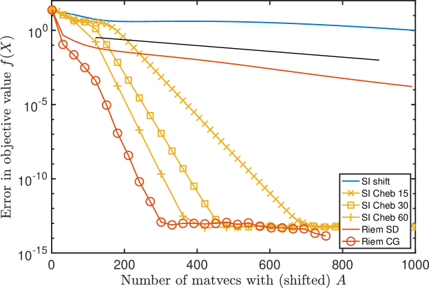
Figure 4: Error in objective value for subspace iteration (SI) and Riemannian steepest descent (SD) and nonlinear conjugate gradients (CG) for a Laplacian matrix of size $n=1\,400$ based on finite differences when computing the dominant subspace of dimension $p=6$. For SI, optimal shift and optimal Chebyshev polynomials were used of various degree (number in legend). The black lines estimate the asymptotic convergence speed as explained in the text.

6.3 A few other matrices

As our next experiment, we apply the same algorithms from the previous section to a few different matrices and several choices for the subspace dimension $p$. In addition, we target also the minimal eigenvalues by applying the methods to $-A$ instead of $A$. Except for the standard finite difference matrices for the 3D Laplacian, the matrices used were taken from the SuiteSparse Matrix Collection [10]. This results in problems with moderately large Riemannian condition numbers $\kappa$, defined in (42).

Due to the larger size of some of these matrices, we first compute with a Krylov–Schur method (implemented in Matlab as eigs) the eigenvalues that are required to determine the optimal Chebyshev filter in subspace iteration. The Riemannian methods do not require this or any other information.

FD3D

This matrix is the 3D analogue of the matrix we tested in the previous section. It corresponds to a standard finite difference discretization of the Laplacian in a box with zero Dirichlet boundary conditions. We used $n_{x}=35,n_{y}=40,n_{z}=25$ points in the $x,y,z$ direction, resp. The resulting matrix is of size $35\,000$. Compared to the earlier experiment, we took larger subspace dimensions and also a minimization of the Rayleigh quotient. All these elements make for a more challenging problem numerically.

problem	type	dimension $p$	Riem. cond. nb.	Cheb. degree
1	min	64	$3.53\cdot 10^{4}$	100
2	max	32	$5.54\cdot 10^{3}$	100

In Fig. 5, we see that the convergence of the maximization problem is very similar to that of the 2D case. However, the more relevant case of finding the minimal eigenvalues of a Laplacian matrix turns out to be a challenge for SI with or without Chebyshev acceleration. In fact, even with a degree 100 polynomial it takes about 1000 iterations before we see any acceleration. The Riemannian methods, on the other hand, converge much faster and already from the first iterations. While the nonlinear CG iteration has some plateau, it happens at a smaller error, only lasts for 300 iterations, and it still makes meaningful progress.

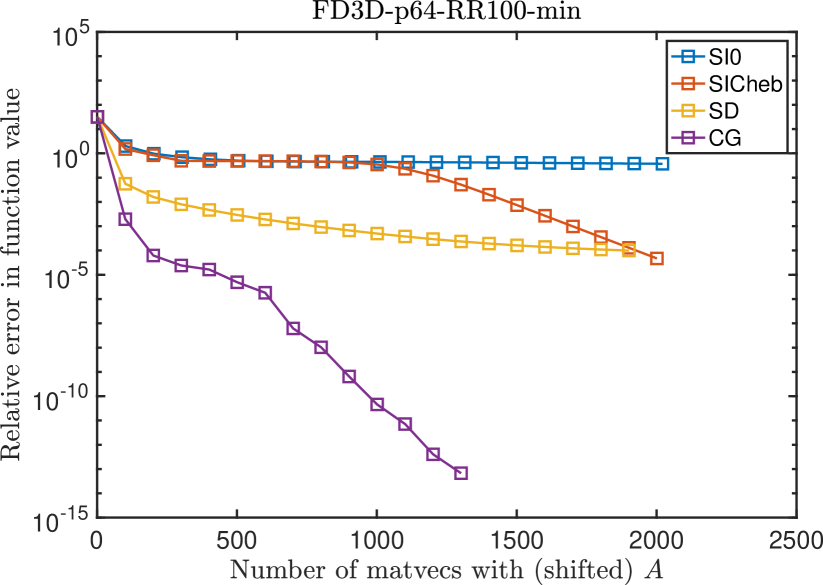
Problem nb. 1

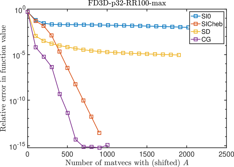
Problem nb. 2

Figure 5: The FD3D matrix.

ukerbe1

This matrix is related to a 2D finite element problem on a locally refined grid and it has a relatively small of size $n=5\,981$. It is therefore more challenging than the uniform grid of the Laplacian examples above. We tested the following parameters.

problem	type	dimension $p$	Riem. cond. nb.	Cheb. degree
3	max	32	$4.85\cdot 10^{3}$	50
4	max	64	$5.21\cdot 10^{3}$	100

In Figure 6, we observe that the Riemannian algorithms converge faster than their subspace iteration counterparts. This behavior is seen for many choices of $p$ and the Chebyshev degree. Since the spectrum of this matrix is symmetric around zero, the min problems are mathematically equivalent to the max problems, and therefore omitted.

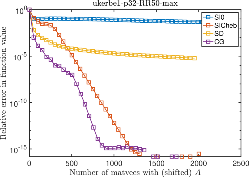
Problem nb. 3

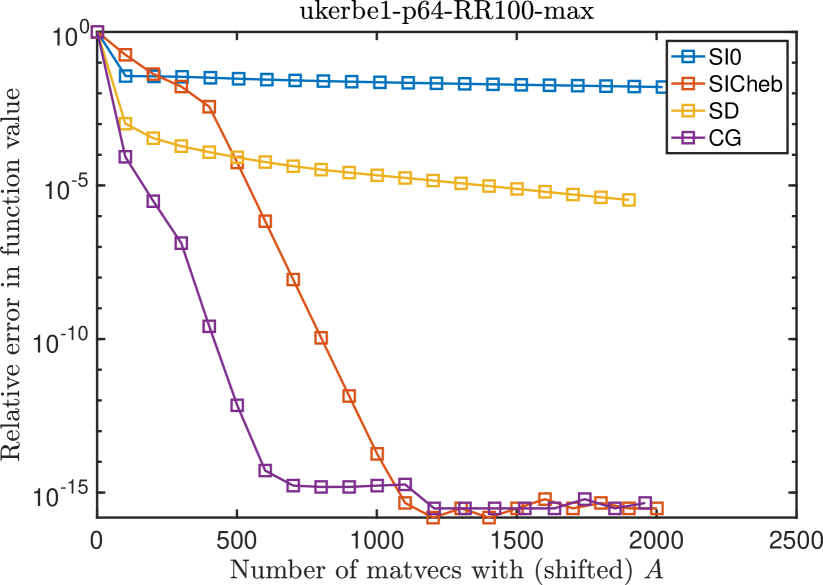
Problem nb. 4

Figure 6: The ukerbe1 matrix.

ACTIVSg70K

We now test a larger matrix of size 69 999. It models a synthetic (yet realistic) power system grid from the Texas A&M Smart Grid Center. This matrix has a spectral gap of $\mathcal{O}(10)$ but the Riemannian condition number, which represents the correct relative measure of difficulty, is still large. Such a different kind of scale makes this an interesting matrix to test our algorithms.

problem	type	dimension $p$	Riem. cond. nb.	Cheb. degree
5	min	16	$1.15\cdot 10^{4}$	50
6	max	32	$1.29\cdot 10^{3}$	50

For the minimisation problem (nb. 3), we see the Riemannian algorithms converge considerably faster than subspace iteration with or without Chebyshev acceleration of degree 50. (The reason for the bad performance of the Chebyshev acceleration is due to numerical instability with a degree 50 polynomial for this problem.) In addition, we see that Riemannian CG does not give any meaningful acceleration compared to Riemannian SD. Moreover, the linesearch has numerical issues since the error in function value increases around iterations 1000 and 1700. In theory, the error is monotonic. See section 6.4 for a more detailed analysis of this issue and an ad-hoc fix.

For the maximization problem (nb. 4), Chebyshev acceleration with degree 50 is clearly superior to Riemannian CG. However, Riemannian SD outperforms subspace iteration without acceleration. We remark that the Chebyshev acceleration needs quite accurate information on the spectrum to determine the filter polynomial, whereas the Riemannian algorithms do not require any information.

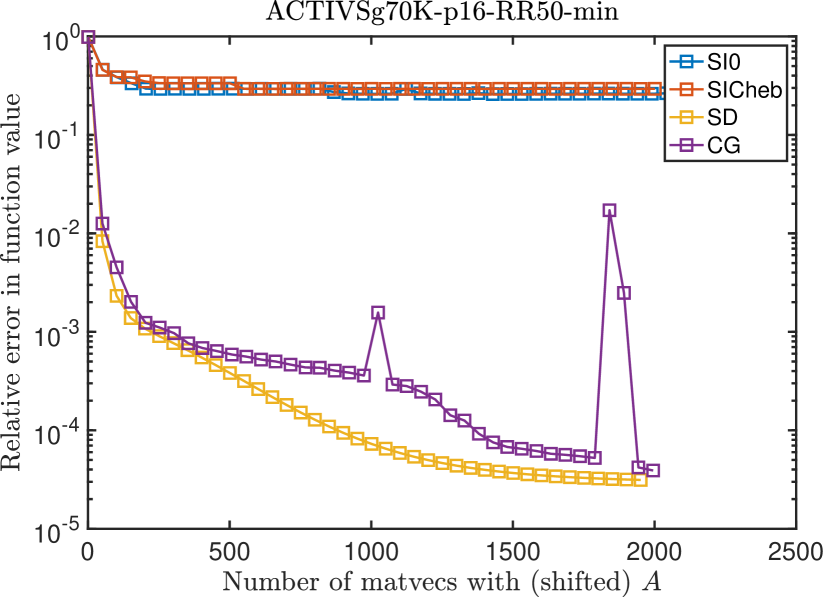
Problem nb. 5

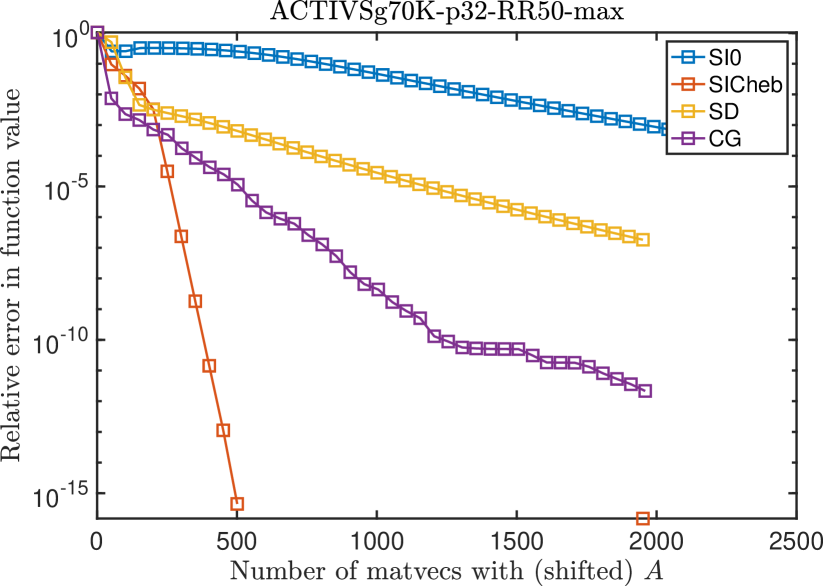
Problem nb. 6

Figure 7: The ACTIVSg70K matrix.

boneS01

This final matrix is part of the Oberwolfach model order reduction benchmark set and models a 3D trabecular bone. It is our largest example of size $n=127\,224$. As we can see from the table below, for subspace dimension $p=64$ the minimization problem is particurlay challenging with a large Riemannian condition number.

problem	type	dimension $p$	Riem. cond. nb.	Cheb. degree
7	min	64	$2.57\cdot 10^{6}$	25
8	max	64	$2.05\cdot 10^{3}$	25

The convergence of the methods is visible in Fig. 8. We can make similar observations as for the example above: for the minimization problem the Riemannian methods are superior but for the maximization the Chebyshev iteration performs the best.

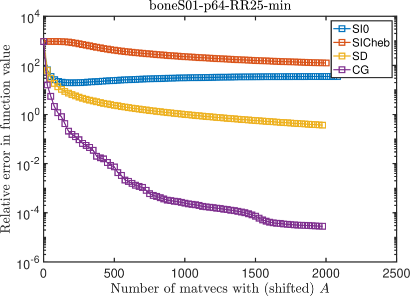
Problem nb. 7

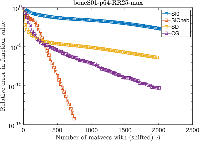
Problem nb. 8

Figure 8: The boneS01 matrix.

6.4 Numerical cancellation

As was already mentioned for the ACTIVSg70K matrix above, the line search does not always produce iterates that are monotonic in the objective function. This should be the case theoretically and thus the calculation in finite precision leads to this undesired behavior.

We conjecture that the issue is due to a catastrophic cancellation in floating point arithmetic. To support this conclusion, we repeated the same experiment as in the left panel of Fig. 7 (problem nb. 3) but now in quad precision (128 bit) compared to the standard double precision (64 bit) using the Advanpix multiprecision toolbox.

Fig. 9 compares Riemannian CG with and without multiprecision. When the calculation is done in multiprecision, the convergence is clearly smoother in function value and residual, and also monotonic in function value. An ad-hoc solution for Riemannian CG is to simply restart the iteration with the gradient if an increase of function value is detected. For this problem, the Riemannian CG in double precision then leads to a convergence plot that is similar to that in quad precision but slightly worse.

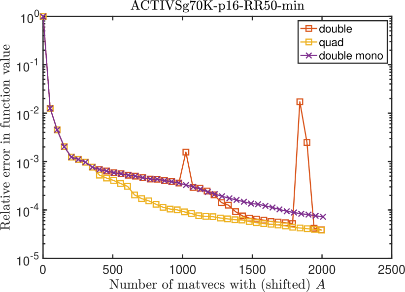
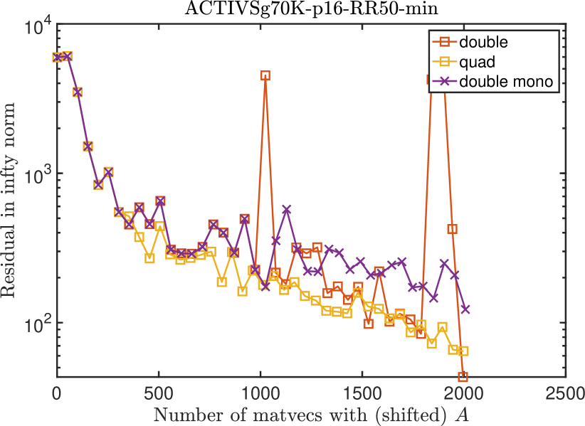
Figure 9: The ACTIVSg70K matrix calculated also in multiprecision (quad) and standard precision with enforced monotonicity (double mono).

7 Conclusion

We revisited the standard Riemannian gradient descent method for the symmetric eigenvalue problem as a more competitive alternative of subspace iteration. If accelerated using a momentum term from nonlinear CG, there is a wide variety of matrices where the Riemannian method is faster per number of matrix vector products than subspace iteration with optimal Chebyshev filter polynomials. This property would make it valuable in applications like the self-consistent field (SCF) iteration.

Among novel contributions, we derived a computationally efficient exact line search. Its accurate implementation is key to the good performance of the method. We also presented new convergence proofs for this geodesic-free Riemannian algorithm, including a locally fast convergence result in a $\mathcal{O}(\sqrt{\delta})$ neighbourhood of the dominant subspace.

References

- [1] P. A. Absil, R. Mahoney, R. Sepulchre, and P. Van Dooren, A grassmann–rayleigh quotient iteration for computing invariant subspaces, SIAM Review, 44 (2002), pp. 57–73.
- [2] P.-A. Absil, R. Mahony, and R. Sepulchre, Optimization Algorithms on Matrix Manifolds, Princeton University Press, Princeton, NJ, 2008.
- [3] K. Ahn and F. Suarez, Riemannian perspective on matrix factorization, arXiv preprint arXiv:2102.00937, (2021).
- [4] F. Alimisis, P. Davies, B. Vandereycken, and D. Alistarh, Distributed principal component analysis with limited communication, Advances in Neural Information Processing Systems, 34 (2021).
- [5] F. Alimisis and B. Vandereycken, Geodesic convexity of the symmetric eigenvalue problem and convergence of riemannian steepest descent, arXiv preprint arXiv:2209.03480, (2022).
- [6] F. L. Bauer, Das verfahren der treppeniteration und verwandte verfahren zur losung algebraischer eigenwertprobleme, ZAMP, 8 (1957), pp. 214–235.
- [7] F. Bouchard, J. Malick, and M. Congedo, Riemannian optimization and approximate joint diagonalization for blind source separation, IEEE Transactions on Signal Processing, 66 (2018), pp. 2041–2054.
- [8] F. Chatelin, Simultaneous Newton’s iteration for the eigenproblem, in Defect Correction Methods. Computing Supplementum, vol 5, S. H. Böhmer K., ed., Vienna, 1984, Springer.
- [9] P. Comon and G. H. Golub, Tracking a few extreme singular values and vectors in signal processing, Proceedings of the IEEE, 78 (1990), pp. 1327–1343.
- [10] T. A. Davis and Y. Hu, The university of florida sparse matrix collection, ACM Trans. Math. Softw., 38 (2011).
- [11] X. G. Doukopoulos and G. V. Moustakides, Fast and stable subspace tracking, Signal Processing, IEEE Transactions on, 56 (2008), pp. 1452–1465.
- [12] A. Edelman, T. A. Arias, and S. T. Smith, The geometry of algorithms with orthogonality constraints, SIAM J. Matrix Anal. Appl., 20 (1999), pp. 303–353.
- [13] L. Hoegaerts, L. D. Lathauwer, J. Suykens, and J. Vanderwalle, Efficiently updating and tracking the dominant kernel eigenspace, 16th International Symposium on Mathematical Theory of Networks and Systems, (2004). Belgium.
- [14] D. G. Luenberger and Y. Ye, Linear and Nonlinear Programming, Springer, New York, NY, 3rd edition ed., July 2008.
- [15] M. Moonen, P. Van Dooren, and J. Vandewalle, A singular value decomposition updating algorithm for subspace tracking, SIAM Journal on Matrix Analysis and Applications, 13 (1992), pp. 1015–1038.
- [16] P. O. Perry and P. J. Wolfe, Minimax rank estimation for subspace tracking, Selected Topics in Signal Processing, IEEE Journal of, 4 (2010), pp. 504–513.
- [17] H. Rutishauser, Computational aspects of F. L. Bauer’s simultaneous iteration method, 13 (1969), pp. 4–13.
- [18] , Simultaneous iteration for symmetric matrices, in Handbook for automatic computations (linear algebra), J. Wilkinson and C. Reinsch, eds., New York, 1971, Springer Verlag, pp. 202–211.
- [19] Y. Saad, J. Chelikowsky, and S. Shontz, Numerical methods for electronic structure calculations of materials, 52 (2009), pp. 3–54.
- [20] A. H. Sameh and Z. Tong, The trace minimization method for the symmetric generalized eigenvalue problem, J. Comput. Appl. Math., 123 (2000), pp. 155–175.
- [21] A. H. Sameh and J. A. Wisniewski, A trace minimization algorithm for the generalized eigenvalue problem, 19 (1982), pp. 1243–1259.
- [22] G. W. Stewart, An updating algorithm for subspace tracking, Signal Processing, IEEE Transactions on, 40 (1992), pp. 1535–1541.
- [23] S. Ubaru and Y. Saad, Fast methods for estimating the numerical rank of large matrices, in Proceedings of The 33rd International Conference on Machine Learning, M. F. Balcan and K. Q. Weinberger, eds., vol. 48 of Proceedings of Machine Learning Research, New York, New York, USA, 20–22 Jun 2016, PMLR, pp. 468–477.
- [24] Y. Zhou, J. R. Chelikowsky, and Y. Saad, Chebyshev-filtered subspace iteration method free of sparse diagonalization for solving the kohn–sham equation, Journal of Computational Physics, 274 (2014), pp. 770 – 782.
- [25] Y. Zhou, Y. Saad, M. L. Tiago, and J. R. Chelikowsky, Parallel self-consistent-field calculations via Chebyshev-filtered subspace acceleration, Phy. rev. E, 74 (2006), p. 066704.