Type I critical dynamical scalarization and descalarization in Einstein-Maxwell-scalar theory

Abstract

We investigated the critical dynamical scalarization and descalarization of black holes within the framework of the Einstein-Maxwell-scalar theory featuring higher-order coupling functions. Both the critical scalarization and descalarization displayed first-order phase transitions. When examining the nonlinear dynamics near the threshold, we always observed critical solutions that are linearly unstable static scalarized black holes. The critical dynamical scalarization and descalarization share certain similarities with the type I critical gravitational collapse. However, their initial configurations, critical solutions, and final outcomes differ significantly. To provide further insights into the dynamical results, we conducted a comparative analysis involving static solutions and perturbative analysis.

1. Department of Physics and Siyuan Laboratory, Jinan University, Guangzhou 510632, China
2. School of Physical Sciences, University of Chinese Academy of Sciences, Beijing 100049, China
3. Center for Gravitation and Cosmology, College of Physical Science and Technology, Yangzhou University, Yangzhou 225009, China
4. Institute of Theoretical Physics, Chinese Academy of Sciences, Beijing 100190, China
5. School of Physics and Optoelectronics, South China University of Technology, Guangzhou 510641, China
6. School of Aeronautics and Astronautics, Shanghai Jiao Tong University, Shanghai 200240, China

1 Introduction

The discovery of critical gravitational collapse stands as one of the most significant achievements in numerical relativity [1]. This phenomenon arises when generic initial data for collapsing matter is fine-tuned by adjusting a single parameter, denoted as $p$, to reach the critical threshold $p_{*}$ for black hole formation. Under these conditions, a unique linearly unstable critical solution (CS) emerges. Acting as an attractor, this CS serves as a boundary, distinguishing between two possible outcomes: the formation of a black hole spacetime or the preservation of a flat spacetime. Notably, the CS can exhibit characteristics of either a stationary star or a time-dependent self-similar configuration, corresponding to type I or type II critical phenomena, respectively [2]. In type II critical gravitational collapse, which occurs within a localized region, the matter and metric undergo pulsations on decreasing temporal and spatial scales until a singularity forms at the center. Near the threshold, the resulting black hole mass scales as $M\propto(p-p_{*})^{\gamma}$ in the vicinity of the threshold. The critical exponent $\gamma$ is universal, independent of the specific details of the initial data, although it does depend on the nature of the collapsing matter [3, 4, 5, 6, 7]. Type II critical gravitational collapse shares similarities with second-order phase transitions, where the order parameter, in this case, the black hole mass, exhibits continuity near the threshold. In contrast, type I critical phenomena in gravitational collapse involve the formation of a black hole with a minimum finite radius, resulting in a discontinuous transition [8, 9]. The duration of the intermediate solution, which can be approximated by the CS at the threshold, scales as $T\propto-\gamma\ln|p-p_{\ast}|$. The coefficient $\gamma$ also exhibits universality in this context. Gravitational collapse has been extensively studied in various scenarios, including complex scalar fields [10, 11, 12], Yang-Mills fields [13, 14, 15, 16], and modified gravity [17, 18, 19]. In asymptotically anti-de Sitter (AdS) spacetime, critical gravitational collapse is connected to gravitational turbulent instability [20, 21, 22].

The gravitational collapse critical phenomena arise in the transition from a flat space to a black hole. More recently, a new type of critical gravitational dynamical behavior has been discovered in the context of black hole scalarization within the framework of the Einstein-Maxwell-scalar (EMS) theory featuring higher-order coupling functions [23]. It appears during the transition from a metastable bald black hole (BBH) to a metastable scalarized black hole (SBH). Here the BBH represents the Reissner-Nordström (RN) black hole. Specifically, in the regime of critical dynamical scalarization, when the perturbation parameter $p$ approaches the threshold $p_{*}$, a CS which corresponds to a linearly unstable SBH, always emerges. The intermediate solutions persist on the CS for a duration scaling as $T\propto-\gamma\ln|p-p_{*}|$. The final solutions near the threshold exhibit a mass gap. These behaviors bear resemblance to type I critical gravitational collapse and are referred to as type I critical dynamical scalarization. However, the final masses of the resulting black holes follow power laws of the form $M_{p}-M_{\pm}\propto|p-p_{*}|^{\gamma_{\pm}}$, where $M_{\pm}$ represent the masses of the SBH and BBH, respectively, as $p$ approaches $p_{*}$ from above or below. The exponents $\gamma_{\pm}$ depend on the initial data. These power laws are absent in type I critical gravitational collapse and stem from the energy escaping to infinity. In the case of asymptotically AdS spacetime, these power laws are also absent due to energy confinement [24]. Furthermore, in our work [24], we explored the dynamical descalarization and identified two distinct types of critical behaviors in the EMS theory in asymptotically AdS spacetime. One type bears resemblance to type I critical dynamical scalarization, where a linearly unstable CS emerges. The other type is reminiscent of type II critical gravitational collapse, characterized by a scalar value $\phi_{H}$ on the apparent horizon following the relation $\phi_{H}\propto(p_{*}-p)^{1/2}$. We refer to the latter as type II critical dynamical descalarization. In a gravitational theory with scalar field coupling with both Gauss-Bonnet invariant and Ricci scalar [25], we further found a marginally stable CS in the type I critical dynamical descalarization.

In this paper, we aim to expand upon our previous work presented in [23], which exclusively focused on the critical dynamical scalarization occurring in asymptotically flat spacetime. Furthermore, our previous study maintained a fixed total mass throughout the dynamical evolution. However, this approach is somewhat unnatural as the total mass should increase with the perturbation. In this current study, we adopt a different approach by keeping the mass of the initial seed RN black hole fixed and allowing the total mass to increase with the perturbation. Through this modification, we discover the existence of a threshold for descalarization, in addition to the threshold for scalarization. Additionally, we explore the critical dynamical descalarization starting from an initial seed SBH. All of these critical dynamics fall under the category of type I. To enhance our understanding of the dynamical outcomes, we conduct a comparative analysis with the static solutions and perturbative analysis, thereby delving into the intriguing distinctions between the type I critical dynamical scalarization and type I gravitational collapse.

The organization of this paper is as follows. Section 2 provides an introduction to the EMS theory. In Section 3, we outline the numerical setups employed for the dynamical simulation of scalarization and descalarization. We provide a comprehensive description of the critical dynamics involved in these processes. Section 4 delves into the static solutions and quasinormal modes, enabling a comparison with the dynamical results and offering valuable insights into the critical dynamics. Finally, we conclude with a summary and discussion in Section 5.

2 Einstein-Maxwell-scalar theory

The action of the EMS theory considered in this study is given by

$$S=\frac{1}{16\pi}\int d^{4}x\sqrt{-g}\left[R-2\nabla_{\mu}\phi\nabla^{\mu}\phi-f(\phi)F_{\mu\nu}F^{\mu\nu}\right],$$ (1)

where natural units are employed. Here, $R$ represents the Ricci scalar, $F_{\mu\nu}=\partial_{\mu}A_{\nu}-\partial_{\nu}A_{\mu}$ denotes the field strength of Maxwell field $A_{\mu}$, and the real scalar field $\phi$ nonminimally couples to the Maxwell invariant through the coupling function $f(\phi)$. The Einstein equations are given by

$$R_{\mu\nu}-\frac{1}{2}Rg_{\mu\nu}=2\left(T_{\mu\nu}^{\phi}+f(\phi)T_{\mu\nu}^{A}\right),$$ (2)

where the energy-momentum tensor of the scalar and Maxwell fields are expressed as

$$T_{\mu\nu}^{\phi}= \partial_{\mu}\phi\partial_{\nu}\phi-\frac{1}{2}g_{\mu\nu}\nabla_{\rho}\phi\nabla^{\rho}\phi,$$ (3)

$$T_{\mu\nu}^{A}= F_{\mu\rho}F_{\nu}^{\ \rho}-\frac{1}{4}g_{\mu\nu}F_{\rho\sigma}F^{\rho\sigma}.$$

The equation of motion for the scalar field is given by

$$\nabla_{\mu}\nabla^{\mu}\phi=\frac{1}{4}\frac{df(\phi)}{d\phi}F_{\mu\nu}F^{\mu\nu},$$ (4)

while the equations for the Maxwell field are

$$\nabla_{\mu}\left(f(\phi)F^{\mu\nu}\right)=0.$$ (5)

In this study, we primarily focus on models characterized by a coupling function of the form $f(\phi)=e^{\beta\phi^{n}}$, where $n$ is a positive integer and $\beta$ denotes the coupling parameter that quantifies the strength of the coupling. Specifically, when $n=1$, these models are commonly known as Einstein-Maxwell-dilaton theories. Such theories find relevance in low-energy string theories, supergravity models, and Kaluza-Klein models [26, 27]. From (4), it becomes evident that in models with $n=1$, RN black holes with $\phi=0$ do not constitute valid solutions, leaving only the existence of dilatonic black holes. Dilatonic black holes offer a theoretical framework for exploring the influence of new degrees of freedom on the behavior of gravitational and electromagnetic fields [28, 29, 30, 31]. Furthermore, these black holes have been extensively studied in the context of holographic models due to their intricate phase structures [32, 33, 34, 35, 36].

In recent years, the EMS models with $n=2$ have attracted much attention due to the phenomenon of spontaneous scalarization [37, 38, 39, 40, 41, 42, 43, 44, 45, 46, 47], which has the potential to serve as a probe for testing the strong-field regime of gravity and for explaining certain astrophysical observations [48, 49]. In this case, RN black holes are solutions. But they may have tachyonic instability against scalar perturbations when the coupling is strong and the charge to mass ratio of the black hole is large. To be more concrete, the scalar perturbation on the RN black hole background with a coupling function of $f(\phi)=e^{\beta\phi^{2}}$ is governed by the equation

$$\nabla_{\mu}\nabla^{\mu}\delta\phi=\mu_{\text{eff}}^{2}\delta\phi,$$ (6)

where the effective mass squared is given by $\mu_{\text{eff}}^{2}=-\frac{\beta Q^{2}}{2r^{4}}$. Here $Q$ is the electric charge of the RN black hole. For positive values of $\beta$, the scalar perturbation has a negative $\mu_{\text{eff}}^{2}$, leading to a tachyonic instability. As a result, the linearly unstable bald RN black holes will dynamically evolve into the linearly stable SBHs [50, 51, 52, 38, 37].

More recently, there has been significant interest in studying models with higher order coupling functions [53, 54, 55]. For instance, consider the case of $f(\phi)=e^{\beta\phi^{4}}$. In this model, the RN black holes are stable and free of tachyonic instabilities, but can be transformed into SBHs through a violent first-order dynamical transition induced by large scalar perturbations. At the threshold of perturbation, intriguing critical behaviors are observed [23, 24]. This paper extends the work presented in [23] by considering a scenario in which the total mass of the system increases with the amplitude of the scalar perturbation. Interestingly, beyond the threshold for scalarization, we also identify a threshold for descalarization. We present static solutions and study their dominant quasinormal modes, and compare them with those obtained from the dynamical approach.

3 Dynamical evolution

In this section, we investigate the dynamical evolution of black holes in EMS theories with the coupling function $f(\phi)=e^{\beta\phi^{4}}$. We focus on two distinct types of initial configurations: (1) commencing with a bald RN black hole and (2) initiating from a linealy stable SBH. For both scenarios, we introduce an ingoing scalar perturbation and simulate the evolution of the system. Nevertheless, it is important to note that the qualitative behaviors observed during critical dynamical scalarization and descalarization are not exclusive to these two specific types of initial configurations.

3.1 Equations for dynamical simulation

To study the full nonlinear evolution of a black hole under large perturbation in a spherically symmetric spacetime, we utilize the Painlevé-Gullstrand (PG) coordinates, where the metric takes the form

$$ds^{2}=-\left(1-\zeta^{2}\right)\alpha^{2}dt^{2}+2\zeta\alpha dtdr+dr^{2}+r^{2}(d\theta^{2}+\sin^{2}\theta d\phi^{2}).$$ (7)

Here, $\zeta$ and $\alpha$ are metric functions that depend on $(t,r)$, and the apparent horizon $r_{h}$ is located where $\zeta(t,r_{h})=1$. The PG coordinates are regular on the apparent horizon and have been used to study black hole dynamics [56, 57, 58, 59, 60, 51, 23, 31, 61, 25, 62]. For RN black hole solutions, $\alpha=1,\zeta=\sqrt{\frac{2M}{r}-\frac{Q^{2}}{r^{2}}}$ where $M$ is the total mass of the system and $Q$ the black hole charge.

We take the Maxwell field as $A_{\mu}dx^{\mu}=A(t,r)dt.$ The Maxwell equations (5) give

$$\partial_{r}\left(r^{2}f(\phi)\frac{1}{\alpha}\partial_{r}A\right)=0,\ \ \ \partial_{t}\left(r^{2}f(\phi)\frac{1}{\alpha}\partial_{r}A\right)=0.$$ (8)

These can be solved by

$$\partial_{r}A=\frac{Q\alpha}{r^{2}f(\phi)}.$$ (9)

Here $Q$ is an integration constant that interpreted as the black hole electric charge.

We introduce another two auxiliary variables

$$\Pi =\frac{1}{\alpha}\partial_{t}\phi-\zeta\Phi.$$ (10)

$$\Phi =\partial_{r}\phi,$$ (11)

The Einstein equations give

$$\partial_{r}\zeta= \frac{r}{2\zeta}\left(\Phi^{2}+\Pi^{2}\right)+\frac{Q^{2}}{2r^{3}\zeta f(\phi)}+r\Pi\Phi-\frac{\zeta}{2r},$$ (12)

$$\partial_{r}\alpha= -\frac{r\Pi\Phi\alpha}{\zeta},$$ (13)

$$\partial_{t}\zeta= \frac{r\alpha}{\zeta}\left(\Pi+\Phi\zeta\right)\left(\Pi\zeta+\Phi\right).$$ (14)

The equation of motion for the scalar field gives

$$\partial_{t}\phi =\alpha\left(\Pi+\Phi\zeta\right),$$ (15)

$$\partial_{t}\Pi =\frac{\partial_{r}\left[\left(\Pi\zeta+\Phi\right)\alpha r^{2}\right]}{r^{2}}+\frac{\alpha}{2}\frac{Q^{2}}{r^{4}f^{2}(\phi)}\frac{df(\phi)}{d\phi},$$ (16)

$$\partial_{t}\Phi =\partial_{r}\left[\alpha\left(\Pi+\Phi\zeta\right)\right].$$ (17)

We need to solve the metric functions $\alpha,\zeta$ and the scalar field functions $\phi,\Phi,\Pi$. Given the initial scalar distribution $\phi$ and $\Pi$, we can calculate the initial values of $\Phi,\zeta$ and $\alpha$ using equations (11,12,13), respectively. Armed with these initial values, we can proceed to the subsequent time slice, where we obtain the values of $\zeta,\phi,\Pi$ by employing the evolution equations (14,15,16), respectively. The values of $\Phi$ and $\alpha$ can be obtained by applying constraint equations (11,13), respectively. By repeating this iterative procedure, we can obtain all the metric and scalar functions at each time step. It is worth noting that we only need to use the constraint equation (12) once at the beginning.

3.2 Numerical setup

At large distances from the black hole, it can be demonstrated that $\zeta=\sqrt{\frac{2M}{r}}\left(1+O(1/r)\right)$, where the constant $M$ represents the total mass of the system, accounting for the energy of the gravity, Maxwell and scalar fields [63]. Note that the Arnowitt-Deser-Misner (ADM) mass in PG coordinates always evaluates to zero and does not reflect the correct physical mass of the spacetime [64]. Therefore, we employ the Misner-Sharp (MS) mass, defined as [65]

$$m(t,r)=\frac{r}{2}\left(1-g^{\mu\nu}\partial_{\mu}r\partial_{\nu}r\right)=\frac{r}{2}\zeta(t,r)^{2}.$$ (18)

It can be easily shown that the RN black hole possesses $m=M-\frac{Q^{2}}{2r}$. The MS mass can be regarded as the radially integrated energy density of the energy momentum tensor [66, 59]. On the apparent horizon $r_{h}$, we have $m(t,r_{h})=\frac{1}{2}r_{h}$, which equals to the irreducible mass $M_{h}$ of the black hole defined by $M_{h}=\sqrt{\frac{A_{h}}{16\pi}}$, where $A_{h}=4\pi r_{h}^{2}$ denotes the area of the apparent horizon. The total mass of the system can then be calculated as

$$M=\lim_{r\to\infty}m(t,r)=\lim_{r\to\infty}\frac{r}{2}\zeta(t,r)^{2}.$$ (19)

To ensure the stability and long-term evolution of the numerical simulation, we encounter challenges stemming from the decay of $\zeta$. As a remedy, we introduce a new variable $s=\sqrt{r}\zeta$ in our simulations. Additionally, the decay of $\zeta$ poses difficulties in imposing outer boundary conditions at a fixed finite $r$ [59]. To address this issue, we introduce a coordinate compactification given by

$$z=\frac{r}{1+r/L},$$ (20)

where $L=1$ represents a fixed unit length scale. The system is evolved within the region $z\in[z_{c},1)$, where $z=1$ corresponds to the spatial infinity. Here $z_{c}=\frac{r_{c}}{1+r_{c}}$, with $r_{c}$ denoting a cutoff located close to the initial apparent horizon $r_{h}$ from the interior. Consequently, we evolve the system within the region $r\in[r_{c},\infty)$. It should be noted that since the radius of apparent horizon never decreases in EMS theory, $r_{c}$ always remains inside the apparent horizon throughout the entire evolution. We discretize $z$ uniformly using $2^{12}$ grid points. The resolution is limited in the far region during late times, but this does not affect our analysis as our focus is on the near horizon behavior. We employ the finite difference method in the radial direction and the fourth-order Runge-Kutta method in the time direction. To stabilize the numerical simulation, we utilize the Kreiss-Oliger dissipation. In the first step, we apply the Newton-Raphson method to solve the constraint equation (12), where the L’Hospital’s rule is used at $z=1$.

We have checked the accuracy and convergence of our numerical method by various ways. The convergence of finite difference method is often estimated by $\frac{u_{2N}-u_{N}}{u_{4N}-u_{2N}}=2^{n}+O(\frac{1}{N})$ in which $u_{N}$ is the results by using $N$ grid points, $n$ is the accurate order. It turns out that our numerical solutions converge indeed to fourth order [31, 23, 25]. Furthermore, we have also employed the second-order finite difference method to simulate the evolution and the results are qualitatively consistent.

3.2.1 Initial conditions

We take two distinct types of initial configuration:

(1) The seed black hole is a BBH with $M_{0}=1,Q=0.9.$ It has metric function $\zeta_{0}(r)=\sqrt{\frac{2M_{0}}{r}-\frac{Q^{2}}{r^{2}}}$ and scalar distribution $\phi_{0}(r)=0$. The initial apparent horizon locates at $r_{h}=1.436$ or $z_{h}=0.5895$. We take an ingoing initial scalar perturbation with the form

$$\delta\phi(r)= p\begin{cases}10^{-2}e^{-\frac{1}{r-r_{1}}-\frac{1}{r_{2}-r}}(r_{2}-r)^{2}(r-r_{1})^{2},&r_{1}<r<r_{2},\\ 0,&\text{otherwise},\end{cases}$$ (21)

$$\Pi(r)= \partial_{r}\delta\phi(r).$$

in which $r_{1}=4,r_{2}=9$ and $p$ is the perturbation amplitude parameter.

(2) The seed black hole is an SBH with $M_{0}=1.2,Q=0.9$ and the scalar charge $Q_{s}=0.6939$. It is obtained by solving the static equations of motion directly, as will be described in detail in subsection 4.1. We still refer to the metric function of the seed black hole as $\zeta_{0}(r)$ and nontrivial scalar distribution as $\phi_{0}(r)$. The initial apparent horizon is located at $r_{h}=2.149$ or $z_{h}=0.6824$. We introduce an ingoing scalar perturbation with the form

$$\delta\phi(r)= p\begin{cases}10^{-2}e^{-\frac{1}{r-r_{1}}-\frac{1}{r_{2}-r}}(r_{2}-r)^{2}(r-r_{1})^{2},&r_{1}<r<r_{2},\\ 0,&\text{otherwise},\end{cases}$$ (22)

$$\Pi(r)= \partial_{r}\delta\phi(r)-\zeta_{0}(r)\partial_{r}\phi_{0}(r).$$

in which $r_{1}=6,r_{2}=10$ and $p$ is the perturbation amplitude parameter.

3.2.2 Boundary conditions

We specify following boundary condition for (13) to solve $\alpha$ in the evolution:

$$\alpha|_{r\to\infty}=1,$$ (23)

This choice of boundary condition stems from the auxiliary freedom of $\alpha dt$ in PG coordinates and implies that an observer at infinity will measure time using the proper time coordinate $t$. We also requre that

$$\phi|_{r\to\infty}=0,\ \ \ \Pi|_{r\to\infty}=0,\ \ \ \Phi|_{r\to\infty}=0,$$ (24)

during the evolution. They imply that $\partial_{t}\phi|_{r\to\infty}=\partial_{t}\Pi|_{r\to\infty}=0$ in (15,16). These conditions are sensible as matter cannot reach spatial infinity in a finite amount of time.

As previously mentioned, we use (12) to solve for the initial values of $\zeta$ or $s$. For this purpose, we specify the following boundary condition:

$$\zeta|_{t=0,r=r_{c}}=\zeta_{0}(r_{c}).$$ (25)

Here $\zeta_{0}(r)$ refers to the metric function of the initial seed BBH or SBH, as described in the preceding subsection. This boundary condition is reasonable since the initial perturbation affects only the geometry in $r>r_{2}$ in both cases, while the geometry in $r\leq r_{1}$ remains unchanged by the perturbation at the initial time. This aspect will be explicitly demonstrated in Fig.1 and Fig.8. After obtaining the initial $\zeta$ or $s$ using (12), we can calculate the total mass of the system via (19). During subsequent evolution, we fix

$$s|_{r\to\infty}=\sqrt{2M}.$$ (26)

This specification implies that we set $\partial_{t}s|_{r\to\infty}=0$ in (14) during the evolution.

3.3 Dynamical results when the seed black hole is a RN black hole

We fix the coupling parameter $\beta=2000$ and the black hole chagre $Q=0.9$ in this subsection. The seed black hole is a BBH with a total mass $M=1$. After applying the ingoing scalar field perturbation (21), the spacetime transforms into a nonequilibrium state and the dynamical evolution commences. In Fig.1, we present the early evolution of the scalar field and MS mass. The scalar perturbation propagates inwards, and drives the evolution of the seed black hole. As implied by the right panel, in the beginning, the spacetime geometry remains unchanged in the region $r<r_{1}$, resembling that of the seed RN black hole. However, in the region $r>r_{2}$, the geometry resembles that of a larger RN black hole with a larger total mass, where the increase in mass arises from the perturbation of the scalar field.

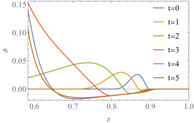
Figure 1: The early evolution of the scalar field and MS mass when the seed black hole is a bald RN black hole with a total mass $M=1$. In the right panel, the dashed blue curve represents the MS mass for the seed RN black hole. The solid blue curve with $t=0$ represents the MS mass of a nonequilibrium spacetime when the ingoing perturbation (21) with amplitude $p=0.1462$ is applied. The total mass increases to $M=1.049$.

Within the family of initial data (21) parametrized by $p$, we observe the presence of two distinct thresholds: $p_{1}\approx 0.1461857045705$ and $p_{2}\approx 0.2789936530457$. It is worth noting that while the last few digits of these threshold values may be influenced by numerical specifics, the first few digits remain consistent. When $p$ is below $p_{1}$, the final black hole remains a BBH. Conversely, when $p$ lies between $p_{1}$ and $p_{2}$, the final black hole undergoes scalarization and becomes an SBH. Interestingly, for $p$ exceeding $p_{2}$, the final black hole reverts to being a BBH once again. As such, we refer to $p_{1}$ and $p_{2}$ as the thresholds for dynamical scalarization and descalarization, respectively.

3.3.1 Dynamical critical behaviors of scalarization

Let us consider the dynamics for scalarization near $p_{1}$ at first. We monitor the evolution of the scalar value $\phi_{h}$ on the apparent horizon and the black hole irreducible mass $M_{h}$. The results are depicted in Fig.2. From the left panel, we see that $\phi_{h}$ evolves from zero. As $p$ approaches $p_{1}$ from either below or above, after experiencing a rapid change in the early stages of evolution, all the intermediate solutions are attracted to a plateau. The closer $p$ is to $p_{1}$, the longer $\phi_{h}$ remains on this plateau. Essentially, the plateau represents a linearly unstable static CS. By precisely fine-tuning $p$ to the exact threshold $p_{1}$, the evolution would hypothetically remain indefinitely on the CS. However, at late times, the evolution of $\phi_{h}$ deviates from the CS. As long as $p<p_{1}$, the final black hole remains bald, while if $p>p_{1}$, the black hole undergoes scalarization, acquiring a nonvanishing scalar field and transforming into an SBH. We use the term subcritical to describe the case where $p<p_{1}$, critical to describe the case where $p=p_{1}$, and supercritical to describe the case where $p>p_{1}$.

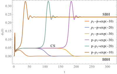
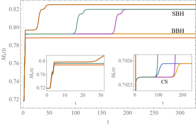
Figure 2: The evolution of the scalar field on the apparent horizon $\phi_{h}$ and the black hole irreducible mass $M_{h}$ with various $p$ near $p_{1}\approx 0.1461857045705$ for initial data family (21). The irreducible mass of the CS is very close to that of the final BBH. Their differences are shown in the right inset in the right panel. The left inset shows the evolution of $M_{h}$ in the early times.

The phenomenon of a plateau is also observed in the right panel of Fig.2. The duration of $M_{h}$ staying on this plateau becomes longer as $p$ approaches $p_{1}$. It is worth noting that the irreducible mass of the black hole never decreases during the evolution, which aligns with the expectation based on the second law of black hole thermodynamics. In the subcritical case, the final BBH has a irreducible mass very close to that of the CS. In the supercritical case, the final SBH has a much larger irreducible mass than the CS.

In summary, the evolution process for $p$ near threshold $p_{1}$ can be summerized as follows:

$$\text{BBH (metastable) }+\text{perturbation}\to\begin{cases}\text{BBH (metastable)},&\text{subcritical }(p<p_{1}),\\ \text{CS (unstable SBH)},&\text{critical }(p=p_{1}),\\ \text{SBH (metastable)},&\text{supercritical }(p_{1}<p<p_{2}).\end{cases}$$ (27)

The initial seed RN black hole behaves as a lineary stable BBH under small scalar field perturbation. However, when the perturbation becomes sufficiently strong, scalarization occurs and the BBH transitions into a linearly stable SBH. At the precise threshold, a CS arises, which represents a linearly unstable SBH and acts as an attractor.

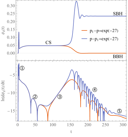
Figure 3: The evolution of $\phi_{h}$ and $\ln|\frac{d\phi_{h}}{dt}|$ when $p-p_{1}=\pm e^{-27}$ for initial data (21).

To provide a more detailed analysis of the dynamical process, we present the evolution of $\ln|\frac{d\phi_{h}}{dt}|$ in Fig.3. Regardless of whether the case is subcritical or supercritical, the entire evolution can be divided into five distinct stages. In the first stage, the incoming scalar field perturbation is captured by the seed black hole, resulting in a sudden increase in the irreducible mass of the black hole, as depicted in the right panel of Fig.2. The scalar value $\phi_{h}$ on the apparent horizon also undergoes drastic changes. The second and third stages, as shown in Fig.3, correspond to the plateau. In both subcritical and supercritical cases, the intermediate solution converges to the CS with a damping rate $\nu_{1}\approx 0.14$ in the second stage, while subsequently departing exponentially from the CS with an exponent $\eta_{1}\approx 0.136$ in the third stage. The fourth and fifth stage can be interpreted as the quasinormal modes (QNMs) and late time tail of the final black hole, respectively, under small perturbation. The dominant mode can be extracted by using the Prony method [67]. For the supercritical case, the dominant mode exhibits a complex frequency $\omega_{1s}\approx 0.532-0.126i$, while for the subcritical case, the dominant mode has a frequency $\omega_{1b}\approx 0.115-0.099i$.

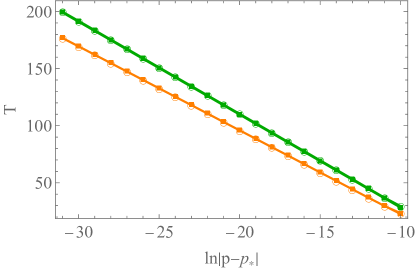
Figure 4: The time $T$ of the intermediate solution remains on the CS with respect to $\ln|p-p_{*}|$ for initial data (21). Here $p_{*}$ represents thresholds $p_{1}$ or $p_{2}$. The orange circles and squares are results for subcritical and supercritical cases near $p_{1}$, respectively. The green circles and squares are results for subcritical and supercritical cases near $p_{2}$, respectively.

The duration $T$ for which the intermediate solution remains on the CS can be estimated by observing the time when $\ln|\frac{d\phi_{h}}{dt}|$ reaches its maximum after the first stage. This maximum occurs at the turning point between the third and fourth stages. For values of $p$ that are close to $p_{1}$, we have found

$$T\propto-\gamma_{1}\ln|p-p_{1}|,$$ (28)

where $\gamma_{1}=\frac{1}{\eta_{1}}\approx 7.36$. This relationship is explicitly shown in Fig.4. It suggests that the intermediate solution in the second and third stages can be approximated as

$$\phi_{p_{1}}(t,r)=\phi_{*1}(r)+(p-p_{1})e^{\eta_{1}t}\delta\phi_{1}(r)+\text{stable modes.}$$ (29)

Here $\phi_{*1}(r)$ represents the CS at the exact threshold $p_{1}$, and $\eta_{1}$ is the eigenvalue associated with the single unstable eigenmode $\delta\phi_{1}(r)$. The stable modes dominates the evolution during the second stage. In the third stage, the unstable mode $\delta\phi_{1}(r)$ starts to dominate as its coefficient grows to a finite size, namely, $|p-p_{1}|e^{\eta_{1}T}\sim O(1)$ which implies (28). When $t\approx T$, the unstable mode grows to the same order as $\phi_{*1}(r)$. The backreaction of the unstable modes on the spacetime destroys the CS, and leads to the transition of the CS into a linearly stable BBH with a vanishing scalar field when $p<p_{1}$, or a linearly stable SBH with a nonvanishing scalar field when $p>p_{1}$. It is worth noting that the approximation (29) bears resemblance to the one found in type I critical gravitational collapse [3, 5, 9]. It has been also found in sGB theory [25] and some holographic models [68, 69, 70].

We have also investigated the evolution of $\ln\frac{dM_{h}}{dt}$, and discovered an intriguing relationship that holds throughout most of the dynamic process:

$$\ln\frac{dM_{h}}{dt}=2\ln\left|\frac{d\phi_{h}}{dt}\right|+\text{const}.$$ (30)

This relation remains valid for various initial amplitudes $p$ and system parameters like $M_{0},Q,\beta$. Note that the black hole irreducible mass never decreases, so there is no need to take the absolute value of $\frac{dM_{h}}{dt}$ in (30). This relation can be understood through perturbative analysis of static background solutions. Suppose $\alpha_{0}(r),\zeta_{0}(r)$ are background metric functions, and $\Pi_{0}(r),\Phi_{0}(r),\phi_{0}(r)$ are background scalar field functions. As we have mentioned before (19), the irreducible mass is equal to half of the black hole horizon areal radius $r_{h}$. Using the fact that the apparent horizon is located where $\zeta(t,r_{h})=1$, its evolution can be expressed as

$$\frac{dM_{h}}{dt}=\frac{1}{2}\frac{dr_{h}}{dt}=-\frac{1}{2}\left.\frac{\partial_{t}\zeta}{\partial_{r}\zeta}\right|_{r=r_{h}},$$ (31)

For static solutions, we have $\left.\zeta_{0}\right|_{r=r_{h}}=1$. On the horizon, (14) gives $\left.\Pi_{0}+\Phi_{0}\right|_{r=r_{h}}=0$. Then the leading order of (10) gives

$$\left.\delta\Pi\right|_{r=r_{h}}=\left.\frac{1}{\alpha_{0}}\partial_{t}\delta\phi-\delta\Phi\right|_{r=r_{h}}.$$ (32)

Here $\delta\Pi,\delta\Phi,\delta\phi$ represent perturbations on the static background. The leading order of (14) gives

$$\left.\partial_{t}\delta\zeta\right|_{r=r_{h}}=\left.r\alpha_{0}\left(\delta\Pi+\delta\Phi\right)^{2}\right|_{r=r_{h}}=\frac{r_{h}}{\alpha_{h}}\left.(\partial_{t}\delta\phi)^{2}\right|_{r=r_{h}},$$ (33)

where $\alpha_{h}=\alpha_{0}(r_{h})$. By combining the expansion (53) and temperature (57) for static solutions, we obtain

$$\frac{dM_{h}}{dt}=\frac{r_{h}^{2}}{\alpha_{h}}\left(1-\frac{Q^{2}}{f(\phi_{h})r_{h}^{2}}\right)^{-1}\left.(\partial_{t}\delta\phi)^{2}\right|_{r=r_{h}}=\frac{r_{h}}{4\pi T_{h}}\left.(\partial_{t}\delta\phi)^{2}\right|_{r=r_{h}}.$$ (34)

Taking the logarithm of the equation, we arrive at equation (30). The const term in (30) is equal to $\ln\frac{r_{h}}{4\pi T_{h}}$. It differs between the CS and the final black hole with or without a scalar field (BBH or SBH). This relationship emphasizes that the second and third stages can be viewed as perturbations on the CS, while the fourth and fifth stages can be seen as perturbations on the final BBH or SBH. It represents an enhanced version of the similar relationships found in other EMS models [50, 34, 31, 23]. But this relation may not hold in other theory, for example, the sGB theory [61, 25].

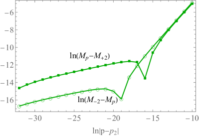
Figure 5: The power law between the irreducible masses of the final black holes and the amplitude $p$ for initial data (21). The orange circles and squares are results for subcritical and supercritical cases near $p_{1}$, respectively. The green circles and squares are results for subcritical and supercritical cases near $p_{2}$, respectively.

Furthermore, in the late stages, when the system reaches equilibrium, we observe the emergence of power laws that relate the irreducible mass of the final black hole to the initial perturbation amplitude $p$. Specifically, we find

$$M_{-1}-M_{p}\propto(p_{1}-p){}^{\gamma_{-1}},\ \ \ M_{p}-M_{+1}\propto(p-p_{1})^{\gamma_{+1}},$$ (35)

for subcritical and supercritical cases, respectively. Here $M_{p}$ and $M_{\pm 1}$ are the irreducible masses of the final black holes resulting from the initial data (21) with amplitude $p$ and $p_{\pm 1}\to p_{1}$ from above and below, respectively. As depicted in the left panel of Fig.5, for values $\ln|p-p_{1}|\lesssim-20$, the indices $\gamma_{\pm 1}\approx 0.21$. The values of $\gamma_{\pm 1}$ are not universal and depend on the families of initial data and system parameters, such as $M_{0},Q,\beta$ [23]. However, we consistently observe the power laws (35) in all cases of the critical dynamical transition. These fractional indices are absent in type I critical gravitational collapse. It is noteworthy that when $p$ deviates significantly from $p_{1}$, the indices $\gamma_{\pm 1}\approx 1$. We propose that the fractional power laws arise due to the matter escaping to spatial infinity during the evolution. Indeed, we did not find fractional indices in asymptotic AdS spacetime, where all matter remains confined, resulting in indices always equal to 1 [24].

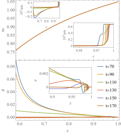
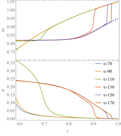
Figure 6: The snapshots of the scalar field and MS mass distribution at mid-late times. The left and right panels depict the cases with initial amplitude $p=p_{1}-e^{-20}$ (subcritical) and $p=p_{1}+e^{-20}$ (supercritical), respectively. The total mass of the system is $M=1.04873$. The evolution of the scalar values $\phi_{h}$ on the apparent horizon is illustrated in Fig.2. In the left panel, the insets present snapshots of $\Delta m=m_{RN}-m$, where $m_{RN}$ is the MS mass of the final bald RN black hole with a total mass of $M=1.04806$. In the right panel, the final SBH possesses a total mass of $M=0.949646$, as indicated by the dashed blue curve.

Finally, let us examine the evolution of the scalar field and the MS mass distribution of the gravitational system at mid to late times. This process corresponds to either the removal or the growth of the scalar field of the intermediate CS for the subcritical or supercritical cases, respectively. The snapshots of this evolution are depicted in Fig.6. In the subcritical case, the scalar field of the intermediate CS is absorbed by the central black hole, resulting in the formation of a bald RN black hole. Only a small fraction of energy (approximately $0.064\%$) escapes to spatial infinity. However, the situation is quite different for the supercritical case. The scalar field outside the black hole grows, leading to the formation of a SBH. The energy of the scalar field comes from the Maxwell field. At late times, around $9.45\%$ of the energy escapes to spatial infinity.

3.3.2 Dynamical critical behaviors of descalarization

Now we delve into the dynamics for descalarization near the threshold $p_{2}$. As depicted in Fig.7, we observe similar dynamical critical behaviors. When $p<p_{2}$, the final outcome is an SBH, whereas for $p>p_{2}$, it transforms into a bald RN black hole. At the precise threshold $p_{2}$, a linearly unstable static CS emerges. The closer $p$ is to $p_{2}$, the longer the intermediate solutions remains on this CS. The scalar values $\phi_{h}$ on the horizon of the intermediate CS and final SBH are almost the same with those obtained for amplitudes near $p_{1}$. However, given the more perturbation energy, here the irreducible mass $M_{h}$ of the intermediate CS, final BBH and SBH are all significantly larger compared to those obtained near $p_{1}$. It is worth noting that the final BBHs still possess a smaller irreducible mass compared to the SBH near $p_{2}$. In summary, the dynamical evolution process for $p$ near threshold $p_{2}$ can be succinctly summarized as follows:

$$\text{BBH (metastable) }+\text{perturbation}\to\begin{cases}\text{SBH (metastable)},&\text{subcritical }(p_{1}<p<p_{2}),\\ \text{CS (unstable SBH)},&\text{critical }(p=p_{2}),\\ \text{bald BH (metastable)},&\text{supercritical }(p>p_{2}).\end{cases}$$ (36)

Figure 7: The evolution of the scalar field value $\phi_{h}$ on the apparent horizon and the black hole irreducible mass $M_{h}$ with respect to various $p$ near threshold $p_{2}\approx 0.2789936530457$ for initial data family (21). The insets in the right panel show the evolution of $M_{h}$ in the early and middle times. The irreducible mass of the CS is very close to that of the final BBH.

By analyzing the evolution of $\ln|\frac{d\phi_{h}}{dt}|$, we observe similar patterns as depicted in Fig.3. The evolution still can be divided into five distinct stages. Following a violent change in the first stage, the intermediate solution gradually approaches the CS in the second stage, exhibiting a damping rate of $\nu_{2}\approx 0.14$. In the third stage, the solution departs from the CS exponentially, with an exponent of $\eta_{2}\approx 0.123$. During the fourth stage, the solution converges towards the final SBHin the subcritical case, characterized by a dominant mode $\omega_{2s}\approx 0.432-0.116i$. Conversely, in the supercritical case, the solution evolves towards the final BBH with a dominant mode $\omega_{2b}\approx 0.098-0.090i$.

The duration $T$ for which intermediate solution remains on the CS still satisfies a similar relation in the form of (28), as shown in Fig.4. The new coefficient $\gamma_{2}=\frac{1}{\eta_{2}}\approx 8.14$. Moreover, as shown in the right panel of Fig.5, we observe that the relations (35) still hold. When $p$ is very close to $p_{2}$, and the corresponding coefficients $\gamma_{\pm 2}\approx 0.21$. For $p$ that deviates significantly from $p_{2}$, the coefficients $\gamma_{\pm 2}\approx 1$.

3.4 Dynamical results when the seed black hole is a scalarized black hole

In this subsection, we investigate the cases when the seed black hole takes the form of an SBH with a total mass of $M=1.2$. The coupling parameter $\beta=2000$ and the black hole chagre $Q=0.9$ remain fixed. The seed SBH exhibits a nontrivial distribution of the background scalar field, characterized by a scalar charge of $Q_{s}=0.6939$. To initiate the evolution, we apply an ingoing scalar field perturbation using the expression (22). Fig.8 presents the early evolution of the scalar field and the MS mass. As depicted by the right panel, initially, the spacetime geometry remains unchanged in the region $r<r_{1}$, resembling that of the seed SBH. However, beyond the region $r>r_{2}$, the geometry undergoes a transformation into a novel state that is distinct from both SBH and RN black hole. The scalar perturbation propagates inward, driving the evolution of the spacetime.

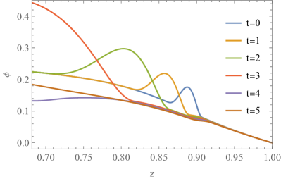
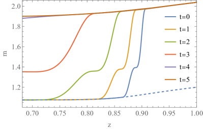
Figure 8: The early evolution of the scalar field and MS mass when the seed black hole is an SBH with a total mass $M=1.2$. In the right panel, the dashed blue curve represents the MS mass for the seed SBH. The solid blue curve with $t=0$ represents the MS mass of a nonequilibrium spacetime when the ingoing perturbation (22) with amplitude $p=0.1285$ is applied. The total mass increases to $M=2.038$.

Unlike the cases described in subsection 3.3, for the initial data (22) parametrized by $p$, we find only one threshold $p_{3}\approx 0.1284877802279$. The final black hole keeps scalarized when $p<p_{3}$. However, it undergoes descalarization and becomes a bald RN black hole when $p>p_{3}$. Near the threshold, we still observe type I critical dynamical behaviors. The evolution of the scalar field value $\phi_{h}$ on the apparent horizon and black hole irreducible mass $M_{h}$ when $p$ is close to $p_{3}$ are depicted in Fig.9. Note that the initia value of $\phi_{h}$ is nonzero here. When the ingoing scalar perturbation reaches the black hole horizon, the system experiences a drastic change. The scalar field increases fast and then drops fast. The black hole irreducible mass increases a lot from $1.0745$ to $1.9224$. Then the intermediate solution is attracted to a CS, and remains on the CS for a duration satisfying $T\propto-\gamma_{3}\ln|p-p_{3}|$, in which $\gamma_{3}=21.08$. At last, the intermediate solution departs the CS exponentially with exponent $\eta_{3}=\frac{1}{\gamma_{3}}\approx 0.0475$. It converges to a final SBH when $p<p_{3}$ or to a final RN black hole when $p>p_{3}$.

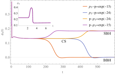
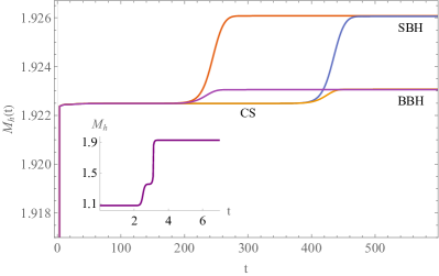
Figure 9: The evolution of the scalar field value $\phi_{h}$ on the apparent horizon and the black hole irreducible mass $M_{h}$ with respect to various $p$ near threshold $p_{3}\approx 0.1284877802279$ for initial data family (22). The insets show the evolution of $\phi_{h}$ and $M_{h}$ in the early times.

We have found similar critical dynamical behaviors when the seed SBH has a total mass of $M=1.8$ or $2$, where a linearly unstable CS always emerges on the descalarization threshold. In summary, the critical dynamics near $p_{3}$ for descalarization of an SBH can be expressed as follow:

$$\text{SBH (metastable) }+\text{perturbation}\to\begin{cases}\text{SBH (metastable)},&\text{subcritical }(p<p_{3}),\\ \text{CS (unstable SBH)},&\text{critical }(p=p_{3}),\\ \text{bald BH (metastable)},&\text{supercritical }(p>p_{3}).\end{cases}$$ (37)

3.5 Comparison with type I critical gravitational collapse

The critical dynamical scalarization and descalarization we have describled above resemble the type I critical gravitational collapse, which can be summarized as follows:

$$\text{flat space (metastable)}+\text{perturbation}\to\begin{cases}\text{flat space (metastable)},&\text{subcritical }(p<p_{\ast}),\\ \text{CS (unstable star)},&\text{critical }(p=p_{\ast}),\\ \text{BH (stable)},&\text{supercritical }(p>p_{\ast}).\end{cases}$$ (38)

Here the initial state is a flat spacetime. When the matter perturbation is small, the matter will dissipates and leave a flat spacetime. But when the perturbation is large, a black hole will be formed. At the threshold, a CS emerges. The CS is a linearly unstable star. The duration $T$ for which the intermediate solution remains on the CS still obey a relation $T\propto-\gamma\ln|p-p_{*}|$. Here the coefficient $\gamma$ is a universal constant, regardless of the initial data family. This is different from the critical dynamical scalarization and descalarization here, in which the coefficient $\gamma$ is related to the initial data family [23]. The source of this difference comes from the fact that there is only one CS in the type I critical gravitational collapse, but many CSs in the critical dynamical scalarization and descalarization. This will be demonstrated in the next section.

4 Static solutions and quasinormal modes

In the previous section, we discovered the crucial role of CSs in the critical dynamics near the threshold. These CSs are, in fact, statically linearly unstable SBHs, while the final SBH and BBH are static linearly stable solutions. In this section, we solve the static equations of motion directly, and delve into the thermodynamic property and perturbative stability of the CS, final SBH and BBH.

4.1 Equations of motion for static solutions and their perturbations

To investigate the static solutions and their perturbative properties in a spherical context, we adopt the following metric ansatz:

$$ds^{2}=-\tilde{N}e^{-2\tilde{\delta}}dt_{s}^{2}+\frac{1}{\tilde{N}}dr^{2}+r^{2}(d\theta^{2}+\sin^{2}\theta d\phi^{2}).$$ (39)

Here, the metric functions $\tilde{N}$ and $\tilde{\delta}$ depend on $t,r$ and take the following forms:

$$\tilde{N}(t,r)=N(r)+\epsilon N_{1}(r)e^{-i\omega t},\ \ \ \tilde{\delta}(t,r)=\delta(r)+\epsilon\delta_{1}(r)e^{-i\omega t}.$$ (40)

The scalar field is assumed to be

$$\tilde{\phi}(t,r)=\phi(r)+\epsilon\phi_{1}(r)e^{-i\omega t}.$$ (41)

The Maxwell field is determined by $\partial_{r}A=\frac{Qe^{-\tilde{\delta}}}{r^{2}f(\tilde{\phi})}$ where $Q$ represents the electric charge of the black hole. Here, $N,\delta$, and $\phi$ are background metric and scalar functions for the static solutions, $\epsilon$ is the control parameter in the linear expansion, and the complex quantity $\omega=\omega_{R}+i\omega_{I}$ corresponds to the quasinormal modes or eigenvalues of the perturbative eigenstates $N_{1},\delta_{1}$, and $\phi_{1}$. By substituting these ansatz into the equations of motion for gravity and scalar fields, and expanding the equations with respect to $\epsilon$, we obtain the following leading-order equations.

$$\partial_{r}N =\frac{1-N}{r}-r(\partial_{r}\phi)^{2}N-\frac{Q^{2}}{r^{3}f(\text{$\phi$})},$$

$$\partial_{r}\delta =-r(\partial_{r}\phi)^{2},$$ (42)

$$\partial_{r}^{2}\phi =\frac{1}{rN}\left(N+1-\frac{Q^{2}}{r^{2}f(\phi)}\right)\partial_{r}\phi+\frac{Q^{2}}{2r^{4}Nf^{2}(\phi)}\frac{df(\phi)}{d\phi}.$$

At the subleading order, we find that the metric perturbations can be expressed in terms of scalar field perturbation as

$$N_{1}= -2rN\phi_{1}\partial_{r}\phi,\ \ \ \partial_{r}\delta_{1}=-2r\partial_{r}\phi\partial_{r}\phi_{1}.$$ (43)

Then the equation for scalar field perturbation is decoupled from the metric perturbations and can be reduced to a Schrödinger-like equation:

$$\left(\frac{d^{2}}{dr_{*}^{2}}+\omega^{2}-V_{\text{eff}}\right)\psi=0.$$ (44)

Here we have introduced the tortoise coordinate $r_{*}$ by $\frac{dr_{*}}{dr}=\frac{1}{Ne^{-\delta}}$, and defined $\psi(r)=r\phi_{1}(r)$. The effective potential [38]

$$V_{\text{eff}}= \frac{Ne^{-2\delta}}{r^{2}}\left[1-N-2r^{2}\phi^{\prime}{}^{2}-\frac{Q^{2}}{r^{2}f}\left(1-2r^{2}\phi^{\prime}{}^{2}+\frac{2r\phi^{\prime}\dot{f}}{f}+\frac{f\ddot{f}-2\dot{f}{}^{2}}{2f^{2}}\right)\right],$$ (45)

where $\phi^{\prime}=\partial_{r}\phi,$ $\dot{f}=\frac{df(\phi)}{d\phi}$, and $\ddot{f}=\frac{d^{2}f(\phi)}{d\phi^{2}}$.

We can solve the static background metric and scalar functions using equations (42), and then substitute them into equations (44,45) to determine the quasinormal mode $\omega$ under appropriate boundary conditions. However, in order to directly compare the results obtained from the dynamical approach, we perform a coordinate transformation

$$dt_{s}=dt-\frac{\zeta}{(1-\zeta^{2})\alpha}dr,$$ (46)

to convert to the PG coordinates (7). This transformation is feasible when the background are time-independent. The metric functions are related as

$$N=1-\zeta^{2},\ \ \ e^{-\delta}=\alpha.$$ (47)

For static background solutions, the equations of motion (42) turn to be

$$0= \partial_{r}\alpha-r\alpha(\partial_{r}\phi)^{2},$$ (48)

$$0= \partial_{r}\zeta+\frac{\zeta}{2r}-\frac{r(1-\zeta^{2})}{2\zeta}(\partial_{r}\phi)^{2}-\frac{Q^{2}}{2r^{3}\zeta f(\phi)},$$ (49)

$$0= \partial_{r}^{2}\phi+\frac{1}{\left(\zeta{}^{2}-1\right)}\left[\left(\frac{Q^{2}}{r^{2}f(\phi)}+\zeta{}^{2}-2\right)\frac{\partial_{r}\phi}{r}-\frac{Q^{2}}{2r^{4}f^{2}(\phi)}\frac{df(\phi)}{d\phi}\right].$$ (50)

The scalar perturbation equation (44) can be rewritten as

$$\left[(1-\zeta^{2})\alpha\frac{\partial}{\partial r}\left((1-\zeta^{2})\alpha\frac{\partial}{\partial r}\right)+\omega^{2}-V_{\text{eff}}\right]\psi =0,$$ (51)

where the variables $N,\delta$ in effective potential $V_{\text{eff}}$ should be replaced by (47).

4.2 Static solutions

In this subsection, our focus is on finding the solutions for the static background. It is worth noting that the equations (49,50) are decoupled from (48). This decoupling allows us to initially solve for $\zeta,\phi$ using (49,50) at first, and subsequently determine $\alpha$ using (48). To solve the static equations (49,50), it is essential to specify appropriate boundary conditions.

4.2.1 Boundary conditions and numerical setup

At spatial infinity, the solutions can be expanded as

$$\zeta= \sqrt{\frac{2M}{r}}\left(1-\frac{Q^{2}+Q_{s}^{2}}{4Mr}+\cdots\right),$$ (52)

$$\phi= \frac{Q_{s}}{r}+\frac{MQ_{s}}{r^{2}}+\cdots.$$

Here $M$ denotes the total mass of the system, and $Q,Q_{s}$ denotes the electric and scalar charge, respectively. Near the event horizon $r_{H}$ of the black hole, the solutions can be expanded as

$$\zeta= 1+\frac{1}{2r_{H}}\left(\frac{Q^{2}}{f(\phi_{H})r_{H}^{2}}-1\right)(r-r_{H})+\cdots,$$ (53)

$$\phi= \phi_{H}+\frac{Q^{2}}{2r_{H}f(\phi_{H})\left[Q^{2}-r_{H}^{2}f(\phi_{H})\right]}\frac{df(\phi_{H})}{d\phi}(r-r_{H})+\cdots,$$ (54)

where $\phi_{H}$ is the scalar value on the event horizon. Note that in EMS theory, the scalar hair is a secondary hair [71]. Given $\beta,Q$ and $M$, the scalar charge $Q_{s}$ or $\phi_{H}$ is determined.

By providing values for $\beta,Q,r_{H}$, and an initial guess value for $\phi_{H}$, and imposing the boundary conditions (53,54) at $r_{b1}=r_{H}(1+\epsilon)$, typically with $\epsilon\approx 10^{-7}$, we can numerically integrate the equations (49,50) up to $r_{b2}$ which is typically around $10^{6}r_{H}$. A static background solution is found if the solution $\phi(r)$ approaches zero at $r_{b2}$. If the solution $\phi(r)$ does not approach zero at $r_{b2}$, we need to adjust the initial guess value $\phi_{H}$ and repeat the integration process. Once we obtain static background solutions $\zeta,\phi$, we can use equation (52) to calculate the total mass $M$ and scalar charge $Q_{s}$, given by

$$M=\lim_{r\to\infty}\frac{r}{2}\zeta(r)^{2},\ \ \ Q_{s}=-\lim_{r\to\infty}r^{2}\partial_{r}\phi(r).$$ (55)

At spatial infinity, $\alpha$ can be expanded as

$$\alpha =\alpha_{0}\left(1-\frac{Q_{s}^{2}}{2r^{2}}+\cdots\right),$$ (56)

where $\alpha_{0}$ is an undetermined constant due to the auxiliary freedom in $\alpha dt$ in PG coordinate. In order to be consistent with the dynamical method, we set $\alpha_{0}=1$. The equation (48) can be solved by using above boundary expansion at $r_{b2}$. Now we can determine the black hole temperature

$$T_{H}=\frac{N^{\prime}(r_{H})}{4\pi}e^{-\delta(r_{H})}=\frac{\zeta^{\prime}(r_{H})}{2\pi}\alpha(r_{H})=\frac{\alpha(r_{H})}{4\pi r_{H}}\left(1-\frac{Q^{2}}{f(\phi_{H})r_{H}^{2}}\right).$$ (57)

The temperature of a RN black hole is given by $T_{H}=\frac{1}{4\pi r_{H}}\left(1-\frac{Q^{2}}{r_{H}^{2}}\right).$ To facilitate our analysis, we will utilize the reduced temperature $t_{H}=8\pi MT_{H}$ and the reduced entropy $s_{H}=\frac{S}{4\pi M^{2}}$, where the black hole entropy is denoted by $S=\frac{A_{H}}{4}=\pi r_{H}^{2}.$

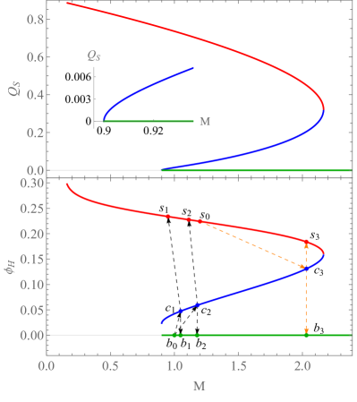
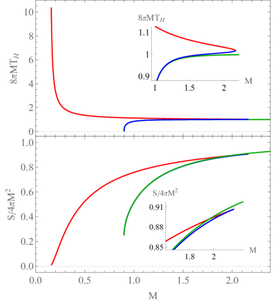
Figure 10: The scalar charge $Q_{s}$, scalar value $\phi_{H}$ on the event horizon, reduced temperature $t_{H}$, and reduced entropy $s_{H}$ are illustrated for static solutions with $\beta=2000$ and $Q=0.9$. At the same total mass $M$, we observe two branches of SBHs. The blue and red curves correspond to SBHs with lower and higher temperatures, respectively. The green curve represents the BBH. The cold SBHs exhibit temperatures and entropies that closely resemble those of the BBH. The differences between them are highlighted in the insets.

4.2.2 The results for static solutions

In Fig.10, we present various properties of static solutions, including the scalar charge $Q_{s}$, scalar value $\phi_{H}$ on the event horizon, the reduced temperature $t_{H}$, and reduced entropy $s_{H}$. These solutions are obtained with $\beta=2000$ and $Q=0.9$. We observe the presence of a bald RN black hole whenever the total mass $M$ exceeds the charge $Q=0.9$. Additionally, we identify two distinct branches of SBH solutions. The blue branch corresponds to cold SBHs characterized by lower temperatures, while the red branch represents hot SBH with higher temperatures. These branches intersect at $(M,Q_{s},\phi_{H})=(2.165,0.3214,0.1594)$. It appears that the cold branch bifurcates from the extremal RN black hole. However, the situation near the extremal black hole is highly intricate, and for a more comprehensive understanding, we refer readers to [55]. Within the range of $M\in(0.9,2.165)$, the cold SBHs, hot SBHs, and BBHs coexist. In this region, the cold SBHs always possess the smallest entropy, making them thermodynamically unfavorable. As for the hot SBHs, their entropy are either greater or smaller than those of the BBH, depending on whether $M$ lies in the range $(0.9,1.964)$ or $(1.964,2.165)$.

4.2.3 Comparison with dynamical results

When comparing with the dynamical outcomes, we observe that the critical dynamical scalarization and descalarization near the thresholds, initiated from the initial perturbation (21) applied to the seed bald RN black hole, correspond to the following trajectories:

$$b_{0}\to c_{1}\to\begin{cases}b_{1},&(p<p_{1}),\\ c_{1},&(p=p_{1}),\\ s_{1},&(p_{1}<p<p_{2}),\end{cases}\ \ \ b_{0}\to c_{2}\to\begin{cases}s_{2},&(p_{1}<p<p_{2}),\\ c_{2},&(p=p_{2}),\\ b_{2},&(p>p_{2}).\end{cases}$$ (58)

The critical dynamical descalarization, initiated from the seed SBH through the initial perturbation (22), follows the following trajectory:

$$s_{0}\to c_{3}\to\begin{cases}s_{3},&(p<p_{3}),\\ c_{3},&(p=p_{3}),\\ b_{3},&(p>p_{3}).\end{cases}$$ (59)

The characteristics of these static solutions are presented in table 1. Concerning the final equilibrium states, both scalarization and descalarization can be interpreted as first-order phase transitions, given that all the quantities exhibit a gap in the vicinity of the threshold.

	$b_{0}$	$c_{1}$	$b_{1}$	$s_{1}$	$c_{2}$	$s_{2}$	$b_{2}$	$s_{0}$	$c_{3}$	$s_{3}$	$b_{3}$
$M$	1	1.0485	1.0480	0.9496	1.1799	1.1121	1.1772	1.2	2.0320	2.0305	2.0311
$Q_{s}$	0	0.0200	0	0.7454	0.0348	0.7125	0	0.6938	0.2050	0.4503	0
$\phi_{H}$	0	0.0474	0	0.2338	0.0592	0.2276	0	0.2242	0.1310	0.1839	0
$t_{H}$	0.5851	0.8971	0.6882	1.1377	0.9553	1.1080	0.8969	1.0956	1.0079	1.0296	1.7197
$s_{H}$	0.5154	0.5713	0.5718	0.7447	0.6757	0.7845	0.6762	0.8019	0.8952	0.8969	0.8992

Table 1: The total mass $M$, scalar charge $Q_{s}$, scalar value $\phi_{H}$ on the event horizon, reduced temperature $t_{H}$, and reduced entropy $s_{H}$ for the bald RN black holes $b_{0,1,2}$, critical solutions or cold SBHs $c_{1,2,3}$, and hot SBHs $s_{0,1,2,3}$.

From table 1, we observe that the intermediate CS consistently possesses a larger total mass than the corresponding final SBH or BBH, as a result of energy escaping to spatial infinity. Additionally, the intermediate CS exhibits a smaller entropy compared to the corresponding final SBH or BBH, in accordance with the second law of black hole thermodynamics. Interestingly, the dynamics do not precisely align with thermodynamic expectations. For instance, the bald RN black hole has a smaller entropy than the hot SBH when $M\in(0.9,1.964)$. However, when the seed black hole is an RN black hole with $M=1$, subjected to perturbation (21) with amplitude $p_{1}<p<p_{2}$, the final equilibrium states of the dynamic evolution are the hot SBH with smaller entropy, rather than the RN black hole with larger entropy, as depicted in the lower left panel of Fig.10.

We compare our findings with those obtained in a generalized scalar-tensor theory, as presented in a previous study [25]. In that work, the dynamical scalarization and descalarization were investigated within a framework where the scalar field couples to both the Gauss-Bonnet curvature and the Ricci curvature. We observe that the critical dynamical scalarization exhibits typically type I behaviors to what we have found here. However, the critical dynamical descalarization displays intriguing differences. In study [25], the descalarization manifests as a first-order phase transition, from a thermodynamic standpoint. However, the phase transition point occurs at the junction where the hot and cold branches of SBH merge. In contrast, within the EMS theory presented here, the phase transition point always precedes the junction point. It will be worth exploring whether there are deeper physical reasons for this difference.

4.3 Perturbation and QNM

Now we turn to solve the perturbative equation (44) or (51), in which the effective potential is given by (45) and (47). To calculate the QNMs, we should impose ingoing boundary condition near the event horizon and outgoing boundary condition near the spatial infinity. From (41) and (44), this implies the scalar perturbation has asymptotical behaviors as follow:

$$\psi\propto\begin{cases}e^{-i\omega r_{*}}\to(r-r_{h})^{\frac{i\omega r_{h}}{\left(\frac{Q^{2}}{f(\phi_{h})r_{h}^{2}}-1\right)\alpha(r_{h})}},&r_{*}\to-\infty\ (r\to r_{h}),\\ e^{i\omega r_{*}}\to e^{i\omega r}r^{2iM\omega},&r_{*}\to\infty\ (r\to\infty).\end{cases}$$ (60)

Here we have used the tortoise coordinate $\frac{dr_{*}}{dr}=\frac{1}{(1-\zeta^{2})\alpha}$, and its asymptotical behaviors

$$r_{*}\to\begin{cases}\frac{-r_{h}}{\left(\frac{Q^{2}}{f(\phi_{h})r_{h}^{2}}-1\right)\alpha(r_{h})}\ln(r-r_{h}),&r\to r_{h},\\ r+2M\ln r,&r\to\infty.\end{cases}$$ (61)

4.3.1 Direct integration method for unstable modes

For an unstable mode $\omega=\omega_{R}+i\omega_{I}$ with positive imaginary part, it is easy to see that

$$\psi\to\begin{cases}A_{+}e^{-(i\omega_{R}-\omega_{I})r_{*}}\to 0,&r_{*}\to-\infty\ (r\to r_{h}),\\ A_{+}e^{(i\omega_{R}-\omega_{I})r_{*}}\to 0,&r_{*}\to\infty\ (r\to\infty).\end{cases}$$ (62)

We adopt a scheme that has been previously used to calculate the unstable mode [72, 53, 25]. We introduce a squared frequency variable, $w=\omega^{2}$, and treat it as an auxiliary function, $w(r)$, which satisfies $\frac{dw}{dr}=0$. We solve this equation along with (51). The three boundary conditions are $\psi|_{r=r_{h}}=\psi|_{r=\infty}=0$, and $\psi|_{r_{m}}=1$, where $r_{m}$ is typically about $6r_{h}$. In practice, we set the inner boundary at $r=r_{h}(1+10^{-6})$ and outer boundary at $r=200r_{h}$. By following this procedure, we can successfully obtain the unstable modes. However, this procedure is not suitable for calculating stable modes with a negative imaginary part.

4.3.2 The first-order WKB method for stable modes

To calculate the stable modes, we employ the first-order WKB method [73, 74]. Using the perturbation equation (44), the quasinormal modes are determined by the equation

$$0=\omega^{2}-V_{\text{eff}}(r_{m})+\left(\frac{1}{2}+n\right)i\sqrt{-2\frac{\partial^{2}V_{\text{eff}}(r_{m})}{\partial r_{*}^{2}}},\ \ \ n=0,1,2,...$$ (63)

where $r_{m}$ corresponds to the location where $V_{\text{eff}}(r)$ reaches its maximum, $n$ represents the overtones, and $\frac{\partial}{\partial r_{*}}=(1-\zeta^{2})\alpha\frac{\partial}{\partial r}$. We primarily focus on the dominant mode with $n=0$. Once we obtain the static background solutions, we can solve above equation to determine the dominant mode. However, it should be noted that the WKB method is only applicable to stable modes [75].

4.3.3 Shooting method for QNMs

In addition to the two perturbative methods we have discussed, we will also utilize the shooting method to calculate the QNMs. Unlike the previous methods, the shooting method is applicable for both unstable and stable QNMs. To apply the shooting method, we first expand all the background functions around the black hole horizon using a high-order expansion with a parameter denoted as $n_{b}$, typically set to around 12. The expansions are given by:

$$h=\sum_{n=0}^{n_{b}}h_{n}(r-r_{H})^{n}.$$ (64)

where $h$ represents the variables $\zeta,\alpha,\phi$. By utilizing the background equations (48-50) and providing numerical values for $\beta,Q$, and $r_{H}$, we can efficiently determine the coefficients $h_{n}$ order by order. Next, we expand all the background functions near spatial infinity as follows:

$$\phi=\sum_{n=1}^{n_{b}}\frac{\phi_{n}}{r^{n}},\ \ \ \zeta=\sqrt{\frac{2M}{r}}\sum_{n=0}^{n_{b}}\frac{\zeta_{n}}{r^{n}},\ \ \ \alpha=\sum_{n=0}^{n_{b}}\frac{\alpha_{n}}{r^{n}},$$ (65)

where $\phi_{0}=Q_{s},\zeta_{0}=1$, and $\alpha_{0}=1$ to be coincident with (52,56). We can also efficiently obtain the coefficients $\phi_{n},\zeta_{n},\alpha_{n}$ order by order.

Now let us consider the perturbation field $\psi$. Near the black hole horizon and spatial infinity, we respectively assume the ingoing and outgoing asymptotic behavior in the form:

$$\psi_{-}(r)=e^{-i\omega r_{*}}Y(r),\ \ \ \psi_{+}(r)=e^{i\omega r_{*}}Z(r),$$ (66)

where $Y$ and $Z$ are regular functions near the horizon and infinity, respectively. By substituting (66) into (51), after dropping the factor $e^{\pm i\omega r_{*}}$, we obtain a linear differential equation for $Y$ and $Z$, respectively. We expand $Y$ around the horizon and $Z$ near infinity with an order denoted as $n_{p}$, typically chosen to be smaller than $n_{b}$:

$$Y=\sum_{n=0}^{n_{p}}Y_{n}(r-r_{H})^{n},\ \ \ Z=\sum_{n=0}^{n_{p}}Z_{n}r^{-n}.$$ (67)

where we take $n_{p}=8$. Substituting (67) into the linear differential equation for $Y$ and $Z$, and combining the results with static background expansion coefficients (64) and (65), we can efficiently determine $Y_{n}$ and $Z_{n}$ order by order, respectively. These coefficients depend on $\omega$. Providing an initial guess value of $\omega$, we obtain $Y(r)$ by integrating the linear differential equation for $Y$ from the inner boundary at $r_{b1}=r_{H}(1+10^{-3})$ to the midpoint $r_{m}\sim 5r_{H}$ for the boundary conditions $Y(r_{b1}),Y^{\prime}(r_{b1})$. With the same initial guess value of $\omega$, we obtain $Z(r)$ by integrating the linear differential equation for $Z$ from the outer boundary at $r_{b2}\sim 100r_{H}$ to the midpoint $r_{m}$ for the boundary conditions $Z(r_{b2}),Z^{\prime}(r_{b2})$. At the midpoint $r_{m}$, we require $\psi_{-}(r_{m})=\psi_{+}(r_{m})$ and $\frac{d\psi_{-}}{dr}(r_{m})=\frac{d\psi_{+}}{dr}(r_{m})$, which leads to the condition:

$$\left.\frac{1}{Y}\frac{dY}{dr}-\frac{1}{Z}\frac{dZ}{dr}-2i\omega\frac{dr_{*}}{dr}\right|_{r=r_{m}}=0.$$ (68)

If above equation is not satisfied, we need to adjust the initial guess value $\omega$ and repeat the integration process. Due to the limitation of numerical accuracy, we mainly calculate the dominant modes of the static background solutions.

4.3.4 The QNMs for unstable and stable solutions

In Fig.11, we present the profiles of the effective potential for the critical solutions $c_{1,2,3}$, bald RN black holes $b_{1,2,3}$ and hot SBHs $s_{1,2,3}$. The BBHs and hot SBHs exhibit potential barriers near the horizon, whereas the CSs display potential wells in proximity to the horizon. The hot SBHs also possess potential wells, albeit situated away from the horizon. As the total mass increases, both the potential barrier and well diminish in size.

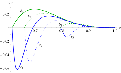
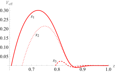
Figure 11: The profiles of the effective potential of the static solutions. The blue, green and red curves correspond to the cold SBH $c_{1,2,3}$, RN black hole $b_{1,2,3}$ (left), and hot SBH $s_{1,2,3}$ (right), respectively.

According to a well known result in quantum mechanics [76], for a perturbation equation in the form of (44), the effective potential must satisfy the condition $\int_{-\infty}^{\infty}V_{\text{eff}}dr_{*}=\int_{r_{H}}^{\infty}\frac{V_{\text{eff}}}{(1-\zeta^{2})\alpha}dr<0$ to induce instability. We have verified that only the CSs fulfill this condition, indicating their linear instability. Consequently, the CSs decay either into BBHs or hot SBHs. As previously mentioned, the CSs essentially represent cold SBHs. When they decay into BBHs, most of their scalar hair is absorbed by the central black hole, with only a small amount of energy escaping to infinity. On the other hand, when the CSs decay into SBHs, a portion of the energy from the Maxwell field is converted into scalar hair. Some of this energy dissipates into infinity, while the remainder is absorbed by the central black hole, causing significant growth of black hole irreducible mass and eventual stabilization as a linearly stable hot SBH. This stabilization is made possible by the existence of an effective potential well outside the effective potential barrier.

	$c_{1}$	$b_{1}$	$s_{1}$	$c_{2}$	$s_{2}$	$b_{2}$
Direct	$0.132i$			$0.119i$
WKB		$0.191-0.093i$	$0.561-0.119i$		$0.477-0.115i$	$0.169-0.084i$
Shooting	$0.136i$	$0.125-0.098i$	$0.548-0.129i$	$0.123i$	$0.460-0.126i$	$0.106-0.089i$
Dynamics	$0.136i$	$0.115-0.099i$	$0.532-0.126i$	$0.123i$	$0.432-0.116i$	$0.098-0.090i$

Table 2: The dominant modes for the bald RN black holes $b_{1,2}$, critical solutions or cold SBHs $c_{1,2}$, and hot SBHs $s_{1,2}$, obtained using four different methods. The direct integration method captures only the unstable modes, while the WKB method provides the stable modes exclusively. The dynamical results are extracted by using Prony method.

Table 2 provides the dominant modes of the CSs $c_{1,2}$, the final BBHs $b_{1,2}$ and the final hot SBHs $s_{1,2}$. The results for $c_{3},b_{3}$ and $s_{3}$ exhibit similar qualitative features. Four different methods were employed to obtain these modes, and the results are consistent within the acceptable error range. It is noteworthy that both the BBHs and hot SBHs consistently display complex modes with negative imaginary parts. Conversely, the CSs consistently possess purely positive imaginary eigenvalues. This observation bears resemblance to the tachyonic instability exhibited by the scalar perturbation in the context of spontaneous scalarization models [77]. Indeed, unlike superradiant instability [78, 79, 80], the existence of an effective potential well near the CS horizon implies a negative effective mass squared for scalar perturbations, indicating the possibility of tachyonic instability in the CS [81, 42, 51].

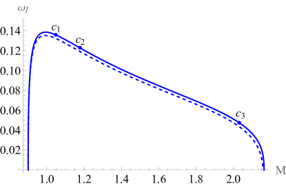
Figure 12: The unstable modes of the cold SBHs. The solid curve represents the results obtained using the shooting method, while the dashed curve corresponds to the direct integration method. The unstable modes of the critical solutions $c_{1,2,3}$ are indicated for comparison.

Considering the pivotal role of the CSs in the critical dynamical transition, which are essentially the cold SBHs, we present the dominant modes of all the cold SBHs in Fig.12. These modes are obtained using two different methods. The cold SBH branch exhibits an unstable mode characterized by $\omega_{R}=0$ and $\omega_{I}>0$ across its entire range of existence. At the two endpoints of the cold SBH branch, the value of $\omega_{I}$ approaches zero. However, it attains a maximum value at a specific $M$. We recommend referring to [54] for a more comprehensive examination of the QNMs of hot, cold and bald black holes in a similar EMS model.

5 Summary and Discussion

The EMS models offer a fascinating theoretical framework for exploring the intricate relationship between bald and hairy black holes. A classification of these models based on the black hole solutions characterized by the coupling function $f(\phi)$ was proposed in [39]. Class I models exclusively accommodate hairy black hole solutions, such as the Einstein-Maxwell-dilaton model. On the other hand, Class IIA and IIB models allow for both RN solutions and scalarized solutions. In Class IIA models, the scalarized branch is smoothly connected to the RN branch, and it may exhibit tachyonic instability, resulting in spontaneous scalarization. The model investigated in this paper belongs to Class IIB, where three distinct solution branches coexist within certain parameter ranges. Specifically, the RN and hot scalarized branches are linearly stable, while the cold scalarized branch is linearly unstable [54]. Notably, the hot scalarized branch is not continuously connected to the RN branch. The phenomenon of three branch coexistence in black hole solutions has also been observed in scalar-Gauss-Bonnet theories [82, 83, 84, 85, 86, 25, 87]. It is important to highlight that the static or perturbative analysis is insufficient to determine the nonlinear dynamics. In our previous works [23, 24, 25], we first revealed the intriguing dynamical transitions among these three solution branches. We discovered a novel physical mechanism involving nonlinear accretion that leads to black hole scalarization beyond spontaneous scalarization.

In this paper, we begin with the linearly stable bald RN black hole as the initial black hole. Only when this seed black hole accretes a sufficient amount of scalar perturbation does it undergo a transformation into a hot SBH. Interestingly, we observe the emergence of a linearly unstable CS precisely at the scalarization threshold. It is worth noting that if the perturbation is excessively strong, the final solution reverts back to being a RN black hole once again. In the context of nonlinear dynamical evolution, a similar linearly unstable CS persists at the threshold. From the perspective of static solutions, this behavior is qualitatively reasonable. When the total mass of the system is large and the charge is fixed, only RN solutions exist, while scalarized solutions only emerge when the total mass of the system is small. Additionally, we also consider the linearly stable hot SBH as the initial black hole. In this case, descalarization occurs when the scalar perturbation reaches a significant magnitude. Similarly, we observe the appearance of a linearly unstable CS at the descalarization threshold. We have analyzed effective potentials of the perturbation for all the CSs, and conclude that the CSs suffer tachyonic instability, just as the RN black holes suffer tachyonic instability under small scalar perturbation in the class IIA models. So the nonlinear scalarization of the bald black holes are induced by the tachyonic instability of the CSs. These results are not specific to our chosen initial configurations, but rather exhibit a qualitatively universal nature. We have further investigated other coupling functions belonging to Class IIB, such as $f(\phi)=e^{\beta\phi^{n}}$ or $1+\beta\phi^{n}$ when $n\geq 3$, and consistently observed qualitatively similar critical dynamical behaviors at the scalarization and descalarization thresholds.

The critical behaviors observed in dynamical scalarization and descalarization at the thresholds bear resemblance to the type I critical gravitational collapse. When the perturbation parameter $p$ approaches the threshold $p_{*}$, all intermediate solutions are attracted to a linearly unstable CS and remain on this CS for a duration described by $T\propto-\gamma\ln|p-p_{*}|$. Here the coefficient $\gamma$ equals the reciprocal of the eigenvalue of the single unstable mode associated with the CS. In type I critical gravitational collapse, the CS is unique, resulting in a universal $\gamma$ value that applies to all families of initial data. However, in the case of type I dynamical scalarization and descalarization, the CSs are not unique. Specifically, the CS belongs to the cold SBH branch, which exists within a certain parameter range. Consequently, for different initial data families, the intermediate solutions will be attacted to different CSs, leading to varying values of the corresponding coefficient $\gamma$. Furthermore, we discover that the irreducible masses of the final black holes in critical dynamical scalarization and descalarization follow power laws with fractional indices, a characteristic absent in type I critical gravitational collapse. These indices also depend on the initial data family. We propose that these fractional power laws arise due to the energy of matter escaping to infinity. However, a more comprehensive investigation is necessary to delve into this matter in the future.

The type I critical dynamcial scalarization and descalarization have been studied in the EMS theories [23, 24] as well as in a generalized scalar-tensor theory [25]. Interestingly, it appears that dynamical descalarization consistently occurs before the junction point where the cold SBH and hot SBH branches meet in EMS theories. However, in the context of the generalized scalar-tensor theory, dynamical descalarization consistently takes place precisely at the junction point. The underlying cause for this discrepancy remains unknown at present. We speculate that this distinction could be attributed to the coupling between either the gravitational curvature invariant or the matter invariant. To confirm this conjecture, further investigations regarding type I critical dynamics of black holes in other models are necessary.

Finally, let us explore some potential extensions of this work. The type I critical dynamical behaviors we have uncovered are not limited to scalarization and descalarization phenomena alone. In our preliminary research, we have found indications that these critical dynamics also manifest in black hole transitions involving Q-hair [88, 89], and a dedicated paper on this topic is forthcoming. Moreover, when examining the phase diagram presented in Fig.10, we observe certain resemblances to those observed in higher-dimensional spacetimes for black rings and Myers-Perry black holes [90]. This prompts us to speculate the existence of a type I critical dynamical transition bridging these systems. Furthermore, there are indications that type I critical dynamics manifest in the real-time processes of phase separation and nucleation during holographic first-order phase transitions [91, 92, 93, 94, 95], which have been examined in studies such as [68, 70]. Additionally, critical dynamics should exist in the first-order phase transitions of matter within specific gravity systems, resulting in the emission of gravitational waves [96, 97, 98]. Overall, the investigation of type I critical dynamics holds immense theoretical and experimental significance across various domains. These potential extensions shed light on the far-reaching implications and broad applicability of type I critical dynamics in diverse physical phenomena.

References

- Choptuik [1993] M. W. Choptuik, Universality and scaling in gravitational collapse of a massless scalar field, Phys. Rev. Lett., 70, 9 (1993).
- Gundlach and Martin-Garcia [2007] C. Gundlach and J. M. Martin-Garcia, Critical phenomena in gravitational collapse, Living Rev. Rel., 10, 5 (2007), arXiv:0711.4620 [gr-qc].
- Evans and Coleman [1994] C. R. Evans and J. S. Coleman, Observation of critical phenomena and selfsimilarity in the gravitational collapse of radiation fluid, Phys. Rev. Lett., 72, 1782 (1994), arXiv:gr-qc/9402041.
- Abrahams and Evans [1993] A. M. Abrahams and C. R. Evans, Critical behavior and scaling in vacuum axisymmetric gravitational collapse, Phys. Rev. Lett., 70, 2980 (1993).
- Koike et al. [1995] T. Koike, T. Hara, and S. Adachi, Critical behavior in gravitational collapse of radiation fluid: A Renormalization group (linear perturbation) analysis, Phys. Rev. Lett., 74, 5170 (1995), arXiv:gr-qc/9503007.
- Gundlach [1995] C. Gundlach, The Choptuik space-time as an eigenvalue problem, Phys. Rev. Lett., 75, 3214 (1995), arXiv:gr-qc/9507054.
- Choptuik et al. [2004] M. W. Choptuik, E. W. Hirschmann, S. L. Liebling, and F. Pretorius, Critical collapse of a complex scalar field with angular momentum, Phys. Rev. Lett., 93, 131101 (2004), arXiv:gr-qc/0405101.
- Brady et al. [1997] P. R. Brady, C. M. Chambers, and S. M. C. V. Goncalves, Phases of massive scalar field collapse, Phys. Rev. D, 56, R6057 (1997), arXiv:gr-qc/9709014.
- Bizon and Chmaj [1998] P. Bizon and T. Chmaj, Critical collapse of Skyrmions, Phys. Rev. D, 58, 041501 (1998), arXiv:gr-qc/9801012.
- Seidel and Suen [1991] E. Seidel and W. M. Suen, Oscillating soliton stars, Phys. Rev. Lett., 66, 1659 (1991).
- Hawley and Choptuik [2000] S. H. Hawley and M. W. Choptuik, Boson stars driven to the brink of black hole formation, Phys. Rev. D, 62, 104024 (2000), arXiv:gr-qc/0007039.
- Zhang et al. [2016a] C.-Y. Zhang, S.-J. Zhang, D.-C. Zou, and B. Wang, Charged scalar gravitational collapse in de Sitter spacetime, Phys. Rev. D, 93, 064036 (2016a), arXiv:1512.06472 [gr-qc].
- Bartnik and Mckinnon [1988] R. Bartnik and J. Mckinnon, Particle - Like Solutions of the Einstein Yang-Mills Equations, Phys. Rev. Lett., 61, 141 (1988).
- Bizon [1990] P. Bizon, Colored black holes, Phys. Rev. Lett., 64, 2844 (1990).
- Gundlach [1997] C. Gundlach, Echoing and scaling in Einstein Yang-Mills critical collapse, Phys. Rev. D, 55, 6002 (1997), arXiv:gr-qc/9610069.
- Choptuik et al. [1996] M. W. Choptuik, T. Chmaj, and P. Bizon, Critical behavior in gravitational collapse of a Yang-Mills field, Phys. Rev. Lett., 77, 424 (1996), arXiv:gr-qc/9603051.
- Liebling and Choptuik [1996] S. L. Liebling and M. W. Choptuik, Black hole criticality in the Brans-Dicke model, Phys. Rev. Lett., 77, 1424 (1996), arXiv:gr-qc/9606057.
- van Putten [1996] M. H. P. M. van Putten, Approximate black holes for numerical relativity, Phys. Rev. D, 54, R5931 (1996), arXiv:gr-qc/9607074.
- Zhang et al. [2016b] C.-Y. Zhang, Z.-Y. Tang, and B. Wang, Gravitational collapse of massless scalar field in gravity, Phys. Rev. D, 94, 104013 (2016b), arXiv:1608.04836 [gr-qc].
- Bizon and Rostworowski [2011] P. Bizon and A. Rostworowski, On weakly turbulent instability of anti-de Sitter space, Phys. Rev. Lett., 107, 031102 (2011), arXiv:1104.3702 [gr-qc].
- Dias et al. [2012] O. J. C. Dias, G. T. Horowitz, and J. E. Santos, Gravitational Turbulent Instability of Anti-de Sitter Space, Class. Quant. Grav., 29, 194002 (2012), arXiv:1109.1825 [hep-th].
- Deppe et al. [2015] N. Deppe, A. Kolly, A. Frey, and G. Kunstatter, Stability of AdS in Einstein Gauss Bonnet Gravity, Phys. Rev. Lett., 114, 071102 (2015), arXiv:1410.1869 [hep-th].
- Zhang et al. [2022a] C.-Y. Zhang, Q. Chen, Y. Liu, W.-K. Luo, Y. Tian, and B. Wang, Critical Phenomena in Dynamical Scalarization of Charged Black Holes, Phys. Rev. Lett., 128, 161105 (2022a), arXiv:2112.07455 [gr-qc].
- Zhang et al. [2022b] C.-Y. Zhang, Q. Chen, Y. Liu, W.-K. Luo, Y. Tian, and B. Wang, Dynamical transitions in scalarization and descalarization through black hole accretion, Phys. Rev. D, 106, L061501 (2022b), arXiv:2204.09260 [gr-qc].
- Liu et al. [2022] Y. Liu, C.-Y. Zhang, Q. Chen, Z. Cao, Y. Tian, and B. Wang, The critical scalarization and descalarization of black holes in a generalized scalar-tensor theory (2022), arXiv:2208.07548.
- Gibbons and Maeda [1988] G. W. Gibbons and K.-i. Maeda, Black Holes and Membranes in Higher Dimensional Theories with Dilaton Fields, Nucl. Phys. B, 298, 741 (1988).
- Garfinkle et al. [1991] D. Garfinkle, G. T. Horowitz, and A. Strominger, Charged black holes in string theory, Phys. Rev. D, 43, 3140 (1991), [Erratum: Phys.Rev.D 45, 3888 (1992)].
- Ferrari et al. [2001] V. Ferrari, M. Pauri, and F. Piazza, Quasinormal modes of charged, dilaton black holes, Phys. Rev. D, 63, 064009 (2001), arXiv:gr-qc/0005125.
- Zhang et al. [2015] C.-Y. Zhang, S.-J. Zhang, and B. Wang, Charged scalar perturbations around Garfinkle–Horowitz–Strominger black holes, Nucl. Phys. B, 899, 37 (2015), arXiv:1501.03260.
- Blázquez-Salcedo et al. [2019] J. L. Blázquez-Salcedo, S. Kahlen, and J. Kunz, Quasinormal modes of dilatonic Reissner–Nordström black holes, Eur. Phys. J. C, 79, 1021 (2019), arXiv:1911.01943 [gr-qc].
- Zhang et al. [2022c] C.-Y. Zhang, P. Liu, Y. Liu, C. Niu, and B. Wang, Dynamical scalarization in Einstein-Maxwell-dilaton theory, Phys. Rev. D, 105, 024073 (2022c), arXiv:2111.10744 [gr-qc].
- DeWolfe et al. [2011] O. DeWolfe, S. S. Gubser, and C. Rosen, Dynamic critical phenomena at a holographic critical point, Phys. Rev. D, 84, 126014 (2011), arXiv:1108.2029 [hep-th].
- Mo and Lan [2021] J.-X. Mo and S.-Q. Lan, Dynamic phase transition of charged dilaton black holes, Chin. Phys. C, 45, 105106 (2021), arXiv:2105.00868 [gr-qc].
- Zhang et al. [2022d] C.-Y. Zhang, P. Liu, Y. Liu, C. Niu, and B. Wang, Evolution of anti–de Sitter black holes in Einstein-Maxwell-dilaton theory, Phys. Rev. D, 105, 024010 (2022d), arXiv:2104.07281 [gr-qc].
- Zhao et al. [2023] Y.-Q. Zhao, S. He, D. Hou, L. Li, and Z. Li, Phase diagram of holographic thermal dense QCD matter with rotation, JHEP, 04, 115 (2023), arXiv:2212.14662 [hep-ph].
- Cai et al. [2022] R.-G. Cai, S. He, L. Li, and Y.-X. Wang, Probing QCD critical point and induced gravitational wave by black hole physics, Phys. Rev. D, 106, L121902 (2022), arXiv:2201.02004 [hep-th].
- Herdeiro et al. [2018] C. A. R. Herdeiro, E. Radu, N. Sanchis-Gual, and J. A. Font, Spontaneous Scalarization of Charged Black Holes, Phys. Rev. Lett., 121, 101102 (2018), arXiv:1806.05190 [gr-qc].
- Fernandes et al. [2019] P. G. S. Fernandes, C. A. R. Herdeiro, A. M. Pombo, E. Radu, and N. Sanchis-Gual, Spontaneous Scalarisation of Charged Black Holes: Coupling Dependence and Dynamical Features, Class. Quant. Grav., 36, 134002 (2019), [Erratum: Class.Quant.Grav. 37, 049501 (2020)], arXiv:1902.05079 [gr-qc].
- Astefanesei et al. [2019] D. Astefanesei, C. Herdeiro, A. Pombo, and E. Radu, Einstein-Maxwell-scalar black holes: classes of solutions, dyons and extremality, JHEP, 10, 078 (2019), arXiv:1905.08304 [hep-th].
- Guo et al. [2021] G. Guo, P. Wang, H. Wu, and H. Yang, Scalarized Einstein–Maxwell-scalar black holes in anti-de Sitter spacetime, Eur. Phys. J. C, 81, 864 (2021), arXiv:2102.04015 [gr-qc].
- Myung and Zou [2019a] Y. S. Myung and D.-C. Zou, Quasinormal modes of scalarized black holes in the Einstein–Maxwell–Scalar theory, Phys. Lett. B, 790, 400 (2019a), arXiv:1812.03604 [gr-qc].
- Myung and Zou [2019b] Y. S. Myung and D.-C. Zou, Instability of Reissner–Nordström black hole in Einstein-Maxwell-scalar theory, Eur. Phys. J. C, 79, 273 (2019b), arXiv:1808.02609 [gr-qc].
- Myung and Zou [2019c] Y. S. Myung and D.-C. Zou, Stability of scalarized charged black holes in the Einstein–Maxwell–Scalar theory, Eur. Phys. J. C, 79, 641 (2019c), arXiv:1904.09864 [gr-qc].
- Lai et al. [2022a] M.-Y. Lai, Y. S. Myung, R.-H. Yue, and D.-C. Zou, Spin-charge induced spontaneous scalarization of Kerr-Newman black holes, Phys. Rev. D, 106, 084043 (2022a), arXiv:2208.11849 [gr-qc].
- Lai et al. [2022b] M.-Y. Lai, Y. S. Myung, R.-H. Yue, and D.-C. Zou, Spin-induced scalarization of Kerr-Newman black holes in Einstein-Maxwell-scalar theory, Phys. Rev. D, 106, 044045 (2022b), arXiv:2206.11587 [gr-qc].
- Wei et al. [2022] S.-W. Wei, Y.-X. Liu, and R. B. Mann, Black Hole Solutions as Topological Thermodynamic Defects, Phys. Rev. Lett., 129, 191101 (2022), arXiv:2208.01932 [gr-qc].
- Lin et al. [2023] H.-J. Lin, T. Zhu, S.-J. Zhang, and A. Wang, Parity violations induced black hole scalarizations (2023), arXiv:2305.15733 [gr-qc].
- Martin and Yokoyama [2008] J. Martin and J. Yokoyama, Generation of Large-Scale Magnetic Fields in Single-Field Inflation, JCAP, 01, 025 (2008), arXiv:0711.4307 [astro-ph].
- Maleknejad et al. [2013] A. Maleknejad, M. M. Sheikh-Jabbari, and J. Soda, Gauge Fields and Inflation, Phys. Rept., 528, 161 (2013), arXiv:1212.2921 [hep-th].
- Zhang et al. [2021] C.-Y. Zhang, P. Liu, Y. Liu, C. Niu, and B. Wang, Dynamical charged black hole spontaneous scalarization in anti–de Sitter spacetimes, Phys. Rev. D, 104, 084089 (2021), arXiv:2103.13599.
- Xiong et al. [2022] W. Xiong, P. Liu, C. Niu, C.-Y. Zhang, and B. Wang, Dynamical spontaneous scalarization in Einstein-Maxwell-scalar theory, Chin. Phys. C, 46, 095103 (2022), arXiv:2205.07538 [gr-qc].
- Luo et al. [2022] W.-K. Luo, C.-Y. Zhang, P. Liu, C. Niu, and B. Wang, Dynamical spontaneous scalarization in Einstein-Maxwell-scalar models in anti–de Sitter spacetime, Phys. Rev. D, 106, 064036 (2022), arXiv:2206.05690 [gr-qc].
- Blázquez-Salcedo et al. [2020a] J. L. Blázquez-Salcedo, C. A. R. Herdeiro, J. Kunz, A. M. Pombo, and E. Radu, Einstein-Maxwell-scalar black holes: the hot, the cold and the bald, Phys. Lett. B, 806, 135493 (2020a), arXiv:2002.00963 [gr-qc].
- Luis Blázquez-Salcedo et al. [2021] J. Luis Blázquez-Salcedo, C. A. R. Herdeiro, S. Kahlen, J. Kunz, A. M. Pombo, and E. Radu, Quasinormal modes of hot, cold and bald Einstein–Maxwell-scalar black holes, Eur. Phys. J. C, 81, 155 (2021), arXiv:2008.11744 [gr-qc].
- Blázquez-Salcedo et al. [2020b] J. L. Blázquez-Salcedo, S. Kahlen, and J. Kunz, Critical solutions of scalarized black holes, Symmetry, 12, 2057 (2020b), arXiv:2011.01326 [gr-qc].
- Ziprick and Kunstatter [2009] J. Ziprick and G. Kunstatter, Numerical study of black-hole formation in Painleve-Gullstrand coordinates, Phys. Rev. D, 79, 101503 (2009), arXiv:0812.0993 [gr-qc].
- Kanai et al. [2011] Y. Kanai, M. Siino, and A. Hosoya, Gravitational collapse in Painleve-Gullstrand coordinates, Prog. Theor. Phys., 125, 1053 (2011), arXiv:1008.0470 [gr-qc].
- Ripley [2019] J. L. Ripley, Excision and avoiding the use of boundary conditions in numerical relativity, Class. Quant. Grav., 36, 237001 (2019), arXiv:1908.04234 [gr-qc].
- Ripley and Pretorius [2020a] J. L. Ripley and F. Pretorius, Scalarized Black Hole dynamics in Einstein dilaton Gauss-Bonnet Gravity, Phys. Rev. D, 101, 044015 (2020a), arXiv:1911.11027 [gr-qc].
- Ripley and Pretorius [2020b] J. L. Ripley and F. Pretorius, Dynamics of a symmetric EdGB gravity in spherical symmetry, Class. Quant. Grav., 37, 155003 (2020b), arXiv:2005.05417 [gr-qc].
- Liu et al. [2023] Y. Liu, C.-Y. Zhang, W.-L. Qian, K. Lin, and B. Wang, Dynamic generation or removal of a scalar hair, JHEP, 01, 074 (2023), arXiv:2206.05012 [gr-qc].
- Niu et al. [2022] C. Niu, W. Xiong, P. Liu, C.-Y. Zhang, and B. Wang, Dynamical descalarization in Einstein-Maxwell-scalar theory (2022), arXiv:2209.12117 [gr-qc].
- Hayward [1996] S. A. Hayward, Gravitational energy in spherical symmetry, Phys. Rev. D, 53, 1938 (1996), arXiv:gr-qc/9408002.
- Shibata [2015] M. Shibata, Numerical Relativity (100 Years of General Relativity) (World Scientific Publishing, Singapore, 2015).
- Misner and Sharp [1964] C. W. Misner and D. H. Sharp, Relativistic equations for adiabatic, spherically symmetric gravitational collapse, Phys. Rev., 136, B571 (1964).
- Ripley and Pretorius [2019] J. L. Ripley and F. Pretorius, Gravitational collapse in Einstein dilaton-Gauss–Bonnet gravity, Class. Quant. Grav., 36, 134001 (2019), arXiv:1903.07543 [gr-qc].
- Berti et al. [2007] E. Berti, V. Cardoso, J. A. Gonzalez, and U. Sperhake, Mining information from binary black hole mergers: A Comparison of estimation methods for complex exponentials in noise, Phys. Rev. D, 75, 124017 (2007), arXiv:gr-qc/0701086.
- Chen et al. [2023a] Q. Chen, Y. Liu, Y. Tian, B. Wang, C.-Y. Zhang, and H. Zhang, Critical dynamics in holographic first-order phase transition, JHEP, 01, 056 (2023a), arXiv:2209.12789 [hep-th].
- Chen et al. [2023b] Q. Chen, Z. Ning, Y. Tian, B. Wang, and C.-Y. Zhang, Descalarization by quenching charged hairy black hole in asymptotically AdS spacetime, JHEP, 01, 062 (2023b), arXiv:2210.14539 [hep-th].
- Chen et al. [2022] Q. Chen, Y. Liu, Y. Tian, X. Wu, and H. Zhang, Quench Dynamics in Holographic First-Order Phase Transition (2022), arXiv:2211.11291 [hep-th].
- Herdeiro and Radu [2015] C. A. R. Herdeiro and E. Radu, Asymptotically flat black holes with scalar hair: a review, Int. J. Mod. Phys. D, 24, 1542014 (2015), arXiv:1504.08209 [gr-qc].
- Blázquez-Salcedo et al. [2018] J. L. Blázquez-Salcedo, D. D. Doneva, J. Kunz, and S. S. Yazadjiev, Radial perturbations of the scalarized Einstein-Gauss-Bonnet black holes, Phys. Rev. D, 98, 084011 (2018), arXiv:1805.05755 [gr-qc].
- Berti et al. [2009] E. Berti, V. Cardoso, and A. O. Starinets, Quasinormal modes of black holes and black branes, Class. Quant. Grav., 26, 163001 (2009), arXiv:0905.2975 [gr-qc].
- Konoplya and Zhidenko [2011] R. A. Konoplya and A. Zhidenko, Quasinormal modes of black holes: From astrophysics to string theory, Rev. Mod. Phys., 83, 793 (2011), arXiv:1102.4014 [gr-qc].
- Konoplya et al. [2019] R. A. Konoplya, A. Zhidenko, and A. F. Zinhailo, Higher order WKB formula for quasinormal modes and grey-body factors: recipes for quick and accurate calculations, Class. Quant. Grav., 36, 155002 (2019), arXiv:1904.10333 [gr-qc].
- Nandi and Islam [1995] K. K. Nandi and A. Islam, On the optical-mechanical analogy in general relativity, Am. J. Phys., 63, 251 (1995), arXiv:0905.4479 [gr-qc].
- Doneva et al. [2022a] D. D. Doneva, F. M. Ramazanoğlu, H. O. Silva, T. P. Sotiriou, and S. S. Yazadjiev, Scalarization (2022a), arXiv:2211.01766 [gr-qc].
- Zhang et al. [2014] C.-Y. Zhang, S.-J. Zhang, and B. Wang, Superradiant instability of Kerr-de Sitter black holes in scalar-tensor theory, JHEP, 08, 011 (2014), arXiv:1405.3811 [hep-th].
- Liu et al. [2021] P. Liu, C. Niu, and C.-Y. Zhang, Instability of regularized 4D charged Einstein-Gauss-Bonnet de-Sitter black holes, Chin. Phys. C, 45, 025104 (2021), arXiv:2004.10620 [gr-qc].
- Zhang et al. [2020] C.-Y. Zhang, S.-J. Zhang, P.-C. Li, and M. Guo, Superradiance and stability of the regularized 4D charged Einstein-Gauss-Bonnet black hole, JHEP, 08, 105 (2020), arXiv:2004.03141 [gr-qc].
- Silva et al. [2018] H. O. Silva, J. Sakstein, L. Gualtieri, T. P. Sotiriou, and E. Berti, Spontaneous scalarization of black holes and compact stars from a Gauss-Bonnet coupling, Phys. Rev. Lett., 120, 131104 (2018), arXiv:1711.02080 [gr-qc].
- Doneva and Yazadjiev [2022] D. D. Doneva and S. S. Yazadjiev, Beyond the spontaneous scalarization: New fully nonlinear mechanism for the formation of scalarized black holes and its dynamical development, Phys. Rev. D, 105, L041502 (2022), arXiv:2107.01738 [gr-qc].
- Blázquez-Salcedo et al. [2022] J. L. Blázquez-Salcedo, D. D. Doneva, J. Kunz, and S. S. Yazadjiev, Radial perturbations of scalar-Gauss-Bonnet black holes beyond spontaneous scalarization, Phys. Rev. D, 105, 124005 (2022), arXiv:2203.00709 [gr-qc].
- Doneva et al. [2022b] D. D. Doneva, A. Vañó Viñuales, and S. S. Yazadjiev, Dynamical descalarization with a jump during a black hole merger, Phys. Rev. D, 106, L061502 (2022b), arXiv:2204.05333 [gr-qc].
- Doneva et al. [2022c] D. D. Doneva, L. G. Collodel, and S. S. Yazadjiev, Spontaneous nonlinear scalarization of Kerr black holes, Phys. Rev. D, 106, 104027 (2022c), arXiv:2208.02077 [gr-qc].
- Staykov and Doneva [2022] K. V. Staykov and D. D. Doneva, Multiscalar Gauss-Bonnet gravity: Scalarized black holes beyond spontaneous scalarization, Phys. Rev. D, 106, 104064 (2022), arXiv:2209.01038.
- Lai et al. [2023] M.-Y. Lai, D.-C. Zou, R.-H. Yue, and Y. S. Myung, Nonlinearly scalarized rotating black holes in Einstein-scalar-Gauss-Bonnet theory (2023), arXiv:2304.08012 [gr-qc].
- Herdeiro and Radu [2020] C. A. R. Herdeiro and E. Radu, Spherical electro-vacuum black holes with resonant, scalar -hair, Eur. Phys. J. C, 80, 390 (2020), arXiv:2004.00336 [gr-qc].
- Hong et al. [2020] J.-P. Hong, M. Suzuki, and M. Yamada, Spherically Symmetric Scalar Hair for Charged Black Holes, Phys. Rev. Lett., 125, 111104 (2020), arXiv:2004.03148 [gr-qc].
- Emparan and Reall [2008] R. Emparan and H. S. Reall, Black Holes in Higher Dimensions, Living Rev. Rel., 11, 6 (2008), arXiv:0801.3471 [hep-th].
- Attems et al. [2020] M. Attems, Y. Bea, J. Casalderrey-Solana, D. Mateos, and M. Zilhão, Dynamics of Phase Separation from Holography, JHEP, 01, 106 (2020), arXiv:1905.12544 [hep-th].
- Bea et al. [2021] Y. Bea, O. J. C. Dias, T. Giannakopoulos, D. Mateos, M. Sanchez-Garitaonandia, J. E. Santos, and M. Zilhao, Crossing a large- phase transition at finite volume, JHEP, 02, 061 (2021), arXiv:2007.06467 [hep-th].
- Bea et al. [2022] Y. Bea, J. Casalderrey-Solana, T. Giannakopoulos, A. Jansen, D. Mateos, M. Sanchez-Garitaonandia, and M. Zilhão, Holographic bubbles with Jecco: expanding, collapsing and critical, JHEP, 09, 008 (2022), [Erratum: JHEP 03, 225 (2023)], arXiv:2202.10503 [hep-th].
- Janik et al. [2017] R. A. Janik, J. Jankowski, and H. Soltanpanahi, Real-Time dynamics and phase separation in a holographic first order phase transition, Phys. Rev. Lett., 119, 261601 (2017), arXiv:1704.05387 [hep-th].
- Janik et al. [2022] R. A. Janik, M. Jarvinen, H. Soltanpanahi, and J. Sonnenschein, Perfect Fluid Hydrodynamic Picture of Domain Wall Velocities at Strong Coupling, Phys. Rev. Lett., 129, 081601 (2022), arXiv:2205.06274 [hep-th].
- Bauswein et al. [2019] A. Bauswein, N.-U. F. Bastian, D. B. Blaschke, K. Chatziioannou, J. A. Clark, T. Fischer, and M. Oertel, Identifying a first-order phase transition in neutron star mergers through gravitational waves, Phys. Rev. Lett., 122, 061102 (2019), arXiv:1809.01116 [astro-ph.HE].
- Most et al. [2019] E. R. Most, L. J. Papenfort, V. Dexheimer, M. Hanauske, S. Schramm, H. Stöcker, and L. Rezzolla, Signatures of quark-hadron phase transitions in general-relativistic neutron-star mergers, Phys. Rev. Lett., 122, 061101 (2019), arXiv:1807.03684 [astro-ph.HE].
- Weih et al. [2020] L. R. Weih, M. Hanauske, and L. Rezzolla, Postmerger Gravitational-Wave Signatures of Phase Transitions in Binary Mergers, Phys. Rev. Lett., 124, 171103 (2020), arXiv:1912.09340 [gr-qc].