Non-asymptotic System Identification for Linear Systems with Nonlinear Policies

Abstract

This paper considers a single-trajectory system identification problem for linear systems under general nonlinear and/or time-varying policies with i.i.d. random excitation noises. The problem is motivated by safe learning-based control for constrained linear systems, where the safe policies during the learning process are usually nonlinear and time-varying for satisfying the state and input constraints. In this paper, we provide a non-asymptotic error bound for least square estimation when the data trajectory is generated by any nonlinear and/or time-varying policies as long as the generated state and action trajectories are bounded. This significantly generalizes the existing non-asymptotic guarantees for linear system identification, which usually consider i.i.d. random inputs or linear policies. Interestingly, our error bound is consistent with that for linear policies with respect to the dependence on the trajectory length, system dimensions, and excitation levels. Lastly, we demonstrate the applications of our results by safe learning with robust model predictive control and provide numerical analysis.

1 Introduction

This paper considers a system identification problem of a linear system $x_{t+1}=A_{*}x_{t}+B_{*}u_{t}+w_{t}$ under a single trajectory of data $\{x_{t},u_{t}\}_{t=0}^{T}$ generated by potentially nonlinear, time-varying, and/or history-dependent policies:

$$u_{t}=\pi_{t}(x_{t},\{x_{s},w_{s},\eta_{s}\}_{s=0}^{t-1})+\eta_{t},$$ (1)

where $\eta_{t}$ is included to provide excitation for the system exploration. The disturbances $w_{t}$ and $\eta_{t}$ are i.i.d. and bounded. We do not impose any structural assumptions on the policies $\pi_{t}$ except that the policies generate bounded state and action trajectories. We adopt the least square estimation. Our goal is to provide non-asymptotic bounds for the estimation errors.

Though the single-trajectory identification of linear systems has been well-studied when the data are generated from, e.g., i.i.d. random control inputs (Simchowitz et al., 2018; Dean et al., 2019a), and linear policies (Dean et al., 2018, 2019b), the identification with data generated from nonlinear and time-varying policies is relatively less explored.

The motivation for considering nonlinear and time-varying policies for linear systems with bounded states and actions is from safe learning of linear systems with state and action constraints (Lorenzen et al., 2019; Köhler et al., 2019; Rawlings and Mayne, 2009), which enjoys wide applications in safety-critical applications (Fisac et al., 2018). Many control designs with robust constraint satisfaction despite model uncertainties will generate nonlinear policies even for linear systems, e.g., robust model predictive control (RMPC) (Rawlings and Mayne, 2009), the controllers based on control-barrier functions (CBF) (Xu, 2018), etc. Further, the policies can even be time-varying when the objective is time-varying, e.g., in the tracking problems (Limón et al., 2010), and/or when the model uncertainties are adaptively updated, e.g., robust adaptive MPC (Lorenzen et al., 2019; Köhler et al., 2019). Therefore, to better understand the learning performance of safe controllers in constrained linear systems, it is crucial to study more general policy classes such as (1) and analyze the corresponding non-asymptotic estimation performance.

Since our closed-loop system is nonlinear under the policy (1), our problem is also related to the non-asymptotic identification of nonlinear systems (see, e.g., Ziemann and Tu (2022); Foster et al. (2020)), especially generalized linear systems, which has received a lot of attention recently due to its connection with neural networks (see, e.g., Oymak (2019); Mania et al. (2022); Sattar and Oymak (2022)). A majority of papers in this area focus on a different setting from ours, i.e., $x_{t+1}=\sigma(A_{*}x_{t})+w_{t}$, where the nonlinear component $\sigma(\cdot)$ is outside the unknown linear component (Sattar and Oymak, 2022; Foster et al., 2020). Further, these papers usually require the closed-loop system to be exponentially stable, e.g., (Sattar and Oymak, 2022; Foster et al., 2020), which may not be satisfied by the safe control with model uncertainties. In contrast, Mania et al. (2022) focus on a system $x_{t+1}=A_{*}\phi(x_{t},\eta_{t})+w_{t}$ with unknown $A_{*}$ and known nonlinear features $\phi(x_{t},\eta_{t})$, which is more general than our closed-loop system with a time-invariant and memoryless policy, i.e., $x_{t+1}=A_{*}x_{t}+B_{*}(\pi(x_{t})+\eta_{t})+w_{t}$. Interestingly, Mania et al. (2022) argue that, after involving a known nonlinear component $\phi$, i.i.d. random excitation $\eta_{t}$ is not enough to learn the unknown parameters $A_{*}$ efficiently, which is in stark contrast to closed-loop linear systems. Thus, Mania et al. (2022) propose an excitation generation algorithm to obtain non-asymptotic estimation guarantees. This gives rise to some interesting questions below.

Questions: is i.i.d. random excitation enough for linear system identification with general nonlinear and/or time-varying control policies? How much difference will the theoretical guarantee be from that of linear policies?

Contributions. Our major contribution is showing that i.i.d. excitations and the bounded state-action assumption are enough for our system identification problem by providing a non-asymptotic estimation error bound for least square estimation of linear systems under general nonlinear and/or time-varying policies (1). Further, our estimation error bound scales as $\tilde{O}\left(\frac{\sqrt{m+n}}{\sigma_{\eta}\sqrt{T}}\right)$ under proper conditions, where is the same order as that of the linear policies in Dean et al. (2019b) with respect to the state dimension $n$, control input dimension $m$, the minimal eigenvalue of the covariance matrix of excitation $\eta_{t}$, and the length of the trajectory $T$. This indicates that, for linear systems, allowing more general data-generation policies will not degrade the learning performance compared with the linear policies with respect to the trajectory length, system dimensions, and excitation levels, as long as the states and actions are bounded. Lastly, to demonstrate the applications of this result, we consider RMPC as an example and provide its estimation error bound. We also conduct numerical experiments for safe learning with RMPC to complement our theoretical analysis.

Related works. We will review the related literature on system identification and constrained control below.

System identification. System identification enjoys a long history of research (see e.g., Boyd and Sastry (1986); Fogel and Huang (1982)). This work is mostly related to the non-asymptotic analysis of least-square estimation for linear dynamical systems, including linear system identification with linear policies and unbounded disturbances (Simchowitz et al., 2018; Dean et al., 2018, 2019a), linear system identification with bounded disturbances and robust constraint satisfaction by linear policies (Dean et al., 2019b), etc. Here, we also consider bounded disturbances and robust constraint satisfaction but extends the results to general nonlinear, time-varying, and/or history-dependent policies.

There is also a growing interest in the identification of nonlinear systems, e.g., bilinear systems (Sattar et al., 2022), generalized linear systems (Mania et al., 2022; Foster et al., 2020; Oymak, 2019; Sattar and Oymak, 2022), or general nonlinear systems (Ziemann and Tu, 2022; Foster et al., 2020). In this paper, we consider a special closed-loop nonlinear system motivated by safe learning of constrained linear systems and leverage the structures of our problem to relax the assumptions such as exponential stability in (Foster et al., 2020; Sattar and Oymak, 2022) and show that i.i.d. random excitation is enough for estimation in our case, though it is not enough in the general case in (Mania et al., 2022).

It is worth mentioning a line of work that aims to design efficient data generation policies to improve the non-asymptotic estimation guarantee, e.g., (Zhao and Li, 2022; Mania et al., 2022), which can be viewed as an orthogonal direction of this work since this paper aims to provide estimation guarantee for as general policies as possible.

Another popular identification method is set membership (Bai et al., 1998; Fogel and Huang, 1982). In the literature on safe learning for constrained linear systems, both set membership and least square estimation have been adopted (Lorenzen et al., 2019).

Lastly, there are non-asymptotic analysis of linear system identification with output feedback, e.g., (Mhammedi et al., 2020; Sarkar and Rakhlin, 2019; Oymak and Ozay, 2019).

Robust control with constraints. Popular methods for robust control with constraint satisfaction include, e.g., RMPC (Lorenzen et al., 2019; Köhler et al., 2019; Rawlings and Mayne, 2009), control barrier functions (CBF) (Salehi et al., 2022; Xu, 2018; Taylor et al., 2020; Lopez et al., 2020), safety certification (Wabersich and Zeilinger, 2018; Fisac et al., 2018), system level synthesis (Dean et al., 2019b), disturbance-action policies (Li et al., 2021a, b) etc. Among them, RMPC, CBF-based methods, and control with safety certification all generate potentially nonlinear policies, and system-level synthesis will generate linear policies depending on history. Notice that our policy form (1) includes all these policies.

Recent years have witnessed great interest in safe adaptive learning for robust control with constraints, e.g., (Lorenzen et al., 2019; Köhler et al., 2019; Dean et al., 2019b; Fisac et al., 2018). The non-asymptotic regret analysis for this problem has also attracted growing attention. For example, Wabersich and Zeilinger (2020) adopts a Thompson sampling approach, but the computation of posterior distributions can be demanding. To ease the computation issue, $\epsilon$-greedy or certainty-equivalence type of approaches are commonly adopted for learning-based control without constraints (Dean et al., 2018). Recently, Dogan et al. (2021) explored this direction and provided a regret analysis for RMPC. However, they utilize i.i.d. random control inputs for exploration and switch to nonlinear RMPC policies with some probability for exploitation. In this paper, instead of abruptly switching policies, we provide a general estimation error bound generated by the summation of the nonlinear RMPC policies and the i.i.d. excitation noises, which lay a foundation for future regret analysis of this control design.

Notations. For a matrix $\Sigma\in\mathbb{R}^{n\times n}$, let $\sigma_{\min}(\Sigma)$ and $\sigma_{\max}(\Sigma)$ denote the minimal and the maximum singular value, respectively. Let $I_{n}$ denote the identity matrix in $\mathbb{R}^{n\times n}$. For a random vector $x\in\mathbb{R}^{n}$, let $\text{cov}(x)$ denote its covariance matrix. Let $\mathds{1}_{A}$ denote an indicator function on set $A$. For $a,b\in\mathbb{R}$, we write $a\lesssim b$ if $a\leq cb$ for some absolute constant $c>0$ and $A\preceq B$ if matrix $B-A$ is positive semidefinite. Define $\mathbb{X}\oplus\mathbb{Y}\!=\!\{x\!+\!y:x\in\mathbb{X},y\in\mathbb{\!}Y\!\}$ and the same for $\ominus$.

2 Problem formulation

In this paper, we consider a linear dynamical system with unknown system parameters $(A_{*},B_{*})$ as described below.

$$x_{t+1}=A_{*}x_{t}+B_{*}u_{t}+w_{t},$$ (2)

where $x_{t}\in\mathbb{R}^{n}$ and $u_{t}\in\mathbb{R}^{m}$. For notational simplicity, we let $\theta_{*}=(A_{*},B_{*})$ and denote $z_{t}=(x_{t}^{\top},u_{t}^{\top})^{\top}$, then the system (2) can be written as $x_{t+1}=\theta_{*}z_{t}+w_{t}$.

We adopt the least square estimator (LSE) as defined below to estimate the unknown system parameters.

$$(\hat{A},\hat{B})=\operatorname*{arg\,min}_{A,B}\sum_{s=1}^{T}\|x_{s}-Ax_{s-1}-Bu_{s-1}\|_{2}^{2}.$$ (3)

For notational simplicity, we denote $\hat{\theta}=(\hat{A},\hat{B})$ and $\theta=(A,B)$.

Our goal is to provide a non-asymptotic analysis for the errors of LSE given a finite trajectory of states and actions generated by general policy forms described below.

$$u_{t}=\tilde{u}_{t}+\eta_{t},\quad\tilde{u}_{t}=\pi_{t}(x_{t},\{x_{s},u_{s},\eta_{s}\}_{s=0}^{t-1}),$$ (4)

where $\eta_{t}$ is a random disturbance to provide excitation to the control inputs, and the nominal control input $\tilde{u}_{t}$ can be generated by general policies $\pi_{t}(x_{t},\{x_{s},u_{s},\eta_{s}\}_{s=0}^{t-1})$, which can be nonlinear, time-varying, and/or depend on the history. The major contribution of this paper is to provide an estimation error bound for such general policies. The only requirement on the policies is that the policy sequence will induce bounded states and control inputs.

Assumption 2.1

The states and actions trajectories generated by the closed-loop system induced by (2) and (4) are bounded almost surely (a.s.), i.e., there exists $b_{z}\geq 0$ such that $\max_{t\geq 0}\|z_{t}\|_{2}=\max_{t\geq 0}\sqrt{\|x_{t}\|_{2}^{2}+\|u_{t}\|_{2}^{2}}\leq b_{z}$ a.s..

This problem is motivated by safe learning for constrained linear systems. In particular, consider state and input constraints:

$$x_{t}\in\mathbb{X},\quad u_{t}\in\mathbb{U},$$ (5)

where $\mathbb{X},\mathbb{U}$ are bounded. A common question in safe adaptive learning for control is to learn $(A_{*},B_{*})$ without violating the constraints. A lot of control policies have been proposed with constraint satisfaction guarantees despite uncertainties in the system, thus satisfying our Assumption 2.1. We list some safe control designs below as examples.

Example 1 (RMPC)

RMPC is commonly used to satisfy the state and action constraints, e.g., (5), in the presence of uncertainties in the system, e.g., disturbances $w_{t}$, excitation noises $\eta_{t}$, uncertainties in $A_{*},B_{*}$, etc (Lorenzen et al., 2019; Köhler et al., 2019; Rawlings and Mayne, 2009). Hence, the RMPC controller with random excitation, denoted by $u_{t}=\pi_{\text{RMPC}}(x_{t})+\eta_{t}$, can satisfy Assumption 2.1 under proper conditions. Note that the RMPC controller $\pi_{\text{RMPC}}(x)$ can be nonlinear even for linear systems. In particular, $\pi_{\text{RMPC}}(x)$ is shown to be piecewise affine in $x$ for linear systems if the constraints (5) are polytopes.

RMPC controller can also be time-varying, e.g., when tracking a time-varying target (Limón et al., 2010), and/or when adaptively updating the policy with improved model estimations (Lorenzen et al., 2019; Köhler et al., 2019).

Example 2 (Control barrier function (CBF))

CBF is also a popular method to satisfy state and action constraints despite uncertainties and excitation noises in the system (Taylor et al., 2020; Lopez et al., 2020). Similar to RMPC, CBF controllers can also be nonlinear even for linear systems and are piecewise affine for linear systems with polytopic constraints. Hence, CBF controllers can also satisfy our Assumption 2.1.

Example 3 (System-level-synthesis (SLS))

SLS has also been adopted to ensure constraint satisfaction under model uncertainties in linear systems (Dean et al., 2019b). Notice that the SLS controllers depend on the history states even for state feedback, which motivates us to allow policies with memory in Assumption 2.1. In (Dean et al., 2019b), a non-asymptotic system identification error bound has been proposed for a time-invariant SLS policy. This work can complement the result in (Dean et al., 2019b) by allowing time-varying SLS policies.

Example 4 (Safety certification)

Safety certification has also been adopted in safe learning-based control in combination with other approaches without safety guarantees (Fisac et al., 2018; Wabersich and Zeilinger, 2018). Such algorithm design adopts classical learning approaches in the interior of the safe region and switches to a safe policy under certain criteria, e.g., on/near the boundary of the safe region (Fisac et al., 2018). Such a switching-based algorithm design naturally generates time-varying and possibly nonlinear policies, which are included by (4) and satisfy our Assumption 2.1.

In addition, we introduce some assumptions on $w_{t},\eta_{t}$ below.

Assumption 2.2 (Properties of $w_{t}$)

The process noise $w_{t}$ is i.i.d., zero mean, and bounded by $w_{t}\in\mathbb{W}=\{w:\|w\|_{2}\leq w_{\max}\}$. Further, the minimum eigenvalue of $\text{cov}(w_{t})$ is lower bounded by $\sigma_{w}^{2}>0$.

Assumption 2.3 (Requirements on $\eta_{t}$)

The excitation disturbance $\eta_{t}$ is i.i.d., zero mean, and bounded by $\|\eta_{t}\|_{2}\leq\eta_{\max}\}$. Further, the minimum eigenvalue of $\text{cov}(\eta_{t})$ is lower bounded by $\sigma_{\eta}^{2}>0$.

Distributions that satisfy Assumptions 2.2 and 2.3 include, e.g., truncated Gaussian, uniform distributions on $l_{2}$ sphere or $l_{2}$ ball, etc. The assumptions of i.i.d., zero mean and positive definite covariance matrices are commonly imposed in the linear system identification literature for non-asymptotic analysis (Dean et al., 2019a, b; Simchowitz et al., 2018). As for the bounded disturbances and noises, they are necessary for robust satisfaction of bounded constraints and are thus commonly assumed in the literature of robust control with constraints (Rawlings and Mayne, 2009; Lorenzen et al., 2019; Köhler et al., 2019). It may be possible to relax the boundedness assumption to Gaussian noises by considering chance constraints as in Oldewurtel et al. (2008), but the verification of this relaxation is left for future work.

3 System identification error bound

In this section, we discuss the non-asymptotic estimation error bound for least-square estimation for system (2) and generic nonlinear and time-varying policies (4).

Before the main theorem, we introduce the notion of regularized disturbance $\eta_{t}/\sigma_{\eta}$ whose covariance satisfies $\text{cov}(\eta_{t}/\sigma_{\eta})\succeq I_{m}$ and whose norm satisfies $\|\eta_{t}/\sigma_{\eta}\|_{2}\leq\eta_{\max}/\sigma_{\eta}\eqqcolon\bar{\eta}$. We argue that the parameter pair $(\sigma_{\eta},\bar{\eta})$ is more suitable to describe the distribution of $\eta$ than $(\sigma_{\eta},\eta_{\max})$ because, after rescaling the excitation disturbances to, e.g., $2\eta_{t}$, both $\sigma_{\eta}$ and $\eta_{\max}$ will change, but $\bar{\eta}$ will remain the same. Similarly, we define $\bar{w}\coloneqq w_{\max}/\sigma_{w}$. In the following, we adopt $\sigma_{\eta},\bar{\eta},\sigma_{w},\bar{w}$ for theoretical analysis and discussions. This does not cause any loss of generality.

Theorem 3.1 (Estimation error bound)

For any $0<\delta<1/3$, when the trajectory length satisfies

$$T\gtrsim(m\!+\!n)\max(\bar{w}^{4}\!,\bar{\eta}^{4}\!)\log(\frac{b_{z}}{\delta}\text{poly}_{1}(\bar{w},\!\bar{\eta},\sigma_{w}^{-1},\sigma_{\eta}^{-1}))),$$

with probability at least $1-3\delta$, we have

$$\|\hat{\theta}-\theta_{*}\|_{2} \lesssim\frac{b_{z}\sqrt{m+n}}{\sqrt{T}\sigma_{\eta}}\text{poly}_{2}(\bar{w},\bar{\eta},\sigma_{w},\sigma_{{\eta}})$$

$$\quad\cdot\sqrt{\log(\frac{b_{z}}{\delta})\!+\!\log(\text{poly}_{1}(\bar{w},\!\bar{\eta},\sigma_{w}^{-1},\sigma_{\eta}^{-1}))}$$

where $\text{poly}_{1}(\bar{w},\!\bar{\eta},\sigma_{w}^{-1},\sigma_{\eta}^{-1})\!=\!\max(\frac{\bar{w}}{\sigma_{w}},\frac{\bar{\eta}}{\sigma_{\eta}},\frac{\bar{w}\bar{\eta}}{\sigma_{w}\sigma_{\eta}})\max(\bar{w},\bar{\eta})$ and $\text{poly}_{2}(\bar{w},\bar{\eta},\!\sigma_{w},\!\sigma_{{\eta}})\!=\bar{w}\max(\bar{w}^{2},\!\bar{\eta}^{2})\max(\bar{w}\sigma_{\eta},\bar{\eta}\sigma_{w},\bar{w}\bar{\eta})$.

Firstly, the dependence of the estimation error bound above with respect to the trajectory length and the dimensions of the system is $O\left(\sqrt{m+n}/{\sqrt{T}}\right)$, which is consistent with linear system identification error bound under linear policies in (Dean et al., 2019b). Further, for small enough $\sigma_{\eta}$, our bound depends linearly on $\tilde{O}(1/\sigma_{\eta})$, which is also consistent with the bound in (Dean et al., 2019b). Further, as the process noise level $\sigma_{w}$ goes to infinity, the estimation error bound increases, which is also the case in the study of linear policies (Dean et al., 2019b). In summary, though we allow general nonlinear and time-varying policies to generate the data, our estimation error bounds are similar to the bound generated by linear policies. This suggests that general data-generation policies will not significantly degrade the estimation quality in our problem with respect to $n,m,T,\sigma_{\eta},\sigma_{w}$ in comparison with the linear data-generation policies.

Besides, our estimation error bound increases with the state and action bound $b_{z}$. One intuitive explanation is that since our bound holds for all policies satisfying the bound $b_{z}$, a larger $b_{z}$ includes more admissible policies, thus potentially including some policies that generate worse estimation.

Lastly, our estimation error increases with $\bar{\eta}$ and $\bar{w}$. This can be intuitively explained by the following: larger $\bar{\eta}$ and $\bar{w}$ suggests more concentrated distributions in certain sense, but active exploration of the unknown system calls for less concentrated disturbances, so larger $\bar{\eta}$ and $\bar{w}$ tend to provide worse estimation quality.

3.1 Proof of Theorem 3.1.

The proof relies on the block martingale small-ball (BMSB) condition introduced in Simchowitz et al. (2018), which is stated below for completeness.

Definition 3.2 (BMSB in (Simchowitz et al., 2018) )

Let $\{\mathcal{F}_{t}\}_{t\geq 1}$ denote a filtration and let $\{Z_{t}\}_{t\geq 1}$ be an $\{\mathcal{F}_{t}\}_{t\geq 1}$-adapted random process taking values in $\mathbb{R}^{d}$. We say that $\{Z_{t}\}_{t\geq 1}$ satisfies the $(k,\Gamma_{sb},p)$-block martingale small-ball (BMSB) condition for a positive integer $k$, a positive definite matrix $\Gamma_{sb}\succ 0$, and $0\leq p\leq 1$, if the following condition holds: for any fixed $\lambda\in\mathbb{R}^{d}$ such that $\|\lambda\|_{2}=1$, the process $\{Z_{t}\}_{t\geq 1}$ satisfies $\frac{1}{k}\sum_{i=1}^{k}\mathbb{P}(|\lambda^{\top}Z_{t+i}|\geq\sqrt{\lambda^{\top}\Gamma_{sb}\lambda}\mid\mathcal{F}_{t})\geq p$ almost surely for any $t\geq 1$.

The major component of the proof is to show that the trajectory $\{z_{t}\}_{t\geq 0}$ satisfies the BMSB condition for general nonlinear and time-varying policies (4) as long as the trajectory $\{z_{t}\}_{t\geq 0}$ is bounded (Assumption 2.1). By leveraging the boundedness assumption, this result significantly relaxes the assumptions/conditions on the control policies in the literature (Dean et al., 2019b, 2018).

Lemma 3.3 (Verification of BMSB condition)

Define filtration $\mathcal{F}_{t}=\{w_{0},\dots,w_{t-1},\eta_{0},\dots,\eta_{t}\}$. Under the conditions in Theorem 3.1,

$$\{z_{t}\}_{t\geq 0}\ \text{ satisfies the $(1,s_{z}^{2}I_{n+m},p_{z})$-BMSB condition,}$$

where $p_{z}=\min(p_{w},p_{\eta})$, $s_{z}=\min(s_{w}/4,\frac{\sqrt{3}}{2}s_{\eta},\frac{s_{w}s_{\eta}}{4b_{z}})$, $s_{w}=\frac{\sigma_{w}}{4\bar{w}}$, $p_{w}=\frac{1}{4\bar{w}^{2}}$, $s_{\eta}=\frac{\sigma_{\eta}}{4\bar{\eta}}$, $p_{\eta}=\frac{1}{4\bar{\eta}^{2}}$.

The proof is deferred to Section 3.2.

With Lemma 3.3, we are ready for the proof of Theorem 3.1, which leverages a general least square estimation error bound in Simchowitz et al. (2018) for time series, which is included below for completeness.

Theorem 3.4 (Simchowitz et al. (2018))

Fix $\epsilon\in(0,1)$, $\delta\in(0,1/3)$, $T\geq 1$, and $0\prec\Gamma_{sb}\preceq\bar{\Gamma}$. Consider a random process $\{Z_{t},Y_{t}\}_{t\geq 1}\in(\mathbb{R}^{d}\times\mathbb{R}^{n})^{T}$ and a filtration $\{\mathcal{F}_{t}\}_{t\geq 1}$. Suppose the following conditions hold,

1. $Y_{t}=\theta_{*}Z_{t}+\beta_{t}$, where $\beta_{t}\mid\mathcal{F}_{t}$ is $\sigma_{sub}^{2}$-sub-Gaussian and has zero mean,

2. $\{Z_{t}\}_{t\geq 1}$ is an $\{\mathcal{F}_{t}\}_{t\geq 1}$-adapted random process satisfying the $(k,\Gamma_{sb},p)$-BMSB condition,

3. $\mathbb{P}(\sum_{t=1}^{T}Z_{t}Z_{t}^{\top}\not\preceq T\bar{\Gamma})\leq\delta$.

If the trajectory length satisfies

$$T\geq T_{0}=\frac{10k}{p^{2}}\left(\log(\frac{1}{\delta})+2d\log(10/p)+\log\det(\bar{\Gamma}\Gamma_{sb}^{-1})\right),$$

then the estimation error of the least square estimator, defined by $\hat{\theta}\in\operatorname*{arg\,min}_{\theta}\sum_{t=1}^{T}\|Y_{t}-\theta Z_{t}\|^{2}$, satisfies

$$\|\hat{\theta}-\theta_{*}\|_{2}$$

$$\leq\frac{90\sigma_{sub}}{p}\sqrt{\frac{n+d\log(10/p)+\log\det(\bar{\Gamma}\Gamma_{sb}^{-1})+\log(1/\delta)}{T\sigma_{\min}(\Gamma_{sb})}}$$

with probability at least $1-3\delta$.

Now, we will prove Theorem 3.1 by verifying the conditions in Theorem 3.4. Condition 1 is straightforward to verify. Notice that $x_{t+1}=\theta_{*}z_{t}+w_{t}$, and $w_{t}\mid\mathcal{F}_{t}=w_{t}$. By Assumption 2.2, $w_{t}$ has zero mean and is bounded by $\|w_{t}\|_{2}\leq w_{\max}=\sigma_{w}\bar{w}$, thus it is $\sigma_{w}^{2}\bar{w}^{2}$-sub-Gaussian, thus satisfying Condition 1. Condition 2 is verified in Lemma 3.3. Condition 3 can be verified below. Notice that

$$\sigma_{\max}(z_{t}z_{t}^{\top})\leq\text{trace}(z_{t}z_{t}^{\top})=\|z_{t}\|_{2}^{2}\leq b_{z}^{2},$$

where the last inequality is by Assumption 2.1. Hence, we have $\mathbb{P}(\sum_{t=1}^{T}z_{t}z_{t}^{\top}\not\preceq Tb_{z}^{2}I_{n+m})=0<\delta$ for any $\delta>0$. Consequently, by applying Theorem 3.4, we have

$$T_{0}\lesssim \frac{n+m}{p_{z}^{2}}\left(\log(\frac{1}{\delta})+\log(10/p_{z})+\log(b_{z}^{2}/s_{z}^{2})\right)$$

$$\lesssim (m\!+\!n)\max(\bar{w}^{4}\!,\bar{\eta}^{4}\!)\log\left(\frac{b_{z}}{\delta}\text{poly}_{1}(\bar{w},\!\bar{\eta},\sigma_{w}^{-1},\sigma_{\eta}^{-1}))\right),$$

where $\text{poly}_{1}(\bar{w},\!\bar{\eta},\sigma_{w}^{-1},\sigma_{\eta}^{-1}\!)\!=\!\max(\frac{\bar{w}}{\sigma_{w}},\frac{\bar{\eta}}{\sigma_{\eta}},\frac{\bar{w}\bar{\eta}}{\sigma_{w}\sigma_{\eta}})\max(\bar{w},\bar{\eta})$. The estimation error bound can be organized by:

$$\|\hat{\theta}-\theta_{*}\|_{2} \lesssim\frac{\sigma_{w}\bar{w}}{\sqrt{T}s_{z}}\sqrt{T_{0}}$$

$$\lesssim\frac{b_{z}\sqrt{m+n}}{\sqrt{T}\sigma_{\eta}}\text{poly}_{2}(\bar{w},\bar{\eta},\sigma_{w},\sigma_{{\eta}})$$

$$\quad\cdot\log\sqrt{\frac{b_{z}}{\delta}\text{poly}_{1}(\bar{w},\!\bar{\eta},\sigma_{w}^{-1},\sigma_{\eta}^{-1}))},$$

where $\text{poly}_{2}(\bar{w},\bar{\eta},\!\sigma_{w},\!\sigma_{{\eta}}\!)\!=\!\bar{w}\max(\bar{w},\!\bar{\eta})^{2}\max(\bar{w}\sigma_{\eta},\bar{\eta}\sigma_{w},\bar{w}\bar{\eta})$.

3.2 Proof of Lemma 3.3

In this proof, we will first show that the random noises $w_{t}$ and $\eta_{t}$ satisfy certain small ball properties, then leverage the properties of $w_{t}$ and $\eta_{t}$ to prove the BMSB condition for $\{z_{t}\}_{t\geq 0}$.

Firstly, we provide the following small-ball properties for $w_{t}$ and $\eta_{t}$.

Lemma 3.5 (Supportive lemma)

For any $w_{t}$ satisfying Assumption 2.2, we have

$$\mathbb{P}(\lambda^{\top}w_{t}\geq s_{w})\geq p_{w}$$

for any $\|\lambda\|_{2}=1$, where $s_{w}=\frac{\sigma_{w}}{4\bar{w}}$, $p_{w}=\frac{1}{4\bar{w}^{2}}$.

Similarly, for any $\eta_{t}$ satisfying Assumption 2.3, we have $\mathbb{P}(\lambda^{\top}\eta_{t}\geq s_{\eta})\geq p_{\eta}$ for any $\|\lambda\|_{2}=1$, where $s_{\eta}=\frac{\sigma_{\eta}}{4\bar{\eta}}$, $p_{\eta}=\frac{1}{4\bar{\eta}^{2}}$.

The proof is deferred to Appendix A.

Secondly, we leverage the properties for $w_{t}$ and $\eta_{t}$ to prove the BMSB condition for $\{z_{t}\}_{t\geq 0}$. This is achieved by discussing three cases to be specified below.

Preparations. For notational simplicity, we define filtrations $\mathcal{F}_{t}^{m}=\mathcal{F}(w_{0},\dots,w_{t-1},\eta_{0},\dots,\eta_{t-1})$. Notice that the policy in Theorem 3.1 can be written as $u_{t}=\pi_{t}(\mathcal{F}_{t}^{m})+\eta_{t}$. Remember that $\mathcal{F}_{t}=\{w_{0},\dots,w_{t-1},\eta_{0},\dots,\eta_{t}\}$, so we have $z_{t}\in\mathcal{F}_{t}$ and

$$z_{t+1}\mid\mathcal{F}_{t}=\begin{bmatrix}x_{t+1}\\ u_{t+1}\end{bmatrix}\mid\mathcal{F}_{t}=\begin{bmatrix}\theta_{*}z_{t}+w_{t}\mid\mathcal{F}_{t}\\ \pi_{t+1}(\mathcal{F}_{t+1}^{m})+\eta_{t+1}\mid\mathcal{F}_{t}\end{bmatrix},$$

When conditioning on $\mathcal{F}_{t}$, the vector $\theta_{*}z_{t}$ is determined, but the vector $\pi_{t+1}(\mathcal{F}_{t+1}^{m})$ is still random due to the randomness of $w_{t}$.

For the rest of the proof, we will always condition on $\mathcal{F}_{t}$. Therefore, we will omit the conditioning notation, i.e., $\cdot\mid\mathcal{F}_{t}$, for notational simplicity.

For notational simplicity, we define $k_{0}=\max(2/\sqrt{3},4b_{z}/s_{w})$ and split $\lambda$ by $\lambda=(\lambda_{1}^{\top},\lambda_{2}^{\top})^{\top}\in\mathbb{R}^{m+n}$, where $\lambda_{1}\in\mathbb{R}^{n}$, $\lambda_{2}\in\mathbb{R}^{m}$, $\|\lambda\|_{2}^{2}=\|\lambda_{1}\|_{2}^{2}+\|\lambda_{2}\|_{2}^{2}=1$.

We consider three cases:

1. when $\|\lambda_{2}\|_{2}\leq 1/k_{0}$ and $\lambda_{1}^{\top}\theta_{*}z_{t}\geq 0$,

2. when $\|\lambda_{2}\|_{2}\leq 1/k_{0}$ and $\lambda_{1}^{\top}\theta_{*}z_{t}<0$,

3. when $\|\lambda_{2}\|_{2}>1/k_{0}$.

In the following, we will show $\mathbb{P}(|\lambda^{\top}z_{t+1}|\geq s_{z})\geq p_{z}$ in these three cases, which will complete the proof.

The intuition behind the proof is the following. If $\|\lambda_{2}\|_{2}$ is small (Cases 1-2), the impact of $\lambda_{2}^{\top}(\pi_{t}(\mathcal{F}_{t}^{m})+\eta_{t})$ will also be small because $u_{t}=\pi_{t}(\mathcal{F}_{t}^{m})+\eta_{t}$ is bounded, so we can leverage the randomness of $w_{t}$ to take care of the general policy $\pi_{t}$. If $\|\lambda_{2}\|_{2}$ is large (Case 3), $\lambda_{2}^{\top}\eta_{t}$ is also large, so we can leverage the randomness of $\eta_{t}$ to take care of the general policy $\pi_{t}$. The proof details are provided below.

Case 1: when $\|\lambda_{2}\|_{2}\leq 1/k_{0}$ and $\lambda_{1}^{\top}\theta_{*}z_{t}\geq 0$

$$\lambda_{1}^{\top}w_{t} \leq\lambda_{1}^{\top}(w_{t}+\theta_{*}z_{t})\leq|\lambda_{1}^{\top}(w_{t}+\theta_{*}z_{t})|$$

$$=|\lambda^{\top}z_{t+1}-\lambda_{2}^{\top}u_{t+1}|$$

$$\leq|\lambda^{\top}z_{t+1}|+|\lambda_{2}^{\top}u_{t+1}|$$

$$\leq|\lambda^{\top}z_{t+1}|+\|\lambda_{2}\|_{2}b_{z}$$

$$\leq|\lambda^{\top}z_{t+1}|+b_{z}/k_{0}\leq|\lambda^{\top}z_{t+1}|+s_{w}/4$$

where the last inequality uses $k_{0}\geq 4b_{z}/s_{w}$.

Further, notice that $k_{0}\geq 2/\sqrt{3}$, so $\|\lambda_{2}\|_{2}^{2}\leq 1/k_{0}^{2}\leq 3/4$, thus, $\|\lambda_{1}\|_{2}^{2}\geq 1/4$, which means $\|\lambda_{1}\|_{2}\geq 1/2$. Therefore,

$$\mathbb{P}(\lambda_{1}^{\top}w_{t}\geq s_{w}/2) =\mathbb{P}(\frac{\lambda_{1}^{\top}w_{t}}{\|\lambda_{1}\|_{2}}\geq\frac{s_{w}}{2\|\lambda_{1}\|_{2}})$$

$$\geq\mathbb{P}(\frac{\lambda_{1}^{\top}w_{t}}{\|\lambda_{1}\|_{2}}\geq s_{w})=p_{w}$$

by Lemma 3.5.

By applying the two inequalities above, we obtain the following.

$$\mathbb{P}(|\lambda^{\top}z_{t+1}|\geq s_{z}) \geq\mathbb{P}(|\lambda^{\top}z_{t+1}|\geq s_{w}/4)$$

$$=\mathbb{P}(|\lambda^{\top}z_{t+1}|+s_{w}/4\geq s_{w}/2)$$

$$\geq\mathbb{P}(\lambda_{1}^{\top}w_{t}\geq s_{w}/2)\geq p_{w}$$

which completes case 1.

Case 2: when $\|\lambda_{2}\|_{2}\leq 1/k_{0}$ and $\lambda_{1}^{\top}\theta_{*}z_{t}<0$. This case can be proved similarly to Case 1.

$$\lambda_{1}^{\top}w_{t} \geq\lambda_{1}^{\top}(w_{t}+\theta_{*}z_{t})\geq-|\lambda_{1}^{\top}(w_{t}+\theta_{*}z_{t})|$$

$$=-|\lambda^{\top}z_{t+1}-\lambda_{2}^{\top}u_{t+1}|$$

$$\geq-|\lambda^{\top}z_{t+1}|-|\lambda_{2}^{\top}u_{t+1}|\geq-|\lambda^{\top}z_{t+1}|-\|\lambda_{2}\|_{2}b_{z}$$

$$\geq-|\lambda^{\top}z_{t+1}|-b_{z}/k_{0}\geq-|\lambda^{\top}z_{t+1}|-s_{w}/4$$

where the last inequality uses $k_{0}\geq 4b_{z}/s_{w}$.

Further, notice that $k_{0}\geq 2/\sqrt{3}$, so $\|\lambda_{2}\|_{2}^{2}\leq 1/k_{0}^{2}\leq 3/4$, thus, $\|\lambda_{1}\|_{2}^{2}\geq 1/4$, which means $\|\lambda_{1}\|_{2}\geq 1/2$. Therefore,

$$\ \mathbb{P}(\lambda_{1}^{\top}w_{t}\leq-s_{w}/2)=\mathbb{P}(\frac{\lambda_{1}^{\top}w_{t}}{\|\lambda_{1}\|_{2}}\leq-\frac{s_{w}}{2\|\lambda_{1}\|_{2}})$$

$$\geq \ \mathbb{P}(\frac{\lambda_{1}^{\top}w_{t}}{\|\lambda_{1}\|_{2}}\leq-s_{w})=\mathbb{P}(\frac{-\lambda_{1}^{\top}w_{t}}{\|\lambda_{1}\|_{2}}\geq s_{w})=p_{w}$$

by $s_{w}/(2\|\lambda_{1}\|_{2})\leq s_{w}$, and thus $-s_{w}/(2\|\lambda_{1}\|_{2})\geq-s_{w}$, and Assumption 2.2.

Consequently,

$$\mathbb{P}(|\lambda^{\top}z_{t+1}|\geq s_{z}) \geq\mathbb{P}(|\lambda^{\top}z_{t+1}|\geq s_{w}/4)$$

$$=\mathbb{P}(-|\lambda^{\top}z_{t+1}|-s_{w}/4\leq-s_{w}/2)$$

$$\geq\mathbb{P}(\lambda_{1}^{\top}w_{t}\leq-s_{w}/2)\geq p_{w}$$

which completes the proof of Case 2.

Case 3: when $\|\lambda_{2}\|_{2}>1/k_{0}$. Define

$$\Omega_{1}^{\lambda} =\{w_{t}\in\mathbb{R}^{n}\mid\lambda_{1}^{\top}(w_{t}+\theta_{*}z_{t})+\lambda_{2}^{\top}(\pi_{t+1}(\mathcal{F}_{t+1}^{m}))\geq 0\}$$

$$\Omega_{2}^{\lambda} =\{w_{t}\in\mathbb{R}^{n}\mid\lambda_{1}^{\top}(w_{t}+\theta_{*}z_{t})+\lambda_{2}^{\top}(\pi_{t+1}(\mathcal{F}_{t+1}^{m}))<0\}$$

Notice that $\mathbb{P}(w_{t}\in\Omega_{1}^{\lambda})\!+\!\mathbb{P}(w_{t}\in\Omega_{2}^{\lambda})=1$. Further, we have

$$\mathbb{P}( |\lambda^{\top}z_{t+1}|\geq s_{z})\geq\mathbb{P}(|\lambda^{\top}z_{t+1}|\geq v)$$

$$=\mathbb{P}(\lambda^{\top}z_{t+1}\geq v)+\mathbb{P}(\lambda^{\top}z_{t+1}\leq-v)$$

$$\geq\mathbb{P}(\lambda^{\top}z_{t+1}\geq v,w_{t}\in\Omega_{1}^{\lambda})+\mathbb{P}(\lambda^{\top}z_{t+1}\leq-v,w_{t}\in\Omega_{2}^{\lambda})$$

$$\geq\mathbb{P}(\lambda_{2}^{\top}\eta_{t+1}\geq v,w_{t}\in\Omega_{1}^{\lambda})+\mathbb{P}(\lambda_{2}^{\top}\eta_{t+1}\leq-v,w_{t}\in\Omega_{2}^{\lambda})$$

$$=\mathbb{P}(\lambda_{2}^{\top}\eta_{t+1}\geq v)\mathbb{P}(w_{t}\in\Omega_{1}^{\lambda})$$

$$\quad+\mathbb{P}(\lambda_{2}^{\top}\eta_{t+1}\leq-v)\mathbb{P}(w_{t}\in\Omega_{2}^{\lambda})\geq p_{\eta},$$

where $v=s_{\eta}/k_{0}=\min(\sqrt{3}s_{\eta}/2,s_{w}s_{\eta}/(4b_{z}))$ and the last inequality is because of the following arguments. Notice that, by Lemma 3.5, we have

$$\mathbb{P}(\lambda_{2}^{\top}\eta_{t+1}\geq v) =\mathbb{P}(\lambda_{2}^{\top}\eta_{t+1}/\|\lambda_{2}\|_{2}\geq v/\|\lambda_{2}\|_{2})$$

$$\geq\mathbb{P}(\lambda_{2}^{\top}\eta_{t+1}/\|\lambda_{2}\|_{2}\geq k_{0}v)$$

$$=\mathbb{P}(\lambda_{2}^{\top}\eta_{t+1}/\|\lambda_{2}\|_{2}\geq s_{\eta})\geq p_{\eta}.$$

Similarly, we can obtain $\mathbb{P}(\lambda_{2}^{\top}\eta_{t+1}\leq-v)=\mathbb{P}(-\lambda_{2}^{\top}\eta_{t+1}\geq v)\geq p_{\eta}.$ This completes the proof of Case 3.

By combining Cases 1-3, we completed the proof. ∎

4 Applications to safe learning for constrained LQR

This section will introduce the applications of our system identification error bound to safe learning of constrained LQR. In particular, we will use RMPC as an illustrative example. Other safe control policies reviewed in Section 2 can be applied similarly.

Firstly, we introduce a constrained LQR problem with model uncertainties below.

$$\min_{u_{0},u_{1},\dots}\lim_{T\to+\infty}\frac{1}{T}\sum_{t=0}^{T}\operatorname*{\mathbb{E}}[x_{t}^{\top}Qx_{t}+u_{t}^{\top}Ru_{t}]$$ (6)

s.t. $$\ \ x_{t+1}=A_{*}x_{t}+B_{*}u_{t}+w_{t},\ \forall\,t\geq 0,$$

$$\ \ x_{t}\in\mathbb{X},\ u_{t}\in\mathbb{U},\ \forall\,t\geq 0,\ \forall\,\{w_{k}\in\mathbb{W}\}_{k\geq 0}.$$

where the system parameters $\theta_{*}=(A_{*},B_{*})$ are not accurately known. However, in the robust control framework, some domain knowledge of $\theta_{*}$ is usually assumed to be known. In particular, a bounded uncertainty set $\Theta_{0}$ is usually assumed to be known and to contain the true parameters, i.e., $\theta_{*}\in\Theta_{0}$ (Lorenzen et al., 2019; Köhler et al., 2019; Rawlings and Mayne, 2009).

Next, we briefly review RMPC below. For simplicity, we will only introduce the basic form of tube-based RMPC in Rawlings and Mayne (2009) below and note that there have been significant efforts on improving the basic form, e.g., (Lorenzen et al., 2019; Köhler et al., 2019). The high-level intuition behind tube-based RMPC is to plan a nominal trajectory, denoted by $x_{t+k|t}$, and construct a tube $\mathbb{S}_{K}$ such that the true trajectory $x_{t+k}$ always lies within the tube around the nominal trajectory, i.e., $x_{t+k}\in x_{t+k|k}\oplus\mathbb{S}_{K}$ (constraints on $u_{t}$ are handled similarly). Then, by requiring the tube around the nominal trajectory to satisfy the constraints, tube-based RMPC achieves robust constraint satisfaction despite uncertainties in the system. In particular, RMPC solves the following finite-horizon optimal control problem to obtain $\{v_{t|t}^{*},\dots,v_{t+W-1|t}^{*}\}$ and implements the control input $u_{t}=\pi_{\text{RMPC}}(x_{t})=Kx_{t}+v_{t|t}^{*}$ at each time $t$, where $K$ is introduced below.

$$\min_{\!\{\!v_{t\!+\!k|t}\!\}_{k=0}^{W\!-\!1}}\!\sum_{k=0}^{W\!-\!1}\!\operatorname*{\mathbb{E}}[x_{t+k|t}^{\top}Qx_{t+\!k|t}\!+\!u_{t+\!k|t}^{\top}Ru_{t+\!k|t}]\!\!+\!\!V_{f}(x_{t+W|t}\!)$$

$$\begin{aligned} \text{s.t. }&x_{t+k+1|t}=A_{0}x_{t+k|t}+B_{0}u_{t+k|t},\forall\,0\leq k\leq W\!-\!1\\ &u_{t+k|t}=Kx_{t+k|t}+v_{t+k|t},\ \forall\,0\leq k\leq W\!-\!1\\ &x_{t+k|t}\!\in\!\mathbb{X}\!\ominus\!\mathbb{S}_{K},\,u_{t+k|t}\!\in\!\mathbb{U}\!\ominus\!K\mathbb{S}_{K},\forall\,0\!\leq\!k\leq\!W\!-\!1\\ &x_{t|t}=x_{t},\ x_{t+W|t}\in\mathbb{X}_{f}\subseteq\in\mathbb{X}\ominus\mathbb{S}_{K}\end{aligned}$$ (7)

where the feedback gain $K$ is assumed to stabilize all the systems in $\Theta_{0}$, the initial system estimation is $(A_{0},B_{0})\in\Theta_{0}$, the terminal cost $V_{f}(\cdot)$ and terminal constraint $\mathbb{X}_{f}$ needs to satisfy the assumptions in Section 3.5 of Rawlings and Mayne (2009), and the tube $\mathbb{S}_{K}$ is defined as

$$\mathbb{S}_{K} =\sum_{i=0}^{+\infty}(A_{0}+B_{0}K)^{i}\mathbb{S}$$ (8)

$$\mathbb{S} =\{w+(\theta-\theta_{0})z:w\in\mathbb{W},x\in\mathbb{X},u\in\mathbb{U},\theta\in\Theta\}$$

It is worth mentioning that the tube design in (8) is conservative and can be improved in more advanced RMPC methods, e.g., Lorenzen et al. (2019); Köhler et al. (2019).

To learn the true parameters $\theta_{*}$, we introduce random noises $\eta_{t}\in\mathbb{H}=\{\eta:\|\eta\|_{2}\leq\eta_{\max}\}$ to provide enough excitation. In particular, we consider policy $u_{t}=\pi_{\text{RMPC}}(x_{t})+\eta_{t}$. Due to the additional noises, we need to adjust the tube to account for the additional uncertainty by the following.

$$\mathbb{S}_{\eta} =\mathbb{S}\oplus\mathbb{H},\ \ \mathbb{S}_{K,\eta}=\sum_{i=0}^{+\infty}(A_{0}+B_{0}K)^{i}\mathbb{S}_{\eta}.$$ (9)

Then, we can retain the robust constraint satisfaction of policy $u_{t}=\pi_{\text{RMPC}}(x_{t})+\eta_{t}$ and apply our Theorem 3.4.

Further, we can adjust our LSE estimation to be consistent with the prior knowledge that $\theta_{*}\in\Theta_{0}$. In particular, we can obtain a point estimator $\tilde{\theta}=\operatorname*{arg\,min}_{\theta\in\Theta_{0}}\|\hat{\theta}-\theta\|_{2}^{2}$ by projection with the same estimation error bound. The details are provided in the corollary below.

Corollary 4.1

Consider a single trajectory $\{x_{t},u_{t}\}_{t=0}^{T}$ generated by RMPC with excitation $u_{t}=\pi_{\text{RMPC}}(x_{t})+\eta_{t}$, where the tube $\mathbb{S}_{K}$ in (7) are adjusted to $\mathbb{S}_{K,\eta}$ in (9). Suppose the constraints $\mathbb{X},\mathbb{U}$ are bounded, i.e., there exists $b_{z}=\max_{x\in\mathbb{X},u\in\mathbb{U}}\sqrt{\|x\|_{2}^{2}+\|u\|^{2}}$. If Assumptions 2.2 and 2.3 are true and the condition on $T$ in Theorem 3.4 is satisfied, then $\|\tilde{\theta}-\theta_{*}\|_{2}\lesssim\frac{b_{z}\sqrt{m+n}}{\sqrt{T}\sigma_{\eta}}\text{poly}_{2}(\bar{w},\bar{\eta},\sigma_{w},\sigma_{{\eta}})\\ \times\sqrt{\log(\frac{b_{z}}{\delta})\!+\!\log(\text{poly}_{1}(\bar{w},\!\bar{\eta},\sigma_{w}^{-1},\sigma_{\eta}^{-1})))}.$

Proof: The boundedness of states and actions follows directly from the constraint satisfaction of RMPC. Further, since $\theta_{*}\in\Theta_{0}$, by the non-expansiveness of projection, we have $\|\tilde{\theta}-\theta_{*}\|_{2}\leq\|\hat{\theta}-\theta_{*}\|_{2}$. Then, the proof is completed by applying Theorem 3.1. ∎

It is worth mentioning that for computational purposes, the projection with respect to the Frobenius norm can also be adopted here. In this case, the estimation error bound will increase by a factor $\sqrt{n}$ due to the change of norms.

5 Numerical experiments

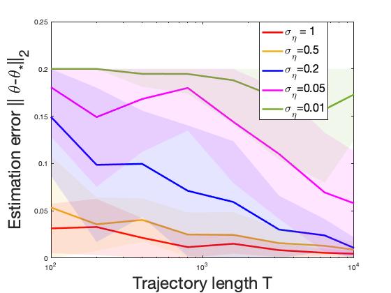
(a) Constrained LQR

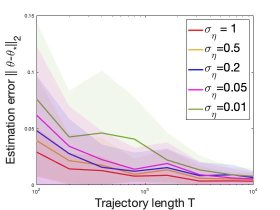
(b) Constrained LQ Tracking

Figure 1: The figures plot the estimation error of $\tilde{\theta}$ when applying $u_{t}=\pi_{\text{RMPC}}(x_{t})+\eta_{t}$ under different excitation levels $\sigma_{\eta}$. Figure (a) considers the constrained LQR in (6), so $\pi_{\text{RMPC}}(x_{t})$ is time-invariant. Figure (b) considers a time-varying tracking problem, so $\pi_{\text{RMPC}}(x_{t})$ is time-varying. The solid lines represent the sample mean. The shades represent one standard deviation.

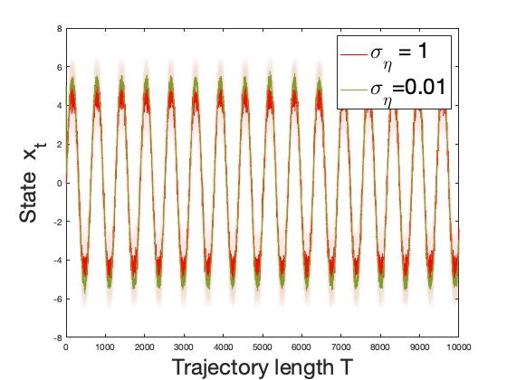
(a) $x_{t}$ trajectories

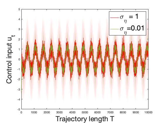
(b) $u_{t}$ trajectories

Figure 2: The solid lines represent the sample means and the shades contain all possible trajectories of states and actions generated by RMPC in the tracking problem.

In this section, we provide numerical experiments to supplement our theoretical analysis by learning with RMPC policies as reviewed in Section 4.

In our experiment, we consider a linear system (2) with $A_{*}=1.2$, $B_{*}=0.9$, and a model uncertainty set $\Theta_{0}=[1,1.2]\times[0.9,1.1]$. The system disturbances $w_{t}$ are i.i.d. following a Uniform distribution on $[-1,1]$. We apply the basic tube-based RMPC policy reviewed in Section 4 and refer the reader to Rawlings and Mayne (2009) for more details. We let the initial estimator in RMPC (7) be $A_{0}=1.1,B_{0}=1$. We generate the excitation noises by $\eta_{t}=\sigma_{\eta}\tilde{\eta}_{t}$, where $\sigma_{\eta}$ represents the excitation level and the variance of $\eta_{t}$, and $\tilde{\eta}_{t}$ are i.i.d. generated from a Uniform distribution on $\{-1,1\}$. We consider the state constraint and the control input constraints as $[-10,10]$. We let the RMPC lookahead window be $W=5$. We repeat each experiment for 15 times.

We consider two types of problems: (a) the constrained LQR problem as reviewed in Section 4 and (b) the constrained LQ tracking problem with a time-varying cost function $(x_{t}-g_{t})^{\top}Q(x_{t}-g_{t})+u_{t}^{\top}Ru_{t}$, where we generate the target trajectory by $g_{t}=8\sin(t/100)$. In the constrained LQR problem, the RMPC policy is time-invariant and nonlinear. In the constrained LQ tracking problem, the RMPC policy is both time-varying and nonlinear.

In Figure 1, we plot the estimation errors of both constrained LQR and constrained LQ tracking under different excitation levels. We observe that, in both cases, the estimation errors decrease with the trajectory lengths $T$. Besides, the estimation errors tend to be smaller if the excitation level $\sigma_{\eta}$ is larger. Both observations above are consistent with Theorem 3.1. It is worth noting that the excitation level $\sigma_{\eta}$ cannot be too large otherwise, the RMPC problem (7) becomes infeasible. Interestingly, in this case, the LQ tracking problem yields a smaller estimation error. This is because the tracking of the moving target helps with the system exploration in this setting.

In Figure 2, we plot the state and control input trajectories in the constrained LQ tracking problem under different levels of excitation noises. Figure 2 demonstrates that RMPC guarantees constraint satisfaction under the model uncertainties and excitation noises even when the target drives the state towards the boundaries of the constraints, thus validating our Assumption 2.1. Further, with a larger excitation level $\sigma_{\eta}$, the possible region of the trajectories is larger due to more uncertainties in the system.

6 Conclusion

This paper studies the linear system identification by a single-trajectory of data generated by general nonlinear and/or time-varying policies with i.i.d. random excitations. We provide a general estimation error bound for any policies with bounded states and actions. Our bound for general policies is consistent with that for linear policies with respect to the trajectory length, system dimensions, and excitation levels. We apply our results to safe learning with robust model predictive control and conduct numerical experiments. There are many future directions to explore, e.g., (i) applying our results to the adaptive learning of robust MPC to determine the tube sizes and conduct regret analysis, (ii) relaxing the bounded disturbances and bounded trajectories assumptions to (sub)Gaussian disturbances and chance constraints of trajectories, (iii) understanding the fundamental lower bound of this problem, (iv) exploring what structures of nonlinear systems can provide similar identification guarantees, (v) designing active exploration with better estimation performance, and (iv) studying the estimation guarantees of other methods, e.g., set membership.

Appendix A Proof of Lemma 3.5

We first consider $w_{t}$. For any fixed $\lambda$ such that $\|\lambda\|_{2}=1$, we define $y=\lambda^{\top}w_{t}$. By Assumption 2.2, we have $\operatorname*{\mathbb{E}}y^{2}=E\lambda^{\top}w_{t}w_{t}^{\top}\lambda=\lambda^{\top}\text{cov}(w_{t})\lambda\geq\sigma_{w}^{2}$ and $|y|\leq\|\lambda\|_{2}\|w_{t}\|_{2}\leq w_{\max}$. Therefore, $\operatorname*{\mathbb{E}}|y|\geq\operatorname*{\mathbb{E}}y^{2}/w_{\max}\geq\sigma_{w}^{2}/w_{\max}.$ By leveraging the inequality above and $\operatorname*{\mathbb{E}}y=0$, we obtain $\operatorname*{\mathbb{E}}y\mathds{1}_{(y\geq 0)}=\frac{1}{2}(\operatorname*{\mathbb{E}}|y|+\operatorname*{\mathbb{E}}y)\geq\frac{\sigma_{w}^{2}}{2w_{\max}}$. Further, we have

$$\frac{\sigma_{w}^{2}}{2w_{\max}} \leq\operatorname*{\mathbb{E}}y\mathds{1}_{(y\geq 0)}$$

$$\leq w_{\max}\mathbb{P}(y\geq\frac{\sigma_{w}^{2}}{4w_{\max}})+\frac{\sigma_{w}^{2}}{4w_{\max}}\mathbb{P}(0\leq y<\frac{\sigma_{w}^{2}}{4w_{\max}})$$

$$\leq w_{\max}\mathbb{P}(y\geq\frac{\sigma_{w}^{2}}{4w_{\max}})+\frac{\sigma_{w}^{2}}{4w_{\max}}$$

By rearranging the terms, we obtain $\mathbb{P}(y\geq s_{w})\geq p_{w}$, where $s_{w}=\frac{\sigma_{w}^{2}}{4w_{\max}}=\frac{\sigma_{w}}{4\bar{w}}$ and $p_{w}=\frac{\sigma_{w}^{2}}{4w_{\max}^{2}}=\frac{1}{4\bar{w}^{2}}$. The proof for $\eta_{t}$ is the same.∎

References

• Bai et al. (1998) Bai, E.W., Cho, H., and Tempo, R. (1998). Convergence properties of the membership set. Automatica, 34(10), 1245–1249.
• Boyd and Sastry (1986) Boyd, S. and Sastry, S.S. (1986). Necessary and sufficient conditions for parameter convergence in adaptive control. Automatica, 22(6), 629–639.
• Dean et al. (2018) Dean, S., Mania, H., Matni, N., Recht, B., and Tu, S. (2018). Regret bounds for robust adaptive control of the linear quadratic regulator. In Advances in Neural Information Processing Systems, 4188–4197.
• Dean et al. (2019a) Dean, S., Mania, H., Matni, N., Recht, B., and Tu, S. (2019a). On the sample complexity of the linear quadratic regulator. Foundations of Computational Mathematics, 1–47.
• Dean et al. (2019b) Dean, S., Tu, S., Matni, N., and Recht, B. (2019b). Safely learning to control the constrained linear quadratic regulator. In 2019 American Control Conference (ACC), 5582–5588. IEEE.
• Dogan et al. (2021) Dogan, I., Shen, Z.J.M., and Aswani, A. (2021). Regret analysis of learning-based mpc with partially-unknown cost function. arXiv preprint arXiv:2108.02307.
• Fisac et al. (2018) Fisac, J.F., Akametalu, A.K., Zeilinger, M.N., Kaynama, S., Gillula, J., and Tomlin, C.J. (2018). A general safety framework for learning-based control in uncertain robotic systems. IEEE Transactions on Automatic Control, 64(7), 2737–2752.
• Fogel and Huang (1982) Fogel, E. and Huang, Y.F. (1982). On the value of information in system identification—bounded noise case. Automatica, 18(2), 229–238.
• Foster et al. (2020) Foster, D., Sarkar, T., and Rakhlin, A. (2020). Learning nonlinear dynamical systems from a single trajectory. In Learning for Dynamics and Control, 851–861. PMLR.
• Köhler et al. (2019) Köhler, J., Andina, E., Soloperto, R., Müller, M.A., and Allgöwer, F. (2019). Linear robust adaptive model predictive control: Computational complexity and conservatism. In 2019 IEEE 58th Conference on Decision and Control (CDC), 1383–1388. IEEE.
• Li et al. (2021a) Li, Y., Das, S., and Li, N. (2021a). Online optimal control with affine constraints. In Proceedings of the AAAI Conference on Artificial Intelligence, volume 35, 8527–8537.
• Li et al. (2021b) Li, Y., Das, S., Shamma, J., and Li, N. (2021b). Safe adaptive learning-based control for constrained linear quadratic regulators with regret guarantees. arXiv preprint arXiv:2111.00411.
• Limón et al. (2010) Limón, D., Alvarado, I., Alamo, T., and Camacho, E.F. (2010). Robust tube-based mpc for tracking of constrained linear systems with additive disturbances. Journal of Process Control, 20(3), 248–260.
• Lopez et al. (2020) Lopez, B.T., Slotine, J.J.E., and How, J.P. (2020). Robust adaptive control barrier functions: An adaptive and data-driven approach to safety. IEEE Control Systems Letters, 5(3), 1031–1036.
• Lorenzen et al. (2019) Lorenzen, M., Cannon, M., and Allgöwer, F. (2019). Robust mpc with recursive model update. Automatica, 103, 461–471.
• Mania et al. (2022) Mania, H., Jordan, M.I., and Recht, B. (2022). Active learning for nonlinear system identification with guarantees. Journal of Machine Learning Research, 23(32), 1–30.
• Mhammedi et al. (2020) Mhammedi, Z., Foster, D.J., Simchowitz, M., Misra, D., Sun, W., Krishnamurthy, A., Rakhlin, A., and Langford, J. (2020). Learning the linear quadratic regulator from nonlinear observations. Advances in Neural Information Processing Systems, 33, 14532–14543.
• Oldewurtel et al. (2008) Oldewurtel, F., Jones, C.N., and Morari, M. (2008). A tractable approximation of chance constrained stochastic mpc based on affine disturbance feedback. In 2008 47th IEEE conference on decision and control, 4731–4736. IEEE.
• Oymak (2019) Oymak, S. (2019). Stochastic gradient descent learns state equations with nonlinear activations. In A. Beygelzimer and D. Hsu (eds.), Proceedings of the Thirty-Second Conference on Learning Theory, volume 99 of Proceedings of Machine Learning Research, 2551–2579. PMLR.
• Oymak and Ozay (2019) Oymak, S. and Ozay, N. (2019). Non-asymptotic identification of lti systems from a single trajectory. In 2019 American control conference (ACC), 5655–5661. IEEE.
• Rawlings and Mayne (2009) Rawlings, J.B. and Mayne, D.Q. (2009). Model predictive control: Theory and design. Nob Hill Pub.
• Salehi et al. (2022) Salehi, I., Taplin, T., and Dani, A. (2022). Learning discrete-time uncertain nonlinear systems with probabilistic safety and stability constraints. IEEE Open Journal of Control Systems.
• Sarkar and Rakhlin (2019) Sarkar, T. and Rakhlin, A. (2019). Near optimal finite time identification of arbitrary linear dynamical systems. In International Conference on Machine Learning, 5610–5618. PMLR.
• Sattar and Oymak (2022) Sattar, Y. and Oymak, S. (2022). Non-asymptotic and accurate learning of nonlinear dynamical systems. Journal of Machine Learning Research, 23(140), 1–49.
• Sattar et al. (2022) Sattar, Y., Oymak, S., and Ozay, N. (2022). Finite sample identification of bilinear dynamical systems. arXiv preprint arXiv:2208.13915.
• Simchowitz et al. (2018) Simchowitz, M., Mania, H., Tu, S., Jordan, M.I., and Recht, B. (2018). Learning without mixing: Towards a sharp analysis of linear system identification. In Conference On Learning Theory, 439–473. PMLR.
• Taylor et al. (2020) Taylor, A.J., Singletary, A., Yue, Y., and Ames, A.D. (2020). A control barrier perspective on episodic learning via projection-to-state safety. IEEE Control Systems Letters, 5(3), 1019–1024.
• Wabersich and Zeilinger (2018) Wabersich, K.P. and Zeilinger, M.N. (2018). Linear model predictive safety certification for learning-based control. In 2018 IEEE Conference on Decision and Control (CDC), 7130–7135. IEEE.
• Wabersich and Zeilinger (2020) Wabersich, K.P. and Zeilinger, M.N. (2020). Performance and safety of bayesian model predictive control: Scalable model-based rl with guarantees. arXiv preprint arXiv:2006.03483.
• Xu (2018) Xu, X. (2018). Constrained control of input–output linearizable systems using control sharing barrier functions. Automatica, 87, 195–201.
• Zhao and Li (2022) Zhao, Z. and Li, Q. (2022). Adaptive sampling methods for learning dynamical systems. In Mathematical and Scientific Machine Learning, 335–350. PMLR.
• Ziemann and Tu (2022) Ziemann, I. and Tu, S. (2022). Learning with little mixing. arXiv preprint arXiv:2206.08269.