DCdetector: Dual Attention Contrastive Representation Learning
for Time Series Anomaly Detection

Abstract.

Time series anomaly detection is critical for a wide range of applications. It aims to identify deviant samples from the normal sample distribution in time series. The most fundamental challenge for this task is to learn a representation map that enables effective discrimination of anomalies. Reconstruction-based methods still dominate, but the representation learning with anomalies might hurt the performance with its large abnormal loss. On the other hand, contrastive learning aims to find a representation that can clearly distinguish any instance from the others, which can bring a more natural and promising representation for time series anomaly detection. In this paper, we propose DCdetector, a multi-scale dual attention contrastive representation learning model. DCdetector utilizes a novel dual attention asymmetric design to create the permutated environment and pure contrastive loss to guide the learning process, thus learning a permutation invariant representation with superior discrimination abilities. Extensive experiments show that DCdetector achieves state-of-the-art results on multiple time series anomaly detection benchmark datasets. Code is publicly available at this URL.

1. Introduction

Time series anomaly detection is widely used in real-world applications, including but not limited to industrial equipment status monitoring, financial fraud detection, fault diagnosis, and daily monitoring and maintenance of automobiles (Cook et al., 2019; Ren et al., 2019; Anandakrishnan et al., 2018; Golmohammadi and Zaiane, 2015; Yang et al., 2021b). With the rapid development of different sensors, large-scale time series data has been collected during the system’s running time in many different applications (Wen et al., 2022; Li et al., 2021a; Yang et al., 2023). Effectively discovering abnormal patterns in systems is crucial to ensure security and avoid economic losses (Yang et al., 2021d). For example, in the energy industry, detecting anomalies in wind turbine sensors in time helps to avoid catastrophic failure. In the financial industry, detecting fraud is essential for reducing pecuniary loss.

However, it is challenging to discover abnormal patterns from a mass of complex time series. Firstly, it is still being determined what the anomalies will be like. Anomaly is also called outlier or novelty, which means observation unusual, irregular, inconsistent, unexpected, rare, faulty, or simply strange depending on the situation (Ruff et al., 2021). Moreover, the typical situation is usually complex, which makes it harder to define what is unusual or unexpected. For instance, the wind turbine works in different patterns with different weather situations. Secondly, anomalies are usually rare, so it takes work to get labels (Yang et al., 2021c). Most supervised or semi-supervised methods fail to work given limited labeled training data. Third, anomaly detection models should consider temporal, multidimensional, and non-stationary features for time series data (Yang et al., 2021a). Multidimensionality describes that there is usually a dependence among dimensions in multivariate time series, and non-stationarity means the statistical features of time series are unstable. Specifically, temporal dependency means the adjacent points have latent dependence on each other. Although every point should be labeled as normal or abnormal, it is not reasonable to consider a single point as a sample.

Researchers have designed various time-series anomaly detection methods to deal with these challenges. They can be roughly classified as statistical, classic machine learning, and deep learning-based methods (Blázquez-García et al., 2021; Ruff et al., 2021). Machine learning methods, especially deep learning-based methods, have succeeded greatly due to their powerful representation advantages. Most of the supervised and semi-supervised methods (Zhang et al., 2022c; Chauhan and Vig, 2015; Chen et al., 2021a; Park et al., 2018; Niu et al., 2020; Zhao et al., 2020b) can not handle the challenge of limited labeled data, especially the anomalies are dynamic and new anomalies never observed before may occur. Unsupervised methods are popular without strict requirements on labeled data, including one class classification-based, probabilistic-based, distance-based, forecasting-based, reconstruction-based approaches (Deng and Hooi, 2021b; Zong et al., 2018; Su et al., 2019; Li et al., 2022; Campos et al., 2021; Zamanzadeh Darban et al., 2022; Ruff et al., 2021).

Reconstruction-based methods learn a model to reconstruct normal samples, and thereby the instances failing be reconstructed by the learned model are anomalies. Such an approach is developing rapidly due to its power in handling complex data by combining it with different machine learning models and its interpretability that the instances behave unusually abnormally. However, it is usually challenging to learn a well-reconstructed model for normal data without being obstructed by anomalies. The situation is even worse in time series anomaly detection as the number of anomalies is unknown, and normal and abnormal points may appear in one instance, making it harder to learn a clean, well-reconstructed model for normal points.

Recently, contrastive representative learning has attracted attention due to its diverse design and outstanding performance in downstream tasks in the computer vision field (Ye et al., 2019; He et al., 2020; Chen et al., 2020; Caron et al., 2020). However, the effectiveness of contrastive representative learning still needs to be explored in the time-series anomaly detection area. In this paper, we propose a Dual attention Contrastive representation learning anomaly detector called DCdetector to handle the challenges in time series anomaly detection. The key idea of our DCdetector is that normal time series points share the latent pattern, which means normal points have strong correlations with other points. In contrast, the anomalies do not (i.e., weak correlations with others). Learning consistent representations for anomalies from different views will be hard but easy for normal points. The primary motivation is that if normal and abnormal points’ representations are distinguishable, we can detect anomalies without a highly qualified reconstruction model.

Specifically, we propose a contrastive structure with two branches and a dual attention module, and two branches share network weights. This model is trained based on the similarity of two branches, as normal points are the majority. The representation inconsistency of anomaly will be conspicuous. Thus, the representation difference between normal and abnormal data is enlarged without a highly qualified reconstruction model. To capture the temporal dependency in time series, DCdetector utilizes patching-based attention networks as the basic module. A multi-scale design is proposed to reduce information loss during patching. DCdetector takes all channels into representation efficiently with a channel independence design for multivariate time series. In particular, DCdetector does not require prior knowledge about anomalies and thus can handle new outliers never observed before. The main contributions of our DCdetector are summarized as follows:

• Architecture: A contrastive learning-based dual-branch attention structure is designed to learn a permutation invariant representation that enlarges the representation differences between normal points and anomalies. Also, channel independence patching is proposed to enhance local semantic information in time series. Multi-scale is proposed in the attention module to reduce information loss during patching.

• Optimization: An effective and robust loss function is designed based on the similarity of two branches. Note that the model is trained purely contrastively without reconstruction loss, which reduces distractions from anomalies.

• Performance & Justification: DCdetector achieves performance comparable or superior to state-of-the-art methods on seven multivariate and one univariate time series anomaly detection benchmark datasets. We also provide justification discussion to explain how our model avoids collapse without negative samples.

2. Related Work

In this section, we show the related literature for this work. The relevant works include anomaly detection and contrastive representation learning.

Time Series Anomaly Detection

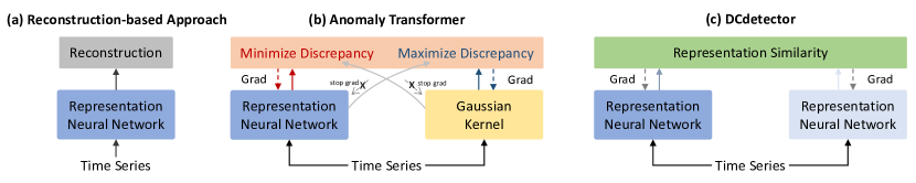
Figure 1. Architecture comparison of three approaches. The reconstruction-based approach uses a representation neural network to learn the pattern of normal points and do reconstruction. In Anomaly Transformer, the prior discrepancy is learned with Gaussian Kernel and the association discrepancy is learned with a transformer module; MinMax association learning is also critical and reconstruction loss is contained. DCdetector is concise without a specially designed Gaussian Kernel or a MinMax learning strategy, nor a reconstruction loss.

There are various approaches to detect anomalies in time series, including statistical methods, classical machine learning methods, and deep learning methods (Schmidl et al., 2022). Statistical methods include using moving averages, exponential smoothing (Phillips and Jin, 2015), and the autoregressive integrated moving average (ARIMA) model (Box and Pierce, 1970). Machine learning methods include clustering algorithms such as k-means (Kant and Mahajan, 2019) and density-based methods, as well as classification algorithms such as decision trees (Liu et al., 2008; Karczmarek et al., 2020) and support vector machines (SVMs). Deep learning methods include using autoencoders, variational autoencoders (VAEs) (Sakurada and Yairi, 2014; Park et al., 2018), and recurrent neural networks (RNNs) (Canizo et al., 2019; Su et al., 2019) such as long short-term memory (LSTM) networks (Zamanzadeh Darban et al., 2022). Recent works in time series anomaly detection also include generative adversarial networks (GANs) based methods (Li et al., 2019a; Zhou et al., 2019; Chen et al., 2021b, b) and deep reinforcement learning (DRL) based methods (Yu and Sun, 2020; Huang et al., 2018). In general, deep learning methods are more effective in identifying anomalies in time series data, especially when the data is high-dimensional or non-linear.

In another view, time series anomaly detection models can be roughly divided into two categories: supervised and unsupervised anomaly detection algorithms. Supervised methods can perform better when the anomaly label is available or affordable. Such methods can be dated back to AutoEncoder (Sakurada and Yairi, 2014), LSTM-VAE (Park et al., 2018), Spectral Residual (SR) (Ren et al., 2019), RobustTAD (Gao et al., 2020) and so on. On the other hand, an unsupervised anomaly detection algorithm can be applied in cases where the anomaly labels are difficult to obtain. Such versatility results in the community’s long-lasting interest in developing new unsupervised time-series anomaly detection methods, including DAGMM (Zong et al., 2018), OmniAnomaly (Su et al., 2019), GDN (Deng and Hooi, 2021b), RDSSM (Li et al., 2022) and so on. Unsupervised deep learning methods have been widely studied in time series anomaly detection. The main reasons are as follows. First, it is usually hard or unaffordable to get labels for all time series sequences in real-world applications. Second, deep models are powerful in representation learning and have the potential to get a decent detection accuracy under the unsupervised setting. Most of them are based on a reconstruction approach where a well-reconstructed model is learned for normal points; Then, the instances failing to be reconstructed are anomalies. Recently, some self-supervised learning-based methods have been proposed to enhance the generalization ability in unsupervised anomaly detection (Zhao et al., 2020b; Jiao et al., 2022; Zhang et al., 2022a).

Contrastive Representation Learning

The goal of contrastive representation learning is to learn an embedding space in which similar data samples stay close to each other while dissimilar ones are far apart. The idea of contrastive learning can be traced back to InstDic (Wu et al., 2018). Classical contrastive models create ¡positive, negative¿ sample pairs to learn a representation where positive samples are near each other (pulled together) and far from negative samples (pushed apart) (Ye et al., 2019; He et al., 2020; Chen et al., 2020; Caron et al., 2020). Their key designs are about how to define negative samples and deal with the high computation power/large batches requirements (Khan et al., 2022). On the other hand, BYOL (Grill et al., 2020) and SimSiam (Chen and He, 2021) get rid of negative samples involved, and such a simple siamese model (SimSiam) achieves comparable performance with other state-of-the-art complex architecture.

It is illuminating to make the distance of two-type samples larger using contrastive design. We try to distinguish time series anomalies and normal points with a well-designed multi-scale patching-based attention module. Moreover, our DCdetector is also free from negative samples and does not fall into a trivial solution even without the ”stop gradient”.

3. Methodology

Consider a multivariate time-series sequence of length T:

$${\mathcal{X}=(x_{1},x_{2},\ldots,x_{T}),}$$

where each data point $x_{t}\in{\rm I\!R}^{d}$ is acquired at a certain timestamp $t$ from industrial sensors or machines, and $d$ is the data dimensionality, e.g., the number of sensors or machines. Our problem can be regarded as given input time-series sequence $\mathcal{X}$, for another unknown test sequence $\mathcal{X}_{test}$ of length $T^{\prime}$ with the same modality as the training sequence, we want to predict $\mathcal{Y}_{test}=(y_{1},y_{2},\ldots,y_{T^{\prime}})$. Here $y_{t}\in\{0,1\}$ where 1 denotes an anomalous data point and 0 denotes a normal data point.

As mentioned previously, representation learning is a powerful tool to handle the complex pattern of time series. Due to the high cost of gaining labels in practice, unsupervised and self-supervised methods are more popular. The critical issue in time series anomaly detection is to distinguish anomalies from normal points. Learning representations that demonstrate wide disparities without anomalies is promising. We amplify the advantages of contrastive representation learning with a dual attention structure.

In some way, the underlining inductive bias we used here is similar to what Anomaly Transformer explored (Xu et al., 2021). That is, anomalies have less connection or interaction with the whole series than their adjacent points. The Anomaly Transformer detects anomalies by association discrepancy between a learned Gaussian kernel and attention weight distribution. In contrast, we proposed DCdetector, which achieves a similar goal in a much more general and concise way with a dual-attention self-supervised contrastive-type structure.

To better position our work in the landscape of time series anomaly detection, we give a brief comparison of three approaches. To be noticed, Anomaly Transformer is a representation of a series of explicit association modeling works (Cheng et al., 2009; Zhao et al., 2020a; Deng and Hooi, 2021a; Boniol and Palpanas, 2020), not implying it is the only one. We merely want to make a more direct comparison with the closest work here. Figure 1 shows the architecture comparison of three approaches. The reconstruction-based approach (Figure 1(a)) uses a representation neural network to learn the pattern of normal points and do reconstruction. Anomaly Transformer (Figure 1(b)) takes advantage of the observation that it is difficult to build nontrivial associations from abnormal points to the whole series. Thereby, the prior discrepancy is learned with Gaussian Kernel and the association discrepancy is learned with a transformer module. MinMax association learning is also critical for Anomaly Transformer and reconstruction loss is contained. In contrast, the proposed DCdetector (Figure 1(c)) is concise, in the sense that it does not need a specially designed Gaussian Kernel, a MinMax learning strategy, or a reconstruction loss. The DCdetector mainly leverages the designed contrastive learning-based dual-branch attention for discrepancy learning of anomalies in different views to enlarge the differences between anomalies and normal points. The simplicity and effectiveness contribute to DCdetector’s versatility.

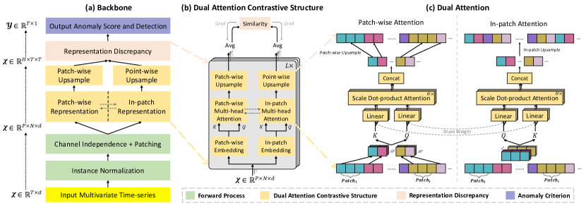
Figure 2. The workflow of the DCdetector framework. DCdetector consists of four main components: Forward Process module, Dual Attention Contrastive Structure module, Representation Discrepancy module, and Anomaly Criterion module.

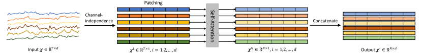
Figure 3. Basic patching attention with channel independence. Each channel in the multivariate time series input is considered as a single time series and divided into patches. Each channel shares the same self-attention network, and the representation results are concatenated as the final output.

3.1. Overall Architecture

Figure 2 shows the overall architecture of the DCdetector, which consists of four main components, Forward Process module, Dual Attention Contrastive Structure module, Representation Discrepancy module, and Anomaly Criterion module.

The input multivariate time series in the Forward Process module is normalized by an instance normalization (Kim et al., 2021; Ulyanov et al., 2017) module. The inputs to the instance normalization all come from the independent channels themselves. It can be seen as a consolidation and adjustment of global information, and a more stable approach to training processing. Channel independence assumption has been proven helpful in multivariate time series forecasting tasks (Salinas et al., 2020; Li et al., 2019b) to reduce parameter numbers and overfitting issues. Our DCdetector follows such channel independence setting to simplify the attention network with patching.

More specifically, the basic patching attention with channel independence is shown in Figure 3. Each channel in the multivariate time series input ($\mathcal{X}\in{\rm I\!R}^{T\times d}$) is considered as a single time series ($\mathcal{X}^{i}\in{\rm I\!R}^{T\times 1},i=1,2,\dots,d$) and divided into patches. Each channel shares the same self-attention network, and the representation results ($\mathcal{X}^{\prime i}\in{\rm I\!R}^{N\times 1},i=1,2,\dots,d$) is concatenated as the final output ($\mathcal{X}^{\prime}\in{\rm I\!R}^{N\times d}$). In the implementation phase, running a sliding window in time series data is widely used in time series anomaly detection tasks (Shen et al., 2020; Xu et al., 2021) and has little influence on the main design. More implementation details are left in the experiment section.

The Dual Attention Contrastive Structure module is critical in our design. It learns the representation of inputs in different views. The insight is that, for normal points, most of them will share the same latent pattern even in different views (a strong correlation is not easy to be destroyed). However, as anomalies are rare and do not have explicit patterns, it is hard for them to share latent modes with normal points or among themselves (i.e., anomalies have a weak correlation with other points). Thus, the difference will be slight for normal point representations in different views and large for anomalies. We can distinguish anomalies from normal points with a well-designed Representation Discrepancy criterion. The details of Dual Attention Contrastive Structure and Representation Discrepancy are left in the following Section 3.2 and Section 3.3.

As for the Anomaly Criterion, we calculate anomaly scores based on the discrepancy between the two representations and use a prior threshold for anomaly detection. The details are left in Section 3.4.

3.2. Dual Attention Contrastive Structure

In DCdetector, we propose a contrastive representation learning structure with dual attention to get the representations of input time series from different views. Concretely, with the patching operation, DCdetector takes patch-wise and in-patch representations as two views. Note that it differs from traditional contrastive learning, where original and augmented data are considered as two views of the original data. Moreover, DCdetector does not construct ¡positive, negative¿ pairs like the typical contrastive methods (Wu et al., 2018; He et al., 2020). Instead, its basic setting is similar to the contrastive methods only using positive samples (Chen and He, 2021; Grill et al., 2020).

3.2.1. Dual Attention

As shown in Figure 2, input time series $\mathcal{X}\in{\rm I\!R}^{T\times d}$ are patched as $\mathcal{X}\in{\rm I\!R}^{P\times N\times d}$ where $P$ is the size of patches and $N$ is the number of patches. Then, we fuse the channel information with the batch dimension and the input size becomes $\mathcal{X}\in{\rm I\!R}^{P\times N}$. With such patched time series, DCdetector learns representation in patch-wise and in-patch views with self-attention networks. Our dual attention can be encoded in $L$ layers, so for simplicity, we only use one of these layers as an example.

For the patch-wise representation, a single patch is considered as a unit, and the dependencies among patches are modeled by a multi-head self-attention network (named patch-wise attention). In detail, an embedded operation will be applied in the patch_size ($P$) dimension, and the shape of embedding is $\mathcal{X_{N}}\in{\rm I\!R}^{N\times d_{model}}$. Then, we adopt multi-head attention weights to calculate the patch-wise representation. Firstly, initialize the query and key:

(1) $$\mathcal{Q_{N}}_{i},\mathcal{K_{N}}_{i}=\mathcal{W_{Q}}_{i}\mathcal{X_{N}}_{i},\mathcal{W_{K}}_{i}\mathcal{X_{N}}_{i}\quad 1\leq i\leq H,$$

where $\mathcal{Q_{N}}_{i},\mathcal{K_{N}}_{i}\in{\rm I\!R}^{N\times\frac{d_{model}}{H}}$ denote the query and key, respectively, $\mathcal{W_{Q}}_{i},\mathcal{W_{K}}_{i}\in{\rm I\!R}^{\frac{d_{model}}{H}\times\frac{d_{model}}{H}}$ represent learnable parameter matrices of $\mathcal{Q_{N}}_{i},\mathcal{K_{N}}_{i}$, and $H$ is the head number. Then, compute the attention weights:

(2) $$Attn_{\mathcal{N}_{i}}=Softmax(\frac{\mathcal{Q_{N}}_{i}\mathcal{K_{N}}_{i}^{T}}{\sqrt{\frac{d_{model}}{H}}}),$$

where $Softmax(\cdot)$ function normalizes the attention weight. Finally, contact the multi-head and get the final patch-wise representation $Attn_{\mathcal{N}}$, which is:

(3) $$Attn_{\mathcal{N}}=\text{Concat}(Attn_{\mathcal{N}_{1}},\cdots,Attn_{\mathcal{N}_{H}})W_{\mathcal{N}}^{O},$$

where $W_{\mathcal{N}}^{O}\in{\rm I\!R}^{d_{model}\times d_{model}}$ is a learnable parameter matrix.

Similarly, for the in-patch representation, the dependencies of points in the same patch are gained by a multi-head self-attention network (called in-patch attention). Note that the patch-wise attention network shares weights with the in-patch attention network. Specifically, another embedded operation will be applied in the patch_number ($N$) dimension, and the shape of embedding is $\mathcal{X_{P}}\in{\rm I\!R}^{P\times d_{model}}$. Then, we adopt multi-head attention weights to calculate the in-patch representation. First, initialize the query and key:

(4) $$\mathcal{Q_{P}}_{i},\mathcal{K_{P}}_{i}=\mathcal{W_{Q}}_{i}\mathcal{X_{P}}_{i},\mathcal{W_{K}}_{i}\mathcal{X_{P}}_{i}\quad 1\leq i\leq H,$$

where $\mathcal{Q_{P}}_{i},\mathcal{K_{P}}_{i}\in{\rm I\!R}^{P\times\frac{d_{model}}{H}}$ denote the query and key, respectively, and $\mathcal{W_{Q}}_{i},\mathcal{W_{K}}_{i}\in{\rm I\!R}^{\frac{d_{model}}{H}\times\frac{d_{model}}{H}}$ represent learnable parameter matrices of $\mathcal{Q_{P}}_{i},\mathcal{K_{N}}_{i}$. Then, compute the attention weights:

(5) $$Attn_{\mathcal{P}_{i}}=Softmax(\frac{\mathcal{Q_{P}}_{i}\mathcal{K_{P}}_{i}^{T}}{\sqrt{\frac{d_{model}}{H}}}),$$

where $Softmax(\cdot)$ function normalizes the attention weight. Finally, contact the multi-head and get the final in-patch representation $Attn_{\mathcal{P}}$, which is:

(6) $$Attn_{\mathcal{P}}=\text{Concat}(Attn_{\mathcal{P}_{1}},\cdots,Attn_{\mathcal{P}_{H}})W_{\mathcal{P}}^{O},$$

where $W_{\mathcal{P}}^{O}\in{\rm I\!R}^{d_{model}\times d_{model}}$ is a learnable parameter matrix.

Note that the $\mathcal{W_{Q}}_{i},\mathcal{W_{K}}_{i}$ are the shared weights within the in-patch attention representation network and patch-wise attention representation network.

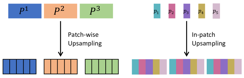
Figure 4. A simple example of how up-sampling is done. For patch-wise branch, repeating is done in patches (from patch to points). For in-patch branch, repeating is done from ”one” patch to a full number of patches (from points to patches).

3.2.2. Up-sampling and Multi-scale Design

Although the patching design benefits from gaining local semantic information, patch-wise attention ignores the relevance among points in a patch, and in-patch attention ignores the relevance among patches. To compare the results of two representation networks, we need to do up-sampling first. For the patch-wise branch, as we only have the dependencies among patches, repeating is done inside patches (i.e., from patch to points) for up-sampling, and we will get the final patch-wise representation $\mathcal{N}$. For the in-patch branch, as only dependencies among patch points are gained, repeating is done from ”one” patch to a full number of patches, and we will get the final in-patch representation $\mathcal{P}$.

A simple example is shown in Figure 4 where a patch is noted as $P^{i}$, and a point is noted as $p_{i}$. Such patching and repeating up-sampling operations inevitably lead to information loss. To keep the information from the original data better, DCdetector introduces a multi-scale design for patching representation and up-sampling. The final representation concatenates results in different scales (i.e., patch sizes). Specifically, we can preset a list of various patches to perform parallel patching and the computation of dual attention representations, simultaneously. After upsampling each patch part, they are summed to obtain the final patch-wise representation $\mathcal{N}$ and in-patch representation $\mathcal{P}$, which are

(7) $$\mathcal{N}=\text{Upsampling}(Attn_{\mathcal{N}}),\quad\mathcal{P}=\text{Upsampling}(Attn_{\mathcal{P}}).$$

3.2.3. Contrastive Structure

Patch-wise and in-patch branches output representations of the same input time series in two different views. As shown in Figure 2 (c), patch-wise sample representation learns a weighted combination between sample points in the same position from each patch. In-patch sample representation, on the other hand, learns a weighted combination between points within the same patch. We can treat these two representations as permutated multi-view representations. The key inductive bias we exploit here is that normal points can maintain their representation under permutations while the anomalies can not. From such dual attention non-negative contrastive learning, we want to learn a permutation invariant representation. Learning details are left in Section 3.3.

3.3. Representation Discrepancy

With dual attention contrastive structure, representations from two views (patch-wise branch and in-patch branch) are gained. We formalize a loss function based on Kullback–Leibler divergence (KL divergence) to measure the similarity of such two representations. The intuition is that, as anomalies are rare and normal points share latent patterns, the same inputs’ representations should be similar.

3.3.1. Loss function definition

The loss function of the $\mathcal{P}$ and $\mathcal{N}$ can then be defined as

(8) $$\mathcal{L_{P}}\{\mathcal{P},\mathcal{N};\mathcal{X}\}=\sum KL(\mathcal{P},\text{Stopgrad}(\mathcal{N}))+KL(\text{Stopgrad}(\mathcal{N}),\mathcal{P}),$$

(9) $$\mathcal{L_{N}}\{\mathcal{P},\mathcal{N};\mathcal{X}\}=\sum KL(\mathcal{N},\text{Stopgrad}(\mathcal{P}))+KL(\text{Stopgrad}(\mathcal{P}),\mathcal{N}),$$

where $\mathcal{X}$ is the input time series, $KL(\cdot||\cdot)$ is the KL divergence distance, $\mathcal{P}$ and $\mathcal{N}$ are the representation result matrices of the in-patch branch and the patch-wise branch, respectively. Stop-gradient (labeled as ’Stopgrad’) operation is also used in our loss function to train two branches asynchronously. Then, the total loss function $\mathcal{L}$ is defined as

(10) $$\mathcal{L}=\frac{\mathcal{L_{N}}-\mathcal{L_{P}}}{len(\mathcal{N})}.$$

Unlike most anomaly detection works based on reconstruction framework (Ruff et al., 2021), DCdetector is a self-supervised framework based on representation learning, and no reconstruction part is utilized in our model. There is no doubt that reconstruction helps to detect the anomalies which behave not as expected. However, it is not easy to build a suitable encoder and decoder to ’reconstruct’ the time series as they are expected to be with anomalies’ interference. Moreover, the ability of representation is restricted as the latent pattern information is not fully considered.

3.3.2. Discussion about Model Collapse

Interestingly, with only single-type inputs (or saying, no negative samples included), our DCdetector model does not fall into a trivial solution (model collapse). SimSiam (Chen and He, 2021) gives the main credit for avoiding model collapse to stop gradient operation in their setting. However, we find that DCdetector still works without stop gradient operation, although with the same parameters, the no stop gradient version does not gain the best performance. Details are shown in the ablation study (Section 4.5.1).

A possible explanation is that our two branches are totally asymmetric. Following the unified perspective proposed in (Zhang et al., 2022b), consider the output vector of a branch as $Z$ and $Z$ can be decomposed into two parts $o$ and $r$ as $Z=o+r$, where $o={\rm I\!E}[Z]$ is the center vector defined as an average of $Z$ in the whole representation space, and $r$ is the residual vector. When the collapse happens, all vectors $Z$ fall into the center vector $o$ and $o$ dominates over $r$. With two branches noted as $Z_{p}=o_{p}+r_{p}$, $Z_{n}=o_{n}+r_{n}$, if the branches are symmetric, i.e., $o_{p}=o_{n}$, then the distance between them is $Z_{p}-Z_{n}=r_{p}-r_{n}$. As $r_{p}$ and $r_{n}$ come from the same input example, it will lead to collapse. Fortunately, the two branches in DCdetector are asymmetric, so it is not easy for $o_{p}$ to be the same as $o_{n}$ even when $r_{p}$ and $r_{n}$ are similar. Thus, due to our asymmetric design, DCdetector is hard to fall into a trivial solution.

3.4. Anomaly Criterion

With the insight that normal points usually share latent patterns (with strong correlation among them), thus the distances of representation results from different views for normal points are less than that for anomalies. The final anomaly score of $\mathcal{X}\in{\rm I\!R}^{T\times d}$ is defined as

(11) $$\text{AnomalyScore}(\mathcal{X})=\sum KL(\mathcal{P},\text{Stopgrad}(\mathcal{N}))+KL(\mathcal{N},\text{Stopgrad}(\mathcal{P})).$$

It is a point-wise anomaly score, and anomalies result in higher scores than normal points.

Based on the point-wise anomaly score, a hyperparameter threshold $\delta$ is used to decide if a point is an anomaly (1) or not (0). If the score exceeds the threshold, the output $\mathcal{Y}$ is an anomaly. That is

(12) $$\mathcal{Y}_{i}=\begin{cases}\text{1: anomaly}\quad\text{AnomalyScore}(\mathcal{X}_{i})\geq\delta\\ \text{0: normal}\quad\quad\!\!\!\text{AnomalyScore}(\mathcal{X}_{i})<\delta.\end{cases}$$

4. Experiments

4.1. Benchmark Datasets

We adopt eight representative benchmarks from five real-world applications to evaluate DCdetector: (1) MSL (Mars Science Laboratory dataset) is collected by NASA and shows the condition of the sensors and actuator data from the Mars rover (Hundman et al., 2018). (2) SMAP (Soil Moisture Active Passive dataset) is also collected by NASA and presents the soil samples and telemetry information used by the Mars rover (Hundman et al., 2018). Compared with MSL, SMAP has more point anomalies. (3) PSM (Pooled Server Metrics dataset) is a public dataset from eBay Server Machines with 25 dimensions (Abdulaal et al., 2021). (4) SMD (Server Machine Dataset) is a five-week-long dataset collected from an internet company compute cluster, which stacks accessed traces of resource utilization of 28 machines (Su et al., 2019). (5) SWaT (Secure Water Treatment) is a 51-dimension sensor-based dataset collected from critical infrastructure systems under continuous operations (Mathur and Tippenhauer, 2016). (6) NIPS-TS-SWAN is an openly accessible comprehensive, multivariate time series benchmark extracted from solar photospheric vector magnetograms in Spaceweather HMI Active Region Patch series (Angryk et al., 2020; Lai et al., 2021). (7) NIPS-TS-GECCO is a drinking water quality dataset for the ‘internet of things’, which is published in the 2018 genetic and evolutionary computation conference (Moritz et al., 2018; Lai et al., 2021). Besides the above multivariate time series datasets, we also test univariate time series datasets. (8) UCR is provided by the Multi-dataset Time Series Anomaly Detection Competition of KDD2021, and contains 250 sub-datasets from various natural sources (Dau et al., 2019; Keogh et al., 2021). It is a univariate time series of dataset subsequence anomalies. In each time series, there is one and only one anomaly. More details of the eight benchmark datasets are summarized in Table 8 in Appendix B.

Table 1. Overall results on real-world multivariate datasets. Performance ranked from lowest to highest. The P, R and F1 are the precision, recall and F1-score. All results are in %, the best ones are in Bold, and the second ones are underlined.

Dataset	SMD			MSL			SMAP			SWaT			PSM
Metric	P	R	F1	P	R	F1	P	R	F1	P	R	F1	P	R	F1
LOF	56.34	39.86	46.68	47.72	85.25	61.18	58.93	56.33	57.60	72.15	65.43	68.62	57.89	90.49	70.61
OCSVM	44.34	76.72	56.19	59.78	86.87	70.82	53.85	59.07	56.34	45.39	49.22	47.23	62.75	80.89	70.67
U-Time	65.95	74.75	70.07	57.20	71.66	63.62	49.71	56.18	52.75	46.20	87.94	60.58	82.85	79.34	81.06
IForest	42.31	73.29	53.64	53.94	86.54	66.45	52.39	59.07	55.53	49.29	44.95	47.02	76.09	92.45	83.48
DAGMM	67.30	49.89	57.30	89.60	63.93	74.62	86.45	56.73	68.51	89.92	57.84	70.40	93.49	70.03	80.08
ITAD	86.22	73.71	79.48	69.44	84.09	76.07	82.42	66.89	73.85	63.13	52.08	57.08	72.80	64.02	68.13
VAR	78.35	70.26	74.08	74.68	81.42	77.90	81.38	53.88	64.83	81.59	60.29	69.34	90.71	83.82	87.13
MMPCACD	71.20	79.28	75.02	81.42	61.31	69.95	88.61	75.84	81.73	82.52	68.29	74.73	76.26	78.35	77.29
CL-MPPCA	82.36	76.07	79.09	73.71	88.54	80.44	86.13	63.16	72.88	76.78	81.50	79.07	56.02	99.93	71.80
TS-CP2	87.42	66.25	75.38	86.45	68.48	76.42	87.65	83.18	85.36	81.23	74.10	77.50	82.67	78.16	80.35
Deep-SVDD	78.54	79.67	79.10	91.92	76.63	83.58	89.93	56.02	69.04	80.42	84.45	82.39	95.41	86.49	90.73
BOCPD	70.9	82.04	76.07	80.32	87.20	83.62	84.65	85.85	85.24	89.46	70.75	79.01	80.22	75.33	77.70
LSTM-VAE	75.76	90.08	82.30	85.49	79.94	82.62	92.20	67.75	78.10	76.00	89.50	82.20	73.62	89.92	80.96
BeatGAN	72.90	84.09	78.10	89.75	85.42	87.53	92.38	55.85	69.61	64.01	87.46	73.92	90.30	93.84	92.04
LSTM	78.55	85.28	81.78	85.45	82.50	83.95	89.41	78.13	83.39	86.15	83.27	84.69	76.93	89.64	82.80
OmniAnomaly	83.68	86.82	85.22	89.02	86.37	87.67	92.49	81.99	86.92	81.42	84.30	82.83	88.39	74.46	80.83
InterFusion	87.02	85.43	86.22	81.28	92.70	86.62	89.77	88.52	89.14	80.59	85.58	83.01	83.61	83.45	83.52
THOC	79.76	90.95	84.99	88.45	90.97	89.69	92.06	89.34	90.68	83.94	86.36	85.13	88.14	90.99	89.54
AnomalyTrans	88.47	92.28	90.33	91.92	96.03	93.93	93.59	99.41	96.41	89.10	99.28	94.22	96.94	97.81	97.37
DCdetector	83.59	91.10	87.18	93.69	99.69	96.60	95.63	98.92	97.02	93.11	99.77	96.33	97.14	98.74	97.94

Table 2. Multi-metrics results on real-world multivariate datasets. Aff-P and Aff-R are the precision and recall of affiliation metric (Huet et al., 2022), respectively. R_A_R and R_A_P are Range-AUC-ROC and Range-AUC-PR (Paparrizos et al., 2022), which denote two scores based on label transformation under ROC curve and PR curve, respectively. V_ROC and V_RR are volumes under the surfaces created based on ROC curve and PR curve (Paparrizos et al., 2022), respectively. All results are in %, and the best ones are in Bold.

Dataset	Method	Acc	F1	Aff-P (Huet et al., 2022)	Aff-R (Huet et al., 2022)	R_A_R (Paparrizos et al., 2022)	R_A_P (Paparrizos et al., 2022)	V_ROC (Paparrizos et al., 2022)	V_PR (Paparrizos et al., 2022)
MSL	AnomalyTrans	98.69	93.93	51.76	95.98	90.04	87.87	88.20	86.26
	DCdetector	99.06	96.60	51.84	97.39	93.17	91.64	93.15	91.66
SMAP	AnomalyTrans	99.05	96.41	51.39	98.68	96.32	94.07	95.52	93.37
	DCdetector	99.21	97.02	51.46	98.64	96.03	94.18	95.19	93.46
SWaT	AnomalyTrans	98.51	94.22	53.03	98.08	97.89	93.47	97.92	93.49
	DCdetector	99.09	96.33	52.40	97.67	96.63	94.06	96.95	94.34
PSM	AnomalyTrans	98.68	97.37	55.35	80.28	91.83	93.03	88.71	90.71
	DCdetector	98.95	97.94	54.71	82.93	91.55	92.93	88.41	90.58

Table 3. Overall results on NIPS-TS datasets. Performance ranked from lowest to highest. All results are in %, the best ones are in bold, and the second ones are underlined.

Dataset	NIPS-TS-GECCO			NIPS-TS-SWAN
Metric	P	R	F1	P	R	F1
OCSVM*	2.1	34.1	4.0	19.3	0.1	0.1
MatrixProfile	4.6	18.5	7.4	16.7	17.5	17.1
GBRT	17.5	14.0	15.6	44.7	37.5	40.8
LSTM-RNN	34.3	27.5	30.5	52.7	22.1	31.2
Autoregression	39.2	31.4	34.9	42.1	35.4	38.5
OCSVM	18.5	74.3	29.6	47.4	49.8	48.5
IForest*	39.2	31.5	39.0	40.6	42.5	41.6
AutoEncoder	42.4	34.0	37.7	49.7	52.2	50.9
AnomalyTrans	25.7	28.5	27.0	90.7	47.4	62.3
IForest	43.9	35.3	39.1	56.9	59.8	58.3
DCdetector	38.3	59.7	46.6	95.5	59.6	73.4

Table 4. Overall results on univariate dataset. Results are in %, and the best ones are in Bold.

Dataset	UCR
Metric	Acc	P	R	F1	Count
AnomalyTrans	99.49	60.41	100	73.08	42
DCdetector	99.51	61.62	100	74.05	46

Table 5. Multi-metrics results on NIPS-TS datasets. All results are in %, and the best ones are in Bold.

Dataset	Method	Acc	P	R	F1	Aff-P	Aff-R	R_A_R	R_A_P	V_ROC	V_PR
NIPS-TS-SWAN	AnomalyTrans	84.57	90.71	47.43	62.29	58.45	9.49	86.42	93.26	84.81	92.00
	DCdetector	85.94	95.48	59.55	73.35	50.48	5.63	88.06	94.71	86.25	93.50
NIPS-TS-GECCO	AnomalyTrans	98.03	25.65	28.48	26.99	49.23	81.20	56.35	22.53	55.45	21.71
	DCdetector	98.56	38.25	59.73	46.63	50.05	88.55	62.95	34.17	62.41	33.67

4.2. Baselines and Evaluation Criteria

We compare our model with the 26 baselines for comprehensive evaluations, including the reconstruction-based model: AutoEncoder (Sakurada and Yairi, 2014), LSTM-VAE (Park et al., 2018), OmniAnomaly (Su et al., 2019), BeatGAN (Zhou et al., 2019), InterFusion (Li et al., 2021b), Anomaly Transformer (Xu et al., 2021); the autoregression-based models: VAR (Anderson, 1976), Autoregression (Rousseeuw and Leroy, 2005), LSTM-RNN (Bontemps et al., 2016), LSTM (Hundman et al., 2018), CL-MPPCA (Tariq et al., 2019); the density-estimation models: LOF (Breunig et al., 2000), MPPCACD (Yairi et al., 2017), DAGMM (Zong et al., 2018); the clustering-based methods: Deep-SVDD (Ruff et al., 2018), THOC (Shen et al., 2020), ITAD (Shin et al., 2020); the classic methods: OCSVM (Tax and Duin, 2004), OCSVM-based subsequence clustering (OCSVM*), IForest (Liu et al., 2008), IForest-based subsequence clustering (IForest*), Gradient boosting regression (GBRT) (Elsayed et al., 2021); the change point detection and time series segmentation methods: BOCPD (Adams and MacKay, 2007), U-Time (Perslev et al., 2019), TS-CP2 (Deldari et al., 2021). We also compare our model with a time-series subsequence anomaly detection algorithm Matrix Profile (Yeh et al., 2016).

Besides, we adopt various evaluation criteria for comprehensive comparison, including the commonly-used evaluation measures: accuracy, precision, recall, F1-score; the recently proposed evaluation measures: affiliation precision/recall pair (Huet et al., 2022) and Volume under the surface (VUS) (Paparrizos et al., 2022). F1-score is the most widely used metric but does not consider anomaly events. Affiliation precision and recall are calculated based on the distance between ground truth and prediction events. VUS metric takes anomaly events into consideration based on the receiver operator characteristic (ROC) curve. Different metrics provide different evaluation views. We employ the commonly-used adjustment technique for a fair comparison (Xu et al., 2018; Su et al., 2019; Shen et al., 2020; Xu et al., 2021), according to which all abnormalities in an abnormal segment are considered to have been detected if a single time point in an abnormal segment is identified.

4.3. Implementation Details

We summarize all the default hyper-parameters as follows in our implementation. Our DCdetector model contains three encoder layers ($L=3$). The dimension of the hidden state $d_{model}$ is 256, and the number of attention heads $H$ is 1 for simplicity. We select various patch size and window size options for different datasets, as shown in Table 8 in Appendix B. Our model defines an anomaly as a time point whose anomaly score exceeds a hyperparameter threshold $\delta$, and its default value to 1. For all experiments on the above hyperparameter selection and trade-off, please refer to Appendix C. Besides, all the experiments are implemented in PyTorch (Paszke et al., 2019) with one NVIDIA Tesla-V100 32GB GPU. Adam (Kingma and Ba, 2014) with default parameter is applied for optimization. We set the initial learning rate to $10^{-4}$ and the batch size to 128 with 3 epochs for all datasets.

Table 6. Ablation studies on Stop Gradient in DCdetector. All results are in %, and the best ones are in Bold.

Stop Gradient		MSL			SMAP			PSM
Patch-wise Branch	In-patch Branch	P	R	F1	P	R	F1	P	R	F1
✘	✘	91.99	89.98	90.97	94.49	96.56	95.51	96.86	97.51	97.18
✔	✘	91.27	72.61	80.88	94.46	93.17	93.81	97.15	98.51	97.83
✘	✔	92.18	96.27	94.18	94.37	98.19	96.24	96.98	98.04	97.51
✔	✔	93.69	99.69	96.60	95.63	98.92	97.02	97.14	98.74	97.94

Table 7. Ablation studies on Forward Process module in DCdetector. All results are in %, and the best ones are in Bold.

Forward Process		MSL			SMAP			PSM
Bilateral Filter	Instance Norm	P	R	F1	P	R	F1	P	R	F1
✘	✘	92.58	96.68	94.59	94.65	97.38	96.00	97.01	97.79	97.40
✔	✘	92.64	98.74	95.59	94.48	98.48	96.44	97.11	98.44	97.77
✘	✔	93.69	99.69	96.60	95.63	98.92	97.02	97.14	98.74	97.94
✔	✔	92.28	98.82	95.44	95.11	97.06	96.08	96.88	97.82	97.35

4.4. Main Results

4.4.1. Multivariate Anomaly Detection

We first evaluate our DCdetector with nineteen competitive baselines on five real-world multivariate datasets as shown in Table 1. It can be seen that our proposed DCdetector achieves SOTA results under the widely used F1 metric (Ren et al., 2019; Xu et al., 2021) in most benchmark datasets. It is worth mentioning that it has been an intense discussion among recent studies about how to evaluate the performance of anomaly detection algorithms fairly. Precision, Recall, and F1 score are still the most widely used metrics for comparison. Some additional metrics (affiliation precision/recall pair, VUS, etc.) are proposed to complement their deficiencies (Huet et al., 2022; Paparrizos et al., 2022; Xu et al., 2018; Su et al., 2019; Shen et al., 2020; Xu et al., 2021). To judge which metric is the best beyond the scope of our work, we include all the metrics here. As the recent Anomaly Transformer achieves better results than other baseline models, we mainly evaluate DCdetector with the Anomaly Transformer in this multi-metrics comparison as shown in Table 2. It can be seen that DCdetector performs better or at least comparable with the Anomaly Transformer in most metrics.

We also evaluate the performance of another two datasets NIPS-TS-SWAN and NIPS-TS-GECCO in Table 3, which are more challenging with more types of anomalies than the above five datasets. Although the two datasets have the highest (32.6% in NIPS-TS-SWAN) and lowest (1.1% in NIPS-TS-GECCO) anomaly ratio, DCdetector is still able to achieve SOTA results and completely outperform other methods. Similarly, multi-metrics comparisons between DCdetector and Anomaly Transformer are conducted and summarized in Table 5, and DCdetector still achieves better performance in most metrics.

4.4.2. Univariate Anomaly Detection

In this part, we compare the performance of the DCdetector and Anomaly Transformer in univariate time series anomaly detection. We trained and tested separately for each of the sub-datasets in UCR datasets, and the average results are shown in Table 4. The count indicates how many sub-datasets have reached SOTA. The sub-datasets of the UCR all have only one segment of subsequence anomalies, and DCdetecter can identify and locate them correctly and achieve optimal results.

4.5. Model Analysis

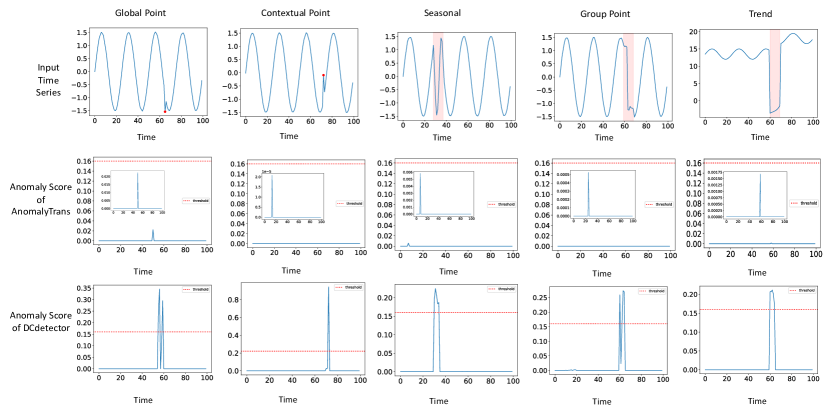
Figure 5. Visualization comparisons of ground-truth anomalies and anomaly scores between DCdetector and Anomaly Transformer for different types of anomalies.

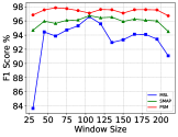
(a) Window size

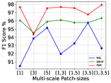
(b) Multi-scale size

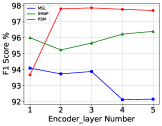
(c) Encoder layer number

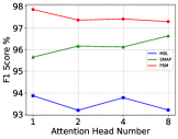
(d) Attention head number

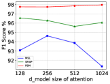
(e) $d_{model}$ of attention

Figure 6. Parameter sensitivity studies of main hyper-parameters in DCdetector.

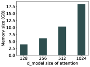
(a) Memory used

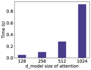
(b) Time cost

Figure 7. The averaged GPU memory cost and the averaged running time of 100 iterations during training with different $d_{model}$ sizes.

4.5.1. Ablation Studies

Table 6 shows the ablation study of stop gradient. According to the loss function definition in Section 3.3, we use two stop gradient modules in $\mathcal{L}\{\mathcal{P},\mathcal{N};\mathcal{X}\}$, noted as stop gradient in patch-wise branch and in-patch branch, respectively. With two-stop gradient modules, we can see that DCdetector gains the best performances. If no stop gradient is contained, DCdetector still works and does not fall into a trivial solution. Moreover, in such a setting, it outperforms all the baselines except Anomaly Transformer. Besides, we also conduct an ablation study on how the two main preprocessing methods (bilateral filter for denoising and instance normalization for normalization) affect the performance of our method in Table 7. It can be seen that either of them slightly improves the performance of our model when used individually. However, if they are utilized simultaneously, the performance degrades. Therefore, our final DCdetector only contains the instance normalization module for preprocessing. More ablation studies on multi-scale patching, window size, attention head, embedding dimension, encoder layer, anomaly threshold, and metrics in loss function are left in Appendix C.

4.5.2. Visual Analysis

We show how DCdetector works by visualizing different anomalies in Figure 5. We use the synthetic data generation methods reported in (Lai et al., 2021) to generate univariate time series with different types of anomalies, including point-wise anomalies (global point and contextual point anomalies) and pattern-wise anomalies (seasonal, group, and trend anomalies) (Lai et al., 2021). It can be seen that DCdetector can robustly detect various anomalies better from normal points with relatively higher anomaly scores.

4.5.3. Parameter Sensitivity

We also study the parameter sensitivity of the DCdetector. Figure 6(a) shows the performance under different window sizes. As discussed, a single point can not be taken as an instance in a time series. Window segmentation is widely used in the analysis, and window size is a significant parameter. For our primary evaluation, the window size is usually set as 60 or 100. Nevertheless, results in Figure 6(a) demonstrate that DCdetector is robust with a wide range of window sizes (from 30 to 210). Actually, in the window size range [45, 195], the performances fluctuate less than 2.3%. Figure 6(b) shows the performance under different multi-scale sizes. Horizontal coordinate is the patch-size combination used in multi-scale attention which means we combine several dual-attention modules with a given patch-size combination. Unlike window size, the multi-scale design contributes to the final performance of the DCdetector, and different patch-size combinations lead to different performances. Note that when studying the parameter sensitivity of window size, the scale size is fixed as [3,5]. When studying the parameter sensitivity of scale size, the window size is fixed at 60. Figure 6(c) shows the performance under different numbers of encoder layers, since many deep neural networks’ performances are affected by the layer number. Figure 6(d) and Figure 6(e) show model performances with different head numbers or $d_{model}$ sizes in attention. It can be seen that DCdetector achieves the best performance with a small attention head number and $d_{model}$ size. The memory and time usages with different $d_{model}$ sizes are shown in Figure 7. Based on Figure 7 and Figure 6(e), we set the dimension of the hidden state $d_{model}=256$ for the performance-complexity trade-off, and it can be seen that DCdetector can work quite well under $d_{model}=256$ with efficient running time and small memory consumption.

5. Conclusion

This paper proposes a novel algorithm named DCdetector for time-series anomaly detection. We design a contrastive learning-based dual-branch attention structure in DCdetector to learn a permutation invariant representation. Such representation enlarges the differences between normal points and anomalies, improving detection accuracy. Besides, two additional designs: multiscale and channel independence patching, are implemented to enhance the performance. Moreover, we propose a pure contrastive loss function without reconstruction error, which empirically proves the effectiveness of contrastive representation compared to the widely used reconstructive one. Lastly, extensive experiments show that DCdetector achieves the best or comparable performance on eight benchmark datasets compared to various state-of-the-art algorithms.

6. Acknowledgements

This work was supported by Alibaba Group through Alibaba Research Intern Program.

Appendix A Algorithms

Algorithm 1 DCdetector Outliner

⬇

from einops import rearrange

class DCdetector(nn.Module):

def __init__(self, win_size, enc_in, c_out, n_heads, d_model, e_layers, patch_size, channel, d_ff, dropout):

super(DCdetector, self).__init__()

self.patch_size = patch_size

self.channel = channel

self.win_size = win_size

# Patching List Embedding

self.embedding_patch_size = nn.ModuleList()

self.embedding_patch_num = nn.ModuleList()

for i, patchsize in enumerate(self.patch_size):

self.embedding_patch_size.append(DataEmbedding(patchsize, d_model, dropout))

self.embedding_patch_num.append(DataEmbedding(self.win_size//patchsize, d_model, dropout))

self.embedding_window_size = DataEmbedding(enc_in, d_model, dropout)

# Dual Attention Encoder

self.encoder = Encoder(

[AttentionLayer(

DAC_structure(win_size, patch_size, channel, False, attention_dropout=dropout, output_attention=output_attention),

d_model, patch_size, channel, n_heads, win_size)

for l in range(e_layers)

],norm_layer=torch.nn.LayerNorm(d_model))

def forward(self, x):

B, L, M = x.shape #Batch win_size channel

revin_layer = RevIN(num_features=M)

patch_wise_mean = [], in_patch_mean = []

x_ori = self.embedding_window_size(x)

# Instance Normalization Operation

x = revin_layer(x, ’norm’)

# Mutil-scale Patching Operation

for patch_index, patchsize in enumerate(self.patch_size):

x_patch_size = rearrange(x, ’b␣(n␣p)␣m␣->␣(b␣m)␣n␣p’, p = patchsize)

x_patch_num = rearrange(x, ’b␣(p␣n)␣m␣->␣(b␣m)␣p␣n’, p = patchsize)

x_patch_size = self.embedding_patch_size[patch_index](x_patch_size)

x_patch_num = self.embedding_patch_num[patch_index](x_patch_num)

patch_wise, in_patch = self.encoder(x_patch_size, x_patch_num, x_ori, patch_index)

patch_wise_mean.append(patch_wise)

in_patch_mean.append(in_patch)

return patch_wise_mean, in_patch_mean

Algorithm 2 Dual Attention Contrastive Structure

⬇

from einops import reduce, repeat

from math import sqrt

class DAC_structure(nn.Module):

def __init__(self, win_size, patch_size, channel, scale=None, attention_dropout=0.05):

super(DAC_structure, self).__init__()

self.scale = scale

self.dropout = nn.Dropout(attention_dropout)

self.window_size = win_size

self.patch_size = patch_size

self.channel = channel

def forward(self, queries_patch_size, queries_patch_num, keys_patch_size, keys_patch_num, values, patch_index, attn_mask):

# Patch-wise Representation

B, L, H, E = queries_patch_size.shape #batch_size*channel, patch_num, n_head, d_model/n_head

scale_patch_size = self.scale or 1. / sqrt(E)

scores_patch_size = torch.einsum("blhe,bshe->bhls", queries_patch_size, keys_patch_size) #batch*ch, nheads, p_num, p_num

attn_patch_size = scale_patch_size * scores_patch_size

series_patch_size = self.dropout(torch.softmax(attn_patch_size, dim=-1)) # B*D_model H N N

# In-patch Representation

B, L, H, E = queries_patch_num.shape #batch_size*channel, patch_size, n_head, d_model/n_head

scale_patch_num = self.scale or 1. / sqrt(E)

scores_patch_num = torch.einsum("blhe,bshe->bhls", queries_patch_num, keys_patch_num) #batch*ch, nheads, p_size, p_size

attn_patch_num = scale_patch_num * scores_patch_num

series_patch_num = self.dropout(torch.softmax(attn_patch_num, dim=-1)) # B*D_model H S S

# Upsampling

series_patch_size = repeat(series_patch_size, ’blmn->bl(m␣repeat_m)(n␣repeat_n)’, repeat_m=self.patch_size[patch_index], repeat_n=self.patch_size[patch_index])

series_patch_num = series_patch_num.repeat(1,1,self.window_size//self.patch_size[patch_index],self.window_size//self.patch_size[patch_index])

return series_patch_size, series_patch_num

Two main algorithms and their codes are presented as follows, the DCdetector Outliner (Algorithm 1) and the Dual Attention Contrastive Structure (Algorithm 2).

For the DCdetector Outliner (Algorithm 1), we use nn.ModuleList() in PyTorch (Paszke et al., 2019) to define multiple patching scales and perform embedding and dual attention operations for each set of patch sizes. After instance normalization, patch-wise encoders and in-patch encoders are calculated in the patch number $N$ dimension and the patch size $P$ dimension, respectively. Finally, we average the different patching scales to obtain the final patch-wise representation $\mathcal{N}$ and in-patch representation $\mathcal{P}$.

For the Dual Attention Contrastive Structure (Algorithm 2), we calculate patch-wise representation based on Eq.1 - Eq.3 and in-patch representation using Eq.4 - Eq.6, respectively. Finally, we apply different upsampling methods to make the shape of the two representations the same for subsequent comparison of representation discrepancy. Note that, we do not need to calculate the specific attention values, as only two representations are made and the attention weights can also be used as representations as well as improving the efficiency of the code. Besides, only a single patch scale of dual attention contrastive structure is shown here, which may suffer from information loss when upsampling is performed. However, the multi-patch scale will compensate for this issue, as shown in Algorithm 1.

Appendix B Dataset Description

We summarize the seven adopted benchmark datasets for evaluation in Table 8. These datasets include both univariate and multivariate time series scenarios with different types and anomaly ratios. MSL, SMAP, PSM, SMD, SWaT, NIPS-TS-SWAN, and NIPS-TS-GECCO are multivariate time series datasets. UCR is a univariate time series dataset.

Appendix C Extra Studies

To verify the sensitivity of the parameters in the proposed DCdetector, more ablation experiments are conducted in this part. We provide more detailed results here than those in Section 4.5.1. We also show the memory used as well as the iteration time spent during the training process.

C.1. Study on Metrics in Loss Function

We use different statistical distances to calculate the discrepancy between patch-wise representation and in-patch representation, and the results are shown in Table 9. The loss function proposed in Section 3.3 can get the SOTA performance in all benchmarks. Note that only using simple KL divergence, which is an asymmetrical loss function, we can still get a comparable result. However, for the Jensen-Shannon (JS) divergence, there is visible performance degradation, especially for the MSL benchmark.

C.2. Study on Multi-scale Patching

The multi-patching scale $\in\{[1],[3],[5],[1,3],[1,5],[3,5],[1,3,5]\}$ are tested. Patch size preference is for odd numbers to prevent information loss during upsampling. Generally, multi-scale design results in larger memory and different datasets have different best multi-patching scales. This is perhaps due to different information densities and anomaly types in different situations. The details of evaluation results are shown in Table 10.

C.3. Study on Window Size

Window size is a significant hyper-parameter in time series analysis. It is used to split time series into instances, as usually, a single point can not be considered as a sample. The results in Table 11 show that DCdetector is rather robust in different window sizes. Actually, in a large range [45, 195], the performances are slightly lower than the best ones for all benchmarks. Besides, we also test the impact of window size on memory cost and running time. The window size will affect the memory cost in a quadratic computational complexity way. So, the trade-off between slide window size and memory cost/running time is pretty important, especially for real-life scenarios. Fortunately, DCdetector can work optimally with a window size of less than 105 in all benchmarks, which greatly decreases the complexity of the model and its memory cost.

C.4. Study on Attention Head

Generally, multi-head attention is widely used in attention networks. We study the influence of attention head number $H$ in DCdetector. In general, the number of attention heads is even, so we set $H\in\{1,2,4,8\}$. Fortunately, with a small attention head number, as shown in Table 12, our model still achieves good performances (the best one or slightly lower than the best). Thus, DCdetector does not need a large memory when running.

C.5. Study on Embedding Dimension

The embedding dimension $d_{model}$ is another important parameter in the attention network. As a hyperparameter of the hidden channels, it may have impacts on model performance, memory cost, and running efficiency. We set $d_{model}\in\{128,256,512,1024\}$ as suggested hyperparameters by Transformer (Vaswani et al., 2017). For SMAP and PSM, it has little effect on the final results. As for MSL, it achieves the best performance with a small $d_{model}$ size and small memory. Overall, the proposed DCdetector can achieve quite good performance even with a small memory cost and good real-time performance. Details are in Table 13.

C.6. Study on Encoder Layer

Many deep models’ performances are dependent on the number of network layers $L$. We also show the influence of the number of encoder layers in Table 14. We set $L\in\{1,2,3,4,5\}$ as suggested hyperparameters by Transformer (Vaswani et al., 2017). Different benchmarks have different optimal parameters. Luckily, our model can gain the best performance in no more than 3 layers, and will not fail with too few encoder layers or over-fit with too many encoder layers.

C.7. Study on Anomaly Threshold

Anomaly threshold $\delta$ is a hyperparameter, which may affect the determination of anomaly or not, based on Eq. 12. We have a default value of 1 for all benchmarks. As shown in Table 15, when it is in the range of 0.5 to 1, it has little effect on the final model performance. PSM and SMAP are also more robust to anomaly threshold than MSL. For the three benchmarks, its best results appear when $\delta$ equals 0.7 or 0.8.

Table 8. Details of benchmark datasets. AR (anomaly ratio) represents the abnormal proportion of the whole dataset.

Benchmark	Source	Dimension	Window	Patch Size	#Training	#Test (Labeled)	AR (%)
MSL	NASA Space Sensors	55	90	[3,5]	58,317	73,729	10.5
SMAP	NASA Space Sensors	25	105	[3,5,7]	135,183	427,617	12.8
PSM	eBay Server Machine	25	60	[1,3,5]	132,481	87,841	27.8
SMD	Internet Server Machine	38	105	[5,7]	708,405	708,420	4.2
SWaT	Infrastructure System	51	105	[3,5,7]	495,000	449,919	12.1
NIPS-TS-SWAN	Space (Solar) Weather	38	36	[1,3]	60,000	60,000	32.6
NIPS-TS-GECCO	Water Quality for IoT	9	90	[1,3,5]	69,260	69,261	1.1
UCR	Various Natural Sources	1	105	[3,5,7]	2,238,349	6,143,541	0.6

Table 9. Ablation studies on metrics in the loss function. All results are in %. The best ones are in Bold.

Dataset	MSL			SMAP			PSM
Metric	P	R	F1	P	R	F1	P	R	F1
JS	89.23	70.42	78.72	93.23	93.62	93.42	97.18	92.29	94.67
Simple KL	92.44	98.82	95.52	92.20	93.44	92.82	97.80	96.71	97.25
DCdetector	93.69	99.69	96.60	95.63	98.92	97.02	97.14	98.74	97.94

Table 10. Ablation studies on multi-scale patching results (window size=60). All results are in %. The best ones are in Bold.

Dataset	MSL				SMAP				PSM				Mem (GB)	Time (s)
Metric	Acc	P	R	F1	Acc	P	R	F1	Acc	P	R	F1
Patch Size = [1]	97.98	92.77	88.29	90.48	98.96	93.91	98.31	96.06	98.82	97.27	98.07	97.66	16.9	0.42
Patch Size = [3]	98.64	92.39	95.34	93.84	98.59	94.65	94.43	94.54	97.22	96.95	91.84	94.33	6.0	0.24
Patch Size = [5]	98.91	92.55	97.87	95.14	98.92	94.40	97.44	95.90	98.75	97.22	97.84	97.53	3.2	0.17
Patch Size = [1,3]	98.30	93.19	90.77	91.96	98.98	94.42	97.87	96.11	98.83	96.96	98.42	97.68	16.9	0.59
Patch Size = [1,5]	98.52	92.88	93.60	93.24	98.89	94.15	97.49	95.79	98.76	97.03	98.07	97.55	16.9	0.46
Patch Size = [3,5]	98.93	93.88	97.72	95.76	98.89	94.61	96.95	95.77	98.38	97.00	96.54	96.77	6.0	0.27
Patch Size = [1,3,5]	98.44	91.52	93.78	92.64	99.03	93.72	99.10	96.34	98.95	97.14	98.74	97.94	16.9	0.71

Table 11. Ablation studies on window size results (patch size=[3,5]). All results are in %. The best ones are in Bold.

Dataset	MSL				SMAP				PSM				Mem (GB)	Time (s)
Metric	Acc	P	R	F1	Acc	P	R	F1	Acc	P	R	F1
Window size = 30	96.87	92.39	76.47	83.68	98.62	93.93	95.46	94.69	98.42	97.42	96.27	96.84	2.9	0.17
Window size = 45	98.77	92.80	96.13	94.44	98.94	94.24	97.75	95.96	98.79	97.01	98.09	97.55	6.0	0.22
Window size = 60	98.63	91.82	96.01	93.87	98.87	94.87	96.44	95.65	98.91	97.04	98.67	97.85	6.1	0.28
Window size = 75	98.79	91.71	97.93	94.72	98.97	94.62	97.60	96.09	98.79	97.26	98.20	97.73	7.6	0.36
Window size = 90	98.94	92.04	98.82	95.31	98.99	94.61	97.69	96.13	98.74	96.87	98.05	97.46	7.6	0.40
Window size = 105	99.06	93.69	99.69	96.60	99.16	94.69	98.87	96.74	98.57	96.84	97.37	97.10	18.5	0.46
Window size = 120	98.95	92.64	98.74	95.59	99.08	94.48	98.48	96.44	98.80	97.00	98.24	97.61	18.5	0.53
Window size = 135	98.44	91.52	94.45	92.96	99.09	94.26	98.91	96.53	98.70	96.97	98.17	97.57	24.4	0.60
Window size = 150	98.49	91.70	95.02	93.34	98.93	94.40	97.48	95.92	98.55	97.02	97.18	97.10	24.4	0.67
Window size = 165	98.64	92.61	95.68	94.12	99.01	94.50	98.07	96.25	98.77	97.11	98.05	97.58	24.4	0.74
Window size = 180	98.68	92.13	96.13	94.09	98.99	94.53	97.73	96.10	98.67	97.31	97.87	97.59	24.4	0.81
Window size = 195	98.50	92.68	94.18	93.43	98.95	94.44	97.60	96.00	98.66	97.24	97.88	97.55	24.5	0.89
Window size = 210	98.03	91.31	90.88	91.09	98.58	92.79	96.29	94.51	98.39	96.86	96.59	96.72	24.5	0.97

Table 12. Ablation studies on attention head $H$ results (patch size=[3,5], window size=60). All results are in %. The best ones are in Bold.

Dataset	MSL				SMAP				PSM				Mem (GB)	Time (s)
Metric	Acc	P	R	F1	Acc	P	R	F1	Acc	P	R	F1
$H$ = 1	98.63	91.82	96.01	93.87	98.87	94.87	96.44	95.65	98.91	97.04	98.67	97.85	6.1	0.05
$H$ = 2	98.50	92.13	94.29	93.20	98.98	93.99	98.44	96.16	98.67	97.16	97.55	97.36	6.1	0.17
$H$ = 4	98.67	91.93	95.71	93.78	98.97	93.89	98.46	96.12	98.69	97.02	97.79	97.41	9.8	0.19
$H$ = 8	98.55	91.30	95.21	93.21	99.11	94.87	98.47	96.63	98.63	96.84	97.73	97.29	9.8	0.40

Table 13. Ablation studies on embedding $d_{model}$ results (patch size=[3,5], window size=60). All results are in %. The best ones are in Bold.

Dataset	MSL				SMAP				PSM				Mem (GB)	Time (s)
Metric	Acc	P	R	F1	Acc	P	R	F1	Acc	P	R	F1
$d_{model}$ = 128	98.47	91.62	94.59	93.08	99.10	94.85	98.34	96.56	98.86	97.13	98.38	97.75	3.9	0.05
$d_{model}$ = 256	98.79	91.47	98.02	94.63	99.02	94.25	98.40	96.28	98.85	96.98	98.51	97.74	6.1	0.10
$d_{model}$ = 512	98.63	91.82	96.01	93.87	98.87	94.87	96.44	95.65	98.91	97.04	98.67	97.85	10.3	0.28
$d_{model}$ = 1024	98.13	91.92	90.81	91.36	98.97	94.87	97.27	96.06	98.97	97.11	98.83	97.96	18.4	0.92

Table 14. Ablation studies on encoder layers $L$ results (patch size=[3,5], window size=60). All results are in %. The best ones are in Bold.

Dataset	MSL				SMAP				PSM				Mem (GB)	Time (s)
Metric	Acc	P	R	F1	Acc	P	R	F1	Acc	P	R	F1
$L$ = 1	98.73	91.76	96.52	94.08	98.94	94.34	97.69	95.98	96.92	97.26	90.33	93.66	6.0	0.02
$L$ = 2	98.67	98.67	94.56	93.72	98.75	93.93	96.53	95.22	98.88	97.24	98.35	97.79	6.0	0.04
$L$ = 3	98.63	91.82	96.01	93.87	98.87	94.87	96.44	95.65	98.91	97.04	98.67	97.85	6.1	0.10
$L$ = 4	98.33	91.52	92.72	92.11	99.01	95.03	97.42	96.21	98.88	97.00	98.53	97.76	6.1	0.19
$L$ = 5	98.34	91.38	92.91	92.14	99.04	94.23	98.63	96.38	98.83	96.97	98.41	97.69	6.1	0.24

Table 15. Ablation studies on anomaly threshold $\delta$ results (patch size=[3,5], window size=60). All results are in %. The best ones are in Bold.

Dataset	MSL				SMAP				PSM
Metric	Acc	P	R	F1	Acc	P	R	F1	Acc	P	R	F1
$\delta$=0.5	96.62	95.69	72.23	82.32	98.85	96.60	94.40	95.49	98.45	98.76	95.03	96.86
$\delta$=0.6	98.08	94.75	87.20	90.80	99.12	96.66	96.53	96.59	98.71	98.27	96.56	97.41
$\delta$=0.7	98.80	93.65	95.47	94.55	99.29	95.73	98.88	97.28	98.98	98.14	97.81	97.97
$\delta$=0.8	98.83	93.12	96.40	94.73	99.06	94.29	98.72	96.45	98.88	97.71	97.85	97.78
$\delta$=0.9	98.42	91.90	93.75	92.82	98.82	93.81	97.32	95.54	98.92	97.42	98.31	97.86
$\delta$=1.0	98.33	92.58	92.04	92.31	98.90	93.30	98.56	95.86	98.91	97.04	98.67	97.85

References

- (1)
- Abdulaal et al. (2021) Ahmed Abdulaal, Zhuanghua Liu, and Tomer Lancewicki. 2021. Practical approach to asynchronous multivariate time series anomaly detection and localization. In Proceedings of the 27th ACM SIGKDD Conference on Knowledge Discovery & Data Mining. 2485–2494.
- Adams and MacKay (2007) Ryan Prescott Adams and David JC MacKay. 2007. Bayesian online changepoint detection. arXiv preprint arXiv:0710.3742 (2007).
- Anandakrishnan et al. (2018) Archana Anandakrishnan, Senthil Kumar, Alexander Statnikov, Tanveer Faruquie, and Di Xu. 2018. Anomaly detection in finance: editors’ introduction. In KDD 2017 Workshop on Anomaly Detection in Finance. PMLR, 1–7.
- Anderson (1976) OD Anderson. 1976. Time-Series. 2nd edn.
- Angryk et al. (2020) Rafal Angryk, Petrus Martens, Berkay Aydin, Dustin Kempton, Sushant Mahajan, Sunitha Basodi, Azim Ahmadzadeh, Xumin Cai, Soukaina Filali Boubrahimi, Shah Muhammad Hamdi, Micheal Schuh, and Manolis Georgoulis. 2020. SWAN-SF. https://doi.org/10.7910/DVN/EBCFKM
- Blázquez-García et al. (2021) Ane Blázquez-García, Angel Conde, Usue Mori, and Jose A Lozano. 2021. A review on outlier/anomaly detection in time series data. ACM Computing Surveys (CSUR) 54, 3 (2021), 1–33.
- Boniol and Palpanas (2020) Paul Boniol and Themis Palpanas. 2020. Series2Graph: Graph-based Subsequence Anomaly Detection for Time Series. ArXiv abs/2207.12208 (2020).
- Bontemps et al. (2016) Loïc Bontemps, Van Loi Cao, James McDermott, and Nhien-An Le-Khac. 2016. Collective anomaly detection based on long short-term memory recurrent neural networks. In International conference on future data and security engineering. Springer, 141–152.
- Box and Pierce (1970) George EP Box and David A Pierce. 1970. Distribution of residual autocorrelations in autoregressive-integrated moving average time series models. Journal of the American statistical Association 65, 332 (1970), 1509–1526.
- Breunig et al. (2000) Markus M Breunig, Hans-Peter Kriegel, Raymond T Ng, and Jörg Sander. 2000. LOF: identifying density-based local outliers. In Proceedings of the 2000 ACM SIGMOD international conference on Management of data. 93–104.
- Campos et al. (2021) David Campos, Tung Kieu, Chenjuan Guo, Feiteng Huang, Kai Zheng, Bin Yang, and Christian S Jensen. 2021. Unsupervised Time Series Outlier Detection with Diversity-Driven Convolutional Ensembles–Extended Version. arXiv preprint arXiv:2111.11108 (2021).
- Canizo et al. (2019) Mikel Canizo, Isaac Triguero, Angel Conde, and Enrique Onieva. 2019. Multi-head CNN–RNN for multi-time series anomaly detection: An industrial case study. Neurocomputing 363 (2019), 246–260.
- Caron et al. (2020) Mathilde Caron, Ishan Misra, Julien Mairal, Priya Goyal, Piotr Bojanowski, and Armand Joulin. 2020. Unsupervised learning of visual features by contrasting cluster assignments. Advances in neural information processing systems 33 (2020), 9912–9924.
- Chauhan and Vig (2015) Sucheta Chauhan and Lovekesh Vig. 2015. Anomaly detection in ECG time signals via deep long short-term memory networks. In 2015 IEEE international conference on data science and advanced analytics (DSAA). IEEE, 1–7.
- Chen et al. (2020) Ting Chen, Simon Kornblith, Mohammad Norouzi, and Geoffrey Hinton. 2020. A simple framework for contrastive learning of visual representations. In International conference on machine learning. PMLR, 1597–1607.
- Chen et al. (2021b) Xuanhao Chen, Liwei Deng, Feiteng Huang, Chengwei Zhang, Zongquan Zhang, Yan Zhao, and Kai Zheng. 2021b. Daemon: Unsupervised anomaly detection and interpretation for multivariate time series. In 2021 IEEE 37th International Conference on Data Engineering (ICDE). IEEE, 2225–2230.
- Chen and He (2021) Xinlei Chen and Kaiming He. 2021. Exploring simple siamese representation learning. In Proceedings of the IEEE/CVF Conference on Computer Vision and Pattern Recognition. 15750–15758.
- Chen et al. (2021a) Zekai Chen, Dingshuo Chen, Xiao Zhang, Zixuan Yuan, and Xiuzhen Cheng. 2021a. Learning graph structures with transformer for multivariate time-series anomaly detection in IoT. IEEE Internet of Things Journal 9, 12 (2021), 9179–9189.
- Cheng et al. (2009) Haibin Cheng, Pang-Ning Tan, Christopher Potter, and Steven Klooster. 2009. Detection and characterization of anomalies in multivariate time series. In Proceedings of the 2009 SIAM international conference on data mining. SIAM, 413–424.
- Cook et al. (2019) Andrew A Cook, Göksel Mısırlı, and Zhong Fan. 2019. Anomaly detection for IoT time-series data: A survey. IEEE Internet of Things Journal 7, 7 (2019), 6481–6494.
- Dau et al. (2019) Hoang Anh Dau, Anthony Bagnall, Kaveh Kamgar, Chin-Chia Michael Yeh, Yan Zhu, Shaghayegh Gharghabi, Chotirat Ann Ratanamahatana, and Eamonn Keogh. 2019. The UCR time series archive. IEEE/CAA Journal of Automatica Sinica 6, 6 (2019), 1293–1305.
- Deldari et al. (2021) Shohreh Deldari, Daniel V Smith, Hao Xue, and Flora D Salim. 2021. Time series change point detection with self-supervised contrastive predictive coding. In Proceedings of the Web Conference 2021. 3124–3135.
- Deng and Hooi (2021a) Ailin Deng and Bryan Hooi. 2021a. Graph Neural Network-Based Anomaly Detection in Multivariate Time Series. In AAAI Conference on Artificial Intelligence.
- Deng and Hooi (2021b) Ailin Deng and Bryan Hooi. 2021b. Graph neural network-based anomaly detection in multivariate time series. In Proceedings of the AAAI conference on artificial intelligence, Vol. 35. 4027–4035.
- Elsayed et al. (2021) Shereen Elsayed, Daniela Thyssens, Ahmed Rashed, Hadi Samer Jomaa, and Lars Schmidt-Thieme. 2021. Do we really need deep learning models for time series forecasting? arXiv preprint arXiv:2101.02118 (2021).
- Gao et al. (2020) Jingkun Gao, Xiaomin Song, Qingsong Wen, Pichao Wang, Liang Sun, and Huan Xu. 2020. RobustTAD: Robust time series anomaly detection via decomposition and convolutional neural networks. KDD Workshop MileTS (2020).
- Golmohammadi and Zaiane (2015) Koosha Golmohammadi and Osmar R Zaiane. 2015. Time series contextual anomaly detection for detecting market manipulation in stock market. In 2015 IEEE international conference on data science and advanced analytics (DSAA). IEEE, 1–10.
- Grill et al. (2020) Jean-Bastien Grill, Florian Strub, Florent Altché, Corentin Tallec, Pierre Richemond, Elena Buchatskaya, Carl Doersch, Bernardo Avila Pires, Zhaohan Guo, Mohammad Gheshlaghi Azar, et al. 2020. Bootstrap your own latent-a new approach to self-supervised learning. Advances in neural information processing systems 33 (2020), 21271–21284.
- He et al. (2020) Kaiming He, Haoqi Fan, Yuxin Wu, Saining Xie, and Ross Girshick. 2020. Momentum contrast for unsupervised visual representation learning. In Proceedings of the IEEE/CVF conference on computer vision and pattern recognition. 9729–9738.
- Huang et al. (2018) Chengqiang Huang, Yulei Wu, Yuan Zuo, Ke Pei, and Geyong Min. 2018. Towards experienced anomaly detector through reinforcement learning. In Proceedings of the AAAI Conference on Artificial Intelligence, Vol. 32.
- Huet et al. (2022) Alexis Huet, Jose Manuel Navarro, and Dario Rossi. 2022. Local Evaluation of Time Series Anomaly Detection Algorithms. In Proceedings of the 28th ACM SIGKDD Conference on Knowledge Discovery and Data Mining. 635–645.
- Hundman et al. (2018) Kyle Hundman, Valentino Constantinou, Christopher Laporte, Ian Colwell, and Tom Soderstrom. 2018. Detecting spacecraft anomalies using lstms and nonparametric dynamic thresholding. In Proceedings of the 24th ACM SIGKDD international conference on knowledge discovery & data mining. 387–395.
- Jiao et al. (2022) Yang Jiao, Kai Yang, Dongjing Song, and Dacheng Tao. 2022. Timeautoad: Autonomous anomaly detection with self-supervised contrastive loss for multivariate time series. IEEE Transactions on Network Science and Engineering 9, 3 (2022), 1604–1619.
- Kant and Mahajan (2019) Neha Kant and Manish Mahajan. 2019. Time-series outlier detection using enhanced k-means in combination with pso algorithm. In Engineering Vibration, Communication and Information Processing: ICoEVCI 2018, India. Springer, 363–373.
- Karczmarek et al. (2020) Paweł Karczmarek, Adam Kiersztyn, Witold Pedrycz, and Ebru Al. 2020. K-Means-based isolation forest. Knowledge-based systems 195 (2020), 105659.
- Keogh et al. (2021) Eamonn Keogh, Dutta Roy Taposh, U Naik, and A Agrawal. 2021. Multi-dataset Time-Series Anomaly Detection Competition. In ACM SIGKDD International Conference on Knowledge Discovery and Data Mining. https://compete. hexagonml. com/practice/competition/39.
- Khan et al. (2022) Adnan Khan, Sarah AlBarri, and Muhammad Arslan Manzoor. 2022. Contrastive self-supervised learning: a survey on different architectures. In 2022 2nd International Conference on Artificial Intelligence (ICAI). IEEE, 1–6.
- Kim et al. (2021) Taesung Kim, Jinhee Kim, Yunwon Tae, Cheonbok Park, Jang-Ho Choi, and Jaegul Choo. 2021. Reversible instance normalization for accurate time-series forecasting against distribution shift. In International Conference on Learning Representations.
- Kingma and Ba (2014) Diederik P Kingma and Jimmy Ba. 2014. Adam: A method for stochastic optimization. arXiv preprint arXiv:1412.6980 (2014).
- Lai et al. (2021) Kwei-Herng Lai, Daochen Zha, Junjie Xu, Yue Zhao, Guanchu Wang, and Xia Hu. 2021. Revisiting time series outlier detection: Definitions and benchmarks. In Thirty-fifth Conference on Neural Information Processing Systems Datasets and Benchmarks Track (Round 1).
- Li et al. (2019a) Dan Li, Dacheng Chen, Baihong Jin, Lei Shi, Jonathan Goh, and See-Kiong Ng. 2019a. MAD-GAN: Multivariate anomaly detection for time series data with generative adversarial networks. In Artificial Neural Networks and Machine Learning–ICANN 2019: Text and Time Series: 28th International Conference on Artificial Neural Networks, Munich, Germany, September 17–19, 2019, Proceedings, Part IV. Springer, 703–716.
- Li et al. (2022) Longyuan Li, Junchi Yan, Qingsong Wen, Yaohui Jin, and Xiaokang Yang. 2022. Learning robust deep state space for unsupervised anomaly detection in contaminated time-series. IEEE Transactions on Knowledge and Data Engineering (2022).
- Li et al. (2019b) Shiyang Li, Xiaoyong Jin, Yao Xuan, Xiyou Zhou, Wenhu Chen, Yu-Xiang Wang, and Xifeng Yan. 2019b. Enhancing the locality and breaking the memory bottleneck of transformer on time series forecasting. Advances in neural information processing systems 32 (2019).
- Li et al. (2021a) Xing Li, Qiquan Shi, Gang Hu, Lei Chen, Hui Mao, Yiyuan Yang, Mingxuan Yuan, Jia Zeng, and Zhuo Cheng. 2021a. Block Access Pattern Discovery via Compressed Full Tensor Transformer. In Proceedings of the 30th ACM International Conference on Information & Knowledge Management. 957–966.
- Li et al. (2021b) Zhihan Li, Youjian Zhao, Jiaqi Han, Ya Su, Rui Jiao, Xidao Wen, and Dan Pei. 2021b. Multivariate time series anomaly detection and interpretation using hierarchical inter-metric and temporal embedding. In Proceedings of the 27th ACM SIGKDD Conference on Knowledge Discovery & Data Mining. 3220–3230.
- Liu et al. (2008) Fei Tony Liu, Kai Ming Ting, and Zhi-Hua Zhou. 2008. Isolation forest. In 2008 eighth ieee international conference on data mining. IEEE, 413–422.
- Mathur and Tippenhauer (2016) Aditya P Mathur and Nils Ole Tippenhauer. 2016. SWaT: A water treatment testbed for research and training on ICS security. In 2016 international workshop on cyber-physical systems for smart water networks (CySWater). IEEE, 31–36.
- Moritz et al. (2018) Steffen Moritz, Frederik Rehbach, Sowmya Chandrasekaran, Margarita Rebolledo, and Thomas Bartz-Beielstein. 2018. GECCO Industrial Challenge 2018 Dataset: a water quality dataset for the “Internet of Things: Online Anomaly Detection for Drinking Water Quality” competition at the Genetic and Evolutionary Computation Conference 2018, Kyoto, Japan (2018).
- Munir et al. (2018) Mohsin Munir, Shoaib Ahmed Siddiqui, Andreas Dengel, and Sheraz Ahmed. 2018. DeepAnT: A deep learning approach for unsupervised anomaly detection in time series. Ieee Access 7 (2018), 1991–2005.
- Nie et al. (2022) Yuqi Nie, Nam H Nguyen, Phanwadee Sinthong, and Jayant Kalagnanam. 2022. A Time Series is Worth 64 Words: Long-term Forecasting with Transformers. arXiv preprint arXiv:2211.14730 (2022).
- Niu et al. (2020) Zijian Niu, Ke Yu, and Xiaofei Wu. 2020. LSTM-based VAE-GAN for time-series anomaly detection. Sensors 20, 13 (2020), 3738.
- Paparrizos et al. (2022) John Paparrizos, Paul Boniol, Themis Palpanas, Ruey S Tsay, Aaron Elmore, and Michael J Franklin. 2022. Volume under the surface: a new accuracy evaluation measure for time-series anomaly detection. Proceedings of the VLDB Endowment 15, 11 (2022), 2774–2787.
- Park et al. (2018) Daehyung Park, Yuuna Hoshi, and Charles C Kemp. 2018. A multimodal anomaly detector for robot-assisted feeding using an lstm-based variational autoencoder. IEEE Robotics and Automation Letters 3, 3 (2018), 1544–1551.
- Paszke et al. (2019) Adam Paszke, Sam Gross, Francisco Massa, Adam Lerer, James Bradbury, Gregory Chanan, Trevor Killeen, Zeming Lin, Natalia Gimelshein, Luca Antiga, et al. 2019. Pytorch: An imperative style, high-performance deep learning library. Advances in neural information processing systems 32 (2019).
- Perslev et al. (2019) Mathias Perslev, Michael Jensen, Sune Darkner, Poul Jørgen Jennum, and Christian Igel. 2019. U-time: A fully convolutional network for time series segmentation applied to sleep staging. Advances in Neural Information Processing Systems 32 (2019).
- Phillips and Jin (2015) Peter CB Phillips and Sainan Jin. 2015. Business cycles, trend elimination, and the HP filter. (2015).
- Ren et al. (2019) Hansheng Ren, Bixiong Xu, Yujing Wang, Chao Yi, Congrui Huang, Xiaoyu Kou, Tony Xing, Mao Yang, Jie Tong, and Qi Zhang. 2019. Time-series anomaly detection service at microsoft. In Proceedings of the 25th ACM SIGKDD international conference on knowledge discovery & data mining. 3009–3017.
- Rousseeuw and Leroy (2005) Peter J Rousseeuw and Annick M Leroy. 2005. Robust regression and outlier detection. John wiley & sons.
- Ruff et al. (2021) Lukas Ruff, Jacob R Kauffmann, Robert A Vandermeulen, Grégoire Montavon, Wojciech Samek, Marius Kloft, Thomas G Dietterich, and Klaus-Robert Müller. 2021. A unifying review of deep and shallow anomaly detection. Proc. IEEE 109, 5 (2021), 756–795.
- Ruff et al. (2018) Lukas Ruff, Robert Vandermeulen, Nico Goernitz, Lucas Deecke, Shoaib Ahmed Siddiqui, Alexander Binder, Emmanuel Müller, and Marius Kloft. 2018. Deep one-class classification. In International conference on machine learning. PMLR, 4393–4402.
- Sakurada and Yairi (2014) Mayu Sakurada and Takehisa Yairi. 2014. Anomaly detection using autoencoders with nonlinear dimensionality reduction. In Proceedings of the MLSDA 2014 2nd workshop on machine learning for sensory data analysis. 4–11.
- Salinas et al. (2020) David Salinas, Valentin Flunkert, Jan Gasthaus, and Tim Januschowski. 2020. DeepAR: Probabilistic forecasting with autoregressive recurrent networks. International Journal of Forecasting 36, 3 (2020), 1181–1191.
- Schmidl et al. (2022) Sebastian Schmidl, Phillip Wenig, and Thorsten Papenbrock. 2022. Anomaly detection in time series: a comprehensive evaluation. Proceedings of the VLDB Endowment 15, 9 (2022), 1779–1797.
- Shen et al. (2020) Lifeng Shen, Zhuocong Li, and James Kwok. 2020. Timeseries anomaly detection using temporal hierarchical one-class network. Advances in Neural Information Processing Systems 33 (2020), 13016–13026.
- Shin et al. (2020) Youjin Shin, Sangyup Lee, Shahroz Tariq, Myeong Shin Lee, Okchul Jung, Daewon Chung, and Simon S Woo. 2020. Itad: integrative tensor-based anomaly detection system for reducing false positives of satellite systems. In Proceedings of the 29th ACM international conference on information & knowledge management. 2733–2740.
- Su et al. (2019) Ya Su, Youjian Zhao, Chenhao Niu, Rong Liu, Wei Sun, and Dan Pei. 2019. Robust anomaly detection for multivariate time series through stochastic recurrent neural network. In Proceedings of the 25th ACM SIGKDD international conference on knowledge discovery & data mining. 2828–2837.
- Tariq et al. (2019) Shahroz Tariq, Sangyup Lee, Youjin Shin, Myeong Shin Lee, Okchul Jung, Daewon Chung, and Simon S Woo. 2019. Detecting anomalies in space using multivariate convolutional LSTM with mixtures of probabilistic PCA. In Proceedings of the 25th ACM SIGKDD international conference on knowledge discovery & data mining. 2123–2133.
- Tax and Duin (2004) David MJ Tax and Robert PW Duin. 2004. Support vector data description. Machine learning 54, 1 (2004), 45–66.
- Ulyanov et al. (2017) Dmitry Ulyanov, Andrea Vedaldi, and Victor Lempitsky. 2017. Improved texture networks: Maximizing quality and diversity in feed-forward stylization and texture synthesis. In Proceedings of the IEEE conference on computer vision and pattern recognition. 6924–6932.
- Vaswani et al. (2017) Ashish Vaswani, Noam Shazeer, Niki Parmar, Jakob Uszkoreit, Llion Jones, Aidan N Gomez, Łukasz Kaiser, and Illia Polosukhin. 2017. Attention is all you need. Advances in neural information processing systems 30 (2017).
- Wen et al. (2022) Qingsong Wen, Linxiao Yang, Tian Zhou, and Liang Sun. 2022. Robust time series analysis and applications: An industrial perspective. In Proceedings of the 28th ACM SIGKDD Conference on Knowledge Discovery and Data Mining. 4836–4837.
- Wu et al. (2021) Haixu Wu, Jiehui Xu, Jianmin Wang, and Mingsheng Long. 2021. Autoformer: Decomposition transformers with auto-correlation for long-term series forecasting. Advances in Neural Information Processing Systems 34 (2021), 22419–22430.
- Wu et al. (2018) Zhirong Wu, Yuanjun Xiong, Stella X Yu, and Dahua Lin. 2018. Unsupervised feature learning via non-parametric instance discrimination. In Proceedings of the IEEE conference on computer vision and pattern recognition. 3733–3742.
- Xu et al. (2018) Haowen Xu, Wenxiao Chen, Nengwen Zhao, Zeyan Li, Jiahao Bu, Zhihan Li, Ying Liu, Youjian Zhao, Dan Pei, Yang Feng, et al. 2018. Unsupervised anomaly detection via variational auto-encoder for seasonal kpis in web applications. In Proceedings of the 2018 world wide web conference. 187–196.
- Xu et al. (2021) Jiehui Xu, Haixu Wu, Jianmin Wang, and Mingsheng Long. 2021. Anomaly transformer: Time series anomaly detection with association discrepancy. arXiv preprint arXiv:2110.02642 (2021).
- Yairi et al. (2017) Takehisa Yairi, Naoya Takeishi, Tetsuo Oda, Yuta Nakajima, Naoki Nishimura, and Noboru Takata. 2017. A data-driven health monitoring method for satellite housekeeping data based on probabilistic clustering and dimensionality reduction. IEEE Trans. Aerospace Electron. Systems 53, 3 (2017), 1384–1401.
- Yang et al. (2023) Yiyuan Yang, Rongshang Li, Qiquan Shi, Xijun Li, Gang Hu, Xing Li, and Mingxuan Yuan. 2023. SGDP: A Stream-Graph Neural Network Based Data Prefetcher. arXiv preprint arXiv:2304.03864 (2023).
- Yang et al. (2021a) Yiyuan Yang, Yi Li, and Haifeng Zhang. 2021a. Pipeline safety early warning method for distributed signal using bilinear CNN and LightGBM. In ICASSP 2021-2021 IEEE International Conference on Acoustics, Speech and Signal Processing (ICASSP). IEEE, 4110–4114.
- Yang et al. (2021b) Yiyuan Yang, Yi Li, Taojia Zhang, Yan Zhou, and Haifeng Zhang. 2021b. Early safety warnings for long-distance pipelines: A distributed optical fiber sensor machine learning approach. In Proceedings of the AAAI Conference on Artificial Intelligence, Vol. 35. 14991–14999.
- Yang et al. (2021c) Yiyuan Yang, Haifeng Zhang, and Yi Li. 2021c. Long-distance pipeline safety early warning: a distributed optical fiber sensing semi-supervised learning method. IEEE Sensors Journal 21, 17 (2021), 19453–19461.
- Yang et al. (2021d) Yiyuan Yang, Haifeng Zhang, and Yi Li. 2021d. Pipeline safety early warning by multifeature-fusion CNN and LightGBM analysis of signals from distributed optical fiber sensors. IEEE Transactions on Instrumentation and Measurement 70 (2021), 1–13.
- Ye et al. (2019) Mang Ye, Xu Zhang, Pong C Yuen, and Shih-Fu Chang. 2019. Unsupervised embedding learning via invariant and spreading instance feature. In Proceedings of the IEEE/CVF Conference on Computer Vision and Pattern Recognition. 6210–6219.
- Yeh et al. (2016) Chin-Chia Michael Yeh, Yan Zhu, Liudmila Ulanova, Nurjahan Begum, Yifei Ding, Hoang Anh Dau, Diego Furtado Silva, Abdullah Mueen, and Eamonn Keogh. 2016. Matrix profile I: all pairs similarity joins for time series: a unifying view that includes motifs, discords and shapelets. In 2016 IEEE 16th international conference on data mining (ICDM). Ieee, 1317–1322.
- Yu and Sun (2020) Mengran Yu and Shiliang Sun. 2020. Policy-based reinforcement learning for time series anomaly detection. Engineering Applications of Artificial Intelligence 95 (2020), 103919.
- Zamanzadeh Darban et al. (2022) Zahra Zamanzadeh Darban, Geoffrey I Webb, Shirui Pan, Charu C Aggarwal, and Mahsa Salehi. 2022. Deep Learning for Time Series Anomaly Detection: A Survey. arXiv e-prints (2022), arXiv–2211.
- Zhang et al. (2022b) Chaoning Zhang, Kang Zhang, Chenshuang Zhang, Trung X Pham, Chang D Yoo, and In So Kweon. 2022b. How does SimSiam avoid collapse without negative samples? a unified understanding with self-supervised contrastive learning. Proceedings of International Conference on Learning Representations (ICLR) (2022).
- Zhang et al. (2022c) Chaoli Zhang, Tian Zhou, Qingsong Wen, and Liang Sun. 2022c. TFAD: A Decomposition Time Series Anomaly Detection Architecture with Time-Frequency Analysis. In Proceedings of the 31st ACM International Conference on Information & Knowledge Management. 2497–2507.
- Zhang et al. (2022a) Yuxin Zhang, Jindong Wang, Yiqiang Chen, Han Yu, and Tao Qin. 2022a. Adaptive memory networks with self-supervised learning for unsupervised anomaly detection. IEEE Transactions on Knowledge and Data Engineering (2022).
- Zhao et al. (2020a) Hang Zhao, Yujing Wang, Juanyong Duan, Congrui Huang, Defu Cao, Yunhai Tong, Bixiong Xu, Jing Bai, Jie Tong, and Qi Zhang. 2020a. Multivariate Time-series Anomaly Detection via Graph Attention Network. 2020 IEEE International Conference on Data Mining (ICDM) (2020), 841–850.
- Zhao et al. (2020b) Hang Zhao, Yujing Wang, Juanyong Duan, Congrui Huang, Defu Cao, Yunhai Tong, Bixiong Xu, Jing Bai, Jie Tong, and Qi Zhang. 2020b. Multivariate time-series anomaly detection via graph attention network. In 2020 IEEE International Conference on Data Mining (ICDM). IEEE, 841–850.
- Zhou et al. (2019) Bin Zhou, Shenghua Liu, Bryan Hooi, Xueqi Cheng, and Jing Ye. 2019. BeatGAN: Anomalous Rhythm Detection using Adversarially Generated Time Series.. In IJCAI, Vol. 2019. 4433–4439.
- Zong et al. (2018) Bo Zong, Qi Song, Martin Renqiang Min, Wei Cheng, Cristian Lumezanu, Daeki Cho, and Haifeng Chen. 2018. Deep autoencoding gaussian mixture model for unsupervised anomaly detection. In International conference on learning representations.