Collapsing molecular clouds with tracer particles: II. Collapse Histories.

Abstract

In order to develop a complete theory of star formation, one essentially needs to know two things: what collapses, and how long it takes. This is the second paper in a series, where we query how long a parcel of gas takes to collapse and the process it undergoes. We embed pseudo-Lagrangian tracer particles in simulations of collapsing molecular clouds, identify the particles that end in dense knots, and then examine the collapse history of the gas. We find a nearly universal behavior of cruise-then-collapse. We identify gas the moment before it collapses, $t_{\rm{sing}}$, and examine how it transitions to high density. We find that the time to collapse is uniformly distributed between $0.25t_{\rm{ff}}$ and the end of the simulation at $\sim 1t_{\rm{ff}}$, and that the collapse duration is universally short, $\Delta t\sim 0.1t_{\rm{ff}}$. We find that the collapse of each core happens by a process akin to violent relaxation, wherein a fast reordering of the potential and kinetic energies occurs, in $0.1t_{\rm{ff}}$, after which a virialized object remains. We describe the collapse in four stages; collection, hardening, singularity, and mosh. Collection sweeps low density gas into moderate density. Hardening brings kinetic and gravitational energies into quasi-equipartition. Singularity is the free-fall collapse, forming a virialized object in $\sim 0.1\tff$. Mosh encompasses tidal dynamics of sub clumps and nearby cores during the collapse. In this work we focus primarily on isolated clumps. With this novel lens we can observe the details of collapse.

1 Introduction

Stars form from clouds of hydrogen that are cold (T=10K) low density ($n=100$ ), turbulent ($\sigma_{v}=few\times c_{s}$) and magnetized (Solomon et al., 1987; Crutcher, 2012; Miville-Deschênes et al., 2017). Prestellar cores are denser and more magnetized (Crutcher, 2012) objects that are often associated with embedded infrared sources. It appears that a population of these cores are coherent, meaning sub- or trans-virial (Goodman et al., 1998; Singh et al., 2021; Choudhury et al., 2021). The mass distributions of cores (Ladjelate et al., 2020) and the initial mass function (Chabrier, 2003) are similar in shape but offset by a factor of $\epsilon=3-4$. This indicates that cores are related to the formation of stars, with a fraction of each core, $1/\epsilon$, given to each star (Alves et al., 2007).

Many models and computer simulations have been devised to describe these processes. Early models had magnetic fields regulating the collapse by slowing the gravitational contraction (e.g. Shu et al., 1987; Mouschovias, 1987), but these models were largely ruled out by observations (Crutcher et al., 2009). Many modern turbulent fragmentation models are based on Padoan (1995), wherein some subset of the lognormal density PDF is turned into stars (Krumholz & McKee, 2005; Hennebelle & Chabrier, 2011; Padoan & Nordlund, 2011), though the physics behind these models is different from one another. More recent models include the inertial flow model (Pelkonen et al., 2021), where large scale flow drives core formation, and the three phase model of Offner et al. (2022), wherein turbulence gives way to coherent structures. Our simulation set up and outcomes are similar to these, with a few notable differences due to the novel way in which we examine the collapse.

This is the second paper in a series wherein we inject pseudo-Lagrangian tracer particles in a simulation of turbulent, collapsing molecular clouds. We allow the cloud to collapse to form several hundred prestellar cores, identify the particles in those cores, and then examine the cells that those particles occupy during the collapse. At all times prior to the end of the simulation, we refer to zones that contain core particles as preimage gas. In the first paper (Collins et al., 2023), we examine the preimage gas at $t=0$, the beginning of the simulation. We find that the density PDF is fully covered by the PDF of the preimage gas, but suppressed by a factor of roughly $\rho^{1/2}$: all gas participates in the collapse, dense gas preferentially. We find that gas is distributed in a fractal manner, with a typical fractal dimension of 1.6. We also find a high degree of overlap of the primage gas between different cores. Cores that are close to one another at the end of the simulation, e.g. binaries, come from gas that seems to be mixed in the initial cloud. We also examine length scales of both density and velocity. We find that the length scale of the preimage gas is several times larger than the density auto correlation length, indicating that many density fluctuations in the initial parent cloud contribute to each core in a many-to-many fashion. We find that the length scale of the preimage gas is comparable to the velocity correlation length, indicating one or a few large scale flows dictate the collapse.

In this work, we examine the time history of collapsing gas. We use the same simulations described in Collins et al. (2023), but now follow them beyond $t=0$. In this work we focus on the collapse of isolated cores. In future installations of the series we will discuss magnetic fields, binaries, and clusters.

The paper is organized as follows. In Section 2 we discuss the code, simulations, and particle identification. Results are presented in Section 1. We begin by separating cores by their clustering (alone, binary, or cluster) in Section 3.1. This is necessary to isolate collapse (which we are primarily interested in) from tidal effects (which we are also interested in, but is much more complex). In Section 3.2 we discuss the collapse time, , and its distribution. We discuss the unexpected lack of correlation between  and mean quantities of the preimage gas in 3.3. Section 3.4 follows in detail the collapse of a fiducial object, and we discuss three of the four stages of collapse (collection, hardening, and singularity). We then show the stacked mean density and velocity tracks for a large population of cores in Section 3.5, stretched to each cores’ collapse time, and show the nearly universal transition to coherence, followed by free-fall collapse. Radial profiles are shown in Section 3.5.3, which most clearly show rapid virialization. Binaries, clusters, and the fourth stage, mosh, are discussed in Section 3.6. We summarize and discuss in Section 4.

2 Method: Code and Cores

This work uses the simulations and methods described in detail in Collins et al. (2023). We will briefly recap the code, simulations, and particle methods here.

2.1 Code

We use the open source Adaptive Mesh Refinement (AMR) code Enzo (Bryan et al., 2014) with the constrained transport (CT) magnetohydrodynamics module (Collins et al., 2010). This code adaptively adds resolution as the collapse unfolds, when the local Jeans length $L_{J}=\sqrt{3\pi/32G\rho_{0}}$ exceeds 16 zones. The main solver is a higher order Godunov method, using the linear method of Li et al. (2008) for the differential equations, the HLLD method of Mignone (2007), and the electric field defined by Gardiner & Stone (2005) to maintain the divergence of the magnetic field. The code adaptively adds zones using the methods of Berger & Colella (1989) and Balsara (2001). It has been demonstrated to preserve the divergence of the magnetic field to machine precision (Collins et al., 2010), and has been used in a wide array of applications from star formation (Collins et al., 2011) to galaxy clusters (Xu et al., 2012; Skillman et al., 2013). We additionally include tracer particles that follow the flow by way of a piecewise linear interpolation of the velocity field (see Bryan et al., 2014; Collins et al., 2023, for a description).

We do not use sink particles in this work. This choice was made so that we can see the details of the collapse without the influence of a subgrid model. This limits the duration of the simulation.

2.2 Simulations

The simulations are first stirred in a manner described by Mac Low (1999), with a target Mach number of 9 at a resolution of $1024^{3}$. This method adds large scale power to the velocity field at a rate tuned to match the target mach number. Driving was done until a statistical steady state was reached. The simulations were then downsampled to $128^{3}$, tracer particles were added (one per zone), and gravity was started. Four levels of adaptive mesh refinement were used for an effective resolution of $2048^{3}$. See Collins et al. (2012) and Collins et al. (2023) for details.

Three initial magnetic fields are used, with initial plasma $\beta=$0.2, 2, 20. The r.m.s. velocity has a Mach number, that is the velocity relative to the sound speed, of 9. The ratio of total kinetic to gravitational energy is 1.

The simulations are formally scale free, so we are at liberty to set the scale as we like. We select a length scale based on the velocity scaling found in Solomon et al. (1987), and a temperature of 10K, which identifies the velocity units, and a density of 1000 , which sets the mass units. This gives a length of 4.6 pc and a mass of 5900 . Rescaling is outlined in Collins et al. (2012).

2.3 Particles

The goal of the work is to find cores at the end of the simulation, and then “rewind” them in time, to see where they came from and how they got dense. To identify cores, we use a dendrogram type technique (Rosolowsky et al., 2008; Turk et al., 2011) to find the location of dense peaks. We keep only the peaks above $10^{4}\rho_{0}$, as most dense peaks have $\rho_{peak}\sim 10^{5-7}\rho_{0}$, while turbulence only makes peaks with $\rho<10^{3}\rho_{0}$. There are few fluctuations with $\rho\sim 10^{4}\rho_{0}$, these are either turbulent fluctuations or too early in their collapse to learn anything from. For each peak, we take the particles closest to the densest zone. For practicality, we take all the zones such that $\rho>\rho_{peak}^{3/4}$ around each peak, but the definition of which zones to take does not matter substantially as the particles cluster in the densest few zones. We refer to each peak and the particles within as a core. We refer to zones that contain core particles at earlier times as preimage zones. See Collins et al. (2023) for a more complete description of particle identification.

There are several manners in which particles can be used. First, the density and velocity of the particles themselves can be studied. This we do not do; convergence in the flow causes particle density distributions to be skewed from the density itself (Federrath et al., 2008; Collins et al., 2023). In fact, as the converging flow progresses, most particles of a core occupy the same point in space, so the density becomes infinite. Second, the zones containing identified particles can be measured. By excluding all other gas, we can study what we know will become dense. However, as discussed in Collins et al. (2023), the particles occupy a sparse (fractal) subset of space. Some processes, like gravity, depend on all the gas, regardless of its eventual fate. Thus we additionally analyze gas with spheres that are defined by the centroid of the particles. The radius of the analysis spheres is set by the maximum extent of the particles, with a minimum of 1 root grid zone.

3 Results

Table 1: Plasma $\beta=P_{gas}/P_{magnetic}$ and number of cores in each mode for each of the three simulations.

$\beta$	0.2	2	20
Alone	47	17	50
Binary	44	26	25
Cluster	22	69	61

We begin by sorting the cores by the number of neighbors they have during the collapse in Section 3.1. The mode of collapse is either alone, binary, or cluster. This is done to isolate the effects of collapse from the tidal dynamics of neighbors. In Section 3.2, we measure , the time it takes for each core to collapse, and measure its distribution. We also measure the distribution of collapse times, showing a universally short collapse. We then focus our attention on cores that are alone, with a careful examination of one representative core in Sections 3.4. One of the hallmarks of core formation is the singularity, which occurs shortly after the radial and tangential velocities of each core become sub- or trans-sonic. The singularity increases the density quickly and delivers the mass to the center of the core in 0.1. After the collapse, a gravitationally relaxed core with a rapidly rotating center remains. We then show this same behavior for all alone cores in Section 3.5. In Section 3.6 we briefly discuss binaries and clusters, though we defer a truly satisfying discussion of binary formation to a future work.

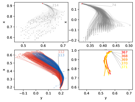
Figure 1: The particle paths for several representative cores. The top two panels show core 214 and core 74 collapsing Alone. Cores 112 and 113 are a binary on the bottom left panel, and can be seen unmixing as collapse proceedes. The bottom right panel shows a cluster of 5 cores, this time showing only the centroids of the cores, which can be seen orbiting each other as they travel and collapse.

3.1 Mode Separation

We begin our analysis by classifying the collapse mode of each core; alone, binary, or cluster. The primary purpose of this is to isolate effects of gravitational collapse from effects of tidal dynamics of neighboring cores during the collapse. Cores that are alone experience only gravitational collapse, so we focus on these in this paper. Binaries also follow these trends. Only about half of cluster cores follow these trends, with the other half dominated by tidal dynamics. It is presently unclear if these cores are similar but we are not able to see it due to limitations of our analysis technique, if these represent a completely different channel for core formation.

For each core, we measure the distance, $\delta$, between its centroid and the centroid of all other cores for all time steps. The number of cores within $\delta=0.05$, $N_{\delta}$, indicates the mode of collapse; alone ($N_{\delta}=1$), binary ($N_{\delta}=2$) or cluster ($N_{\delta}>2$). This simple grading scheme was verified by visual inspection of movies of the collapsing cores. While more sophisticated methods for identifying neighbors can be concocted, this simple scheme is sufficient for our purposes here. Table 1 shows the number of cores in each mode for each simulation. There is a trend that the more strongly magnetized simulations make more alone cores, but detailed conclusions from this unsophisticated method should be taken with a grain of salt.

Figure 1 shows the collapse path in space for several representative cores; two alone, one binary, and one cluster. A track for each particle begins at the dots and end at the red point indicated by the number. The first three panels show every particle for each core, the bottom right panel shows only the centroids of each core in the cluster. The top row shows core 214 and 74, which both form alone. Core 214 forms from a disjoint set, which is spatially a fractal, see Collins et al. (2023) for a more detailed discussion of fractal preimages. Core 74 appears to form from a more continuous region of space, but this is merely a projection effect, it too does not fill the space and has a fractal dimension of 1.6. In the bottom left, cores 112 and 113 begin with their particles mixed, and the gas can be seen to ”unmix” as the collapse proceeds. The bottom right panel shows a cluster of 5 cores, (367, 368, 369, 370, and 371) which all form and evolve near each other. Initially the gas forms in one basin, with the preimage gas mixed together. For clarity, we plot only the centroids of the paths. The orbital dynamics of the cores interacting with one another is clear from the braided paths.

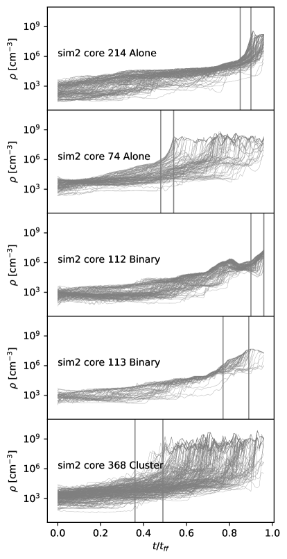
Figure 2: Density vs time for the cores shown in Figure 1. Core 214 collapses much more slowly than 74. The binary pair of 112 and 113 are similar, but not identical. The bottom panel shows the particles for one core that is a member of a cluster. On each panel the first grey line represents while the second grey line represents .

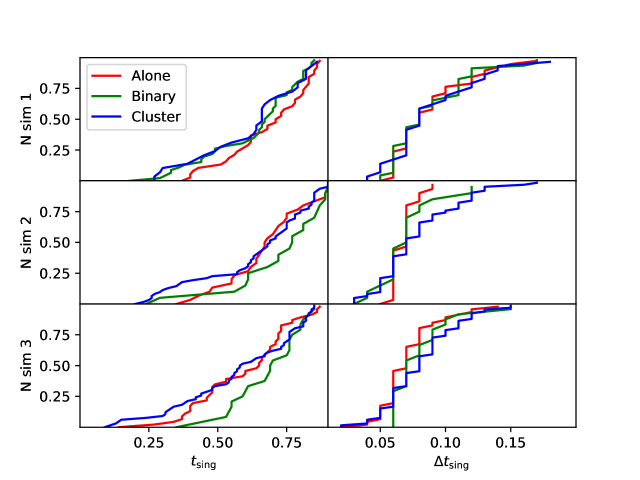
Figure 3: (Left)The cumulative distribution of the singularity time, . For each mode of collapse, the singularity time is nearly uniformly distributed. (Right) The duration of the singularity, which is distributed between $0.05\tff$ and $0.15\tff$.

3.2 Singularity Time: How Fast

Figure 2 shows density vs. time for the cores shown in Figure 1. The purpose of this plot is to indicate the span of timescales and histories demonstrated by cores in these simulations and also to demonstrate the nearly universal cruise-then-collapse behavior. Core 214 is quite slow, not collapsing until near the end of the simulation. Core 74 begins to get dense much earlier, with a few particles reaching high density early, and the remaining particles accreting over the remainder of the simulation. Note that the majority of the mass is delivered by , see Section 3.4.3, the remaining particle accretion does not tend to represent a large mass flux.

The third and forth panels of Figure 2 show the binary pair of 112 and 113. The pair shows similar density behavior until they separate at $\sim 0.75\tff$. In fact, core 113 collapses first, with 112 still increasing in density at the end of the simulation.

Core 368 is a member of a cluster with 5 other cores, and the final panel of Figure 2 shows the particles of only that core. This core also collapses fast, but has a much more protracted and chaotic assembly history after the initial collapse. We will revisit the more complex dynamics of cluster formation in Section 3.6.

The vertical lines in each curve in Figure 2 indicates the onset of collapse (, first line) and the end of collapse (, second line). is defined as the point at which the gas begins to get very dense. By various theorems one learns in calculus, before the density gets large, the time derivative of density must becomes large. It was found empirically that the collapse is preceded immediately by $\dbd{\rho_{\rm{max}}}{t}>10^{5}$ in code units, where $\rho_{\rm{max}}$ is the max density of the preimage gas. Thus $\tsing$ is defined as the time at which the derivative of the peak density is first larger than $10^{5}$. We further define  as when $\dbd{\rho_{\rm{max}}}{t}=0$ for the first time after , that is when the peak density is reached. For these simulations,  and  thus described show us an excellent view of how and when the cores collapse.

The cumulative distribution of  can be seen in the left column of Figure 3. Each row shows a different simulation. Red lines show alone cores, green shows binaries, and blue shows clusters. For each population, the cumulative distribution indicates that the distribution of  is relatively uniform between $0.25\tff$ and $1\tff$ when the simulation ends. Some fluctuations exist, but no consistent trends are noticeable.

The right column of Figure 3 shows the distribution of the duration of the initial singularity, $\Delta t_{\rm{sing}}=\tsung-\tsing$. Note that the axes between the left and right columns are not the same, this is a tight distribution around $0.1\tff$. The collapse shows a nearly universal short duration.

3.3 What sets ?

It would be extremely useful to understand what made some cores collapse faster than others. Unfortunately, after examining many possible correlations, we find that the only thing that is reliably correlated with  is the number of particles in the core. For each simulation, we examine Pearson $R$ for each core relative to several mass-weighted average quantities. Pearson $R$ measures the degree of linear correlation between two quantities, with -1 being perfectly anti-correlated. We find that, for a number of quantities, the degree of correlation is -0.35 or less, with the exception of the number of particles, which is mildly anti-correlated with R=-0.5. It is difficult to draw a causal relationship from such weak correlations.

Table 2 shows Pearson $R$ for $\tsing$ and a number of quantities. These include the number of particles, $N_{\rm{particles}}$, the volume of the convex hull bounding the particles, $V_{\rm{hull}}$, the mean density, $\overline{\rho}$, the mean gravitational binding energy, $\overline{E_{G}}$, the mean kinetic energy, $\overline{E_{K}}$, the velocity dispersion, $\sigma_{\rm{3d}}=\sqrt{\overline{\vvec^{2}}}$, the mean radial velocity, $\overline{v_{r}}$, the mean tangential velocity $\overline{v_{t}}$, and the free-fall-time of the core, $\tff=\sqrt{3\pi/32G\overline{\rho}}$. While the trends are in the direction one would expect (e.g.  is positively correlated with  as computed for that preimage) the scatter is too large to be predictive.

Table 2: Pearson R between properties, Q, for each core and their singularity time, $\tsing$. No substantial correlations are seen.

Q
$N_{\rm{particles}}$	-0.49	-0.55	-0.45
$V_{\rm{hull}}$	-0.27	-0.04	-0.14
$\overline{\rho}$	-0.27	-0.42	-0.42
$\overline{E_{G}}$	-0.13	-0.26	-0.42
$\overline{E_{K}}$	-0.28	-0.29	-0.33
$\sigma_{3d}$	-0.16	-0.01	-0.07
$\overline{v_{r}}$	-0.13	-0.02	-0.07
$\overline{v_{t}}$	-0.17	-0.02	-0.07
$t_{\rm{ff}}$	0.13	0.37	0.19

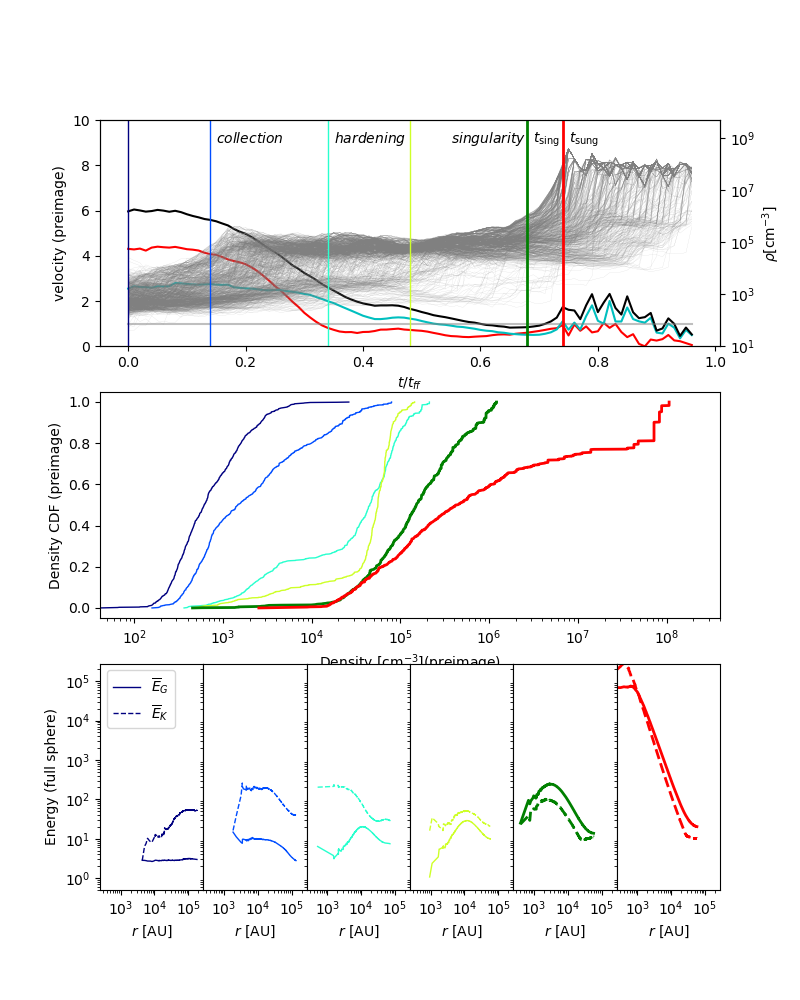
Figure 4: The collapse of one core and its phases. (top row) Density (grey lines, right axis) and velocity (red, teal, and black lines, left axis). Vertical lines denote the times of analysis for the second and third rows. These are the beginning (navy) the middle of the hardening phase (light blue), the end of the hardening phase (light green), the beginning of singularity (dark green) and the “end” of singularity (red). (middle row) Cumulative density distribution at the 5 indicated snapshots. (bottom row) Radial profiles of of $\overline{E}_{G}$ vs $\overline{E}_{K}$ for each of the 5 snapshots.

3.4 Collapse Paradigm

To further understand the processes at work, we would like to examine $\rho_{i}(t)$ for every particle, $i$, in every core, as well as velocity, kinetic, and gravitational energies. This is several thousand plots. We summarize these plots by way of a case study (this section), followed by an ensemble of cores (next section). The interested reader can see the next few figures for each of our cores at our website, cores.dccollins.org.

3.4.1 4 stages

We find that each core goes through four stages of collapse to one degree or another. We refer to these as collection, hardening, singularity, and mosh. Not every core experiences each stage, the only two that are present for every core are hardening and singularity. The collection stage sweeps low density gas together by converging supersonic flows; kinetic energy is typically larger than gravitational, but not universally. During the hardening stage, the density becomes moderately high ($\sim 10\rho_{0}$), the velocity decays to trans- to slightly super-sonic, and gravitational and kinetic energies equilibrate. During the singularity, density rises extremely fast and the majority of the mass is delivered to the core in $\sim 0.1\tff$; gravitational energy dominates. By the end of the singularity, the core is a $r^{-2}$, but not generally spherical, and the ratio of kinetic to gravitational energy follows a remarkably consistent pattern dropping from $E_{K}/E_{G}\sim 4$ at the inner radius and $E_{K}/E_{G}=0.5-2$ at outer radii. After the singularity is the last stage, the mosh, wherein tidal dynamics from neighboring cores and rotational dynamics of the core itself can break cores into fragments, merge cores together, and cause erratic trajectories. We demonstrate the first three stages in Figure 4. Owing to the more widely varied chaos of the tidal dynamics in small multiples, we primarily focus on isolated objects in this work. We briefly describe the fourth stage in Section 3.6.

3.4.2 Case Study

In Figure 4 we show the collapse history of one representative core (core 114 from $sim2$) outlining three of the four stages of collapse. This core collapses alone, so it does not experience the mosh stage. This plot summarizes how density, velocity, gravitational energy, and kinetic energy change in concert with one another. The top row shows the preimage density, one line for each particle (grey lines, right axis) and the average velocity (r.m.s in black, radial velocity in red, and tangential velocity in teal, left axis). Also indicated are six snapshots in time (vertical bars). The second row shows the cumulative density distribution for preimage density at each of those snapshots. The third row shows radially averaged kinetic and gravitational energy for a sphere surrounding the particles at each snapshot. The first two rows utilize only the preimage gas, while the third row measures $E_{G}$ and $E_{K}$ on spheres centered on the centroid of the particles. While this figure is somewhat elaborate, it is useful to see how each of these quantities changes in concert with one another. We will elaborate on each of these in turn.

Six snapshots in time, indicated by the vertical bars in the top row of Figure 4, highlight the stages of the collapse; the initial conditions (navy), the collection stage (light blue), the hardening stage (teal and light green), the beginning of singularity (, dark green), and the end of singularity (, red). This core does not experience the mosh stage. We do not presently have a quantitative boundary between collection and hardening, as no consistent trends are obvious (see Section 3.5).

The top row in Figure 4 also shows the density and velocity behavior of this core. Density begins low, sampling the turbulent density field, as discussed in Collins et al. (2023). The total velocity is initially quite large, $v_{rms}=6c_{s}$ in this core (not universal). During the collection stage (blue lines), the large scale flow collects the material into a smaller, higher density patch. During the hardening stage (teal, light green lines), the density distribution becomes more narrow and the velocity decays. For this core, the radial velocity becomes transsonic by $t=0.3\tff$, at which time a disk begins to form and the tangential velocity increases over the radial. The r.m.s velocity is subsonic at the start of singularity, but this is also not a universal feature among all cores. After the end of the singularity, the core accrets the remaining particles. As we discuss in Section 3.4.3, this stage does not accrete much mass, the vast majority of the mass is assembled during the singularity.

The second row in Figure 4 shows the cumulative preimage density distribution at each of the six snapshots. At the first time (navy line), the density is roughly lognormal, as it samples the turbulent initial conditions. This core begins in a large converging flow which sweeps most (80%) of the particles to moderate density ($\rho=10-100\rho_{0}$), while some remains lower ($\rho=10\rho_{0}$). During the hardening stage, the moderate-density gas gets moderately more dense, and the low density gas is compressed, but the peak density does not increase dramatically. During the singularity (between the dark green and red lines), the peak density increases rapidly. Roughly 20% of the particles are above a density of $10^{7}\percc$ at the end of the collapse.

The third row in Figure 4 shows the gravitational and kinetic energies of the gas on spheres surrounding the particles. The dotted line shows kinetic energy, averaged over the sphere of volume $V(r)$, and the solid line shows the magnitude of gravitational energy:

$$\overline{E}_{G}(r) =\frac{1}{V(r)}\int_{0}^{r}\frac{\left(\nabla\phi\right)^{2}}{8\pi G}d^{3}x$$ (1)

$$\overline{E}_{K}(r) =\frac{1}{V(r)}\int_{0}^{r}\half\rho(v-\bar{v})^{2}d^{3}x$$

where $V(r)$ is the volume of a sphere with radius $r$. Initially the gravitationally energy is flat and kinetic is several times larger. By the end of the hardening stage (light green line) the profiles of $E_{G}$ and $E_{K}$ have been driven toward each other. Singularity drives an enormous increase in both kinetic and gravitational energies, and we’re left with a virialized sphere with a rapidly rotating object in the center.

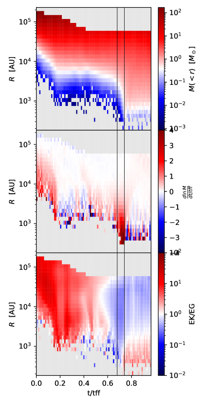
Figure 5: Extremely rapid assembly of mass. All three plots show azimuthally averaged quantities on a sphere centered on the particles, but taking all zones. The left vertical axis is radius in AU, the horizontal axis is time in units of the free fall time. Vertical black lines show  and . (Top) Interior mass, $M_{<}$ The mass is assembled to the center extremely rapidly between  and , with relatively little accretion after . (Center) The relative mass accretion rate. Very little accretion happens after . (Bottom) The ratio of kinetic and gravitational energies. Immediately after , the energies show that the core forms a virialized object with a rapidly spinning disk in the center. During the singularity, gravitational energy dominates.

3.4.3 Mass Delivery

We now examine the nature of the gas mass during the collapse. Figure 4 only shows density of the preimage gas, which covers a sparse subset of the surrounding material, and by the end it gives only location information. It is valuable to also make a complete census of the gas around the collapsing object.

Figure 5 shows mass vs. time and radius At each time, a sphere of gas is extracted that is centered on the centroid of the particles and has a radius equal to the most distant particle. The particles all collapse to a few zones at the end, so the analysis sphere has a minimum radius of one root-grid-zone. The vertical lines show  and .

The top panel shows interior mass vs time,

$$M(<r) =\int_{0}^{r}\rho d^{3}x$$ (3)

$$:=M_{<}$$

The colorbar is arranged so that the white line follows a mass $M_{1000}$, which is the mass interior to $1000\rm{AU}$ at the end of the simulation. It should be noted that this is not, strictly speaking, a Lagrangian surface, since there is substantial flux both in and out of this surface. It does show that the mass is assembled at the center of the core rapidly during the singularity, and then remains relatively constant.

The middle panel shows the normalized relative accretion rate:

$$q =\ddbd{\ln M_{<}}{t/\tff}$$

This is computed by way of finite differences of the binned $M_{<}$ in the top plot. We see a large positive accretion rate during the collection phase ($t<0.2\tff$), followed by a high degree of volatility, fluctuating around zero. Beginning at  and ending at , $q$ grows to a factor of several as most of a solar mass is delivered to the center in 0.1 . Then the high frequency rotational motions of the disk make the mass fluctuate in its location, but not gain much overall mass. The lack of growth in mass is due to the fact that the object is virialized, with large kinetic energy.

The third panel of Figure 5 shows the ratio of kinetic to gravitational energy, $E_{K}(r)/E_{G}(r)$, both defined in Equation 1. A value of 2 is the often quoted value for virialization. The colorbar is tuned so that $E_{K}(r)/E_{G}(r)=1$ is white; gravitationally dominated gas is in blue, and kinetic energy dominated gas is in red. It is seen that at the beginning of the simulation, kinetic energy dominates the bulk of the flow. As time progresses during the hardening phase, the ratio grows to roughly unity. During the singularity, gravity dominates the entire sphere, and immediately after  we find a pattern slightly dominated ($E_{K}/E_{G}=2$) by kinetic energy, and transitions to $E_{K}(r)/E_{G}(r)=0.5$ in the outer regions. This is a relaxed object, as much as is possible. The canonical value of virialization, $E_{K}/E_{G}=2$, is for an object for which is in vacuum and has the second derivative of its moment of inertial identically zero. We see values that are of order 2, stationary in time, and have profiles that are consistent from core to core.

It should be noted that these dynamics are visible to us because we did not use sink particles. Sink particles (Teyssier & Commerçon, 2019) are a useful tool to follow self-gravitating simulations in time, but they are a subgrid model selected by the simulator, and the accretion rate they give is, while generally reasonably constructed, dramatically influenced by the parameters of the sink. Here we allow the dynamics to unfold self-consistently, at the cost of shortened simulation time. This allows us to measure how singular collapse from turbulent initial conditions unfolds.

Violent relaxation (Lynden-Bell, 1967) is a mechanism by which an ensemble of stars can relax to a stable configuration in a free-fall time. This is typically studied in a collisionless system, which has the nice property that phase space volume is conserved. The hallmark of violent relaxation is the dramatic change of the potential in time, which serves to equilibrate the system quite quickly. Here we see a similar process. Violent relaxation has also been studied in star forming clouds by Bonilla-Barroso et al. (2022), where they examine the process on the clump (few pc) scale. This is similar, but happening on an individual star (0.1 pc) scale.

3.5 Ensemble properties

The previous section examined one core in detail. Now we examine a larger sample of cores to see how many of these traits are universal, and how many have some variation. We restrict our examination here to cores that form alone, from the first simulation . Binary cores, and cores from the other simulations, follow indistinguishable trends. A fraction of cluster cores do as well but many cluster cores have much more complex velocity signatures and are likely not actually relaxed at the end of the simulation. We revisit binaries and clusters cores in Section 3.6. There is no obvious distinction between the simulations for any of the plots in this section, so we restrict ourselves to one simulation.

3.5.1 Mean density and velocity of preimage gas

Figure 6 shows mean quantities on preimage gas for every core in the sample. Each core has been scaled in time to its own . The top row shows mean density, $\overline{\rho}$, which shows a universal behavior of slow increase followed by a transition to a free-fall solution (cruise-then-collapse). The second row shows the r.m.s. velocity of the preimage gas, $\overline{v_{\rm{rms}}}$. The flow begins highly supersonic in total. Velocity decays by  to a Mach number of a few. The third row shows the mean radial velocity, $\overline{|v_{\rm{radial}}|}$. Interestingly, there is not a universal trend of large converging flow, in fact some cores have very small radial velocities initially. To the extent that the collection stage is real, this can be seen in this plot as large radial velocities that decay to transsonic to slightly supersonic. Finally, note that this is the absolute value of the radial velocity, but all mean velocities are negative. By , the radial velocity is clustered around transsonic. Some are subsonic, as expected by others, while some are slightly supersonic. The fourth row shows the tangential velocity, which is universally supersonic initially, and decays to transsonic before .

Post , the very high frequency and high velocity of rotating disks can be seen. In this stage, the particles occupy only a few zones at the center of each object, and are subject to the high frequency chaotic dynamics. Many of these form clearly defined disks.

3.5.2 Mass Delivery

The fast mass delivery for each core can be seen in Figure 7. Here we define $R_{1000}$ as the radius that contains a mass of $M_{1000}$, which is defined as the mass within 1000 AU at the end of the simulation. The edge of a core is poorly defined, so to avoid murky clump definitions we adopt a fiducial radius. This can be seen as the white line in the top panel of Figure 5 for one core. In Figure 7, we show $R_{1000}$ for each core vs. time, scaled to the cores own . Most cores deliver the bulk of the mass of the final object beginning at and taking about 0.1  to get there. A few behave slightly differently, as these are ultimately chaotic dynamics. Note that this plot measures all gas, not just preimage gas.

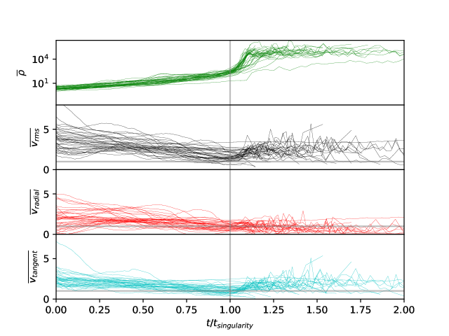
Figure 6: Tracks for all of the alone cores from , each one scaled to its respective . Each line represents a core. (Row 1) Mean density of preimage gas. A consistent profile can be seen of slow increased followed by free-fall. (Row 2) RMS velocity of preimage (particle) gas. The total velocity remains quite large. (Row 3) Radial velocity of the primage. Radial velocity has not prefered initial configuration, some begin with large convergence, some not. By , the radial velocity is clustered around transsonic. (Row 4) Tangential velocity of the primage. Universally supersonic at the beginning, beoming transsonic by .

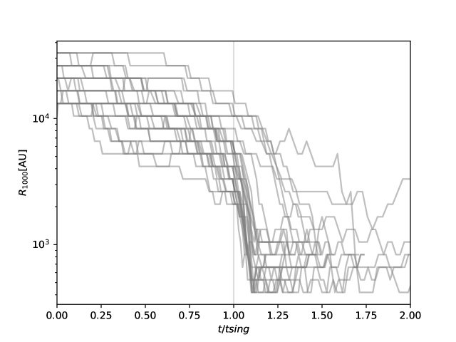
Figure 7: $R_{1000}$ is the radius containing a mass of $M_{1000}$, which is defined as the total mass within 1000 AU at the end of the simulation. All cores deliver the bulk of their mass to the center within 0.1  of .

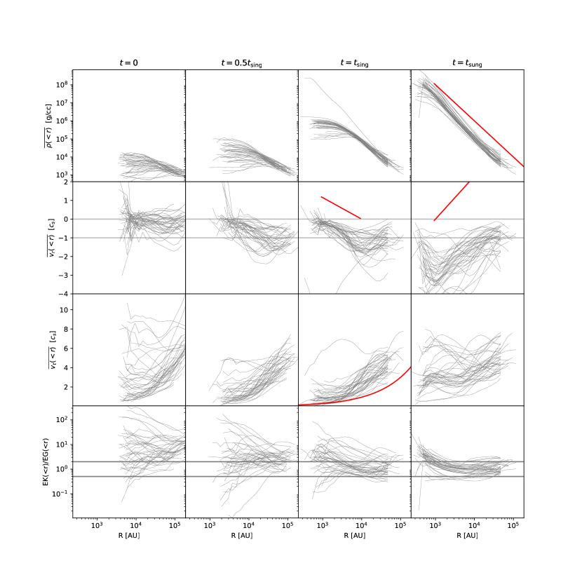
Figure 8: Radial profiles $\bar{Q}(r)$ for several quantites (rows) at several frames (columns) for every alone core (grey lines). Four times at t=0, $t=0.5\tsing$, , and are shown. Note that  and are different for each core. The rows show mean density, radial velocity, tangential velocity, and ratio of gravitational to kinetic energy. Notable features are highlighted by red lines, see text for details.

3.5.3 Radial Profiles at  and

Figure 8 shows azimuthally averaged quantities for spheres around every core (grey lines) at four different times (columns). The four columns show $t=0$, $0.5\tsing$, $\tsing$, and $\tsung$. Note that $\tsing$ and $\tsung$ are different for every core, see Section 3.2 for definitions and distributions. The rows show azimuthal averages vs. radius for several quantities. We make the radial interior average, , for several quantities as

$$\qbar=\frac{1}{V(r)}\int_{V(r)}Q(\xvec)d^{3}\xvec$$ (4)

where $V(r)$ is a sphere centered on the centroid of particles. Here we examine density, $\overline{\rho}$, radial velocity $\overline{v_{r}}$, tangential velocity $\overline{v_{t}}$, and the ratio of gravitational to kinetic energy, $\overline{E_{K}}/\overline{E_{G}}$.

The first row shows average interior density,

$$\overline{\rho}(r)=\frac{1}{V(r)}\int_{V(r)}\rho(\xvec)d^{3}\xvec$$ (5)

for every core at four frames. This is the average density within a radius $r$. At $t=0$, density is roughly flat. As discussed in Collins et al. (2023), this is a result of the density correlation length being significantly shorter than the size of the preimage gas. By $0.5\tsing$, a centrally condensed object is beginning to form, some of them have developed an outer region that follows a $\rho\sim r^{-2}$ behavior. By , the central densities have grown somewhat and all objects begin to resemble Bonner-Ebert spheres (Ebert, 1955; Bonnor, 1956). In the small window between  and , the central density increases by many orders of magnitude, and the objects are all universally singular isothermal spheres.

The second row of Figure 8 shows mean interior radial velocity,

$$\overline{v_{r}}(r)=\frac{1}{V(r)}\int_{V(r)}(\vvec(\xvec)-\vvec_{c})\cdot(\hat{r}_{c})d^{3}\xvec$$ (6)

This is the average radial motion within a radius $r$, relative to the central velocity for the core, $\vvec_{c}$, along the radial unit vector for that core, $\hat{r}_{c}$. At $t=0$, the radial velocity does not have a ”typical” trend, some contracting and some weakly expanding. By the end of the collection phase at $0.5\tsing$, the radial velocity is negative for all particles. Note that at early phases, the curve of $\overline{v_{r}}(r)$does not, in general, go to zero as $r\rightarrow 0$. This is due to the fractal and chaotic nature of the preimage gas; the geometric center, the center of mass, and the center of velocity are not at the same point in space. By , the object is not a fractal mess (well, less of a mess) and the radial velocity tends to be logarithmic in radius, and subsonic. We posit that this phase is what is observed as a coherent core. Between  and , the majority of the mass is delivered to the center by negative radial velocity. After the relaxation event, at , the radial velocity behavior is now increasing with radius, and generally supersonic:

$$\overline{v_{r}}(r)\propto\begin{cases}\ln\left(\frac{r}{r_{0}}\right)^{-1/2}&t=\tsing\\ \ln\left(\frac{r}{r_{0}}\right)^{+1}&t=\tsung.\end{cases}$$ (7)

This reversal happens by way of a wave that travels inwards. The wave follows the knee in the density profile.

The third row of Figure 8 shows tangential velocity,

$$\overline{v_{t}}(r)=\frac{1}{V(r)}\int_{V(r)}||((\vvec-\vvec_{c})-\vvec_{r})||d^{3}\xvec$$ (8)

which is just the full velocity less the radial in the frame of the core. Also plotted in the third panel is a typical turbulent velocity expected from theory, $v_{\rm{turb}}=3\sqrt{r/r_{0}}$ for $r_{0}=0.1$. Core profiles are bounded below by this turbulent velocity. During the hardening, the tangential velocity maintains roughly a profile like $\sqrt{r}$, decreasing in magnitude. After the singularity, disks form in the central region and the tangential velocity becomes quite large and no longer centered on zero velocity.

In the fourth row of Figure 8 we show the ratio of kinetic to gravitational energy. We define gravitational energy $E_{G}$ and kinetic energy $E_{K}$ as in Equation 1 and we plot their ratio. In the first panel, at $t=0$, we find that the ratio tends to decrease with radius (though not universally). This can be understood again as a signature of the turbulent initial conditions. The kinetic energy, $E_{K}$, increases as roughly $r$, since the total velocity is subject to turbulent statistics, and $v(r)\propto\sqrt{r}$. On the other hand, we integrate over several density correlation lengths, so that average density is roughly constant and tends to the mean density. Thus their ratio is roughly linear in radius. This is a little counter intuitive, and can be understood because one preimage region covers many density fluctuations, so there is on average no net acceleration vector. During the hardening phase, $E_{G}$ and $E_{K}$ both increase until they are more-or-less equal. Large values of $E_{K}/E_{G}$ are seen at the center, while the ratio adjusts to be between 0.5 and 2 by 10,000 AU. During the singularity between  and , the material at the center accelerates into a disk, and the ratio aligns to be roughly 2 at the center, between 0.5 and 2 for larger radii. A value of $E_{K}/E_{G}=2$ is expected for idealized virialized systems. The $E_{K}/E_{G}$ profile for objects at the end of the singularity is extremely consistent. The velocity profiles fluctuate a substantial amount from core-to-core, but the density profile and energy ratio profile are extremely consistent.

3.6 Multiples and Mosh

Until now, we have focused on alone cores. When stretched to their singularity time, a clear behavior of velocity decay followed by violent relaxation is seen. Binaries and clusters exhibit similar properties, with a few exceptions. It should be noted that the ultimate fate of binaries and clusters is not known to us, as we only simulate a short duration in time.

Binaries in our simulation are observed to form in one of two ways. Either one singularity forms, which then breaks into two as the large orbital kinetic energy it gained by falling down the potential well breaks the object in two; or two singularities form in the same basin, which then begin to orbit one another. In both cases, the behavior is similar to that described in Section 3.4. A future study will explore more details.

Clusters similarly form multiple singularities, some of which fragment, and some of which merge, and some of which cause substantial tidal torques on other cores. Many of these do not show the same transition to coherence that is seen in alone or binary cores. We examine one particularly large cluster core in detail to demonstrate the differences that exist.

Figure 9 shows the fourth phase, mosh, using core 9 from . This core is a member of a cluster with several other cores, none of which are shown. In these three figures, every particle is plotted with a grey line that has an opacity of 0.1, meaning that as they overlap in space the lines get darker. As particles collapse, many particles are compressed into the same zone (Collins et al., 2023), which makes the lines darker proportional to the number of particles in the zone, and proportional to the density in the zone. In the top plot, we see the entire collapse from $t=0$ (grey points) to the end (red point at y=0.1 z=0.05). The second panel shows a zoom-in of the pink region denoted in the top panel. This shows sub clumps forming, orbiting each other, merging, and getting ejected by a close encounter with other cores.

The bottom panel of Figure 9 shows density (right axis) and velocity (left axis) as in Figure 4. The mean radial and tangential velocities are quite large until the core is ejected from the cluster at $t=0.8\tff$, after which the velocity dispersion is zero due to the fact that all the particles occupy a single zone. The r.m.s. velocity is always extremely large because of the orbital dynamics of sub clumps, which in this analysis framework are all treated as one. It is possible that the sub clumps do transition to coherence and we are unable to see it; it is possible that they don’t, and there are multiple channels for star formation. We will address this in a future work.

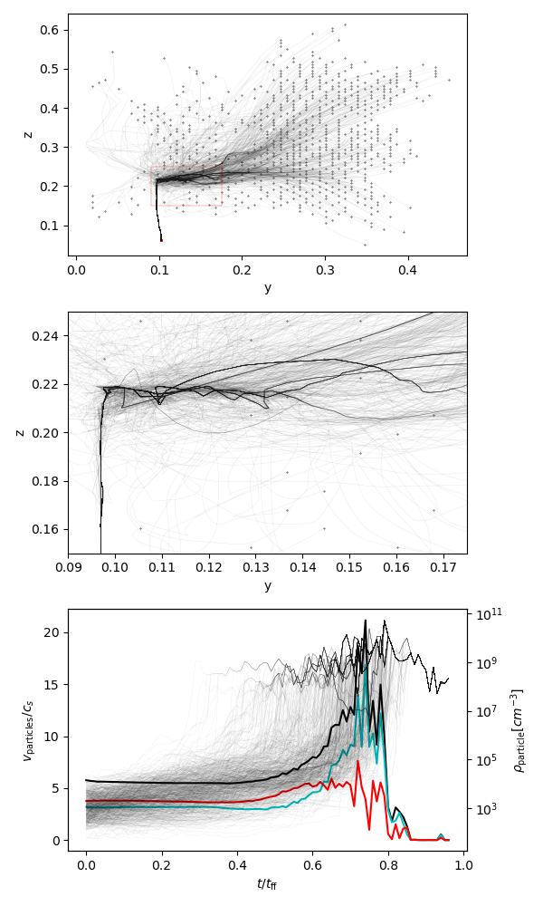
Figure 9: (Top) Path lines for all particles for cluster core 9 from . Particles begin at the dots and end on the red point at the bottom. Multiple centers of collapse can be seen, which aggregate until a close encounter ejects the newly formed core from the cluster. (Middle) a close up of the late stage tidal dynamics. (Bottom) As in Figure 4, particle density (right axis) and velocity (left axis), with (total, tangential, radial) velocity in (black, teal, red). The tidal dynamics before the ejection dominate the velocity signal. Mean velocities go to zero as the particles are all driven into a single zone.

4 Conclusions

In this work, we examine how the high vacuum of outer space becomes stars. We did this by embedding a fleet of pseudo-Lagrangian tracer particles in a turbulent, collapsing molecular cloud; identifying dense cores and the particles within; and then examining the density, velocity, and energetics of each particle. One important aspect of this study is our lack of sink particles, which allows us to examine the collapse without the use of subgrid models that directly influence the collapse. This decision limits the duration of the study in exchange for self-consistency of the collapse.

We find that collapse happens in four stages; collection, hardening, singularity, and mosh. The specifics are unique to each core, and many cores do not experience collection or mosh stages. During collection, low density, high velocity gas is swept into moderate density object by converging flows. Sometimes these are initially dominated by gravity, sometimes by kinetic energy. During the hardening phase, gravitational and kinetic energy both increase to rough equipartition. During the singularity, the density gets very high, mass is delivered to the center of the object, and a relaxed object is formed. This is a universally fast event, lasting $\sim 0.1\tff$. At the end of singularity, a relaxed object remains, with kinetic-to-gravitational energy ratio that varies logarithmically from about 2 at the center to about 0.5-2 at 10,000 AU. We demonstrate this in detail for one representative object in Section 3.4, and the variation in mean quantities in Section 3.5.

This can be seen as two transitions to coherence; one in which velocity of the gas that will collapse becomes low, and one in which the kinetic and gravitational energies virialize. The first is analogous to those subsonic or trans-sonic cores (Pineda et al., 2010; Singh et al., 2021; Choudhury et al., 2021). The second is the fast virialization of the object, akin to violent relaxation, wherein the potential undergoes rapid evolution towards a virialized object. Most studies of violent relaxation are done in collisionless systems, here we have supersonic flow which does not preserve phase space to the same extent.

We find that roughly half of all binaries form from two points of singularity that then begin to orbit one another, while the other half form from one singularity that fragments into two distinct objects. Our definition of a binary system is unsophisticated, so we refrain from detailed statistical analysis.

We find that most higher order multiple systems have different velocity signatures when analyzed through this lens, owing to the chaos of the tidal dynamics of substructure during the collapse. The present analysis cannot determine if this transition to coherence happens multiple times, or if something entirely different is happening.

Our study shows similarities with other recent works. The three phase view of Offner et al. (2022) used machine learning techniques on similar simulations to organize the flow. They find that core experience three phases, turbulence, coherence, and collapse, which are similar in spirit to our collection, hardening, and singularity. Similarly the inertial flow model Pelkonen et al. (2021) has high velocity streamers delivering the bulk of the mass to the core, which can be seen during the singularity stage in our work. These works are quite similar in setup and simulation software to our own, differences in conclusions are due mostly to differences in the lenses we use to view our simulations. The physics of self-gravitating turbulence is central to astrophysics, but underpinned by chaos, so many views are necessary to unpack the true dynamics.

Data Availability

Simulation data present here is available on request (dccollins@fsu.edu).

References

- Alves et al. (2007) Alves J., Lombardi M., Lada C. J., 2007, A&A, 462, L17
- Balsara (2001) Balsara D. S., 2001, \jcompphys, 174, 614
- Berger & Colella (1989) Berger M. J., Colella P., 1989, \jcompphys, 82, 64
- Bonilla-Barroso et al. (2022) Bonilla-Barroso A., et al., 2022, MNRAS, 511, 4801
- Bonnor (1956) Bonnor W. B., 1956, MNRAS, 116, 351
- Bryan et al. (2014) Bryan G. L., et al., 2014, ApJS, 211, 19
- Chabrier (2003) Chabrier G., 2003, PASP, 115, 763
- Choudhury et al. (2021) Choudhury S., et al., 2021, A&A, 648, A114
- Collins et al. (2010) Collins D. C., Xu H., Norman M. L., Li H., Li S., 2010, ApJS, 186, 308
- Collins et al. (2011) Collins D. C., Padoan P., Norman M. L., Xu H., 2011, ApJ, 731, 59
- Collins et al. (2012) Collins D. C., Kritsuk A. G., Padoan P., Li H., Xu H., Ustyugov S. D., Norman M. L., 2012, ApJ, 750, 13
- Collins et al. (2023) Collins D. C., Le D., Jimenez Vela L. L., 2023, MNRAS, 520, 4194
- Crutcher (2012) Crutcher R. M., 2012, ARA&A, 50, 29
- Crutcher et al. (2009) Crutcher R. M., Hakobian N., Troland T. H., 2009, ApJ, 692, 844
- Ebert (1955) Ebert R., 1955, Z. Astrophys., 37, 217
- Federrath et al. (2008) Federrath C., Glover S. C. O., Klessen R. S., Schmidt W., 2008, Physica Scripta Volume T, 132, 014025
- Gardiner & Stone (2005) Gardiner T. A., Stone J. M., 2005, \jcompphys, 205, 509
- Goodman et al. (1998) Goodman A. A., Barranco J. A., Wilner D. J., Heyer M. H., 1998, ApJ, 504, 223
- Hennebelle & Chabrier (2011) Hennebelle P., Chabrier G., 2011, ApJ, 743, L29
- Krumholz & McKee (2005) Krumholz M. R., McKee C. F., 2005, ApJ, 630, 250
- Ladjelate et al. (2020) Ladjelate B., et al., 2020, A&A, 638, A74
- Li et al. (2008) Li S., Li H., Cen R., 2008, ApJS, 174, 1
- Lynden-Bell (1967) Lynden-Bell D., 1967, MNRAS, 136, 101
- Mac Low (1999) Mac Low M.-M., 1999, ApJ, 524, 169
- Mignone (2007) Mignone A., 2007, \jcompphys, 225, 1427
- Miville-Deschênes et al. (2017) Miville-Deschênes M.-A., Murray N., Lee E. J., 2017, ApJ, 834, 57
- Mouschovias (1987) Mouschovias T. C., 1987, in Morfill G. E., Scholer M., eds, NATO ASIC Proc. 210: Physical Processes in Interstellar Clouds. pp 491–552
- Offner et al. (2022) Offner S. S. R., et al., 2022, MNRAS, 517, 885
- Padoan (1995) Padoan P., 1995, MNRAS, 277, 377
- Padoan & Nordlund (2011) Padoan P., Nordlund Å., 2011, ApJ, 730, 40
- Pelkonen et al. (2021) Pelkonen V. M., Padoan P., Haugbølle T., Nordlund Å., 2021, MNRAS, 504, 1219
- Pineda et al. (2010) Pineda J. E., Goodman A. A., Arce H. G., Caselli P., Foster J. B., Myers P. C., Rosolowsky E. W., 2010, ApJ, 712, L116
- Rosolowsky et al. (2008) Rosolowsky E. W., Pineda J. E., Kauffmann J., Goodman A. A., 2008, ApJ, 679, 1338
- Shu et al. (1987) Shu F. H., Adams F. C., Lizano S., 1987, ARA&A, 25, 23
- Singh et al. (2021) Singh A., et al., 2021, ApJ, 922, 87
- Skillman et al. (2013) Skillman S. W., Xu H., Hallman E. J., O’Shea B. W., Burns J. O., Li H., Collins D. C., Norman M. L., 2013, ApJ, 765, 21
- Solomon et al. (1987) Solomon P. M., Rivolo A. R., Barrett J., Yahil A., 1987, ApJ, 319, 730
- Teyssier & Commerçon (2019) Teyssier R., Commerçon B., 2019, Frontiers in Astronomy and Space Sciences, 6, 51
- Towns et al. (2014) Towns J., et al., 2014, Computing in Science and Engineering, 16, 62
- Turk et al. (2011) Turk M. J., Smith B. D., Oishi J. S., Skory S., Skillman S. W., Abel T., Norman M. L., 2011, ApJS, 192, 9
- Xu et al. (2012) Xu H., et al., 2012, ApJ, 759, 40