Abstract

We consider a non-minimally coupled Einstein-Maxwell gravity with no $U(1)$ symmetry property to study stability of an electrostatic star via canonical quantization approach and obtain that the stability is free of gauge field effects. By calculating the Hamiltonian density of the stellar system we show that the corresponding Wheeler-DeWitt wave functional is similar to a simple harmonic quantum Oscillator for which a non zero ADM mass of the system causes a quantization condition on the metric fields. Probability wave packets are described by the Hermit polynomials. Our mathematical calculations show that in this approach of quantum gravity the metric fields are regular for all values of the electric potential and so the quantized spacetime has not both of event and apparent horizons. The most probability of the quantized line element is for ground state of the system. To check validation of the model we use Bohr‘s correspondence principal and generate directly semi classical approach of the quantized metric states at large quantum numbers where they reach to Schwarzschild like metric according to the Birkhoff’s theorem. Also we check that the generated semi classical solutions are satisfied exact classical metric solutions which are obtained from Euler Lagrange equations. We show that ‘charge to mass ratio‘ of the electrostatic star is a constant defined by the coupling constant of the model and it is in accord to other alternative approaches.

1 Introduction

The famous singularity theorems show that the classical theory of general relativity is incomplete, because these are causal and so under general conditions are unavoidable (see Chapter 9 in ref [1]). In fact these singularities reach to some infinite values for energy density and so curvature of curved spacetimes in a gravitational system under consideration. Conceptually, physicists hope the singularity problems resolved via generalization of the quantum field theory to gravity or equivalently to curved spacetimes. This idea comes from history of the classical mechanics which happened at first of twentieth century by extending it to the quantum mechanics and quantum field theory in flat Minkowski spacetime respectively for nonrelativistic and relativistic particles. In fact, this is the main reason why we are looking for full quantum gravity. In general, to construct full quantum theory of gravity, there are several approaches which are formulated and basically are different from each others. In short they are as follows [2]: (a) Quantum general relativity which is application of ‘Dirac‘s quantization rules‘ to classical general relativity. These approaches are done with two different methods called as ‘covariant approaches‘ which means utilizes of four-dimensional covariance for studying of the system under consideration, such that perturbation theory [3], [4] or path integral methods [5] and ‘canonical approaches‘ where one makes a Hamiltonian formalism and produces some appropriate canonical variables with corresponding conjugate momenta. Some examples to the latter formalism are quantum geometrodynamics [6] (see also [7] for applications in quantum cosmology with supersymmetric perspective) and loop quantum gravity [8]. (b) String/M-theory which is main approach to construct a unifying quantum framework of all interactions of gravitational and matter fields (see for instance [9] and [10]). (c) Quantum gravity from topological quantum field theory approaches (see for instance [11] and [12]).
Interaction of quantum matter fields with black holes which produces the well known Hawking radiation [13], [14] which means evaporation of the black holes, predicts that the full quantum gravity is dominated at scales below the Planck scales $\ell_{p}\approx 1.62\times 10^{-33}cm$ (see for instance Page 2 of ref. [2]) and for scales larger than of $\ell_{p}$ the geometry/gravity behaves classically but not other matter fields. In the latter case the matter fields behave as quantum fields which renormalized expectation values of whose stress tensor operator are used as right side of the Einstein‘s metric equation $G_{\mu\nu}=-8\pi G<\hat{T}_{\mu\nu}>_{ren}.$ This equation is called backreaction equation of the matter quantum fields effecting on the classical metric field and its solutions give us modified background classical metric (see Chapter 14 in [1]). This approach of quantum gravity is called ‘quantum field theories in curved space (see [3] and [4]). Many authors published several papers by applications the above mentioned three different approaches of quantum gravity and due to the wide range of published works, we only mention a few examples of them here. Gerard‘t Hooft explained in the work [15] that to address the problem of information conservation, the usual expression for the temperature of Hawking’s radiation is off by a factor 2. Authors of the work [16] showed that how can black hole information recovered from gravitational waves via correlations with the Hawking radiation. Rubio et al showed in the paper [17] conditions for stability of a regular black hole in presence of Hawking radiation. As an application of loop quantum gravity author‘s of the work [18] showed that string T-duality effects avoid singularity of dust collapsing matter with Hawking radiations in absence of its backreaction stress tensor expectation values corrections. Stability of quantum Schwarzschild-de Sitter black hole in presence of back reaction stress tensor of Hawking radiation was studied previously by the author in ref. [19] where evaporated quantum Schwarzschild de Sitter black hole reaches into stable remnant mini black hole. As application of canonical quantum gravity approach Neto et al calculated tunneling probability in ref [20] for birth of FLRW universe in flat and closed form in presence of radiation and useful geometric potentials by solving the Wheeler DeWitt wave equation. As an application of loop quantum gravity approach, authors of the work [21] are studied in effects of loop quantum geometry on birth of universe via Vilenkin’s tunneling wavefunction proposal. In the framework of the Wheeler-DeWitt theory of quantum gravity author of the work [22] find birth of the universe via metric signature transition. Author investigated previously, quantum cosmology of flat Robertson-Walker spacetime in ref [23] for a modified scalar-vector-tensor Brans-Dicke gravity by solving the Wheeler-DeWitt wave equation. In that work it was shown that the Wheeler DeWitt eigenfunctions are described via the two dimensional quantum harmonic Oscillator wave packets and so there is not naked singularity which appears in the classical cosmology at birth of begin of the RW universe. In this work we like investigate quantum stability of spherically symmetric time independent spacetime supported by a modified Einstein-Maxwell gravity in the canonical quantum gravity approach as follows. Content of this paper is as follows:
In section 2 we describe shortly, generalized non-minimally coupled Einstein-Maxwell gravity. Then we obtain Lagrangian and Hamiltonian densities of the model for a general spherically symmetric static metric in a Schwarzschild frame. By applying Dirac‘s canonical quantization operators for canonical momentum of the fields, we find Wheeler-Dewitt wave equation of the system and solve it, in the section 3. We show that Wheeler-DeWitt wave solution of the system is described by simple harmonic quantum Oscillator wave packets. Energy eigenvalues of the system reach to a quantization condition of the background metric for non-zero ADM mass of the system. In the section 4 we use Bohr‘s correspondence principal to show that our perfect quantum gravity proposal for a spherically symmetric static curved space time with no vanishing ADM mass reaches to a Schwarzschild-like metric at large quantum numbers covering the Birkhoff‘s theorem. In this section we calculated net electric charge of the model such that it depends to the ADM mass of the system linearly. In section 5 we calculated exact analytic metric solutions by solving the Euler Lagrange equations of the fields. We show in two dimensional phase space that metric field is regular for all values of the electric potential of the system. This leads us clime that the metric solutions describe a electrostatic star not a black hole. Section 6 dedicated to concluding remarks and outlook of the work.

2 The gravity model

Let us first say about motivation and importance of the following exotic Einstein-Maxwell gravity model which why we will use in this work? It is not a secret to anyone that magnetic fields penetrate throughout the universe and play an important role in multitude of astrophysical situations. The magnetic field of our galaxy plays an important role in the dynamics of the galaxy and making stars , pulsars, and black hole and other astrophysical objects. To know what is the origin and importance of cosmic magnetic fields one can see [24], [25] and [26]. Many astrophysicist believe that the galactic magnetic field are generated and maintained by dynamo action (see for instance[27]). The dynamo mechanism is an amplification mechanism and requires a seed magnetic field which may be coming from the rotation of spiral galaxies and so on. One can see [28], [29] and [30] and references therein to study other more exotic scenarios for origin of the cosmic magnetic fields. However at the present situations there is no compelling unique mechanism has yet been suggested for the origin of primeval magnetic fields. There are three reasons that why we believe that the cosmic inflation is a prime candidate for the production of primordial magnetic fields [31]: (a) Inflation provides the kinematic means of producing very long wavelength effects at very early times through microphysical processes operating on scales less that the Hubble radius. (b) Inflation provides the dynamical means of exiting these long wavelength electromagnetic waves and (c) During inflation the Universe is devoid of charged plasma and is not good conductor, so that magnetic flux is not necessarily conserved. In this view it seems that for description of theoretical feature of the primeval magnetic fields which are an initial source of the cosmic magnetic field, one can use well known minimally coupling Einstein Maxwell gravity such that

$$I=\frac{1}{16\pi G}\int dx^{4}\sqrt{g}\bigg{(}R-\frac{1}{4}F_{\mu\nu}F^{\mu\nu}\bigg{)}.$$ (2.1)

But it is well known that this model is a pure $U(1)$ gauge invariance theory and so the electromagnetic field lagrangian density is conformally invariant. For such a model the magnetic field always decreases with inverse of square of scale factor of an expanding FRW cosmology, regardless of plasma effects [31]. This causes to suppress the corresponding energy density so that in the de Sitter phase inflation the vacuum energy density is just dominated. Thus if we want to be dominated the magnetic energy density at duration of inflation and perhaps after the reheating phase the conformal invariance of electromagnetism must be broken to produce appreciable primeval magnetic flux. We should remember that nature shows no sign of being conformally invariant and so we are free to propose other alternatives instead of the above mentioned Einstein Maxwell theory. In ref. [31] several alternatives are proposed and so we use one of them here such that

$$I=-\int dx^{4}\sqrt{g}\bigg{[}\frac{1}{4}F_{\mu\nu}F^{\mu\nu}+\frac{\alpha}{2}A^{2}R+\frac{\beta}{2}R_{\mu\nu}A^{\mu}A^{\nu}\bigg{]},$$ (2.2)

where $g$ is absolute value of determinant of the metric field and anti symmetric electromagnetic tensor field $F_{\mu\nu}$ is defined versus the partial derivatives of the four vector electromagnetic potential $A_{\mu}$ as follows.

$$F_{\mu\nu}=\nabla_{\mu}A_{\nu}-\nabla_{\nu}A_{\mu}=\partial_{\mu}A_{\nu}-\partial_{\nu}A_{\mu}$$ (2.3)

with $A^{2}=g_{\mu\nu}A^{\mu}A^{\nu}$ and $R_{\mu\nu}$ is Ricci tensor. It is easy to check that this model is not gauge invariant same as one which is given in [32] where the action functional remain unchanged by transforming $A_{\mu}\to A_{\mu}+\gamma\partial_{\mu}\xi(x^{\alpha})$. In this transformation $\xi$ is gauge field with charge $\gamma$ for which $F_{\mu\nu}\to F_{\mu\nu}$ namely remains unchanged. One can show that the action functional (2.2) is transformed to the following form under the gauge transformation $A_{\mu}\to A_{\mu}+\gamma\partial_{\mu}\xi(x^{\alpha}).$

$$I(\gamma)=-\int dx^{4}\sqrt{g}\bigg{[}\frac{1}{4}F_{\mu\nu}F^{\mu\nu}+\frac{\alpha}{2}A^{2}R+\frac{\beta}{2}R_{\mu\nu}A^{\mu}A^{\nu}\bigg{]}$$ (2.4)

$$+\alpha\gamma\int dx^{4}\sqrt{g}R(A^{\mu}\partial_{\mu}\xi+\frac{\gamma}{2}g^{\mu\nu}\partial_{\mu}\xi\partial_{\nu}\xi)$$

$$+\beta\gamma\int dx^{4}\sqrt{g}(R_{\mu\nu}A^{\mu}\partial^{\nu}\xi+\frac{\gamma}{2}R_{\mu\nu}\partial^{\mu}\xi\partial^{\nu}\xi)$$

where the canonical momentum of the gauge field defined by

$$\Pi^{\mu}_{\xi}=\frac{\partial L}{\partial(\partial_{\mu}\xi)}=\alpha\gamma\sqrt{g}RA^{\mu}+\alpha\gamma^{2}\partial^{\mu}\xi+\beta\gamma R^{\mu\nu}+\beta\gamma^{2}R^{\mu\nu}\partial_{\nu}\xi$$ (2.5)

is a constant of the system because the action functional is free of $\xi.$ This property gives us an opportunity in study of canonical quantization of a spherically symmetric time-independent static metric

$$ds^{2}=-X(r)dt^{2}+Y(r)dr^{2}+r^{2}(d\theta^{2}+\sin^{2}\theta d\varphi^{2})$$ (2.6)

where we obtain suitable conditions on its quantum stability. In the static form of the system the vector potential has just time component $A_{t}(r)=\phi(r).$ To investigate canonical quantum gravity of the line element (2.6) we use a Schwarzschild frame for simplicity where

$$Y(r)=\frac{1}{X(r)}$$ (2.7)

and substitute $A_{t}(r)=\phi(r)$ and line element (2.6) into the action functional (2.4) for which the corresponding Lagrangian density reads

$$L=2\pi\bigg{\{}\dot{\phi}^{2}+\frac{\beta}{2}\phi^{2}\bigg{[}-\frac{2\dot{X}}{X}+\frac{1}{X}-1\bigg{]}-\frac{\phi\Pi^{t}_{\xi}(\beta+\gamma)}{\beta\gamma}\bigg{\}}$$ (2.8)

in which

$$\Pi_{\xi}^{t}=\beta\gamma\bigg{(}1-\frac{1}{X}\bigg{)}(\phi+\gamma\partial_{t}\xi)=constant.$$ (2.9)

Here we defined $\dot{~{}}$ as logarithmic derivative of the radial coordinate as

$$\dot{~{}}=\frac{d}{d\tau}=r\frac{d}{dr}=\frac{d}{d\ln(r/D)}$$ (2.10)

in which $D$ is a suitable length parameter. Also we use the ansatz

$$\alpha=-\frac{\beta}{2}$$ (2.11)

to remove second order derivatives of the $X$ field coming from the Ricci scalar and Ricci tensor. By defining the canonical momentum of the fields $X$ and $\phi$ such that

$$\Pi_{\phi}=\frac{\partial L}{\partial\dot{\phi}}=4\pi\dot{\phi},~{}~{}~{}\Pi_{X}=\frac{\partial L}{\partial\dot{X}}=-\frac{2\pi\beta\phi^{2}}{X}$$ (2.12)

and using the definition of the Hamiltonian density of the fields

$$H=\Pi_{\phi}\dot{\phi}+\Pi_{X}\dot{X}+\Pi_{\xi}^{t}\partial_{t}\xi-L$$ (2.13)

one can show that

$$H=\frac{\Pi_{\phi}^{2}}{8\pi}+\pi\beta\phi^{2}\bigg{(}\frac{X-1}{X}\bigg{)}+\frac{X}{(X-1)}\frac{(\Pi^{t}_{\xi})^{2}}{\beta\gamma^{2}}+2\pi\phi\Pi_{\xi}^{t}\bigg{(}\frac{1}{\beta}+\frac{1}{\gamma}-\frac{1}{2\pi}\bigg{)}$$ (2.14)

where the metric field $X$ behaves as parameter because its momentum conjugate $\Pi_{X}$ is not appeared in the Hamiltonian density. By defining dimensionless mass $m$ and locally space dependent frequency $\omega(X)$ as

$$m=4\pi,~{}~{}~{}\omega(X)=\sqrt{\frac{\beta}{2}\bigg{(}1-\frac{1}{X}\bigg{)}}$$ (2.15)

we can rewrite the above Hamiltonian density such that

$$\bar{H}=\frac{\Pi_{\phi}^{2}}{2m}+\frac{1}{2}m\omega^{2}\phi^{2}+\frac{(\Pi_{\xi}^{t})^{2}}{2\omega^{2}\gamma^{2}}+2\pi\phi\Pi_{\xi}^{t}\bigg{(}\frac{1}{\beta}+\frac{1}{\gamma}-\frac{1}{2\pi}\bigg{)}$$ (2.16)

where the first term is same as kinetic energy density of a free particle and second term is same as harmonic Oscillator energy potential density. Two other last terms are interaction part between the electromagnetic field $\phi$ and the gauge field $\xi.$ In the canonical quantization approach the last term with linear dependent momentum of the fields is called momentum constraint condition

$$H_{1}=2\pi\bigg{(}\frac{1}{\beta}+\frac{1}{\gamma}-\frac{1}{2\pi}\bigg{)}\phi\Pi_{\xi}^{t}$$ (2.17)

and all the other second orders of momentum of the fields is called as Hamiltonian constraint

$$H_{0}=\frac{\Pi_{\phi}^{2}}{2m}+\frac{1}{2}m\omega^{2}\phi^{2}+\frac{(\Pi_{\xi}^{t})^{2}}{2\omega^{2}\gamma^{2}}.$$ (2.18)

By looking at the frequency equation (2.15) and the gauge field momentum (2.9) one can infer that

$$\lim_{X\to 1}\Pi_{\xi}^{t}=0,~{}~{}~{}\lim_{X\to 1}\omega(X)=0$$ (2.19)

which means that the above Hamiltonian constraint reduces for free particles with mass $m=4\pi$ at flat regions $X\to 1$ of the spacetime while in the curved region of spacetime $X\nrightarrow 1$ they are not vanish and so the system of the fields in minisuperspace $(\phi,\xi,X)$ reaches to a simple Harmonic Oscillator with non-vanishing frequency $\omega(X)\neq 0$ and $\Pi_{\xi}^{t}\neq 0.$ Furthermore we know that in the classical regimes of the metric field for spherically symmetric static spacetime the horizon position is determined by solving the null hypersurface equation $g^{rr}\partial_{r}\Sigma(r)\partial_{r}\Sigma(r)=0.$ For the line element (2.6) in the Schwarzschild frame (2.7) this equation reads to particular hypersurface $X\to 0$ for which with $\beta<0$ we have $\omega\to\infty.$ In the following section we use Dirac canonical quantization rules and investigate quantum stability conditions of the spacetime on the spacial constant hypersurfaces $X=constant$. We are permit to define a metric dependent frequency defined by (2.15) because in the above Hamiltonian density the momentum conjugate of the metric field $X$ is not appeared in the Hamiltonian density and so in the Wheeler DeWitt wave equation given in the subsequent section the metric field $X$ should plays as a parameter in minisuperspace models. In other words this means that the frequency given by (2.15) is not changed on the minisuperspace $X=constant.$ In the following section we apply to quantize this hamiltonian and generate eigenvalues and eigenfunctions on a particular minisuperspace $X=constant.$

3 Quantization of spacetime

In the canonical quantization approach, Dirac‘s quantization rules for the canonical momentum operators of the fields read

$$\hat{X}=i\frac{\delta}{\delta\Pi_{X}},~{}~{}~{}\hat{\Pi}_{X}=-i\frac{\delta}{\delta X},~{}~{}~{}\hat{\phi}=i\frac{\delta}{\delta\Pi_{\phi}},~{}~{}~{}\hat{\Pi}_{\phi}=-i\frac{\delta}{\delta\phi},~{}~{}$$ (3.1)

and

$$\hat{\xi}=i\frac{\delta}{\delta\Pi_{\xi}^{t}},~{}~{}~{}\hat{\Pi_{\xi}^{t}}=-i\frac{\delta}{\delta\xi}$$ (3.2)

with units $\hbar=G=1$ for which the Wheeler-DeWitt wave solution $\Psi(X,\phi,\xi)$ should obey the Hamiltonian and momentum constrained conditions synchronously such that

$$\hat{H}_{0}\Psi=M_{ADM}\Psi,~{}~{}~{}\hat{H}_{1}\Psi=0$$ (3.3)

where we assumed the ADM mass $M_{ADM}$ of the curved spacetime (2.6) to be non-zero. By substituting the operators (3.1) into the constraint conditions (2.17) and (2.18) then the Wheeler DeWitt equation called with (3.3) reads to the following form in the minisuperspace $(\phi,\xi,X).$

$$\frac{\delta}{\delta\xi}\Psi(X,\phi,\xi)=0,~{}~{}~{}~{}\bigg{[}\frac{\delta^{2}}{\delta\phi^{2}}-m^{2}\omega^{2}\phi^{2}+\frac{m}{\gamma^{2}\omega^{2}}\frac{\delta^{2}}{\delta\xi^{2}}+2mM_{ADM}\bigg{]}\Psi(X,\phi,\xi)=0$$ (3.4)

where the left side equation reads that the Wheeler DeWitt wave should be independent of the gauge field $\xi$ and so we substitute $\Psi(\phi,X)$ into the right side equation such that

$$\bigg{[}\frac{\delta^{2}}{\delta\phi^{2}}-m^{2}\omega^{2}\phi^{2}+2mM_{ADM}\bigg{]}\Psi(X,\phi)=0$$ (3.5)

in which $X$ is a constant parametric field coming from the frequency $\omega(X).$ This means that the above equation is one dimensional second order linear differential equation for $\phi$. By setting

$$y=\frac{\phi}{\phi_{0}},~{}~{}~{}\phi_{0}^{2}=\frac{1}{m\omega},~{}~{}~{}~{}\epsilon=\frac{2M_{ADM}}{\omega},~{}~{}~{}P(y)=\Psi(X,\phi)$$ (3.6)

the equation (3.5) reads

$$\bigg{(}\frac{d^{2}}{dy^{2}}-y^{2}+\epsilon\bigg{)}P(y)=0.$$ (3.7)

Using the method given by the ref. [33], one can show that the equation (3.7) reduces to the well known Hermit equation

$$\frac{d^{2}h(y)}{dy^{2}}-2y\frac{dh(y)}{dy}+(\epsilon-1)h(y)=0$$ (3.8)

with

$$P(y)=e^{-y^{2}/2}h(y)$$ (3.9)

which with quantization condition

$$\epsilon-1=2n,~{}~{}~{}n=0,1,2,3,\cdots$$ (3.10)

the Hermit solutions $h(r)$ reduce to the Hermit polynomials

$$h_{n}(y)=(-1)^{n}e^{y^{2}}\frac{d^{n}}{dy^{n}}e^{-y^{2}}.$$ (3.11)

By regarding the normalization condition on the Hermit polynomials at last we can write the eigenfunctions of the quantum Harmonic Oscillator as follows.

$$P_{n}(y)=C_{n}\exp(-y^{2}/2)h_{n}(y),~{}~{}~{}C_{n}=\frac{1}{\sqrt{2^{n}n!\sqrt{\pi}}}$$ (3.12)

in which $C_{n}$ is normalization coefficient. By substituting the quantization condition $\epsilon=2n+1$ into the definition $\epsilon$ given by (3.6) we obtain eigenenergies of the system as

$$M_{ADM}=(n+\frac{1}{2})\omega$$ (3.13)

in which $\omega$ should be substituted from (2.15). If the frequency $\omega$ is known on a fixed minisuperspace $X$, then this equation gives quantization condition of the ADM mass or energy content of the spacetime. On the other hand, by assuming that the total ADM mass or energy of the spacetime is known, then this equation gives again quantization condition on the background metric of spacetime $X$. In the latter case it is enough we replace equation of $\omega(X)$ given by (2.15) into (3.13) to reproduce

$$X_{n}=\bigg{(}1-\frac{8M^{2}_{ADM}}{\beta(2n+1)^{2}}\bigg{)}^{-1},~{}~{}~{}Y_{n}=X_{n}^{-1}=\bigg{(}1-\frac{8M^{2}_{ADM}}{\beta(2n+1)^{2}}\bigg{)}.$$ (3.14)

This remembers us the equivalence principle accepted in general relativity that matter creates geometry and vice versa. Now we check quantization condition of the event horizon and apparent horizon which possibly maybe to being. In the classical regimes of the metric fields we know that for static spacetime with line element (2.6), position of the event horizon and the apparent horizon is obtained by solving the equations $g_{tt}=X=0$ and $g^{rr}=\frac{1}{Y}=X=0$ respectively. However it is easy to see that in the quantum version of the spacetime the equation $X_{n}=0$ given by (3.14) has not any solutions for a particular $n.$ This means that in the Wheeler DeWitt canonical quantum gravity approach singularity of a spherically symmetric spacetime resolves and the metric field is regular throughout the spacetime. Source of this quantization condition comes from the interacting part of the action functional (2.2) for particular case $\beta=-2\alpha$ where electric potential $\phi$ plays role of position of a geometric particle which behaves as quantum harmonic Oscillator with rest mass $m=4\pi$. Thus one can infer that one of motivations of the presented gravity model can become this result: namely removing of black hole metric singularity in the static regime so that the metric define line element of a electrostatic star. In this minisuperspace quantum gravity approach which is free of coordinate systems, we do not encounter the causal singularities of spacetime that we encounter in studying the geometry of spacetime at the classical level and by solving Einstein’s equations. This is other motivation for the model under consideration in the canonical quantum gravity approach. Other argument which we can be obtained from our calculations is this: Although the model under consideration is not gauge invariant at all but in the canonical quantum gravity approach we obtained that the quantization condition of the spacetime is free of effects of the gauge field. In other words the Wheeler DeWitt probability wave of the spacetime is not dependent to value of gauge field and so our results are correct and valid for every arbitrary used gauge field. We end this section by giving uncertainty relation on the electric potential field such that

$$\delta\phi\delta\Pi_{\phi}=\bigg{(}n+\frac{1}{2}\bigg{)}$$ (3.15)

in which

$$\delta\phi=\sqrt{<\phi^{2}>-<\phi>^{2}}$$ (3.16)

and

$$\delta\Pi_{\phi}=\sqrt{<\Pi_{\phi}^{2}>-<\Pi_{\phi}>^{2}}$$ (3.17)

are obtained by calculating expectation values of the quantities $\langle\hat{\phi}^{2}\rangle\neq 0$ and $\langle\hat{\phi}\rangle=0$ with the corresponding momentum expectation values $\langle\hat{\Pi}_{\phi}^{2}\rangle\neq 0$ and $\langle\hat{\Pi}_{\phi}\rangle=0.$ This is done similar to calculations which we use in the ordinary quantum mechanics calculations. In the next we answer to important question such that can we do generate semi classical metric solutions directly from the above pure quantization calculations?

4 Correspondence principle

It is well known that the Niels Bohr presented at a first time in 1920, the ‘correspondence principal‘ to disambiguate of some possible doubts in the old ordinary quantum mechanics which was from point of view by some scientist. In this approach the correspondence principle states that the behavior of systems described by the quantum theory reproduces classical physics in the limit of large quantum numbers. The term codifies the idea that a new theory should reproduce under some conditions the results of older well-established theories in those domains where the old theories work. This concept is somewhat different from the requirement of a formal limit under which the new theory reduces to the older, thanks to the existence of a deformation parameter. It was by following this principle that the Einstein’s special relativity was shown that reaches to the Galilean relativity at low speeds and the general theory of relativity also leads to the Newton’s theory of gravity. We are now try to generate classical approach of our obtained quantum solutions (3.14) in weak field limits $(n\to\infty)$ by regarding the correspondence principle. One can infer that for large quantum numbers $n>>1$ the quantized metric field $X_{n}$ given by (3.14) approaches to the following approximation

$$\lim_{n>>1}X_{n}\sim 1+\frac{8M^{2}}{\beta(2n+1)^{2}}$$ (4.1)

which for $\beta<0$ can be compared with the Schwarzschild form $1-\frac{2MG}{c^{2}r}$ if we set

$$r_{n}=r_{0}\big{(}n+\frac{1}{2}\big{)}^{2},~{}~{}~{}r_{0}=-\frac{\beta G}{Mc^{2}},~{}~{}~{}\beta<0.$$ (4.2)

where we suppress the $ADM$ subscript for simplicity. For large quantum number $n$ the equation (4.2) reduces to a continuous quantity $r_{n}\sim r_{0}n^{2}$ as Schwarzschild radius because.

$$\lim_{n\to\infty}\frac{\delta r_{n}}{r_{n}}=\frac{2}{n}\sim 0,~{}~{}~{}\delta r_{n}=r_{n+1}-r_{n}.$$ (4.3)

This infers us that the model in weak field limits confirms the ‘Birkhoff’s theorem‘ in general relativity which states that any spherically symmetric solution of the vacuum field equations must be static and asymptotically flat. This means that the exterior solution (i.e. the spacetime outside of a spherical, non-rotating, gravitating body) must be given by the Schwarzschild metric. The argument above for $n>>1$ is in fact one of important implications of the model which satisfies the correspondence principle. Other implications of the model is that the model covers the ‘cosmic censorship hypothesis‘ such that there is not a causal singularity $r=0$ in the non-perturbation approach given in the previous section while in the classical general relativity approach there must be a closed surface (the horizon) which covers casual singularity. As seen above we chose $\beta<0$ to generate Schwarzschild radius of the line element (2.6) in the weak field approach of the model but we should note that $\beta>0$ is also analytic continuation of the $\beta$ parameter for which $r_{0}<0$ is still a physical quantity. To show that how this done ? we calculate the entropy of the spacetime in which $\beta^{2}$ term is appeared. According to the Bekenstein-Hawking entropy theorem the black hole entropy is equal to quarter of its surface area for which we will have

$$S=S_{0}(n+\frac{1}{2})^{4},~{}~{}~{}S_{0}=\pi r_{0}^{2}=\frac{\pi\beta^{2}G}{M^{2}c^{4}}.$$ (4.4)

This shows $S_{0}(\beta<0)=S_{0}(\beta>0)$ which is entropy of the system in its ground state $n=0.$ In the next section we obtain classical solutions of the metric field $X(r)$ and the electric potential field $\phi(r)$ by solving the corresponding Euler-Lagrange equations and then investigate locations of possible horizons.

5 Classical solutions of the fields

In the previous sections we saw that the gauge field has not effects on the dynamics of the spacetime in the canonical quantum gravity approach and hence we set $\gamma=-\beta$ to remove gauge field part in the Lagrangian density (2.8). By calculating the Euler-Lagrange equations of the fields $\phi(\tau)$ and $X(\tau)$ in which $\tau=\ln(r/D)$ given by (2.10), we obtain

$$\frac{1}{X}=\frac{4\dot{\phi}}{\phi}$$ (5.1)

for $X$ and

$$2\ddot{\phi}+\beta\phi\bigg{[}\frac{2\dot{X}}{X}-\frac{1}{X}+1\bigg{]}=0$$ (5.2)

for $\phi.$ By eliminating $\phi$ between the above equations we obtain

$$\dot{X}=\frac{1-8\beta X+8\beta X^{2}}{4(1-4\beta X)}$$ (5.3)

and

$$\frac{d\phi}{\phi}=\frac{(1-4\beta X)dX}{X(1-8\beta X+8\beta X^{2})}.$$ (5.4)

The latter equation is obtained from $\dot{\phi}$ divided by $\dot{X}.$ The equation (5.3) reads easily to the integral equation

$$\tau(X)=4\int dX\bigg{(}\frac{1-4\beta X}{1-8\beta X+8\beta X^{2}}\bigg{)}$$ (5.5)

and (5.4) gives us

$$\bigg{(}\frac{1}{Z}\bigg{)}^{2}-\bigg{(}\frac{1}{X}-4\beta\bigg{)}^{2}=8\beta(1-2\beta),~{}~{}~{}Z=\frac{\phi}{\phi_{0}}$$ (5.6)

in which $\phi_{0}=\phi(X=1)$ is constant of integration. By substituting $X$ from the above equation into the equation (5.1) we obtain

$$\dot{Z}=\beta Z\pm\sqrt{\frac{1}{16}+\beta\bigg{(}\beta-\frac{1}{2}\bigg{)}Z^{2}}$$ (5.7)

which reads to the following integral equation

$$\tau_{\pm}(\phi)=\int\frac{dZ}{\beta\pm\sqrt{\frac{1}{16}+\beta\big{(}\beta-\frac{1}{2}\big{)}Z^{2}}}.$$ (5.8)

The equations (5.5) and (5.8) have closed form analytic solutions such that

$$\tau(X)=\ln\bigg{(}\frac{r}{D}\bigg{)}=\frac{2\tanh^{-1}\bigg{[}\frac{(2X-1)}{\sqrt{1-1/2\beta}}\bigg{]}}{\frac{1}{\sqrt{1-1/2\beta}}}$$ (5.9)

$$-\ln[C_{1}(8\beta X^{2}-8\beta X+1)]$$

and

$$\tau_{\pm}(\phi)=\ln\bigg{(}\frac{r}{D}\bigg{)}=\ln[C_{2}(8\beta^{2}z^{2}-1)]\pm\ln\bigg{(}\frac{1+2\sqrt{2\beta}z}{1-2\sqrt{2\beta}z}\bigg{)}$$ (5.10)

$$\pm\ln\bigg{[}\frac{2\sqrt{2\beta}(2\beta-1)z+1+\sqrt{16\beta^{2}(2\beta-1)z^{2}+2\beta}}{2\sqrt{2\beta}(2\beta-1)z-1-\sqrt{16\beta^{2}(2\beta-1)z^{2}+2\beta}}\bigg{]}$$

$$\pm\sqrt{\frac{2(2\beta-1)}{\beta}}\ln\bigg{[}\frac{\sqrt{2\beta-1}}{\sqrt{8\beta(2\beta-1)}+\sqrt{8\beta(2\beta-1)z^{2}+1}}\bigg{]}$$

respectively in which $C_{1,2}$ are constants of integration. One can show that the solution (5.9) can be rewritten in terms $r$ such that

$$\frac{2X-1}{\sqrt{1-\frac{1}{2\beta}}}=\frac{[(2X-1)^{2}-(1-\frac{1}{2\beta})]^{\frac{1}{\sqrt{1-\frac{1}{2\beta}}}}-\big{(}\frac{\tilde{D}}{r}\big{)}^{\frac{1}{\sqrt{1-\frac{1}{2\beta}}}}}{[(2X-1)^{2}-(1-\frac{1}{2\beta})]^{\frac{1}{\sqrt{1-\frac{1}{2\beta}}}}+\big{(}\frac{\tilde{D}}{r}\big{)}^{\frac{1}{\sqrt{1-\frac{1}{2\beta}}}}}$$ (5.11)

where

$$\tilde{D}=\frac{D}{2\beta C_{1}}.$$ (5.12)

One can see that for $r>>\tilde{D}$ the above equation reduces to

$$X(\infty)=\frac{1}{2}\bigg{[}1+\sqrt{1-\frac{1}{2\beta}}\bigg{]},~{}~{}~{}\beta\geq\frac{1}{2};\beta<0$$ (5.13)

which reduces to asymptotically flat $X(\infty)\approx 1$ for $\pm\beta\to\infty.$ In this limits the equation (5.11) reaches to the asymptotically flat metric solution

$$\lim_{\beta\to\pm\infty}X_{\pm}(r)\sim 1\pm\sqrt{\frac{R_{Sch}}{r}},~{}~{}~{}R_{Sch}=-\tilde{D}=\frac{D}{2\beta C_{1}}\equiv\frac{2GM_{ADM}}{c^{2}}$$ (5.14)

and unacceptable solution $X=0.$ In fact the latter solution say about the horizon equation of the spacetime without to say where is position of the spacetime horizons?. By substituting the asymptotic metric solution (5.14) into the equation (5.6) and keeping the limits $\pm\beta\to\infty$ we obtain asymptotic solution for the electric potential such that

$$\lim_{\beta\to\pm\infty}|Z(r)|\sim\frac{1}{2}\bigg{(}\frac{\pm 1}{8\beta}\bigg{)}^{\frac{1}{2}}\bigg{(}\frac{R_{Sch}}{r}\bigg{)}^{\frac{1}{4}}$$ (5.15)

which differs with the electric monopole potential. It may be useful to evaluate approximations about the electric charge density and total electric charge by calculating Poisson’s equation $r^{-2}\frac{d}{dr}(r^{2}X(r)\frac{dZ(r)}{dr})=\rho_{\beta}$ which by substituting (5.14) and (5.15) reads

$$|\rho_{\beta}(r)|\sim\bigg{(}\frac{-1}{32R^{2}_{Sch}}\bigg{)}\bigg{(}\frac{\pm 1}{8\beta}\bigg{)}^{\frac{1}{2}}\bigg{(}\frac{R_{Sch}}{r}\bigg{)}^{2}\bigg{[}5\bigg{(}\frac{R_{Sch}}{r}\bigg{)}^{\frac{1}{4}}\pm 3\bigg{(}\frac{R_{Sch}}{r}\bigg{)}^{\frac{-1}{4}}\bigg{]}$$ (5.16)

and total electric charge is

$$Q_{\beta}=\int_{3-space}d^{3}r\sqrt{g}\rho_{\beta}(r)=4\pi\int_{0}^{R_{Sch}}r^{2}dr\rho_{\beta}(r)$$ (5.17)

$$=\bigg{(}\frac{-\pi R_{Sch}}{8}\bigg{)}\bigg{(}\frac{\pm 1}{8\beta}\bigg{)}^{\frac{1}{2}}\bigg{[}\frac{20}{3}\pm\frac{12}{5}\bigg{]}$$

where $+(-)$ sign is used for large $\beta>0(<0)$. By substituting $R_{Sch}=\frac{2GM_{ADM}}{c^{2}}$ the above total charge can be rewritten

$$\frac{Q_{\beta}}{M_{ADM}}=-\frac{\pi G}{8c^{2}}\bigg{(}\frac{\pm 1}{8\beta}\bigg{)}^{\frac{1}{2}}\bigg{[}\frac{20}{3}\pm\frac{12}{5}\bigg{]}=constant.$$ (5.18)

This shows that for an electrostatic star the total net charge is proportional with its total mass which obeys result of the published work [34] in which authors proved that ‘charge to mass ratio‘ of a charged spherical static star is given by

$$\frac{Q}{M}=\frac{2\pi\varepsilon_{0}G(m_{p}-m_{e})}{e}$$ (5.19)

in which $\varepsilon$ is electric permittivity of vacuum, $e$ and $m_{e}$ is the net charge and mass of electron, $m_{p}$ is the proton mass. If the mass $M$ is given in solar masses and charge $Q$ in Coulombs, then it is obtained $Q=77.043M.$ Comparing these charge to mass ratio for the electrostatic stars which are obtained with different approaches a numerical value for $\beta$ parameter of the gravity model under consideration can be predicted by the characteristics of electrons and protons such that

$$\beta=\frac{\pm e^{2}\bigg{[}\frac{5}{3}\pm\frac{3}{5}\bigg{]}}{512\varepsilon^{2}_{0}c^{4}(m_{p}-m_{e})^{2}}$$ (5.20)

which by substituting numerical values of the electron/proton characteristics in SI units such that $\varepsilon_{0}\approx 8.85\times 10^{-12},$ $c\approx 3\times 10^{8},$ $m_{p}\approx 2000m_{e}$ and $m_{e}\approx 9\times 10^{-31}$ we obtain

$$\beta_{-}\approx 24.533,~{}~{}~{}\beta_{+}\approx 52.133.$$ (5.21)

By substituting these numerical values into the equation (5.13) we obtain

$$X_{-}(\infty)=0.9948575235,~{}~{}~{}X_{+}(\infty)=0.9975965095$$ (5.22)

which has good agreement with absolutely flat Minkowski metric $X(\infty)=1.$ Their small deviations as $\Delta X_{-}(\infty)=1-X_{-}(\infty)\approx 0.005$ and $\Delta X_{+}(\infty)=1-X_{+}(\infty)\approx 0.002$ can be related to expansion of the universe or de Sitter cosmological horizon. After providing some arguments about validity of our calculations and comparing with work of other researchers, we bring now arguments to say that the singular solution $X_{-}(r)$ is not physical but regular solution $X_{+}(r)$ is. The asymptotic metric solution (5.14) describes a regular solution for electrostatic star $X_{+}(r)$ and a singular solution $X_{-}(r)$ for a black hole with Schwarzschild radius $R_{Sch}.$ As we saw in the previous sections that the canonical quantum gravity approach of the model determined that $X_{+}$ is stable more with respect $X_{-}.$ Thus we can have an argument that full canonical quantum gravity approach of the model under consideration prevents from having a black hole with causal and apparent singularities. Also we saw that the ‘correspondence principal‘ predicts in weak field limit that $X_{-}$ is possible to exist as physical too and so in the latter case the causal singularities should be covered by surface of the horizons by according to the cosmic censorship hypothesis. To show that $X_{-}(r)$ is not exist as valid solution even in the classical regimes of the fields we study here behavior of the metric field $X(\phi)$ in the phase space without to use coordinates system. To do so one can show that for large $\beta$ the metric solution in phase space given by (5.6) reaches to the following hyperbole.

$$\bigg{(}\frac{1}{\bar{X}}-1\bigg{)}^{2}-\frac{1}{\bar{Z}^{2}}=1$$ (5.23)

where we defined

$$\bar{X}=4\beta X,~{}~{}~{}\bar{Z}=8\beta Z.$$ (5.24)

We plotted its diagram in figure 1 which shows there is not any point crossed with horizontal axis $\bar{Z}.$ This means that there is not a finite electric potential for which the horizon equation has real roots $\bar{X}=0.$ In other words there is not horizon for the spacetime and so we must be keep $X_{+}(r)$ as physical asymptotic solution and then $X_{-}(r)$ should be discarded. However if asked important question: What happens the spacetime at central region of the minisuparspace namely $(\bar{X},\bar{Z})\to(0,0)$ at the classical regime of the fields $\bar{Z}(\bar{X})$ which is given by center in the figure 1, we address readers the first section of this work, namely perfect canonical quantum gravity behavior of the central regions of the minisuperspace $(X,\phi)$ where the spacetime behaves as simple harmonic quantum Oscillator with stable behavior and free of every singular horizons.

6 Concluding remarks

Here we used an alternative generalized nonminimally coupled Einstein-Maxwell gravity instead of the well known minimally gauge invariant Einstein-Maxwell theory to study stability of a spherically symmetric static curved spacetime via canonical quantum gravity approach. Motivation of this exotic gravity model is because of need of conformal breaking of the electromagnetic fields which is applicable to describe origin of the cosmic magnetic field in our expanding Universe. By calculating Lagrangian density and Hamiltonian constraint of the system we obtained that at asymptotically flat region of the spacetime, the Hamiltonian constraint behaves similar to Hamiltonian of a free particle. While at central region of the spacetime where the curvature is not negligible, the Hamiltonian constraint of the system behaves similar to a quantum system of simple harmonic Oscillator. We solved Wheeler-DeWitt wave equation and obtained energy eigenstates for a non-zero ADM mass of the system. Also we showed that the eigenfunctionals are described by Hermit polynomials. We also obtained quantization condition on the metric field whose most probability reads ground state where the curvature of the spacetime is not negligible and there is not obtained event and apparent horizons for the spacetime. Thus one can infer that stability of the system reaches to a stellar object metric without the horizon which we called it ‘electrostatic‘ stars. In fact this work confirms results of our previous work which recently we showed stability of this metric field via classical perspective [35]. To check that do this mathematical calculations are valid physically? we used Bohr‘s correspondence principal to extract semi classical metric solutions from the quantized metric eigenstates. Also we solved Euler Lagrange equations of the fields to obtain exact analytic solutions of the metric field and electric potential field too. Fortunately our quantized non singular metric solutions reach to asymptotically flat semiclassical solutions without the horizons and this confirms the Birkhoff theorem. To compare results of this work with other alternatives, we obtained that the net charge of the obtained electrostatic star is linearly depended to its ADM mass which is approved with results of other methods. In fact this property is for a spherical electrostatic star and originates form plasma behavior of interior matter of the star. Also we check that although the model has not gauge invariance symmetry but the gauge field has not dynamical effects on the Wheeler DeWitt wave of the quantum system and the classical solutions of the fields too. In this work we did not considered time dependent perturbations for which the magnetic field is dominated same as electric field. This is our future work which we like to investigate. Other exotic models of Einstein Maxwell gravity is our future aim which we like to consider still as next work to compare with results of this work. This will done in presence and absence of effects of magnetic monopoles same as [32].
Acknowledgment
I would like to thank editorial team and anonymous referees for his/her useful expert comments which cause to improve this work.
Data availability statement
All data that support the findings of this study are included within the article (and any supplementary files).
ORCID iDs
Hossein Ghaffarnejad: https://orcid.org/0000-0002-0438-6452

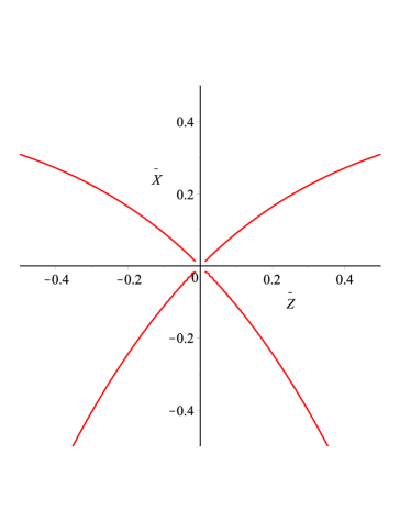
x   

Figure 1: Metric field values vs the electric potential values in phase space

References

- [1] R. M. Wald, ‘General relativity‘, The University of Chicago Press, Chicago and London, (1984).
- [2] B. Fauster, J. Tolksdorf and E. Zeidler,‘Quantum gravity, Mathematical Models and Experimental Bounds‘, Birkhauser Verlag, Basel, Switzerland, (2007).
- [3] L. Parker and D. Toms, ‘Quantum field theory in curved spacetime, Quantized fields and gravity‘,, Cambridge University press, (2009)
- [4] N. D. Birrel and P. C. W. Davies, ‘Quantum fields in curved space‘, Cambridge University press, (1982).
- [5] F. Bastianelli and P. Van. Nieuwenhuizen, ‘Path integrals and anomalies in curved space‘, Cambridge University Press, (2006).
- [6] B. Dewitt, ‘Quantum Theory of Gravity. I. The Canonical Theory‘. Phys. Rev.160, 1113, (1967).
- [7] P. V. Moniz, ‘Quantum cosmology-The supersymmetric perspective, Vol. 1 and 2‘, Springer-Verlag, Berlin, Heidelberg (2010).
- [8] C. Rovelli and F. Vidotto, ‘Covariant loop quantum gravity, an elementary introduction to quantum gravity and spinefoam theory‘, Cambridge University Press (2015).
- [9] B. Zwiebach, ‘A first course in string theory‘, Cambridge University Press (2004)
- [10] M. Gasperini, ‘Elements of stirng cosmology‘, Cambridge Univeristy Press (2007).
- [11] J. W. Barett, ‘Quantum gravity as topological quantum field theory‘, J.Math.Phys. 36 6161, (1995); arXiv:gr-qc/9506070
- [12] L. Freidel and A Starodubtsev, ‘Quantum gravity in terms of topological observables‘, arXiv:hep-th/0501191
- [13] S. W. Hawking, Nature (London) 248, 30 (1974)
- [14] S. W. Hawking Commun. Math. Phys. 43, 199 (1975)
- [15] G. t‘Hooft,‘How studying black hole theory may help us to quantise gravity ‘,arXiv:2211.10723 [gr-qc]
- [16] L. Hamaide and T. Torres, ‘Black hole information recovery from gravitational waves,‘ arXiv:2211.13736 [gr-qc]
- [17] R. C. Rubio, F. Di Filippo, S. Liberati, C. Pacilio and M. Visser, ‘Comment on Stability properties of Regular Black Holes‘, arXiv:2212.07458 [gr-qc]
- [18] K. Jusufi, ‘Avoidance of singularity during the gravitational collapse with string T-duality effects‘, Universe, 9, 41, (2023); arXiv:2301.03590 [gr-qc]
- [19] H. Ghaffarnejad, ‘Quantum field backreaction corrections and remanant stable evaporating Schwarzschild-de Sitter dynamical black hole‘, Phys. Rev. D75, 084009 (2007).
- [20] G. O. Neto, D. L. Canedo and G. A. Monerat, ‘Tunneling probability for the birth of universes with radiation, cosmological constant and an ad hoc potential ‘,arXiv:2301.05056 [gr-qc]
- [21] M. Motaharfar and P. Singh,‘Tunneling wavefunction proposal with loop quantum geometry effects‘, arXiv:2212.14065 [gr-qc]
- [22] T. P. Shestakova, ‘The birth of the Universe as a result of the change of the metric signature ‘,arXiv:2207.02689 [gr-qc]
- [23] H. Ghaffarnejad, ‘Quantum cosmology with effects of a preferred reference frame‘, Class. Quantum Gravit.27 (1), 015008 (2010).
- [24] E. N. Parker, ‘Cosmical magnetic fields‘ (Clarendon Press, Oxford, 1979)
- [25] Ya, B. Zeldovich, A.A. Ruzmaikin and D. D. Sokoloff, ‘Magnetic fields in Astrophysics‘, (Gordon and Breach, New York, 1983)
- [26] G. E. Zweibel and C. Heiles,‘Magnetic fields in galaxies and beyond‘, Nature volume 385, pages 131 (1997)
- [27] E. N. Parker, Astrophys. J. 163, 255 (1971)
- [28] A. Vilenkin and D. Leahy, Astrophys. J. 248, 13 (1981)
- [29] A. Vilenkin and D. Leahy, Astrophys. J. 254, 77 (1982)
- [30] C. Hogan, Phys. Rev. Lett. 51, 1488 (1983)
- [31] M. S. Turner and L. M. Widrow, ‘Inflation Produced, Large Scale Magnetic Fields‘, Phys.Rev. D 37, 2743 (1988).
- [32] H. Ghaffarnejad and L. Naderi, ‘Modified Gauge Invariance Einstein Maxwell Gravity and Stability of Spherical Stars with Magnetic Monopoles ‘, arXiv:2212.09485 [gr-qc]
- [33] S. Gasiorowicz, ‘Quantum mechanics‘, John Wiley and sons 1974.
- [34] L. Neslusan, ‘On the global electrostatic charge of stars‘, Astro. and Astrophys. 372, 913 (2001)
- [35] H. Ghaffarnejad, T. Ghorbani and F. Eidizadeh, ‘On the stability of electrostatic stars with modified non-gauge invariance, Einstein-Maxwell gravity ‘, arXiv:2301.00682 [gr-qc]
x