Core-corona procedure and microcanonical hadronization to understand strangeness enhancement in proton-proton and heavy ion collisions in the EPOS4 framework

Abstract

The multiplicity dependence of multistrange hadron yields in proton-proton and lead-lead collisions at several TeV allows one to study the transition from very big to very small systems, in particular, concerning collective effects. I investigate this, employing a core-corona approach based on new microcanonical hadronization procedures in the EPOS4 framework, as well as new methods allowing one to transform energy-momentum flow through freeze-out surfaces into invariant-mass elements. I try to disentangle effects due to “canonical suppression” and “core-corona separation”, which will both lead to a reduction of the yields at low multiplicity.

I Introduction

An enhancement of multistrange hadrons in relativistic heavy ion collisions compared with proton-proton scattering is one of the oldest signals proposed to detect the creation of a “quark-gluon plasma” [1]. It was observed first (as expected) in heavy ion collisions [2, 3, 4, 5, 6] but, unexpectedly, such “signals” have also been detected in proton-protons collisions, where the enhancement concerns high-multiplicity compared with low-multiplicity events [7]. Even more, when one plots ratios of multistrange hadrons to pions, as a function of the multiplicity $dn/d\eta$ at rapidity zero, for both proton-proton (at 7 TeV) and heavy ions (PbPb at 2.76 TeV), one observes a unique curve, increasing monotonically from low-multiplicity proton-proton up to central PbPb. Also shown in Ref. [7]: the standard Monte Carlo event generators do not really describe the data.

During the past five years, the EPOS4 project was developed (see first publications [8, 9, 10]), being an attempt to construct a realistic model for describing relativistic collisions of different systems (from proton-proton to nucleus-nucleus) at energies from several GeV per nucleon up to several TeV. So the model should be able to deal with strangeness enhancement, but not only. It is a “general purpose” approach that is meant to describe any observable. The results shown in this paper are only a very small fraction of simulation results, since as a first test of the new approach simulations were performed at low energies, i.e., 7.7, 11.5, 14.5, 19.6, 27, 39, 62.4, 130, and 200 GeV / nucleon, and as well at high energies, i.e., 2.76, 5.02, 7, 8, 13 TeV / nucleon, for different systems, looking for yields, spectra, and flow, for light and heavy flavor. All this is done with the same code version, namely EPOS4.0.0, which is at this moment being published via a dedicated web page. No attempt has been made to “fit” one particular curve for one particular system, the idea is more to see to what extent one understands the enormous amount of data accumulated over the past two decades.

A fundamental ingredient of the EPOS4 approach is the observation that multiple (nucleonic or partonic) scatterings must happen in parallel, and not sequentially, based on very elementary considerations concerning time-scales. To take this into account, EPOS4 brings together ancient knowledge about S-matrix theory (to deal with parallel scatterings) and modern concepts of perturbative QCD and saturation, going much beyond the usual factorization approach. The parallel scattering principle requires sophisticated Monte Carlo techniques, inspired by those used in statistical physics to investigate the Ising model.

In the EPOS4 approach, one distinguishes “primary scatterings” and “secondary scatterings”. The former refer to the above-mentioned parallel scatterings with the initial nucleons (and their partonic constituents) being involved, happening at very high energies instantaneously. The theoretical tool is S-matrix theory, using a particular form of the proton-proton scattering S-matrix ( Gribov-Regge approach [11, 12, 13, 14]), which can be straighforwardly generalized to be used for nucleus-nucleus collisions. Although these basic assumptions are not only well-motivated, but also very simple and transparent, the practical application is complicated. This is due to the fact that when developing matrix elements in terms of multiple scattering diagrams, the large majority of the diagrams cancel when it comes to inclusive cross sections. But in EPOS4 one keeps all contributions since one wants to go beyond inclusive cross sections (important when studying high multiplicity events). The challenge for EPOS4 is to use the full parallel scattering scenario, but in a smart way such that for inclusive cross section the cancellations actually work. This is the new part in EPOS4, strongly based on an interplay between parallel scatterings and saturation. This is discussed in detail in separate publications [8, 9, 10]. Our S-matrix approach has a modular structure, it is based on so-called “Pomerons” (representing elementary parton-parton scatterings), and these Pomerons are constructed based on “parton ladders”, which makes the link to perturbative QCD. Also, this part has been completely redone, with particular care concerning the role of heavy flavor [9].

In this paper, I want to focus on the secondary scatterings, and in particular on the hadronization of “plasma droplets”. In Sec . II, I summarize briefly the “parallel scattering approach” for primary scatterings. In Sec . III, I discuss how the EPOS4 multiple-scattering diagrams translate into particle production, which means first the production of so-called prehadrons,which may originate from Pomerons or from remnants. Based one these prehadrons, a core-corona procedure will be employed, which allows one to identify the “core”, which will then be treated as a fluid which evolves and eventually decays into hadrons. In Sec. IV, I discuss the main topic of this paper, namely the hadronization of the core.

II Parallel scattering scenario in EPOS4

Let me briefly summarize the EPOS4 approach, considering first high-energy collisions, where a parallel scattering approach for primary scatterings is mandatory, in AA collisions but also concerning multiple partonic scatterings in pp reactions. In Refs. [8, 9, 10], it is shown in detail how such a “parallel scattering scheme” can be constructed rigorously based on S-matrix theory, which will be sketched in the following.

The starting point is the elastic-scattering T-matrix $T$ for pp scattering, expressed as a product of “elementary” T-matrices $T_{\mathrm{Pom}}$ representing parton-parton scattering via Pomeron exchange. The expression can be easily generalized for AA scattering. In both cases, pp or AA, this formalism allows a strict parallel scattering picture. The precise content of the Pomerons will be discussed later. The connection with inelastic scattering provides the optical theorem, using so-called cutting rules, which allows one to express the total cross section (which by definition adds up all inelastic processes) in terms “cut Pomerons” $G$, as shown for the case of two inelastic scatterings in Fig. 1.

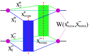
Figure 1: Double scattering, each box representing a cut Pomeron $G$ (single inelastic scattering).

The light-cone momentum fractions $x^{+}$ and $x^{-}$ are shared between the two Pomerons and the remnants ($W$ in the plot represents some vertex function). Each cut Pomeron $G$ represents a squared amplitude of a single inelastic scattering.

The important new issue in Ref. [8, 9, 10] is the understanding of how energy conservation ruins factorization (which strictly speaking makes the model inapplicable), and how to solve the problem via an appropriate definition of $G$. The cut Pomeron, representing a single inelastic scattering is the fundamental quantity in the EPOS formalism. For the moment, one considers the Pomeron as a “box” (the precise internal structure will be discussed later), with two external legs representing two incoming partons carrying light-cone momentum fractions $x^{+}$ and $x^{-}$, so $G=G(x^{+},x^{-},s,b)$, with the energy squared $s$, and the impact parameter $b$, see Fig. 2.

$$\boldsymbol{\boldsymbol{=G(x^{+},x^{-},s,b)}}$$

Figure 2: The cut Pomeron $G$.

Let me define the “Pomeron energy fraction” $x_{\mathrm{PE}}=x^{+}x^{-}=M_{\mathrm{Pom}}^{2}/s,$ with $M_{\mathrm{Pom}}$ being the transverse mass of the Pomeron, which is the crucial variable characterizing cut Pomerons: the bigger $x_{\mathrm{PE}}$, the bigger the Pomeron’s invariant mass and the number of produced particles. Large invariant masses also favor high-$p_{t}$ jet production.

Let me consider a AA collision (including pp as a special case). I define, for a given cut Pomeron connected to projectile nucleon $i$ and target nucleon $j$, a “connection number” $N_{\mathrm{conn}}=(N_{\mathrm{P}}+N_{\mathrm{T}})/2,$ with $N_{\mathrm{P}}$ being the number of Pomerons connected to i, and with $N_{\mathrm{T}}$ being the number of Pomerons connected to j. The case $N_{\mathrm{conn}}=1$ corresponds to an isolated Pomeron, which may take all the energy of the initial nucleons, whereas in case of $N_{\mathrm{conn}}>1$ the energy will be shared. To quantify the effect of the energy sharing, one defines $f^{(N_{\mathrm{conn}})}(x_{\mathrm{PE}}$) to be the inclusive $x_{\mathrm{PE}}$ distribution, i.e. the probability that a single Pomeron carries an energy fraction $x_{\mathrm{PE}}$, for Pomerons with given values of $N_{\mathrm{conn}}$. The main problem which ruins factorization is the fact that the distribution for $N_{\mathrm{conn}}>1$ will be deformed with respect to the $N_{\mathrm{conn}}=1$ case, due to energy sharing. I define the corresponding “deformation function” $R_{\mathrm{deform}}(x_{\mathrm{PE}})$ as a ratio of $f^{(N_{\mathrm{conn}})}(x_{\mathrm{PE}}$) over $f^{(1)}(x_{\mathrm{PE}}$). I also use the notation $R_{\mathrm{deform}}^{(N_{\mathrm{conn}})}(x_{\mathrm{PE}})$ to undeline its $N_{\mathrm{conn}}$ dependence. As shown in Refs. [8, 10], this function can be calculated and tabulated. As discussed in very much detail in Ref. [9], one also calculates and tabulate some function $G_{\mathrm{QCD}}(Q^{2},\,x^{+},x^{-},s,b)$, which contains as a basic element a cut parton ladder based on Dokshitzer-Gribov-Lipatov-Altarelli-Parisi (DGLAP) parton evolutions [13, 15, 16] from the projectile and target side, with an elementary QCD cross section in the middle, $Q^{2}$ being the low virtuality cutoff in the DGLAP evolution. The latter is usually taken to be constant and of the order of $1\,$GeV, whereas here one allows any value. With all this preparation, one is now able to connect $G$ (used in the multi-Pomeron diagrams) and $G_{\mathrm{QCD}}$ [which contains all the perturbative QCD (pQCD) diagrams], as follows: For each cut Pomeron, for given $x^{\pm}$, $s$, $b$, and $N_{\mathrm{conn}}$, one postulates:

$$G(\!\,x^{+}\!\!,x^{-}\!\!,s,b)\!=\frac{n}{R_{\mathrm{deform}}^{(N_{\mathrm{conn}})}(x_{\mathrm{PE}})}G_{\mathrm{QCD}}(Q_{\mathrm{sat}}^{2}\,,\,x^{+}\!\!,x^{-}\!\!,s,b),$$ (1)

with

$$G\;\mathrm{independent}\;\mathrm{of}\;N_{\mathrm{conn}}.$$ (2)

But $Q_{\mathrm{sat}}^{2}$ does depend on $N_{\mathrm{conn}}$ (and also on $x^{\pm}$). The symbol $n$ is a factor not depending on $x^{\pm}$. This is the fundamental equation in the new EPOS4 approach. As shown in Refs. [8, 10], this deformation in the denominator of Eq. (1) corrects perfectly the deformation of the $x_{\mathrm{PE}}$ distribution, the only effect of energy sharing is a modification of $Q_{\mathrm{sat}}^{2}$, and the latter will only affect low-$p_{t}$ processes. In this way, one recovers factorization, and binary scaling in AA (with $R_{AA}=1$) at large transverse momenta for inclusive cross sections (but only for them). In other words, at large $p_{t}$, the full multiple-scattering machinery produces exactly the same result as compared with simply taking one single Pomeron (single scattering), which allows one to define and compute (in the EPOS framework) parton distribution function, tabulate them, and then compute inclusive jet cross sections based on these (using standard procedures).

But such a “shortcut” (also referred to as “EPOS4 factorization mode”) is only possible for inclusive cross sections, and only at high $p_{t}$. But this represents only a very small fraction of all possible applications, and there are very interesting cases outside the applicability of that approach. A prominent example, one of the highlights of the past decade in our domain, concerns collective phenomena in small systems. It has been shown that high-multiplicity pp events show very similar collective features as earlier observed in heavy ion collisions [17]. High multiplicity means automatically “multiple parton scattering”. As discussed earlier, this means that one has to employ the full parallel scattering machinery developed earlier, based on S-matrix theory. One cannot use the usual parton distribution functions (representing the partonic structure of a fast nucleon), one has to treat the different scatterings (happening in parallel) individually, and for each scattering, one has a parton evolution according to some evolution function $E$ (representing the partonic structure of a fast parton), as sketched in Fig. 3.

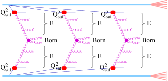
Figure 3: Rigorous parallel scattering scenario, for $n=3$ parallel scatterings, including non-linear effects via saturation scales. The red symbols should remind one that the parts of the diagram representing nonlinear effects are replaced by simply using saturation scales.

One still has DGLAP evolution, for each of the scatterings, but one introduces saturation scales. But, most importantly, these scales are not constants, they depend on the number of scatterings, and they depend as well on $x^{+}$ and $x^{-}$. An example of a multiple-scattering AA configuration is shown in Fig. 4.

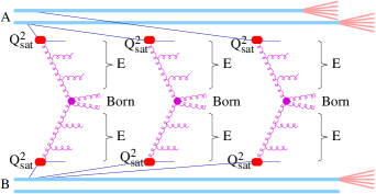
Figure 4: Rigorous parallel scattering scenario, for $n=3$ parallel scatterings for a collision of a nucleus $A$ with a nucleus $B$ , including non-linear effects via saturation scales.

The diagrams shown in Figs. 3 and 4 are meant to be “symbolic”, the real structure is somewhat more complex. Also for simplicity, one consider only gluons in the diagrams. I also do not consider (for simplicity) timelike parton emissions, but in the real EPOS4 simulations they are of course taken care of, based on angular ordering. For a complete description, see Ref. [9].

But all this “multiple-scattering discussion” is not the full story. The S-matrix part concerns “primary scatterings”, happening instantaneously at $t=0$. As a result, in the case of a large number of Pomerons, one has correspondingly a large number of “prehadrons”, and based on these, “secondary interactions” occur: fluid formation and decay and hadronic rescatterings. This will be discussed in the next section.

III The role of core, corona, and remnants

In this section, I will discuss briefly how the EPOS4 multiple scattering diagrams translate into particle production, which means first the production of so-called prehadrons. As discussed below, our Pomerons are mapped into kinky relativistic strings, where string decay traditionally produces string segments which correspond to hadrons. But one considers the possibility of having a dense environment, and here the string segments cannot “evolve” into hadrons. So one uses the term “prehadrons” for these segments, and they either “fuse” to produce the core, or become hadrons if they escape the core. A similar argument is used for excited remnants, which may decay into hadrons, but again this may happen in a dense area. In Ref. [9], one discusses the different types of Pomerons and their relation with pQCD, including technical details for the computations, and one also discusses how the pQCD diagrams translate into kinky strings. String decay into segments (now called prehadrons) is disussed in detail in Ref. [18]. Based on these prehadrons, a core-corona procedure will be employed, which allows identifying the “core”, which will then be treated as a fluid that evolves and eventually decays into hadrons, which still may collide with each other.

In Fig. 5, I consider an example of a multiple cut Pomeron (i.e. multiple scattering) configuration of two colliding nuclei $A$ and $B$ at Large Hadron Collider (LHC) energies (several TeV), each nucleus composed of two nucleons (just for illustration). Dark blue lines mark active quarks, red dashed lines active antiquarks, and light blue thick lines projectile and target remnants (nucleons minus the active (anti)quarks). I have chosen an example with two scatterings of “sea-sea” type, and one of “val-sea” type (see Ref. [9]). One considers each incident nucleon as a reservoir of three valence quarks plus quark-antiquark pairs. The “objects” which represent the “external legs” of the individual scatterings are colorless: quark-antiquark pairs in most cases as shown in the figure, but one may as well have quark-diquark pairs or even antiquark-antidiquark pairs – in any case, a $3$ and a $\bar{3}$ color representation. In general, each of the horizontal gluon lines would develop the so-called

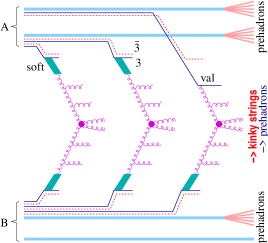
Figure 5: Multiple scattering configuration of two colliding nuclei $A$ and $B$ at LHC energies, each nucleus being composed of two nucleons, with three scatterings (from three cut Pomerons). Dark blue lines mark active quarks, red dashed lines active antiquarks, and light blue thick lines projectile and target remnants. One of the target nucleons is just a spectator.

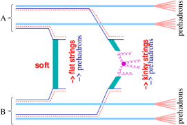
Figure 6: As Fig. 5, but for lower energy.

timelike cascade, which is not considered here for the simplicity of the discussion. I also consider only gluons here, in general, there are as well $g\to q+\bar{q}$ splittings. This multiple-scattering picture works perfectly also at lower energies [BNL Relativistic Heavy Ion Collider (RHIC)]. With decreasing energy, it becomes simply more and more likely that the Pomerons in Fig. 5 are replaced by purely soft ones, as indicated in Fig. 6. Also the Pomerons get less energetic, producing fewer particles.

For a given diagram as for example Fig. 5, one constructs the corresponding color flow diagram (two arrows per gluon, forward and backward arrows for quarks and antiquarks). One then follows the color flow arrows, for example starting with a $\bar{3}$ being an external leg on the projectile side, until one finds a $3$ which is in our example an external leg on the target side. This defines a chain of partons. Assuming that the external legs are simply quarks and antiquarks, one gets six chains of the type $\bar{q}-g-g-...-g-q$, mapped (in a unique fashion) to kinky strings, where each parton corresponds to a kink. This is explained in detail in Ref. [9]. The kinky strings are then decayed into prehadrons.

A second source of particle production are the remnants. In case of multiple scattering as in Fig. 5, the projectile and target remnants remain colorless, but they may change their flavor content during the multiple collisions. The quark-antiquark pair “taken out” for a collision (the “external legs” for the individual collisions), may be $u$-$\bar{s}$, then the remnant for an incident proton has flavor $uds$. In addition, the remnants get massive, much more than a simply resonance excitation. One may have remnants with masses of $10\,\mathrm{GeV/c^{2}}$ or more, which contribute significantly to particle production (at large rapidities).

In the above discussion, I mentioned the production of “prehadrons” from strings and from remnant decays. Based on these prehadrons, one employs a so-called core-corona procedure (introduced in Ref. [19], updated in Ref. [20]), at some given (early) proper-time $\tau_{0}$, see Fig. 7.

(a)                                    (b)                                             
            

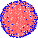
Figure 7: Sketch of the core-corona separation for a “big” (a) and a “small” (b) system. The dots are prehadrons in the transverse plane, red refers to core, blue to corona.

The method is used for all systems, big ones (as central AA) or small ones (peripheral AA, or even pp scattering). One considers all prehadrons at $\tau_{0}$, marked as dots in Fig. 7. For each prehadron, one computes

$$p_{t}^{\mathrm{new}}=p_{t}-0.25\big{(}f_{\mathrm{EL1}}\!+\!Z(f_{\mathrm{EL2}}\!-\!f_{\mathrm{EL1}})\big{)}p_{t}^{g_{\mathrm{EL}}}\!\!\int_{\gamma}\rho^{h_{\mathrm{EL}}}\,dL,$$ (3)

where $\gamma$ is the trajectory of the prehadron moving out of the system, and $Z=(N_{\mathrm{part}}-2)/N_{\mathrm{part}}^{\mathrm{max}}$ the “centrality” based on the number of participants. I define “cone prehadrons” as prehadrons within a jet cone radius $R$ with respect to a parton with $p_{t}\geq 1\,$GeV/c, considering all the partons which constitute the kinky string being the origin of the prehadron in question. All others are “noncone prehadrons”. The jet cone radius is defined as $R^{2}=(\Delta\eta)^{2}+(\Delta\phi)^{2}$, with $\Delta\eta$ and $\Delta\phi$ being respectively the difference in pseudorapidity and azimuthal angle, with respect to the parton. I use jet cone radii of 0.3 (pp) and 0.2 (PbPb). I use different sets of parameters $\{f_{\mathrm{EL1}},f_{\mathrm{EL2}},g_{\mathrm{EL}},h_{\mathrm{EL}}\}$ for noncone and cone prehadrons, namely, $\{0.1,-,0.5,0.375\}$ (pp cone), $\{0.4,-,0,1\}$ (pp noncone), $\{0.3,0.3,0.5,0.375\}$ (PbPb cone), $\{0.5,0.7,0,1\}$ (PbPb noncone). The prehadron in question is then considered to be of “core” or “corona” type, based on the following criteria:

• For $p_{t}^{\mathrm{new}}\leq 0$, the prehadron is considered to be a “core prehadron”.

• For $p_{t}^{\mathrm{new}}>0$, the prehadron escapes, it is called “corona prehadron”.

The core prehadrons constitute “bulk matter” and will be treated via hydrodynamics. The corona prehadrons become simply hadrons and propagate with reduced energy (due to the energy loss). In Fig. 7, I distinguish between big and small systems. Actually, the method used is the same, but there are relatively more core prehadrons in the big systems. Corona particles are either very energetic (then they move out even from the center), or they are close to the surface, or one has a combination of both.

The core-corona procedure is a crucial element in the EPOS4 approach, which allows soft and hard elements to emerge naturally from a unique formalism (rather than constructing a two-component approach). It is also important to understand that a hard process (in the usual terminology), which is in the EPOS4 framework a high transverse momentum pQCD process, will also contribute to low-$p_{t}$ particle production, since only string breaks close to the the high-$p_{t}$ kink will produce high-$p_{t}$ particles.

The importance of the core-corona picture is also emphasized in Refs. [21], [22], and [23].

Let me investigate the core-corona effects in EPOS4 first for proton-proton collisions. One wants to understand the relative importance of the core part, and one also wants to know which fraction is coming from remnant decay.

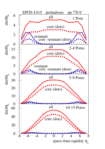
Figure 8: The prehadron yield as a function of space-time rapidity, for different Pomeron numbers in proton-proton collisions at 7 TeV. The curves refer to all prehadrons (red full), all core prehadrons (red dotted), prehadrons from remnant decay (blue full), and core prehadrons from remnant decay (blue dotted).

In Fig. 8, I show results for different event classes (defined via Pomeron numbers) in proton-proton collisions at 7 TeV. I show in each case four different curves: all prehadrons (red full), all core prehadrons (red dotted), prehadrons from remnant decay (blue full), and core prehadrons from remnant decay (blue dotted). Not too surprisingly, remnant contributions show up in general at large rapidities, but in all cases they do contribute to the core. Comparing the red full and dotted curves, one sees that the core fraction is in all cases substantial, most significantly for the event class “10-15 Pomerons”, but even for small Pomeron numbers, the core contribution remains important. As a small side remark: it is often said that “collectivity” is seen in high multiplicity pp scattering. In our EPOS4 analysis, it is even essential in minimum bias collisions (with an average Pomeron number of around 2), very strongly supported by data.

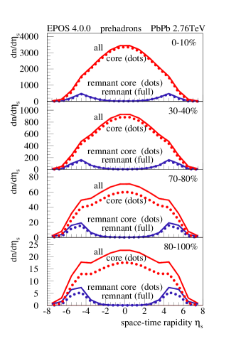
Figure 9: The prehadron yield as a function of space-time rapidity, for different centralities in PbPb collisions at 2.76 TeV. The curves refer to all prehadrons (red full), all core prehadrons (red dotted), prehadrons from remnant decay (blue full), and core prehadrons from remnant decay (blue dotted).

Let me now turn to AA scattering, to understand the relative importance of the core part, and of the fraction coming from remnant decay. In Fig. 9, I show results for different centralities in PbPb collisions at 2.76 TeV, namely (from top to bottom): 0-10%, 30-40%, 70-80%, and 80-100% (based on the distribution of the impact parameter). Also here, the remnant contributions show up preferentially at large rapidities, and in all cases, they do contribute to the core. Comparing the red full and dotted curves, one sees that the core fraction (ratio of $dn/d\eta_{s}$ of the core contribution over all) is in all cases substantial: 0.97 for 0-10%, 0.95 for 30-40%, 0.85 for 70-80%, and 0.77 for 80-100%. One also sees that this “core dominance” extends over a wide rapidity range.

Having identified core pre-hadrons, one computes the corresponding energy-momentum tensor $T^{\mu\nu}$ and the flavor flow vector at some position $x$ at initial proper time $\tau=\tau_{0}$ as

$$T^{\mu\nu}(x)=\sum_{i}\frac{p_{i}^{\mu}p_{i}^{\nu}}{p_{i}^{0}}g(x-x_{i})$$ (4)

and

$$N_{q}^{\mu}(x)=\sum_{i}\frac{p_{i}^{\mu}}{p_{i}^{0}}\,q_{i}\,g(x-x_{i}),$$ (5)

with $q_{i}\in\{u,d,s\}$ being the net flavor content and $p_{i}$ the four-momentum of prehadron $i$. The function $g$ is a Gaussian smoothing kernel, in Milne coordinates given as $g(x)=h(\eta/d_{\|})h(x/d_{\bot})h(y/d_{\bot})$, with $h(s)=\frac{1}{\sqrt{2\pi}}\exp(-\frac{1}{2}s^{2})$, with parameters $d_{\|}$ and $d_{\bot}$.

The parameter $d_{\|}$ is given as $\min(1.0,r(s))$, with $r(s)=\max(0.5,y(s)/y(s_{\mathrm{ref}}))$, where $y(s)$ is the rapidity of the projectile nucleons in the nucleon-nucleon center-of-mass for a squared nucleon-nucleon energy $s$, and where $s_{\mathrm{ref}}=(2.76\mathrm{TeV)^{2}}$ is some reference value. The parameter $d_{\bot}$ is given as $0.3+0.3Z$ for PbPb and as $0.3-0.02\min(N_{\mathrm{Pom}}-1,12)$ for pp, where $Z=(N_{\mathrm{part}}-2)/N_{\mathrm{part}}^{\mathrm{max}}$ is the centrality based on the number of participants and $N_{\mathrm{Pom}}$ the number of (cut) Pomerons (characterizing the event activity in pp).

The Lorentz transformation of $T^{\mu\nu}$ into the comoving frame provides the energy density $\varepsilon$ and the flow velocity components $v^{i}$, which will be used as the initial condition for a hydrodynamical evolution [20]. This is based on the hypothesis that equilibration

Figure 10: Energy density at the initial proper-time $\tau_{0}$ as a function of the transverse coordinate $r$. The full red lines correspond to an azimuthal angle $\phi=0$, and the dotted red lines to $\phi=\pi/2$. The blue dashed lines represent the freeze-out energy density. I show results for different event classes (defined via Pomeron numbers) in pp collisions at 7 TeV (upper plot) and for different centralities (defined via impact parameter) in PbPb collisions at 2.76 TeV (lower plot).

happens rapidly and affects essentially the space components of the energy-momentum tensor. In Fig. 10 (upper plot), I show the energy density at the initial proper-time $\tau_{0}$ as a function of the transverse coordinate $r$ for different event classes (defined via Pomeron numbers) in pp collisions at 7 TeV. The values of $\tau_{0}$ is $0.4\,$fm/c in EPOS4.0.0. I also indicate in the figure the freeze-out energy density (blue dashed line). For each event, one determines (based on the energy density distribution) the event plane angle $\psi$ and rotate the system accordingly (to have after rotation event plane angles zero). The plots in Fig. 10 represent averages over such rotated events, the full lines correspond to azimuthal angles $\phi=0$, the dotted lines to $\phi=\pi/2$. The difference between the two lines reflects the azimuthal asymmetry. As already seen in Fig. 8, even in the case of a single Pomeron, there is some core production, and one gets actually an energy density of several $\mathrm{GeV/fm^{3}}$, but the radial extension is very small, and the lifetime (before freeze-out) very small. For large Pomeron numbers, the energy densities and the radial extensions get bigger, but the latter remain of the order of 1 $\mathrm{fm/c}$.

In Fig. 10 (lower plot), I show the energy density at the initial proper-time $\tau_{0}$ as a function of the transverse coordinate $r$ for different centralities (defined via impact parameter) in PbPb collisions at 2.76 TeV. The values of $\tau_{0}$ are between $2\,$fm/c and $1\,$fm/c from central to peripheral in EPOS4.0.0. Also here one does the rotations according to the event plane angles, as discussed above for pp scattering, before taking event averages. Based on these, the full lines correspond to azimuthal angles $\phi=0$, the dotted line to $\phi=\pi/2$. As already seen in Fig. 9, even in peripheral collisions, there is some core production, and one gets actually an energy density of about $\mathrm{2\,GeV/fm^{3}}$ for 70-80% centrality, but the radial extension is small, and the lifetime as well.

It follows a viscous hydrodynamic expansion. Starting from the initial proper time $\tau_{0}$, the core part of the system evolves according to the equations of relativistic viscous hydrodynamics [20, 24], where one uses presently $\eta/s=0.08$. The “core-matter” hadronizes on some hyper-surface defined by a constant energy density $\epsilon_{H}$ (presently $0.57\mathrm{\,GeV/fm^{3}}$). In earlier versions [25], one used a so-called Cooper-Frye procedure. This is problematic in particular for small systems: not only do energy and flavor conservation become important, but one also encounters problems due to the fact that one gets small “droplets” with huge baryon chemical potential, with strange results for heavy baryons. In EPOS4, one systematically uses microcanonical hadronization, with major technical improvements compared to earlier versions, as I will discuss below.

IV Microcanonical hadronization of the core

In EPOS4, one systematically uses micro-canonical hadronization. Due to several technical improvements, our procedures work for all kinds of systems (big and small ones), and one uses it for proton-proton as well as heavy ion scattering. But not only for technical reasons. The usual Cooper-Frye procedure amounts to a smooth transition from a fluid to a particle description. However, one has a violently expanding system into the vacuum, where around some critical energy density the system goes very quickly from one state (plasma) to a very different one (hadrons), in a complicated fashion. So one assumes – whatever the precise mechanism might be – that the system decays into multi-hadron states, randomly. And the most random way corresponds to maximizing the entropy, which amounts to the micro-canonical ensemble. Being a crucial element of the new EPOS4 approach, I will discuss this in the following.

It is important to note that

• there is no need to match the dynamical part of hydro evolution, one considers a sudden statistical decay

• one has full energy and flavor conservation, which is important for small systems

• the procedure is extremely fast, and can be used for “big systems” and in particular study the limiting case of “very large plasma droplets” (infinite volume limit).

IV.1 Infinite volume limit

Let me first look at the infinite volume limit, which is the grand canonical ensemble. Here, for single particle spectra (particle species $k$), one has the distribution

$$f_{k}=\frac{g_{k}V}{(2\pi\hbar)^{3}}\,\exp\left(-\frac{E_{k}}{T}\right),$$ (6)

with degeneracy $g_{k}$, volume $V$, energy $E_{k}$ and temperature $T$. The average energy is

$$\left\langle E\right\rangle=\sum_{k}\frac{g_{k}V}{(2\pi\hbar)^{3}}\int_{0}^{\infty}E_{k}\exp\left(-\frac{E_{k}}{T}\right)4\pi p^{2}dp,$$ (7)

Changing variables via $E_{k}dE_{k}=pdp$, and using

$$K_{1}(z)=z\int_{1}^{\infty}\exp(-zx)\sqrt{x^{2}-1}dx,$$ (8)

$$3\,K_{2}(z)=z^{2}\int_{1}^{\infty}\exp(-zx)\sqrt{x^{2}-1}^{3}dx,$$ (9)

one gets

$$\left\langle E\right\rangle=\sum_{k}\frac{4\pi g_{k}V}{(2\pi\hbar)^{3}}m_{k}^{2}T\left(3TK_{2}(\frac{m_{k}}{T})+m_{k}K_{1}(\frac{m_{k}}{T})\right).$$ (10)

This formula allows one to compare micro-canonical and grand-canonical decay using the same average energy (this will be done later). Generating hadrons according to Eq. (6), onev may compute the total energy $E$ of the produced particles, and then compare with the average energy $\left\langle E\right\rangle$, Eq. (10).

Figure 11: The distribution of $X=E/\left\langle E\right\rangle$, i.e. the ratio of final energy over initial energy, for a temperature of 130 MeV and volumes $V=50\,$fm³ (red curve) and $V=1000\,$fm³ (blue dashed curve).

In Fig. 11, I plot the distribution of $E/\left\langle E\right\rangle$, for a temperature of 130 MeV and two values for the volume $V$, namely V=50 fm³ and V=1000 fm³. This shows the amount of violation of energy conservation, which increases with decreasing volume.

IV.2 Microcanonical hadronization of plasma droplets

Let me now turn to micro-canonical decay of a “plasma droplet” of volume $V$ and energy $E$ (also referred to as mass $M$). Here, all the states are equally probable, so the weight of a decay of the droplet in its center-of-mass system (CMS into $n$ hadrons with momenta $\vec{p}_{i}$ is given as

$$dP\boldsymbol{=}C_{\textrm{vol}}\,C_{\textrm{deg}}\,C_{\textrm{ident}}\,d\Phi_{\mathrm{NRPS}},$$ (11)

with the constants (the indices referring to volume, degeneracy, and identical particles)

$$C_{\textrm{vol}}=\frac{V^{n}}{(2\pi\hbar)^{3n}}\,\,,\,\,\,\,C_{\textrm{deg}}=\prod_{i=1}^{n}g_{i}\,\,,\,\,\,\,C_{\textrm{ident}}=\prod_{\alpha\in\mathcal{S}}{\frac{1}{n_{\alpha}!}}\,\,,$$ (12)

and with

$$d\Phi_{\mathrm{NRPS}}=\delta(E-\Sigma E_{i})\,\delta(\Sigma\vec{p}_{i})\,\prod_{A}\delta_{Q_{A},\Sigma q_{A\,i}}\,\prod_{i=1}^{n}d^{3}p_{i}\,,$$ (13)

with $E_{i}=\sqrt{m_{i}^{2}+p_{i}^{2}}$ being the energy and $\vec{p}_{i}$ the 3-momentum of particle $i$. Here, $C_{\textrm{deg}}$ accounts for degeneracies ($g_{i}$ is the degeneracy of particle $i$), and $C_{\textrm{ident}}$ accounts for the occurrence of identical particles ($n_{\alpha}$ is the number of particles of species $\alpha$). The term $\delta_{Q_{A},\Sigma q_{A\,i}}$ reflects conservation laws (baryon ($A=B$), electric charge ($A=C$) and strangeness ($A=S$). It should be noted that one has to use the “non-relativistic phase space (NRPS)” $d\Phi_{\mathrm{NRPS}}$ rather than the Lorentz-invariant phase space (LIPS) $d\Phi_{\mathrm{LIPS}}$ used for the decay of massive particles, where asymptotic states are defined over an infinitely large volume, whereas here one considers a finite volume (see discussion in Ref. [26]). But of course, one uses the relativistic expressions $E_{i}=\sqrt{p_{i}^{2}+m_{i}^{2}}$ for hadron energies.

Numerical procedures to deal with these n-body phase-space expressions are quite involved, and have a long history. Cerulus and Hagedorn [27] provided in 1958 a way to evaluate the NRPS integrals $\Phi_{\mathrm{NRPS}}=\int d\Phi_{\mathrm{NRPS}}$, which they used to compute particle production in high energy collisions. Shortly after it was proposed to better use a covariant formula, referred to as the Lorentz-invariant phase-space (LIPS) integral. The corresponding algorithms for Monte Carlo applications were discussed by James [28] in 1968 and heavily used for computing particle production. Being still relevant concerning the decay of a quark gluon plasma, the NRPS integrals and the corresponding Hagedorn prescriptions were used for Monte Carlo realizations (Werner and Aichelin [29] in 1994, Becattini and Ferroni [26] in 2004) of particle production in heavy ion collisions. In 2012 (Bignamini et al. [30]), it was proposed to use the fact that the non-relativistic phase-space (NRPS) element is up to a factor equal to the Lorentz invariant phase-space (LIPS) element, which is much easier to handle for $n$ not too large.

The Cerulus-Hagedorn method employed in Ref. [29] is not very efficient and needs enormous computing efforts at intermediate $n$ (around $n=10$) and at very large $n$, whereas the LIPS method employed in Ref. [30] works well at small $n$, but gets very time consuming at large $n$.

I will employ a hybrid method, i.e. an improved (and very efficient) Cerulus-Hagedorn method for large $n$, and the LIPS method for small $n$, such that one has finally very efficient procedures for any $n$, even for very big values (for very big plasma droplets).

Let me first discuss the “improved Cerulus-Hagedorn method”. Cerulus and Hagedorn [27] proposed to write the phase-space integral as

$$\Phi_{\mathrm{NRPS}}=(4\pi)^{n}\int\prod_{i=1}^{n}p_{i}^{2}\,\delta(E-\sum_{i=1}^{n}E_{i})\,W(p_{1},\ldots,p_{n})\prod_{i=1}^{n}dp_{i},$$ (14)

with $p_{i}=\left|\vec{p}_{i}\right|$, and with the “random walk function” $W$ (also called angular integral)

$$W(p_{1},\ldots,p_{n}):=\frac{1}{(4\pi)^{n}}\int\delta\big{(}\sum_{i=1}^{n}p_{i}\vec{u}_{i}\big{)}\prod_{i=1}^{n}d\Omega_{i}\,,$$ (15)

with $\vec{u}_{i}=\vec{p}_{i}/p_{i}$ and $\Omega_{i}$ referring to the corresponding solid angle. The crucial point is an efficient calculation of the angular integral $W$. It may be written as (omitting the arguments $p_{1},\ldots,p_{n}$)

$$W=\frac{1}{(4\pi)^{n}}\frac{1}{(2\pi)^{3}}\int\int e^{-i\vec{\lambda}\Sigma p_{j}\vec{u}_{j}}\,\prod_{j=1}^{n}d\Omega_{j}\,d^{3}\lambda,$$ (16)

which leads to

$$W=\int_{0}^{\infty}F(\lambda)\,d\lambda,$$ (17)

with the integrand being

$$F(\lambda)=\frac{\lambda^{2}}{2\pi^{2}}\,\prod_{j=1}^{n}\frac{\sin p_{j}\lambda}{p_{j}\lambda}=\frac{\lambda^{2}}{2\pi^{2}}\,\prod_{j=1}^{n}\frac{\sin\pi{a}_{j}}{\pi{a}_{j}},$$ (18)

with $a_{j}=p_{j}\frac{\lambda}{\pi}$. One may use Euler’s product formula to get

$$\prod_{j=1}^{n}\frac{\sin\pi{a}_{j}}{\pi{a}_{j}}=\prod_{j=1}^{n}\prod_{k=1}^{\infty}\left(1-\frac{a_{j}^{2}}{k^{2}}\right),$$ (19)

which is for large $n$ approximately equal to

$$\exp\left(-{\frac{\pi^{2}}{6}}\sum_{j=1}^{n}a_{j}^{2}\right)$$ (20)

(having used $\sum_{k=1}^{\infty}\frac{1}{k^{2}}=\frac{\pi^{2}}{6}$). This means that the expression $\prod_{j=1}^{n}\{\sin p_{j}\lambda/p_{j}\lambda\}$ is well approximated by

$$\exp\left(-P^{2}\lambda^{2}\right),\quad\mathrm{with}\;P=\sqrt{\frac{1}{6}\sum_{j=1}^{n}p_{j}^{\>2}}.$$ (21)

The crucial point is the following: although this “approximation” is not precise enough to be used directly, one may use the fact that one has a rough estimate of the integrand $F(\lambda)$ to make a variable transformation which allows one to make a very accurate and efficient numerical integration. Thanks to the approxmation $F(\lambda)\approx\frac{\lambda^{2}}{2\pi^{2}}\exp\left(-P^{2}\lambda^{2}\right)$, one knows that

$$F_{0}(\lambda)=F(\lambda)\times\exp\left(P^{2}\lambda^{2}\right)$$ (22)

is a slowly varying function of $\lambda$ (polynomial dependence). The angular integral may then be written as

$$W=\int_{0}^{\infty}F(\lambda)\,d\lambda=\frac{1}{P}\int_{0}^{\infty}F_{0}\left(\frac{x}{P}\right)\,\times\exp\left(-x^{2}\right)\,dx.$$ (23)

So one has an integral of the form $\int f(x)e^{-x^{2}}dx$, with a well behaved function $f$, which allows one to evaluate the integral with very high precision by using the Gauss-Hermite method, i.e.,

$$W\approx\frac{1}{P}\sum_{k=1}^{K}w_{j}^{GH}F_{0}\left(\frac{x_{j}^{GH}}{P}\right),$$

with nodes and weights $x_{j}^{GH}$ and $w_{j}^{GH}$ found in text books. With only six nodes one gets excellent results.

Having solved the problem of computing $W$, the next step is to write $d\Phi_{\mathrm{NRPS}}$ in terms of independent variables, which can be done (see Ref. [29] and also Appendix A) as

$$d\Phi_{\mathrm{NRPS}}=dr_{1}...dr_{n-1}\frac{(4\pi)^{n}\,T^{n-1}}{(n-1)!}\prod_{i=1}^{n}p_{i}\,E_{i}\,W(p_{1},...,p_{n}),$$ (24)

with $n-1$ independent variables $r_{i}$ defined in $[0,1]$, and with $z_{i}=r_{i}^{1/i}$,  $x_{i}=z_{i}x_{i+1}$,  $s_{i}=x_{i}T$,  $t_{i}=s_{i}-s_{i-1}$,  $E_{i}=t_{i}+m_{i}$, and $T=M-\sum_{i=1}^{n}m_{i}$, where a configuration is defined by the number of hadrons, their species (only configurations respecting the conservation laws $\Sigma q_{A\,i}=Q_{A}$ are considered), and their momenta. In addition to $r_{i}$, one needs $2n$ more variables, to take care of the random orientations in space of the momentum vectors as $(x,y,z)$, with $x=\sqrt{1-z^{2}}\cos(2\pi u)$, $y=\sqrt{1-z^{2}}\sin(2\pi u)$, and $z=2w-1$, characterized in terms of two independent variables $u,w\in[0,1]$ (for each of the $n$ hadrons).

However, this does not work for small $n$ (below 30), because in that case the angular integral $W$ cannot be calculated reliably, as discussed earlier. Here, one uses the LIPS method [28, 30]. The NRPS and LIPS integrands are very similar, the only difference is an additional $1/2E_{i}$ factor in the LIPS case. So one uses

$$d\Phi_{\mathrm{NRPS}}=d\Phi_{\mathrm{LIPS}}\times\prod_{i=1}^{n}2E_{i}\>,$$ (25)

with (see appendix B)

$$d\Phi_{\mathrm{LIPS}} =dr_{1}...dr_{n-2}\frac{\pi(2\pi)^{n-2}}{M}\>\prod_{i=1}^{n-1}p(M_{i+1};M_{i},m_{i+1})$$

$$\qquad\times\Big{(}M-\sum_{j=1}^{n}m_{j}\Big{)}^{n-2}\,\frac{1}{(n-2)!},$$ (26)

with $n-2$ independent variables $r_{i}$ defined in $[0,1]$, and with $x_{i+1}=x^{\prime}_{i}$, $x^{\prime}_{i}=z_{i}x^{\prime}_{i+1}$, and $(z_{i})^{i}=r_{i},$ and

$$M_{i}=\sum_{j=1}^{i}m_{i}+x_{i}\left(M-\sum_{j=1}^{n}m_{j}\right),$$ (27)

and with

$$p(m;m_{a},m_{b})=\sqrt{\left\{\frac{1}{2m}\left(m^{2}+m_{a}^{2}-m_{b}^{2}\right)\right\}^{2}-m_{a}^{2}}.$$ (28)

These formulas correspond to a sequence of successive two-body decays $M=M_{n}\to M_{n-1}+m_{n},$ $M_{n-1}\to M_{n-2}+m_{n-1}$, etc, where the decays are considered in the CMS system of the decaying mass $M_{i}$ (the only way to get simple formulas), with the decay products having random orientations $(x,y,z)$ in space, with $x=\sqrt{1-z^{2}}\cos(2\pi u)$, $y=\sqrt{1-z^{2}}\sin(2\pi u)$, and $z=2w-1$, characterized in terms of two independent variables $u,w\in[0,1]$ (for each of the $n-1$ decays). At the end of the procedure – starting from the last decay, going backward untill the first decay – one has to perform a sequence of Lorentz boosts to have finally the momenta in the CMS frame of the decaying droplet. This will become time-consuming for large $n$ (>50), whereas for smaller $n$ the procedure is very fast.

So one has excellent methods for computing $d\Phi_{\mathrm{NRPS}}$, for large $n$ [based on Eq. (24)], and for small $n$ [based on Eqs. (25,26)], and fortunately around $n\approx 30-50$ both methods work, so finally one has very fast procedures for any size of droplets. So one is ready to employ Markov chain methods to generate configurations according to the weights $d\Phi_{\mathrm{NRPS}}$. A configuration of $n$ hadrons is characterized by their particle species and momenta, the latter ones expressed in terms of $k$ independent variables (all of them defined in $[0,1]$). Based on the above discussion, in the case of the improved Cerulus-Hagedorn method [using Eq. (24)], one has $k=n-1+2n$, in case of the LIPS method [using Eqs. (25,26)], one has $k=n-2+2(n-1)$. For details concerning the Markov chain methods, see Appendix C, where one discusses in particular the (new) algorithm to define the proposal matrix in the Markov chain.

Figure 12: Momentum distributions of pions (red), kaons (blue), protons (green), lambdas (yellow), $\Xi$ baryons (light green), and $\Omega$ baryons (grey), where one counts particles and antiparticles. I show results for masses $M=200$ GeV, $M=100$ GeV, and $M=50$ GeV. I show results for microcanonical particle production (points) compared with the grand canonical one (lines) .

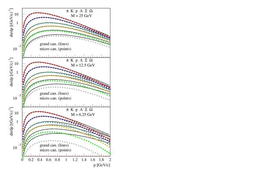
Figure 13: Same as Fig. 12, but for masses $M=25$ GeV, $M=12.5$ GeV, and $M=6.25$ GeV.

Having a reliable method for very large $n$ is in particular useful in order to investigate the convergence towards the infinite volume limit. I will first – also as a check that the procedures work – compare our microcanonical results with grand-canonical decay, knowing that the latter is the limit of the former for large droplets. I consider a “complete” set of hadrons, compatible with a recent PDG (particle data group) list. I consider the decay of droplets of different invariant masses $M$ (corresponding to the total energy $E$ in the above formulas). The volume is chosen such that one has always the same energy density, namely $M/V=\varepsilon_{\mathrm{FO}}=0.57\,\mathrm{GeV}/\mathrm{fm}{}^{3}$, which corresponds to a temperature of $T=167\,$MeV.

In Figs. 12 and 13, I show momentum distributions of pions (red), kaons (blue), protons (green), lambdas (yellow), $\Xi$ baryons (light geen), and $\Omega$ baryons (grey), where one counts particles and antiparticles. I show results for different masses $M$, namely $M=200$ GeV, $M=100$ GeV, $M=50$ GeV, $M=25$ GeV, $M=12.5$ GeV, and $M=6.25$ GeV. I show results for microcanonical particle production (points) compared with the grand canonical one (lines). The grand canonical results are all taken for the same volume, namely $V_{0}=M_{0}/\varepsilon_{\mathrm{FO}}$, with $M_{0}=50$ GeV, to have always the same reference curve, therefore one multiplies the microcanonical results with $M_{0}/M$, to have the correct normalization.

Looking at the $M=200\mathrm{\,GeV}$ results (upper plot in Fig. 12), one sees no difference between the microcanonical and the grand canonical results, which means that this system ( $M=200\mathrm{\,GeV}$ and $V=M/\varepsilon_{\mathrm{FO}}$,) correspond already to the “infinite volume limit”. Considering $M=100\mathrm{\,GeV}$ and $M=50\mathrm{\,GeV}$ (middle and lower plot in Fig. 12), one sees slight deviations of the microcanonical curves from the grand canonical ones, for heavy particles ($\Xi$ baryons and $\Omega$ baryons) and at large $p_{t}$. For pions and kaons, the two scenarios are still identical.

Looking at the plots in Fig. 13, representing $M=25\mathrm{\,GeV}$, $M=12.5\mathrm{\,GeV}$, and $M=6.25\mathrm{\,GeV}$, one sees increasing differences between microcanonical and the grand canonical results, the biggest ones for heavy particles, in particular the $\Omega$ baryons. Finally not only the shape of the distributions is affected, but even the absolute yield. In case of $M=6.25\mathrm{\,GeV}$, one observes a strong $\Omega$ baryon suppression in the microcanonical compared with the grand canonical case.

So far one considers the decay of a static plasma droplet of given mass $M$ and volume $V$ (with $M/V=\varepsilon_{\mathrm{FO}}$), according to the microcanonical probability distribution, whereas in reality, one has an expanding fluid, where fluid cells pass eventually below the critical energy density $\varepsilon_{\mathrm{FO}}$. I discuss in the following how to treat such a case.

IV.3 Flow through hypersurface elements

Let me assume that one has an expanding fluid, characterized by an energy-momentum tensor $T^{\mu\nu}$ and some vector $J_{A}^{\mu}$ representing the current of conserved quantities $A$ (charge, baryon number, strangeness). The energy-momentum tensor can be expanded in the case of a viscous fluid in terms of the energy density $\varepsilon$, the flow vector $u^{\mu}$ (four-velocity of fluid cell), the shear stress tensor, and bulk pressure. Given the space-time dependence of the energy density, one may define a “freeze-out (FO) hypersurface” via

$$\varepsilon(\tau,\eta,r,\varphi)=\varepsilon_{\mathrm{FO}},$$ (29)

such that a point on the FO hypersurface can be expressed as $x^{\mu}(\tau,\eta,r,\varphi)$ with

$$x^{0}=\tau\cosh\eta,\>x^{1}=r\cos\varphi,\>x^{2}=r\sin\varphi,\>x^{3}=\tau\sinh\eta,$$ (30)

with for example $r=r(\tau,\eta,\varphi)$. A hypersurface element [sketched in Fig. 14(a)] may then be defined as

$$d\Sigma_{\mu}=\varepsilon_{\mu\nu\kappa\lambda}\frac{\partial x^{\nu}}{\partial\tau}\frac{\partial x^{\kappa}}{\partial\varphi}\frac{\partial x^{\lambda}}{\partial\eta}\,d\tau\,d\varphi\,d\eta.$$ (31)

One uses Milne coordinates and the corresponding natural frame (see appendix D) for all vector and tensor representations.

Cooper-Frye hadronization amounts to calculating the production of particles with four-momenta $p^{\mu}$ according to

$$E\frac{dn}{d^{3}p}=\int d\Sigma_{\mu}p^{\mu}f_{T}(u^{\nu}p_{\nu}),$$ (32)

with $f_{T}(E)$ being “thermal” (grand canonical) distribution at a given temperature. As sketched in Fig. 14(b),

(a)                        (b)            
            
(c)            
            

Figure 14: (a) FO hypersurface element. (b) Cooper-Frye hadronization as particle flow through FO hypersurface element. (c) The flow of energy-momentum $dP^{\mu}$ through the surface element $d\Sigma_{\mu}$.

the Cooper-Frye procedure amounts to considering particle flow through FO hypersurface elements. Here one is going to proceed differently. Rather than considering particle flow, one considers energy-momentum flow. As sketched in Fig. 14(c), one defines the flow of energy-momentum $dP$ and the flow of conserved charges $dQ_{A}$ through the surface element $d\Sigma$ as

$$dP^{\mu} \boldsymbol{=} T^{\mu\nu}d\Sigma_{\nu},$$ (33)

$$dQ_{A} \boldsymbol{=} J_{A}^{\nu}d\Sigma_{\nu},$$ (34)

with $A\in\{C,B,S\}$, corresponding electric charge, baryon number and strangeness. Momentum and charges are conserved, i.e., $\int_{\Sigma}dP^{\mu}=0$ and $\int_{\Sigma}dQ_{A}=0$ for a closed surface $\Sigma$, and as a consequence, if one starts at some given proper time $\tau_{\mathrm{ini}}$, one gets

$$\int_{\Sigma_{\mathrm{FO}}}dP^{\mu} \boldsymbol{=} P_{\mathrm{ini}}^{\mu},$$ (35)

$$\int_{\Sigma_{\mathrm{FO}}}dQ_{A} \boldsymbol{=} Q_{A\,\mathrm{ini}},$$ (36)

provided the hypersurface $\Sigma_{\mathrm{ini}}$ corresponding to $t_{\mathrm{ini}}$ plus the FO hypersurface $\Sigma_{\mathrm{FO}}$ represent a closed hypersurface, as sketched in Fig. 15.

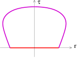
Figure 15: Closed hypersurface $\Sigma_{\mathrm{ini}}$ (red) plus $\Sigma_{\mathrm{FO}}$ (magenta).

This means, when integrating $dP^{\mu}$ and $dQ_{A}$ over the complete FO hypersurface, one recovers completely the initial energy-momentum and conserved charges, and one therefore considers $dP^{\mu}$ and $dQ_{A}$ as the “basic objects” which allow one to realize particle production by respecting the conservation of energy-momentum and of conserved charges.

In practice, one discretizes the hypersurface, and consider small (but finite) elements $\Delta\Sigma^{(K)}$ which cover the whole hypersurface $\Sigma_{\mathrm{FO}}$, as sketched in Fig. 16,

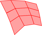
Figure 16: Small hypersurface elements $\Delta\Sigma^{(K)}$ covering the whole hypersurface $\Sigma_{\mathrm{FO}}$.

to be explained in the following. Before defining hypersurface and hypersurface elements, the hydrodynamic evolution is completed, and all relevant quantities (energy density, flow velocity, current of conserved charges, …) are known on a four-dimensional grid $(\tau_{i},\eta_{j},r_{k},\varphi_{n})$, with constant step sizes $\Delta a=a_{i+1}-a_{i}$ for the four variables $a\in\{\tau,\eta,r,\varphi\}$.

The ranges for $r$ and $\eta$ are adapted to the system size (PbPb is obviously bigger than pp) and the energy (for LHC one needs larger $\eta$ ranges than for RHIC energies). First the transverse size $R$ is determined (based on the core distribution in space), event-by-event, such that the freeze-out surface will be covered, with $R$ from 3 fm (peripheral) to 10 fm (central) for PbPb at 2.76 TeV, and with $R=2.4$ for pp at 7 TeV. Then a longitudinal width (in space-time rapidity) $W$ is determined, as $21.2\,r(s)$, with $r(s)=y(s)/y(s_{\mathrm{ref}})$, where $y(s)$ is the rapidity of the projectile nucleons in the nucleon-nucleon center-of-mass for a squared nucleon-nucleon energy $s$, and where $s_{\mathrm{ref}}=(2.76\mathrm{TeV)^{2}}$ is some reference value. Then one defines: $\Delta r=R/74$, $c\Delta\tau=2R/50$, $\Delta\eta=W/26$, $\Delta\varphi=2\pi/60$ (EPOS4.0.0 default).

The hypersurface defined by $\varepsilon(\tau,\eta,r,\varphi)=\varepsilon_{\mathrm{FO}}$ is computed based on the knowledge of the energy density on the grid and is given in terms of four-vectors $x=x^{(i,j,n)}$ depending on three indices $i$, $j$, $n$ as

$$x^{0}=\tau_{i}\cosh\eta_{j},\>x^{1}=r_{i,j,n}\cos\varphi_{n},$$ (37)

$$x^{2}=r_{i,j,n}\sin\varphi_{n},\>x^{3}=\tau_{i}\sinh\eta_{j},$$ (38)

with $r_{i,j,n}$ being the root of $f(r)=\varepsilon(\tau_{i},\eta_{j},r,\varphi_{n})-\varepsilon_{\mathrm{FO}}$, for fixed $i$, $j$, $n$ computed via linear interpolation from the known values of $f(r_{k})$ and $f(r_{k+1})$, where $k$ has been determined such that $f(r_{k})$ and $f(r_{k+1})$ have opposite sign (and $[r_{k},r_{k+1}]$ contains the root). Knowing the hypersurface given as $x=x^{(i,j,n)}$, one defines hypersurface elements $\Delta\Sigma^{(i,j,n)}$ as

$$\Delta\Sigma_{\mu}^{(i,j,n)}=\varepsilon_{\mu\nu\kappa\lambda}\left\{\frac{\partial x^{\nu}}{\partial\tau}\frac{\partial x^{\kappa}}{\partial\varphi}\frac{\partial x^{\lambda}}{\partial\eta}\right\}_{x=x^{(ijn)}}\,\Delta\tau\,\Delta\varphi\,\Delta\eta,$$ (39)

where the partial derivatives are obtained from Eq. (30) and $\Delta\tau$, $\Delta\varphi$, and $\Delta\eta$ are the step sizes of our grid. Having determined $r_{i,j,n}$ via interpolation, one employs the same interpolation procedure to construct the energy-momentum tensor $T^{\mu\nu}$and the current of conserved charges $J_{A}^{\nu}$ corresponding to $r_{i,j,n}$, from the known values of these quantities at grid points $(\tau_{i},\eta_{j},r_{k},\varphi_{n})$ and $(\tau_{i},\eta_{j},r_{k+1},\varphi_{n})$ and use then for the interpolated values the symbols $T^{(i,j,n)\,\mu\nu}$ and $J_{A}^{(i,j,n)\,\nu}$. To simplify the following discussion, one introduces an integer $K=K(i,j,n)$, being uniquely related to the triplet $(i,j,n)$, so one uses the quantities $\Delta\Sigma_{\mu}^{(K)}$, $T^{(K)\,\mu\nu}$ and $J_{A}^{(K)\,\nu}$. One then computes the energy-momentum flow vector $\Delta P^{(K)\,\mu}=T^{(K)\,\mu\nu}\Delta\Sigma_{\nu}^{(K)}$ and the flow of conserved charges $\Delta Q_{A}^{(K)}=J_{A}^{(K)\,\nu}\Delta\Sigma_{\nu}^{(K)}$.

For each hypersurface element $\Delta\Sigma^{(K)}$ and its associated flow vector $\Delta P^{(K)}$, one defines an invariant mass element

$$\Delta M^{(K)}=\sqrt{\Delta P^{(K)}\cdot\Delta P^{(K)}},$$ (40)

where “$\cdot$” refers to a product of four-vectors. One also defines an associated flow four-velocity $U$ as

$$U^{(K)}=\Delta P^{(K)}/\Delta M^{(K)}.$$ (41)

The four-velocity $U^{\boldsymbol{\mu}}$ is NOT equal to the fluid velocity $u^{\mu}$, this would only be true in case of zero pressure.

If one was only interested in global particle yields, one might sum up all the masses to get the total effective invariant mass:

$$M_{\mathrm{eff}}=\sum_{K=1}^{K_{\mathrm{max}}}\Delta M^{(K)},$$ (42)

sum up the charges as

$$Q_{\mathrm{eff}\,A}=\sum_{K=1}^{K_{\mathrm{max}}}\Delta Q_{A}^{(K)},$$ (43)

and decay this object according to microcanonical hadronization, as discussed in the previous section. But in that case, one has no information transverse momentum and rapidity dependencies of particle production.

But one can do better. One still computes $M_{\mathrm{eff}}$ and performs the microcanonical decay, as discussed above. But one actually has much more information than just the masses. One knows in addition for each hypersurface element $\Delta\Sigma^{(K)}$ the associated four-velocity $U^{(K)}$, representing the energy-momentum flow through the surface element, and one knows all its coordinates, see Fig. 17.

Figure 17: For all hypersurface elements (their centers, black points), the coordinates $(\tau,\eta,r,\varphi)$ are known.

Since one counts the hypersurface elements $\Delta\Sigma^{(K)}$ as $K=1,2,3...K_{\mathrm{max}}$, one may define a probability law $P$ on this set $\{1,2,3,...,K_{\mathrm{max}}\}$ as

$$P(K)=\frac{\Delta M^{(K)}}{\sum_{K}\Delta M^{(K)}},$$ (44)

representing the relative weight of a particular hypersurface element. After having done the microcanonical decay, one may consider $P(K)$ as the weight of having produced a particle at a hypersurface position given by the coordinates $\tau_{K},\varphi_{K},r_{K},\eta_{K}$, corresponding to the hypersurface element $\Delta\Sigma^{(K)}$. In other words, one generates the coordinates $\tau_{K},\varphi_{K},r_{K},\eta_{K}$ of the produced hadrons according to the law $P(K)$. In addition, one may consider $P(K)$ also as the weight of having a four-velocity $U^{(K)}$, and so one generates not only the position according to $P(K)$, but also the four-velocity $U^{(K)}$, which one then uses to Lorentz boost the particles into the lab frame (remembering that the microcanonical decay is done in the center-of-mass frame of an effective invariant mass). In other words, one gives back the flow, which has been taken out to construct the effective invariant mass.

In the actual realization of the generation of a set of particles from the Monte Carlo procedure (microcanonical decay plus subsequent sampling based on $P(K)$ and the following boosts of the generated particles according to $U^{(K)}$) one will not have 100% energy-momentum conservation, so one repeats the sampling based on $P(K)$ and the following boosts several times, to take the “best” selection, giving an accuracy on the 1% level.

To test the above procedure, one considers a realistic expanding fluid and the corresponding hypersurface created in a single AuAu simulation at 200 AGeV with an impact parameter of 8 fm, considering a limited $\tau$ range (two steps). Transverse flow velocities on the freeze-out surfacte reach up to 0.45$c$. The total effective mass is around 160 GeV, so this should correspond already to the infinite-volume limit. One therefore computes particle yields in two ways: using the above method of microcanonical decay plus Lorentz boosts according to $U^{(K)}$, based on Monte Carlo simulations, and using the grand canonical method by doing a three-dimensional (3D) momentum integration of Eq. (6), including as well Lorentz boosts according to $U^{(K)}$. The results are shown in Fig. 18,

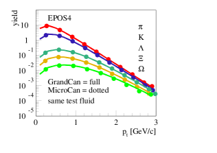
Figure 18: Particle yields in $p_{t}$ bins of width 0.2 GeV/c, computed based on “microcanonical decay + boost” (dotted lines) and based on “grand canonical decay + boost” (full lines), for the same test fluid, see text.

where I plot transverse momentum distributions for different hadron species, from top to bottom: $\pi$, $K$, $\Lambda$, $\Xi$, and $\Omega$ (since one is just interested in comparing two methods, one computes yields in $p_{t}$ bins of width $0.2$ GeV/c, not divided by bin size). As expected, one observes indeed the same result (which is also a good check of the numerics, since the two methods are competely independent of each other).

At very high energies, the above procedure may be problematic, since the FO hypersurface may extend over a wide $\eta$ range, and it is not obvious if it is correct to consider the whole surface as one object with one single effective invariant mass. One therefore has the possibility (and will use it) to split the surface into several pieces corresponding to intervals in $\eta$ with width $\Delta\eta$, as $[\eta_{i}-\Delta\eta/2,\eta_{i}+\Delta\eta/2]$, with $\eta_{i+1}-\eta_{i}=\Delta\eta$. One may then do the sum as in Eq. (42), but just summing the hypersurface elements within $I(\eta_{i})=[\eta_{i}-\Delta\eta/2,\eta_{i}+\Delta\eta/2]$, i.e.

$$\Delta M_{\mathrm{eff}}(\eta_{i})=\sum_{\eta(K)\in I(\eta_{i})}\Delta M^{(K)},$$ (45)

[and correspondingly for $Q_{\mathrm{eff}\,A}(\eta_{i})$] where $\eta(K)$ is the $\eta$ value associated with $K$. Rather than a single effective mass, one has now a discrete set of masses $\Delta M_{\mathrm{eff}}(\eta_{i})$, which one may decay independently in their center-of-mass frames (in the same way as dicussed for $M_{\mathrm{eff}}$. One also notes the rapidities $y_{i}$ corresponding to $\Delta M_{\mathrm{eff}}(\eta_{i})$, which allows one to finally boost the particles into the lab frame. It should be noted that the numerical values of $y_{i}$ are very close to $\eta_{i}$.

One has to do this splitting carefully. If the $\Delta\eta$ interval is chosen to be very small, one may create artificially small masses, with the corresponding suppression of heavy mass hadrons. In this sense, the width $\Delta\eta$ is a physical parameter, measuring the width where hypersurface elements are causally connected. I will come back to this point later.

Let me finally address a technical issue. When constructing objects for given $\eta$ intervals, after summing $\Delta Q_{A}^{(K)}$ elements within this interval, one may end up with non-integer values, which is modified by taking the next-closest integer instead. The violation of the global conservation laws even at RHIC energies is small (less than 1%), so for the moment no correction is applied. This might be changed in the future, but in particular at low energies there are even more important issues to be considered (breakdown of the parallel scattering scheme, first of all). But it is planned to reconsider these issues in a future work dedicated to lower energies.

IV.4 Core hadronization in pp scattering

I will apply the procedures discussed in the last section to investigate proton-proton scattering at LHC energies (I will show results for a center-of-mass energy of 7 TeV), and I will try to understand what kind of effective masses are produced, and where they are produced in space and time.

(a) 2 Pomerons $\tau_{0}$            (b) 2 Pomerons $\tau_{1}$

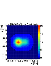
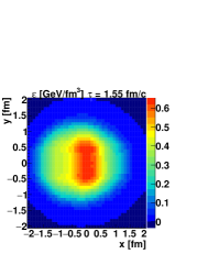
(c) 6 Pomerons $\tau_{0}$            (d) 6 Pomerons $\tau_{1}$

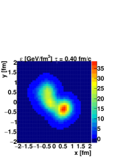
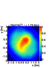
(e) 12 Pomerons $\tau_{0}$            (f) 12 Pomerons $\tau_{1}$

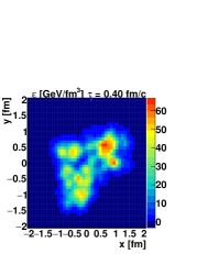
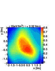
Figure 19: Energy density in the transverse plane ($x,y)$ for proton-proton scattering involving (from top to bottom) 2, 6, and 12 Pomerons. The left column represents the start time $\tau_{0}$ (of the hydro evolution), and the right column a later time $\tau_{1}$, close to final freeze-out.

Let me consider (randomly chosen, but typical) proton-proton scattering events involving 2 Pomerons, 6 Pomerons, and 12 Pomerons. In Fig. 19, I plot for the three cases the energy density in the transverse plane ($x,y)$. I consider in each case two snapshots, namely at the start time of the hydro evolution $\tau_{0}=0.40\,\mathrm{fm/c}$ (left column) and a later time $\tau_{1}$ (different values, $1.5-2.5\,\mathrm{fm/c}$) close to final freeze-out (right column). In all cases, the initial distributions have elongated shapes (just by accident, due to the random positions of interacting partons). One can clearly see that the final distributions are as well elongated, but perpendicular to the initial ones, as expected in a hydrodynamical expansion.

As explained in the last section, one computes effective mass elements representing the momentum flow through surface elements. It is in particular useful to split the $\eta$ range into intervals $[\eta_{i}-\Delta\eta/2,\eta_{i}+\Delta\eta/2]$, with $\eta_{i+1}-\eta_{i}=\Delta\eta$, and sum up the corresponding hypersurface elements to get a set of effective masses $\Delta M_{\mathrm{eff}}(\eta_{i})$. In this way, one obtains an “effective mass distribution” $\Delta M/\Delta\eta$, which one may plot as a function of $\eta$, as shown in Fig. 20 for the above-mentioned events with 2 Pomerons (corresponding roughly to minimum bias), events with 6 Pomerons (roughly 3 times minimum bias), and events with 12 Pomerons, (roughly 6 times minimum bias).

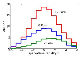
Figure 20: Mass distribution $\Delta M/\Delta\eta$ as a function of the space-time rapidity $\eta$, for an event with 2 Pomerons, an event with 6 Pomerons, and an event with 12 Pomerons.

As expected, the $dM/d\eta$ values increase with increasing Pomeron number, somewhat less than linear.

The total energy (of the core part) may be estimated as

$$E=\sum\frac{\Delta M}{\Delta\eta}(\eta_{i})\,\cosh(\eta_{i})\Delta\eta,$$ (46)

using the fact that $y_{i}$ is very close to $\eta_{i}$. One gets for the three cases:

$$E=\left\{\begin{array}[]{cc}573\,\mathrm{GeV}&\,\,\,(2\,\mathrm{Pom})\\ 1843\,\mathrm{GeV}&\,\,\,(6\,\mathrm{Pom})\\ 2225\,\mathrm{GeV}&\,\,\,(12\,\mathrm{Pom})\end{array}\right.$$ (47)

These numbers should be compared with the total available energy, which is $7000$ GeV. This shows that the total energies of the core part in all three cases represent only a relatively small fraction of the total energy, but the observable effects are big! One may now compute the total effective masses as

$$M_{\mathrm{eff}}=\sum\frac{\Delta M}{\Delta\eta}(\eta_{i})\Delta\eta,$$ (48)

and one gets for the three cases:

$$M_{\mathrm{eff}}=\left\{\begin{array}[]{cc}30.6\,\mathrm{GeV}&\,\,\,(2\,\mathrm{Pom})\\ 61.4\,\mathrm{GeV}&\,\,\,(6\,\mathrm{Pom})\\ 115.4\,\mathrm{GeV}&\,\,\,(12\,\mathrm{Pom})\end{array}\right.$$ (49)

These numbers are much smaller than the energies $E$, the latter ones containing the kinetic energy of the longitudinal expansion. So the masses $M$ are the relevant quantities concerning the production yields for the different particle species, and these masses will be used in the micro-canonical decay procedures.

The effective masses $\Delta M_{\mathrm{eff}}(\eta_{i})$ are sums of small hypersurface elements $\Delta\Sigma^{(K)}$, each one corresponding to a set of coordinates $\tau,\eta,r,\varphi$, which allows one to plot projections of these coordinates into the $\eta-\tau$ plane, as done

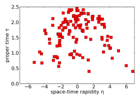
Figure 21: Hypersurface element positions projected into the $\eta-\tau$ plane.

in Fig. 21 for our 12-Pomeron example. This shows that the hypersurface is quite extended in space and time. In general, hadronization at large space-time rapidities (corresponding to large rapidities) happens early, the latest hadronization takes place around $\eta=0$, the extension in time is around 2 fm/c, the width in $\eta$ is around 10 units.

In particular the important width in $\eta$ brings up (again) the question of how to deal with the splitting of the complete hypersurface into pieces of width $\Delta\eta$, as sketched in Fig. 22.

Figure 22: Splitting of the complete hypersurface (left) into pieces of width $\Delta\eta$ (right).

For small systems (like pp scattering), the total effective masses are not very big, in our three examples between 30 and 115 GeV, and splitting these into small pieces will lead to very small effective masses, with big effects concerning the production of heavy baryons. As shown in Sec. IV.2, for masses at 25 GeV, one sees already deviations in the microcanonical result compared with the grand canonical one. So the big question is: does the system decay as single effective mass $M_{\mathrm{eff}}$ or as several independent objects of width $\Delta\eta$.

in Refs. [31, 32], Oliinychenko et al. presented a sampling method for the transition from relativistic hydrodynamics to particle transport, which preserves the local event-by-event conservation of energy, momentum, baryon number, strangeness, and electric charge, for each sampled configuration in spatially compact regions (patches). In our method, using finite $\Delta\eta$ amounts to cutting the hypersurface into distinct regions, defined by $\eta$ ranges. In principle it would be possible to further cut these regions into smaller pieces, which indeed might be necessary to study local fluctuations. This is an option for future development, but I do not follow this possibility in this paper, since I mainly focus on the transition to small systems, where already the regions defined by $\eta$ ranges are small.

IV.5 The role of the splitting parameter $\boldsymbol{\boldsymbol{\Delta\eta}}$ in core hadronization

Let me consider $\Delta\eta$ as a free parameter, in order to try several choices of $\Delta\eta$ in the following, to learn how it affects the results. One choice will be $\Delta\eta=\infty$, which means one has just one single object as in Fig. 22 (left). In addition, one also investigates $\Delta\eta=4.5$ and $\Delta\eta=1.8$, as in Fig. 22 (right).

One should keep in mind that the total width of the FO hypersurface is around 10 fm/c, at LHC energies, see Fig. 21, and the total effective masses in pp scattering are between several tens up to more than 100 GeV, depending on the Pomeron number.

One considers only the core contributions for the moment, decayed according to microcanonical hadronization, for pp and PbPb scattering. Particle ratios (with respect to pions always) are computed as a function of the charged multiplicity $\left\langle dn_{\mathrm{ch}}/d\eta(0)\right\rangle$, which allows one to put pp and PbPb results on the same plot. One considers simulation results from EPOS4.0.0 for pp at 7 TeV and PbPb at 2.76 TeV, compared with data from ALICE [33, 34, 6, 35, 7]. In Fig. 23, I show

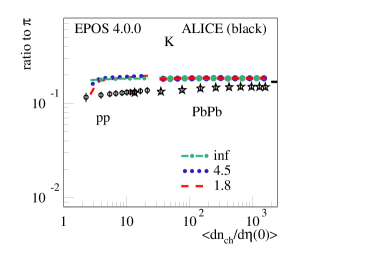
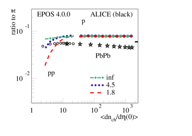
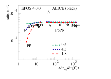
Figure 23: Ratio $K/\pi$ (upper plot), $p/\pi$ (middle plot), and $\Lambda/\pi$ (lower plot), for pp at 7 TeV and PbPb at 2.76 TeV as a function of the multiplicity $dn_{\mathrm{ch}}/d\eta(\eta=0)$, compared with ALICE data.

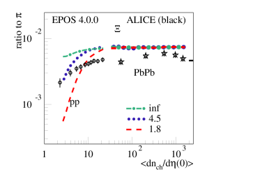
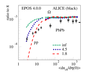
Figure 24: Same as Fig. 23, but for $\Xi/\pi$ (upper plot) and $\Omega/\pi$ (lower plot).

results for $K/\pi$ (upper plot), $p/\pi$ (middle plot), and $\Lambda/\pi$ (lower plot), and in Fig. 24 results for $\Xi/\pi$ (upper plot) and $\Omega/\pi$ (lower plot). In all cases, I show simulation results for $\Delta\eta=\infty$ (green dashed-dotted lines), $\Delta\eta=4.5$ (blue dotted lines) and $\Delta\eta=1.8$ (red dahsed lines). For the simulation results, thin line style is used for pp, and thick lines for PbPb, whereas for the data, circles are used for pp and stars for PbPb. The short black horizontal lines on the right side of the plots correspond to predictions from the “thermal model” [36].

First of all, one sees that all the curves show a continuous behavior, when passing from pp to PbPb. Concerning the PbPb results, there is no difference between the the three $\Delta\eta$ choices, with the only exception of $\Omega/\pi$ ratios, where the $\Delta\eta=\infty$ gives a flat ratio, whereas for $\Delta\eta=4.5$ and $\Delta\eta=1.8$ the curves drop slightly on the left end (peripheral collisions). The situation is quite different for the pp curves. In all cases, the curves drop when going to smaller multiplicities, and this drop is more and more pronounced with decreasing $\Delta\eta$, and comparing the curves with fixed $\Delta\eta$, the drop is increasing with particle mass: the biggest effect is seen for $\Omega/\pi$ ratios. One should also keep in mind that grand canonical particle production (what has been used in earlier EPOS version) leads to flat curves, the same for pp and PbPb. So one sees a big effect of microcanonical hadronization compared to the grand canonical one, and the deviation depends strongly on $\Delta\eta$.

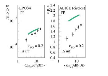
Figure 25: Ratio $\Omega/\pi$ (left plot) and average $p_{t}$ (right plot) for pp at 7 TeV, for $\Delta\eta=\infty$ and $\varepsilon_{\mathrm{FO}}=0.2$. EPOS simulations are compared with data from ALICE [7].

Concerning the comparison with experimental data, one sees that none of the choices of $\Delta\eta$ can explain the data: for big values of $\Delta\eta$, one stays clearly above the data, and for small values, the ratios do drop sufficiently, but too fast. So it is clear that even a “tuning” of $\Delta\eta$ will not help to reproduce the data – for a pure core approach. I will investigate the full core-corona approach in the next section.

As a side remark: it is of course possible to reduce baryon production by using a smaller value of the freeze-out energy density $\varepsilon_{\mathrm{FO}}$, as shown in Fig. 25 (left), where I plot the ratio $\Omega/\pi$ for a pp simulation at 7 TeV, using $\Delta\eta=\infty$ and $\varepsilon_{\mathrm{FO}}=0.2$. But as seen in 25 (right), the average $p_{t}$ is much too high. Similar results are obtained for other baryons. So it seems impossible to reproduce in this way ratios and other important observables at the same time, as it will be possble in the core-corona approach, where in addition, one employs a unique value of $\varepsilon_{\mathrm{FO}}$ for all systems.

IV.6 Results for the full core-corona picture in pp and PbPb scattering

In the following, results concerning the full core-corona approach will be discussed. Let me briefly recall the procedure: as explained in detail in Sec. III, primary interactions lead to the production of prehadrons, a core-corona procedure separates the core and corona prehadrons. The former constitute the core, the latter are considered to be hadrons. The core is meant to be matter, which evolves according to viscous hydrodynamics, which allows one to compute the space-time dependence of the energy-momentum tensor $T^{\mu\nu}$ (expressed in terms of energy density $\varepsilon$, the flow vector $u^{\mu}$, the shear stress tensor, and bulk pressure) and of the vector $J_{A}^{\mu}$ representing the current of conserved quantities $A$.

As shown in Sec. IV.3, based on the energy density $\varepsilon$, one defines a freeze-out (FO) hypersurface via $\varepsilon(\tau,\eta,r,\varphi)=\varepsilon_{\mathrm{FO}}$, which allows defining (after discretization) small hypersurface elements $\Delta\Sigma_{\mu}$. Together with the knowledge of $T^{\mu\nu}$, this allows one to compute energy-momentum flow four-vectors $\Delta P$ and invariant mass elements $\Delta M=\sqrt{\Delta P\cdot\Delta P}$, which may be summed up to get effective invariant masses $\Delta M_{\mathrm{eff}}(\eta_{i})$, covering space-time rapidity intervals of width $\Delta\eta$, which are decayed microcanonically (this is called “hadronization”).

As discussed in the previous section, the outcome of core hadronization depends on $\Delta\eta$. I use in the following $\Delta\eta=\infty$, which seems to be “the best” value when comparing with data, in the sense of a comparison with very large set of data concerning very different observables, for many different systems and energies, much beyond what is shown in this paper. The aim of this work is not to accommodate local fluctuations, in that case one needed in particular for heavy ion collisions to introduce “local patches” and not only finite $\Delta\eta$, which would be an easy extension of the present work. The main focus here is the transition from big to small systems, and for small systems the value of $\Delta\eta$ is important, and (from our findings) the best global fit is obtained for $\Delta\eta=\infty$, which is simply an empirical fact, somewhat counterintuitive. Anyway, $\Delta\eta$ is one of the EPOS parameters the user may change.

After the hadronization of the fluid, the created hadrons as well as the corona prehadrons (having been promoted to hadrons) may still interact via hadronic scatterings, and here one uses UrQMD [37, 38].

In the following, I want to study core and corona contributions to hadrons production, for pp and PbPb collisons at LHC energies. I will distinguish:

(A)

The “core+corona” contribution: primary interactions (S-matrix approach for parallel scatterings), plus core-corona separation, hydrodynamic evolution, and microcanonical hadronization, but without hadronic rescattering.

(B)

The “core” contribution: like (A), but considering only core particles.

(C)

The “corona” contribution: like (A), but considering only corona particles.

(D)

The “full” EPOS4 scheme: like (A), but in addition hadronic rescattering.

In cases (A), (B), and (C), one needs to exclude the hadronic afterburner, because the latter affects both core and corona particles, so in the full approach, the core and corona contributions are not visible anymore.

In Fig. 26,

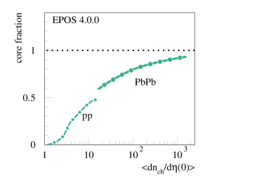
Figure 26: The core fraction [core / (core+corona)] for pp at 7 TeV and PbPb at 2.76 TeV as a function of the multiplicity $dn_{\mathrm{ch}}/d\eta(\eta=0)$.

I show the core fraction [core / (core+corona)] in pp at 7 TeV and PbPb at 2.76 TeV as a function of the multiplicity $dn_{\mathrm{ch}}/d\eta(\eta=0)$, being defined as pion yield from core over core + corona contribution (since pions are by far the most frequent species).

I will take core+corona as a reference, and plot ratios X / core+corona versus $p_{t}$, with X being the corona contribution, the core , and the full contribution, for four event classes and four different particle species.

In Fig. 27, I show results for pp collisions at 7 TeV, for (from top to bottom) pions ($\pi^{\pm}$), kaons ($K^{\pm}$), protons ($p$ and $\bar{p}$), and lambdas ($\Lambda$ and $\bar{\Lambda}$), which correspond to hadrons with increasing masses.

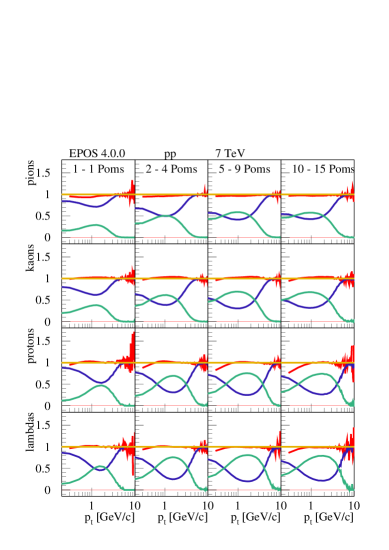
Figure 27: The X / core+corona ratio, with X being the corona contribution (blue), the core (green), and the full contribution (red), for four event classes and four different particle species, for pp at 7 TeV.

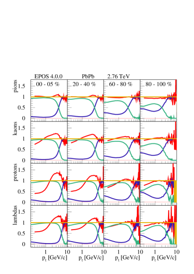
Figure 28: The X / core+corona ratio, with X being the corona contribution (blue), the core (green), and the full contribution (red), for four centrality classes and four different particle species, for PbPb at 2.76 TeV.

The four columns represent four different event classes defined in terms of the number $N_{\mathrm{Pom}}$ of Pomerons (from left to right): 1, 2-4, 5-9, 10-15, which may be compared with the average number of Pomerons in minimum bias pp at 7 TeV of around 2.

Looking at the green (core) and blue (corona) curves, one observes that the core contribution increases with $N_{\mathrm{Pom}}$, but it also increases with the hadron mass (from top to bottom). The biggest core contribution is observed for lambdas for events with 10-15 Pomerons. There is an interesting $p_{t}$ dependence. In all cases, the maximum of the green core curves is around 1-2$\,\mathrm{GeV/c}$, with bigger values for the heavier particles. This is clearly a flow effect, the core particles are produced from a radially expanding fluid, which moves particles to higher $p_{t}$ values, as compared with a decaying static droplet.

Whereas the core contribution goes down toward small $N_{\mathrm{Pom}}$, one still observes a non-vanishing contribution even for $N_{\mathrm{Pom}}=1$, which means even a very small number of strings may create a core and flow effects. And this is actually needed to describe experimental data, as I discuss later. It is often said that “collective effects” show up in high multiplicity pp events, but it seems that flow effects are present everywhere.

The red curves represent full over core+corona, the difference between the two is the effect of the hadronic cascade in the full case. Here, one sees only a small effect, essentially some baryon-antibaryon annihilation, which suppresses the baryon yield at small $p_{t}$.

In Fig. 28, I show ratios X / core+corona versus $p_{t}$, for PbPb collisions at 2.76 TeV, again for (from top to bottom) pions ($\pi^{\pm}$), kaons ($K^{\pm}$), protons ($p$ and $\bar{p}$), and lambdas ($\Lambda$ and $\bar{\Lambda}$). The four columns represent four different centrality classes, namely 0-5%, 20-40%, 60-80%, 80-100%.

Looking at the green (core) and blue (corona) curves, one observes that the core contribution increases with centrality, but it also increases with the hadron mass (from top to bottom). Concerning the $p_{t}$ dependence, one also observes a maximum of the green core curves around 1-2$\,\mathrm{GeV/c}$, less pronounced compared with the pp results, but still, at very low $p_{t}$ the core contribution goes down, so even at very small $p_{t}$ values the corona contributes. The crossing of the green core and the blue corona curves (core = corona) occurs between around 2GeV/c (mesons, peripheral) and 5GeV/c (baryons, central).

The red curve, full over core+corona, represents the effect of the hadronic cascade in the full case. The pions are not much affected, but for kaons and even more for protons and lambdas, rescattering makes the spectra harder. One should keep in mind that rescattering involves particles from fluid hadronization, but also corona particles from hard processes. Concerning the baryons, rescattering reduces (considerably) low $p_{t}$ yields, due to baryon-antibaryon annihilation.

In the following, I show results of particle production in pp scattering at 7 TeV and PbPb collisions at 2.76 TeV.

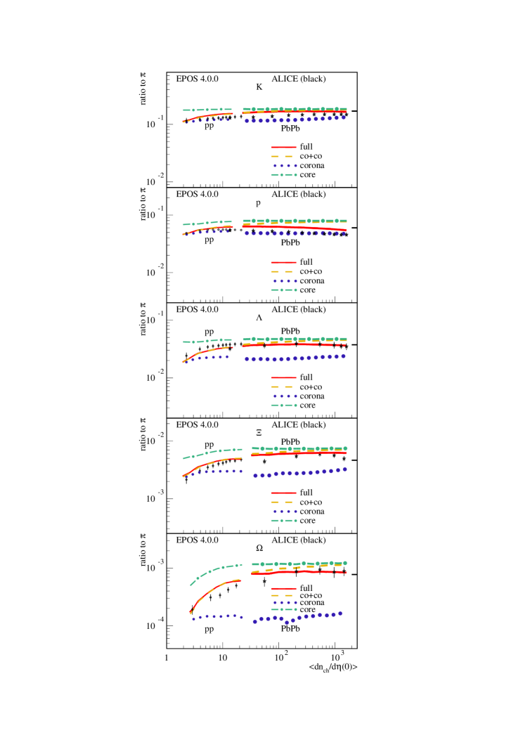
Figure 29: Ratio to $\pi$ for (from top to bottom) $K$, $p$, $\Lambda$, $\Xi$, $\Omega$ for pp at 7 TeV and PbPb at 2.76 TeV as a function of the multiplicity $dn_{\mathrm{ch}}/d\eta(\eta=0)$. I show the different contributions: core, corona, core+corona, and full (see text), compared with ALICE data.

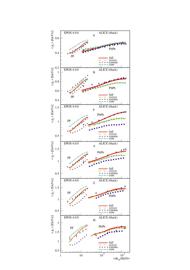
Figure 30: Average transverse momentum of (from top to bottom) $\pi$, $K$, $p$, $\Lambda$, $\Xi$, $\Omega$ for pp at 7 TeV and PbPb at 2.76 TeV as a function of the multiplicity $dn_{\mathrm{ch}}/d\eta(\eta=0)$. I show the different contributions: core, corona, core+corona, and full (see text), compared with ALICE data.

In Fig. 29, I show ratios of hadron yields over pion yields, at rapidity zero, for proton-proton scattering at 7 TeV and PbPb at 2.76 TeV, as a function of the average multiplicity $\left\langle dn_{\mathrm{ch}}/d\eta(\eta=0)\right\rangle$. Concerning the EPOS simulations, I show the different contributions: core (green dashed-dotted lines), corona (blue dotted lines), core+corona (co+co, yellow dashed lines), and full (red full lines). Thin lines are used for pp and thick ones for PbPb. I also show ALICE data [33, 34, 6, 35, 7], using black symbols, stars for PbPb, and circles for pp. I consider charged kaons, protons, lambdas, as well as $\Xi$ baryons and $\Omega$ baryons.

One sees almost flat lines for the corona contributions, similar for pp and PbPb, which is understandable, since corona means particle production from string fragmentation, which does not depend on the system. One observes also flat curves for the core at high multiplicity, which is again expected since the core hadronization is determined by the freeze-out energy density, which is system independent. However, when the system gets very small, one gets a reduction of heavy particle production due to the microcanonical procedure (with its energy and flavor conservation constraints), whereas a grand canonical treatment would give a flat curve down to small multiplicities. This effect increases with particle mass, it is biggest for Omega baryons, where the reduction is about a factor of 2.

The yellow core+corona curves simply interpolate between the corona and the core curves, with the core weight increasing continuously with multiplicity. The increase is biggest for the $\Omega$. Here, the core curve is far above the corona one, which simply reflects the fact that $\Omega$ production is much more suppressed in string decay, compared with statistical (“thermal”) production. This explains why the core+corona contribution increases by one order of magnitude from low to high multiplicity, because simply the relative weight of the core fraction increases from zero to unity. Both microcanonical decay and core-corona procedure contribute to the decrease of the ratios toward small multiplicity, but it seems that the core-corona mechanism is more important.

Finally, there is some effect from hadronic rescattering (difference between full and co+co), mainly a suppression due to baryon-antibaryon annihilation at large multiplicities.

Whereas the particle ratios are essentially smooth curves, from pp to PbPb, the situation changes completely when looking at the average transverse momentum $\left\langle p_{t}\right\rangle$ versus multiplicity, as shown in Fig. 30, where I show simulation results for pp (thin curves) and PbPb (thick curves) for charged $\pi$ mesons, charged $K$ mesons, (anti)protons, $\Lambda$ (anti)baryons, $\Xi$ (anti)baryons, and $\Omega$ (anti)baryons. I again show the different contributions: core (green dashed-dotted lines), corona (blue dotted lines), core+corona (co+co, yellow dashed lines), and full (red full lines). Simulation are compared with ALICE data [33, 34, 6, 35, 7], using black symbols, stars for PbPb, and circles for pp.

Here, one sees (for all curves) a significant discontinuity when going from pp to PbPb. The corona contributions are not flat (as the ratios), but they increase with multiplicity, in the case of pp even more pronounced as for PbPb. This is a “saturation effect”: the saturation scale increases with multiplicity, which means that with increasing multiplicity the events get harder, producing higher $p_{t}$. The situation is different for PbPb, where an increase in multiplicity is mainly due to an increase in the number of active nucleons, with a more modest increase of the saturation scale with multiplicity. Also, the core curves increase strongly with multiplicity, and here as well more pronounced in the case of pp, due to the fact that one gets for high-multiplicity pp high energy densities within a small volume, leading to strong radial flow. Again, the core+corona contribution is understood based on the continuous increase of the core fraction from low to high multiplicity.

It is very useful (and necessary) to consider at the same time the multiplicity dependence of particle ratios and of mean $p_{t}$ results, since their behavior is completely different (the former is continuous, the latter jumps). Despite these even qualitative differences between the two observables, the physics issues behind these results is the same, namely saturation, core-corona effects which mix flow (being very strong) and non-flow, and microcanonical hadronization of the core.

Another very important and useful variable is the multiplicity dependence of $D$ meson production, where “D” stands for the sum of $D^{0}$, $D^{+}$, and $D^{*+}$. This is much more than just “another particle”, since the $D$ meson contains a charm quark, the latter being created exclusively in the parton ladder and not during fragmentation or in the plasma. In Fig. 31,

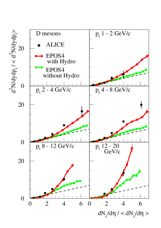
Figure 31: Normalized $D$ meson multiplicity as a function of the normalized charged particle multiplicity for different $p_{t}$ ranges in pp scattering at 7 TeV. I show EPOS results with and without hydro, compared with ALICE data.

I plot the normalized $D$ meson multiplicity ($\frac{d^{2}N}{dydp_{t}}/<\!\!\frac{d^{2}N}{dydp_{t}}\!\!>$) as a function of the normalized charged particle multiplicity ($\frac{dN_{c}}{dy}/<\!\!\frac{dN_{c}}{dy}\!\!>$) for different $p_{t}$ ranges in pp scattering at 7 TeV, compared with ALICE data [39]. It is interesting to see in which way the simulations and the data deviate from the reference curve, which is the dashed black line representing identical multiplicity dependence for D mesons and charged particles. Considering the EPOS results without hydro (green lines), for low $p_{t}$ (1-2 GeV/c) the curve is slightly above the reference, but with increasing $p_{t}$ the green curves get steeper, which is due to the fact that with increasing multiplicity the saturation scale increases, and the events get harder, producing more easily both high-$p_{t}$ and charmed particles. Considering EPOS with hydro (red curves), the increase compared with the green curves is much stronger, which is due to the fact that “turning on hydro” will reduce the multiplicity (the available energy is partly transformed into flow). The red curves are close to the experimental data, both showing a much stronger increase compared with the reference curve, with the effect getting bigger with increasing $p_{t}$. So one may conclude this paragraph: to get these final results (the strong increase), two phenomena are crucial, namely, saturation which makes high multiplicity events harder, and the “hydro effect” which reduces multiplicity and “compresses” the multiplicity axis.

V Summary

After recalling briefly the EPOS4 parallel scattering approach, as well as the core-corona method, I presented new developments concerning the microcanonical decay of plasma droplets, providing very efficient methods to decay droplets of all sizes, allowing the study of the transition towards the grand canonical limit (the method usually employed). I then discussed in detail new methods to construct effective (droplet) masses from energy-momentum flow through freeze-out hypersurfaces of expanding fluids in pp or AA collisions, and I discussed results of microcanonical decay of these droplets. Finally, I investigated the multiplicity dependence of multistrange hadron yields in proton-proton and lead-lead collisions at several TeV, which allows the study of the transition from very big to very small systems, in particular concerning collective effects. Here, the “full model” was employed: our core-corona approach, using new microcanonical hadronization procedures, as well as the new methods allowing to transform energy-momentum flow through freeze-out surfaces into invariant-mass elements. It was tried to disentangle effects due to “canonical suppression” and “core-corona effects”, which will both lead to a reduction of the yields at low multiplicity.

APPENDIX

Appendix A The NRPS integral

The NRPS integral Eq. (14) may be written as (writing $\Phi$ instead of $\Phi_{\mathrm{NRPS}}$)

$$\Phi =(4\pi)^{n}\int_{m_{1}}^{\infty}dE_{1}\ldots\int_{m_{n}}^{\infty}dE_{n}\prod_{i=1}^{n}p_{i}\,E_{i}$$ (50)

$$\times\delta(M-\sum_{i=1}^{n}E_{i})\,W(p_{1},\ldots,p_{n}).$$ (51)

With $t_{i}:=E_{i}-m_{i}$ and $T:=M-\sum_{i=1}^{n}m_{i}$ one obtains

$$\Phi(M,m_{1},\ldots,m_{n}) = (4\pi)^{n}\int_{0}^{\infty}dt_{1}\ldots\int_{0}^{\infty}dt_{n}\prod_{i=1}^{n}p_{i}\,\varepsilon_{i}$$ (52)

$$\times\,\delta\big{(}T-\sum_{i=1}^{n}t_{i}\big{)}\,W(p_{1},\ldots,p_{n}).$$

One now introduces “accumulated” kinetic energies $s_{i}$ via

$$s_{i}:=\sum_{j=1}^{i}t_{j},$$ (53)

with the inverse $t_{i}=s_{i}-s_{i-1},\quad s_{0}=0$ and $dt_{i}=ds_{i}$. One obtains

$$\Phi(M,m_{1},\ldots,m_{n})=(4\pi)^{n}\int_{0}^{\infty}ds_{1}\int_{s_{1}}^{\infty}ds_{2}\ldots\int_{s_{n-1}}^{\infty}ds_{n}$$

$$\quad\quad\quad\times\prod_{i=1}^{n}p_{i}\,\varepsilon_{i}\,\delta(T-s_{n})W(p_{1},\ldots,p_{n}).$$ (54)

The integration over $s_{n}$ is trivial and may be performed, to obtain

$$\Phi(M,m_{1},\ldots,m_{n})$$

$$\quad\quad\quad=(4\pi)^{n}\int_{0}^{\infty}ds_{1}\int_{s_{1}}^{\infty}ds_{2}\ldots\int_{s_{n-3}}^{\infty}ds_{n-2}\int_{s_{n-2}}^{T}ds_{n-1}$$

$$\quad\quad\quad\times\prod_{i=1}^{n}p_{i}\,\varepsilon_{i}\,W(p_{1},\ldots,p_{n}).$$ (55)

All upper limits may be replaced by $T$. Introducing energy fractions, $x_{i}:=s_{i}/T,$ one gets

$$\Phi(M,m_{1},\ldots,m_{n})=(4\pi)^{n}\,T^{n-1}$$ (56)

$$\times\int_{0\leq x_{1}\leq\ldots\leq x_{n-1}\leq 1}dx_{1}\ldots dx_{n-1}\prod_{i=1}^{n}p_{i}\,\varepsilon_{i}\,W(p_{1},\ldots,p_{n}).$$

Using the definition

$$\psi(p_{1},\ldots,p_{n}):=\frac{(4\pi)^{n}\,T^{n-1}}{(n-1)!}\prod_{i=1}^{n}p_{i}\,\varepsilon_{i}\,W(p_{1},\ldots,p_{n}),$$ (57)

One may write

$$\Phi(M,m_{1},\ldots,m_{n})$$ (58)

$$=(n\!-\!1)!\!\int_{0\leq x_{1}\leq\ldots\leq x_{n-1}\leq 1}dx_{1}\ldots dx_{n-1}\psi(x_{1},\ldots,x_{n-1}),$$

where $\psi(x_{1},\ldots,x_{n-1})$ is meant to be $\psi(p_{1},\ldots,p_{n})$ with $p_{i}$ and $\varepsilon_{i}$ expressed in terms of $x_{1},\ldots,x_{n-1}$. This may be solved via Monte Carlo as

$$\Phi(M,m_{1},\ldots,m_{n})=\frac{1}{N}\sum_{\beta=1}^{N}\psi(x_{1}^{(\beta)}\ldots x_{n-1}^{(\beta)}),$$ (59)

where the $x_{i}^{(\beta)}$ are ordered random numbers,

$$0\leq x_{1}^{(\beta)}\leq x_{2}^{(\beta)}\leq\ldots\leq x_{n-1}^{(\beta)}\leq 1.$$ (60)

So for each Monte Carlo step, $n-1$ random numbers have to be generated, ordered according to size, and then used to evaluate $\psi(x_{1}^{(\beta)},\ldots,x_{n-1}^{(\beta)})$. To avoid ordering, one may introduce the variables

$$z_{i}:=\frac{x_{i}}{x_{i+1}},$$ (61)

using the definition $x_{n}:=1$. One gets

$$dx_{i}=dz_{i}\,x_{i+1}=dz_{i}\prod_{j=i+1}^{n-1}z_{j},$$ (62)

the last equation holding for $i<n-1$; so one has

$$\prod_{i=1}^{n-1}dx_{i} = \prod_{i=1}^{n-1}dz_{i}\prod_{i=1}^{n-2}\prod_{j=i+1}^{n-1}z_{j}$$ (63)

$$= \prod_{i=1}^{n-1}dz_{i}\prod_{i=1}^{n-1}z_{i}^{i-1}.$$

From Eq. (58), one gets

$$\Phi(M,m_{1},\ldots,m_{n})$$ (64)

$$=\int_{0}^{1}dz_{1}\ldots\int_{0}^{1}dz_{n-1}\prod_{i=1}^{n-1}i\,z_{i}^{i-1}\,\psi(z_{1},\ldots,z_{n-1}),$$

where obviously $\psi(z_{1},\ldots,z_{n-1})$ is meant to be $\psi(p_{1},\ldots,p_{n})$ with $p_{i}$ expressed in terms of $z_{i}$. One now introduces

$$r_{i}:=\int_{0}^{z_{i}}i\,\xi^{i-1}\,d\xi=z_{i}^{i}$$ (65)

to obtain

$$\Phi(M,m_{1},\ldots,m_{n})=\int_{0}^{1}dr_{1}\ldots\int_{0}^{1}dr_{n-1}\,\psi(r_{1},\ldots,r_{n-1}).$$ (66)

The $r_{i}$ are now uncorrelated, no ordering is required. The final result is $\Phi=\int d\Phi$ with

$$d\Phi=dr_{1}...dr_{n-1}\frac{(4\pi)^{n}\,T^{n-1}}{(n-1)!}\prod_{i=1}^{n}p_{i}\,E_{i}\,W(p_{1},...,p_{n}),$$ (67)

with $r_{i}\in[0,1]$, and with $z_{i}=r_{i}^{1/i}$,  $x_{i}=z_{i}x_{i+1}$,  $s_{i}=x_{i}T$,  $t_{i}=s_{i}-s_{i-1}$,  $E_{i}=t_{i}+m_{i}$,  $T=M-\sum_{i=1}^{n}m_{i}$.

Appendix B The LIPS integral

For given mass $M$, for given $n$, and for given masses $m_{1},...,m_{n}$, one defines the LIPS phase-space integral $\Phi_{\mathrm{LIPS}}=\int d\Phi_{\mathrm{LIPS}}$ as

$$\Phi_{\mathrm{LIPS}}=\int\delta(M-\Sigma E_{i})\,\delta^{3}(\Sigma\vec{p}_{i})\,\prod_{i=1}^{n}\frac{d^{3}p_{i}}{\,2E_{i}},$$ (68)

which may be written as [28]

$$\Phi_{\mathrm{LIPS}}=\int\delta^{4}(P-\Sigma p_{i})\,\prod_{i=1}^{n}\delta(p_{i}^{2}-m_{i}^{2})d^{4}p_{i}\qquad\qquad\qquad$$ (69)

$$\quad=\int\left\{\int\delta^{4}\left(P\!-\!P_{l}\!-\!\sum_{i>l}p_{i}\right)\,\qquad\qquad\qquad\qquad\qquad\qquad\right.$$

$$\times\prod_{i>l}\delta(p_{i}^{2}-m_{i}^{2})d^{4}p_{i}\,\delta(P_{l}^{2}-M_{l}^{2})d^{4}P_{l}$$ (70)

$$\quad\quad\left.\times\int\delta^{4}\left(P_{l}-\sum_{i\leq l}p_{i}\right)\,\prod_{i\leq l}\delta(p_{i}^{2}-m_{i}^{2})d^{4}p_{i}\right\}dM_{l}^{2}$$

which leads to

$$\Phi_{\mathrm{LIPS}}=\int\,\Phi_{\mathrm{LIPS}}(M;M_{l},m_{l+1},...,m_{n})\,$$ (71)

$$\qquad\qquad\times\Phi_{\mathrm{LIPS}}(M_{l};m_{1},...,m_{l})\,dM_{l}^{2}.$$

Iterating this equation, one gets (using $M_{n}=M$, $M_{1}=m_{1}$)

$$\Phi_{\mathrm{LIPS}}=\frac{1}{2m_{1}}\int\,\prod_{i=1}^{n-1}2\,M_{i}\,\Phi_{\mathrm{LIPS}}(M_{i+1};M_{i},m_{i+1})\,\prod_{i=2}^{n-1}dM_{i}\,,$$

where the two-body LIPS factor may be written as

$$\Phi_{\mathrm{LIPS}}(M;m_{a},m_{b})\qquad\qquad\qquad\qquad\qquad\qquad\qquad\qquad$$

$$=\int\delta^{4}(P-p_{a}-p_{b})\,\delta(p_{b}^{2}-m_{b}^{2})\theta(E_{b})\,\,d^{4}p_{b}\,\frac{d^{3}p_{a}}{\,2E_{a}}$$ (72)

$$\qquad=\int\delta\left((P-p_{a})^{2}-m_{b}^{2}\right)\theta\left((P-p_{a})_{0}\right)\,\frac{d^{3}p_{a}}{\,2E_{a}}.$$ (73)

Evaluating this expression in the center-of-mass system, one gets

$$P=(M,\vec{0}),\>p_{a}=(E_{a},\vec{p}),\;p_{b}=(E_{b},-\vec{p}),$$

and so

$$(P-p_{a})^{2}-m_{b}^{2}=P^{2}-2Pp_{a}+p_{a}^{2}-m_{b}^{2}$$ (74)

$$=M^{2}-2ME_{a}+m_{a}^{2}-m_{b}^{2},$$ (75)

which gives

$$\Phi_{\mathrm{LIPS}}(M;m_{a},m_{b})$$ (76)

$$=\int\delta\left(M^{2}-2ME_{a}+m_{a}^{2}-m_{b}^{2}\right)\theta\left(M-E_{a}\right)\,\frac{p_{a}dE_{a}d\Omega}{\,2}$$ (77)

$$=\frac{p_{a}}{4M}\,\int d\Omega.$$ (78)

So one gets

$$\Phi_{\mathrm{LIPS}}(M;m_{a},m_{b})=\frac{\text{{\hbox{\pi}}}}{M}\,p(M;m_{a},m_{b}),$$ (79)

where $p$ is the momentum of the two-body decay in the rest frame, given as

$$p(M;m_{a},m_{b})=\sqrt{E_{a}^{2}-m_{a}^{2}},$$ (80)

with (from integrating the mass-shell delta function)

$$E_{a}=\frac{1}{2M}\left(M^{2}+m_{a}^{2}-m_{b}^{2}\right).$$ (81)

The n-body phase-space element is then

$$\Phi_{\mathrm{LIPS}}=\frac{\pi(2\pi)^{n-2}}{M}\>\prod_{i=1}^{n-1}p(M_{i+1};M_{i},m_{i+1})\,\prod_{i=2}^{n-1}dM_{i}\,,$$ (82)

which amounts to successive two-body decays (F. James, 1968 ), see Fig. 32, as

Figure 32: Successive two-body decays.

$M_{n}\to M_{n-1}+m_{n},$ $M_{n-1}\to M_{n-2}+m_{n-1}$ etc. As a consequence, the integration limits are

$$M_{i-1}+m_{i}\leq M_{i}.$$ (83)

Defining variables $x_{i}$ via

$$M_{i}=\sum_{j=1}^{i}m_{j}+x_{i}\left(M-\sum_{j=1}^{n}m_{j}\right),$$ (84)

with

$$0\leq x_{2}\leq...\leq x_{i-1}\leq x_{i}...\leq x_{n-1}\leq 1\text{ ,}$$ (85)

one recovers indeed $M_{i-1}+m_{i}\leq M_{i}.$ So one gets

$$d\Phi_{\mathrm{LIPS}} =\frac{\pi(2\pi)^{n-2}}{M}\>\prod_{i=1}^{n-1}p(M_{i+1};M_{i},m_{i+1})$$

$$\qquad\,\Big{(}M-\sum_{j=1}^{n}m_{j}\Big{)}^{n-2}\,\prod_{i=2}^{n-1}dx_{i},$$ (86)

with ordered $x_{i}$. With $x_{i+1}=x^{\prime}_{i}$, $x^{\prime}_{i}=z_{i}x^{\prime}_{i+1}$, and $(z_{i})^{i}=r_{i},$ one gets

$$\prod_{i=2}^{n-1}dx_{i}=\frac{1}{(n-2)!}\prod_{i=1}^{n-2}dr_{i}.$$ (87)

with independent variables $r_{i}\in[0,1]$, and so

$$d\Phi_{\mathrm{LIPS}}(M;m_{1},...,m_{n})$$

$$\qquad\qquad=\frac{\pi(2\pi)^{n-2}}{M}\>\prod_{i=1}^{n-1}p(M_{i+1};M_{i},m_{i+1})$$

$$\qquad\qquad\,\Big{(}M-\sum_{j=1}^{n}m_{j}\Big{)}^{n-2}\,\frac{1}{(n-2)!}\prod_{i=1}^{n-2}dr_{i},$$ (88)

with $x_{i+1}=x^{\prime}_{i}$, $x^{\prime}_{i}=z_{i}x^{\prime}_{i+1}$, and $(z_{i})^{i}=r_{i},$ and

$$M_{i}=\sum_{j=1}^{i}m_{j}+x_{i}\left(M-\sum_{j=1}^{n}m_{j}\right),$$ (89)

The successive two-body decays are done in the center-of-mass of the decaying object. In the Monte Carlo procedure, the particles have therefore to be boosted into the frame of the object they are originating from, in an iterative fashion, starting with the last decay.

Appendix C Sampling via Markov chains

One wants to generate randomly hadron configurations $\{H,P\}$, with $H=\{h_{1},\ldots,h_{n}\}$ specifying the hadron species and $P=\{\vec{p}_{1},...,\vec{p}_{n}\}$ their momenta, according to the weight given in Eq. (11), which can be written as [see Eqs. (12,13,24,25,26)]

$$dQ\>W(H,Q),$$ (90)

with $Q=\{q_{1},...q_{k}\}$ representing $k$ independent variables with $q_{i}\in[0,1]$, which characterize $P$. Depending on the method one uses, one has $k=3n-1$ (improved Cerulus-Hagedorn method) or $k=3n-4$ (LIPS method). The expression for $W$ can be found by comparing with Eqs. (11,12,13,24,25,26), keeping in mind that there one only writes the non-trivial variables $r_{i}$, the variables $u$ and $w$ are simply uniform random variables in $[0,1]$). So to have complete expressions, one needs to add terms like $\prod f(u_{j})\prod f(w_{j})$ with $f$ being the function defined as $f=1$ in $[0,1]$ and zero elsewhere.

There is one technical point that needs to be discussed. Rather than considering configurations (like the two hadron configuration “one pion and one kaon”), one considers ordered sequences of hadrons (like “first hadron = pion, second hadron = kaon”). In addition, one allows in the sequence $\{h_{1},...h_{L}\}$ also “holes”, $h_{i}=0$, and one uses a fixed length $L$. The number of hadrons is then the number of nonzero places in the sequence. Consequently, one adds a factor

$${\frac{1}{n!}}\,\left\{\prod_{\alpha\in\mathcal{S}}\,n_{\alpha}!\right\}\,\frac{n!\,(L-n)!}{L!}$$ (91)

to our probability distribution $W$.

To simplify the notation, I will use in the following

$$K=\{H,Q\}$$ (92)

for a configuration, and $\sum_{K}...$ means by definition $\sum_{H}\int...dQ$. Finally, one defines the normalized distribution $\Omega(K)=W(K)/\sum_{k}W(K)$, so one has

$$\sum_{K}\Omega(K)=1.$$ (93)

s

To generate $K$ according to $\Omega(K)$, one considers a sequence of random configurations

$$K_{0}\,,\>K_{1}\,,\,\,K_{2},...$$ (94)

with some $\Omega_{t}$ being the law for $K_{t}$. Let $A$ and $B$ be possible configurations. One defines an operator $T$ as $T\Omega_{t}(B)=\sum_{A}\Omega_{t}(A)\,p(A\to B)$, with $p(A\to B)$ being called transition probability (or matrix). Normalization: $\sum_{B}p(A\to B)=1.$ Considering homogeneous Markov chains, the law for $\Omega_{t+1}$ is by definition given as $T\Omega_{t}$. A law is called stationary if $T\Omega=\Omega.$ According to the fundamental theorem of Markov chains, one knows, if a stationary law $T\Omega=\Omega$ exists, then $T^{k}\Omega_{0}$ converges in a unique fashion towards $\Omega$, for any $\Omega_{0}$. A sufficient condition for $T\Omega=\Omega$ is detailed balance, defined as

$$\Omega(A)\,p(A\to B)=\Omega(B)\,p(B\to A)\,,$$ (95)

and ergodicity, which means that for any $A,B$ there must exist some $r$ with the probability to get from $A$ to $B$ in $r$ steps being nonzero. Henceforth, one uses the abbreviations

$$\Omega_{A}:=\Omega(A);\,\,\,\,\,\,p_{AB}:=p(A\rightarrow B).$$ (96)

Following Metropolis-Hastings [40, 41, 42], one makes the ansatz

$$p_{AB}=w_{AB}\,u_{AB}\,\,,$$ (97)

with a so-called proposal matrix $w$ and an acceptance matrix $u$. Detailed balance now reads

$$\frac{u_{AB}}{u_{BA}}=\frac{\Omega_{B}}{\Omega_{A}}\frac{w_{BA}}{w_{AB}}\,\,,$$ (98)

which is obviously fulfilled for

$$u_{AB}=F\left(\frac{\Omega_{B}}{\Omega_{A}}\frac{w_{BA}}{w_{AB}}\right)\,\,,$$ (99)

with some function $F$ fulfilling $F(z)\,/\,F(z^{-1})=z.$ One takes

$$F(z)=\min(z,1)\,\,.$$ (100)

The power of the method is due to the fact that an arbitrary $w$ may be chosen, in connection with $u$ being given by Eq. (99). So the task is twofold: one needs an efficient algorithm to calculate, for given $K$, the weight $\Omega(K)$, and one needs to find an appropriate proposal matrix $w$ which leads to fast convergence (small $I_{\textrm{eq}}$), which is not trivial. The first task can be solved, as shown in section IV.2.

In the following, I discuss how to construct an appropriate proposal matrix $w_{AB}$. Let $n_{\mathrm{specs}}$ be the number of hadron species considered (the latter being the list of hadrons according to the particle data group PDG, without charm, bottom, top). The index $n_{\mathrm{specs}}+1$ is used for the “hole” (missing particle), which is formally considered as particle species. One defines weights for the hadron species $h$ as

$$e(h)=\left\{\begin{array}[]{cc}f_{h}/\{2\sum f_{h}\}&\mathrm{for}\,\mathrm{hadrons\,}h\\ 1/2&\mathrm{for}\,\mathrm{the\,hole}\end{array}\right.,$$ (101)

with $f_{h}$ being the grand canonical yields, see Eq. (6). One defines the proposal matrix $w_{AB}$ in terms of an algorithm which constructs $B$ starting form some configuration $A$. As discussed above, a configuration has the structure $\{\{h_{1},\ldots,h_{n}\},\{q_{1},...q_{k}\}\}$, where $h_{i}$ refers to the particle species of hadron $i$, and the $q_{i}$ are independent variables (defined in $[0,1]$) which define the momenta of the hadrons (the $q_{i}$ are not associated to individual hadrons). Starting from $A=$ $\{\{h_{1},\ldots,h_{n}\},\{q_{1},...q_{k}\}\}$:

A1

chose randomly two integer numbers $i$ and $j\neq i$ between 1 and $n$, and replace $h_{i}$ and $h_{j}$ in $A$ by $h^{\prime}_{i}$ and $h^{\prime}_{j}$, the latter having been generated with weights $e(h^{\prime}_{i})$ and $e(h^{\prime}_{j})$. Let me name the new configuration $A^{\prime}$

A2

chose randomly two more integer numbers $k$ and $l\neq k$ between 1 and $n$, different from $i$ and $j$

A3

establish a list of pairs of particle species $h^{\prime}_{a}$ and $h^{\prime\prime}_{a}$, $a=1,2,3...N$, considering those which conserve flavor, if $h_{i}$, $h_{j}$, $h_{k}$, and $h_{l}$ are replaced by $h^{\prime}_{i}$, $h^{\prime}_{j}$, $h^{\prime}_{a}$, and $h^{\prime\prime}_{a}$. Associate a weight $c_{a}=e(h^{\prime}_{a})$$e(h^{\prime\prime}_{a})$ to pair $a$. Choose a pair index $a$ with weight $c_{a}/\sum_{a=1}^{N}c_{a}$.

A4

replace $h_{k}$ and $h_{l}$ in $A^{\prime}$ by $h^{\prime}_{a}$ and $h^{\prime\prime}_{a}$, with the $a$ chosen in the previous step, which gives the new configuration $B$.

A5

In case of change ’hadron to hole’ or vice versa, replace one of the $q_{i}$ by $q^{\prime}_{i}$, chosen randomly in $[0,1]$ (note that $q_{i}$ is not associated directly to hadron $i$).

The asymmetry $w_{AB}/w_{BA}$ is given as

$$\frac{w_{AB}}{w_{BA}}=\frac{e(h^{\prime}_{i})e(h^{\prime}_{j})e(h^{\prime}_{a})e(h^{\prime\prime}_{a})}{e(h_{i})e(h{}_{j})e(h{}_{k})e(h_{l})}.$$ (102)

Finally, one computes $\Omega_{B}$, and with $\Omega_{A}$ already known (computed in the step before), this allows one to compute

$$u_{AB}=F\left(\frac{\Omega_{B}}{\Omega_{A}}\frac{w_{BA}}{w_{AB}}\right)\,\,.$$ (103)

The proposal will be accepted with this weight, otherwise one continues with configuration $A$.

With this choice (algorithm A1-5) of a proposal matrix, fast convergence can be achieved. Concerning in A3 the “list of pairs that conserve flavor”, one predefines for all possible flavor numbers $N_{u}$, $N_{d},$$N_{s}$ (each one between $-6$ and 6) tables $\mathrm{idpairs_{i}}(N_{u},N_{d},$$N_{s};K$) and $\mathrm{wgtpairs}(N_{u},N_{d},$$N_{s};K$) with the hadron ids ($i=1$ and $i=2$) and the weights of the $K^{th}$ pair, with $K=1,2,...,$ which allows a very fast generation of pairs (even with a “complete” set of hadron species, being close to 400).

Appendix D Hypersurfaces and Milne coordinates

One considers a hadronization hypersurface parametrized in Minkowski space as $x^{\mu}=x^{\mu}(\tau,\varphi,\eta)$, with

$$x^{0}=\tau\cosh\eta,\;x^{1}=r\cos\varphi,\;x^{2}=r\sin\varphi,\;x^{3}=\tau\sinh\eta,$$ (104)

where $r=r(\tau,\varphi,\eta)$ is some function of the three parameters $\tau,\>\varphi,\>\eta$. One allows for several sheets in the sense that for given $\tau,\varphi,\eta$, there are several values of $r$ satisfying the freeze-out condition. For each sheet, for given values of the three parameters $\tau,\>\varphi,\>\eta$, the hypersurface element is

$$d\Sigma_{\mu}=\varepsilon_{\mu\nu\kappa\lambda}\frac{\partial x^{\nu}}{\partial\tau}\frac{\partial x^{\kappa}}{\partial\varphi}\frac{\partial x^{\lambda}}{\partial\eta}\,d\tau\,d\varphi\,d\eta,$$ (105)

with $\varepsilon^{0123}=-\varepsilon_{0123}=1$. Computing the partial derivatives $\partial x^{\mu}/d\alpha$, with $\alpha=\tau,$ $\varphi$, $\eta$, one gets, still in Minkowski space,

$$d\Sigma_{0}=\left\{-r\frac{\partial r}{\partial\tau}\tau\cosh\eta+r\frac{\partial r}{\partial\eta}\sinh\eta\right\}d\tau\,d\varphi\,d\eta,$$ (106)

$$d\Sigma_{1}=\left\{\quad\quad\frac{\partial r}{\partial\varphi}\tau\sin\varphi+r\,\tau\cos\varphi\;\right\}d\tau\,d\varphi\,d\eta,$$ (107)

$$d\Sigma_{2}=\left\{\quad\,-\frac{\partial r}{\partial\varphi}\tau\cos\varphi+r\,\tau\sin\varphi\;\right\}d\tau\,d\varphi\,d\eta,$$ (108)

$$d\Sigma_{3}=\left\{\quad r\frac{\partial r}{\partial\tau}\tau\sinh\eta-r\frac{\partial r}{\partial\eta}\cosh\eta\right\}d\tau\,d\varphi\,d\eta.$$ (109)

It is useful to choose Milne coordinates $\{x^{\prime\mu}\}=$ $\{\tau,x,y,\eta\}$, which are expressed in terms of Minkowski coordinates $\{x^{\mu}\}=$ $\{t,x,y,z\}$ as $\tau=\sqrt{t^{2}-z^{2}}$ and $\eta=\frac{1}{2}\mathrm{ln(}(t+z)/(t-z))$, or the other way round $t=\tau\cosh\eta$ and $z=\tau\sinh\eta$. The definitions of $x$ and $y$ coordinates are unchanged. One chooses $(+,-,-,-)$ signature of $g_{\mu\nu}$ in Minkowski space. Let $e_{\mu}$ be the natural basis with respect to Minkowski coordinates.The natural basis vectors $e^{\prime}_{\lambda}$ with respect to Milne coordinates are

$$e^{\prime}_{\lambda}=e_{\mu}\,M_{\lambda}^{\mu}\;,$$ (110)

with $M_{\lambda}^{\mu}=\partial x^{\mu}/\partial x^{\prime\lambda}$. One gets

$$M=\left(\begin{array}[]{c}\cosh\eta\\ 0\\ 0\\ \sinh\eta\end{array}\quad\begin{array}[]{c}0\\ 1\\ 0\\ 0\end{array}\quad\begin{array}[]{c}0\\ 0\\ 1\\ 0\end{array}\begin{array}[]{c}\tau\,\sinh\eta\\ 0\\ 0\\ \tau\,\cosh\eta\end{array}\right).\;$$ (111)

The corresponding metric is $\left\{g_{\mu\nu}\right\}=\{e^{\prime}_{\mu}\cdot e^{\prime}_{\nu}\}$$=\mathrm{diag}(1,-1,-1,-\tau^{2})$. The transformation for contravariant coordinates is

$$x^{\prime\,\lambda}=(M^{-1})_{\mu}^{\lambda}\,x^{\mu}\;,$$ (112)

with

$$M^{-1}=\left(\begin{array}[]{c}\cosh\eta\\ 0\\ 0\\ -\frac{1}{\tau}\sinh\eta\end{array}\quad\begin{array}[]{c}0\\ 1\\ 0\\ 0\end{array}\quad\begin{array}[]{c}0\\ 0\\ 1\\ 0\end{array}\begin{array}[]{c}-\sinh\eta\\ 0\\ 0\\ \frac{1}{\tau}\cosh\eta\end{array}\right).$$ (113)

The inverse transformation (Milne to Minkowski) is

$$x^{\lambda}=M_{\mu}^{\lambda}\,x^{\prime\mu}\;.$$ (114)

For covariant components (Minkowski to Milne) one has

$$A^{\prime}_{\lambda}=A_{\mu}\,M_{\lambda}^{\mu}\,,$$ (115)

so for $d\Sigma_{\mu}$ one gets in Milne coordinates

$$d\Sigma^{\prime}_{\tau} = \left\{\,\,\,-r\,\frac{\partial r}{\partial\tau}\,\tau\,\,\,\right\}d\tau\,d\varphi\,d\eta,$$ (116)

$$d\Sigma^{\prime}_{x} = \left\{\frac{\partial r}{\partial\varphi}\tau\sin\varphi+r\,\tau\cos\varphi\right\}d\tau\,d\varphi\,d\eta,$$ (117)

$$d\Sigma^{\prime}_{y} = \left\{-\frac{\partial r}{\partial\varphi}\tau\cos\varphi+r\,\tau\sin\varphi\right\}d\tau\,d\varphi\,d\eta,$$ (118)

$$d\Sigma^{\prime}_{\eta} = \left\{\,\,\,-r\,\frac{\partial r}{\partial\eta}\tau\,\,\,\,\right\}\,d\tau\,d\varphi\,d\eta.$$ (119)

Considering a longitudinal velocity vector $u$, given as $\left(\cosh y,0,0,\sinh y\right)$ in Minkowski space, one gets in Milne space $u^{\prime\,\lambda}=(M^{-1})_{\mu}^{\lambda}\,u^{\mu}$, i.e. $\left(\cosh(y-\eta),0,0,\tau^{-1}\sinh(y-\eta)\right)$. It is useful here and actually for any vector to define $\tilde{A}^{\prime\mu}=h_{\alpha}^{\mu}A^{\prime\alpha}$ and $\tilde{A}^{\prime}_{\mu}=A^{\prime}_{\alpha}k_{\mu}^{\alpha}$ with

$$h =\mathrm{diag}(1,1,1,\tau)\,\,\,,$$ (120)

$$k =\mathrm{diag}(1,1,1,\tau^{-1})\>.$$ (121)

For scalar products, one has $\tilde{A}^{\prime}_{\mu}\tilde{B}^{\prime\mu}=A^{\prime}_{\mu}B^{\prime\mu}.$ One uses the same “tilde” definition for tensors, for example : $\tilde{T}^{\prime\mu\nu}=h_{\alpha}^{\mu}h_{\beta}^{\nu}T^{\prime\alpha\beta}$. For the velocity vector, one gets

$$\tilde{u^{\prime}}=\left(\cosh(y-\eta),0,0,\sinh(y-\eta)\right),$$ (122)

which is identical to the Minkowski expression, in a frame which moves with rapidity $\eta$. Furthermore, one gets for the hypersurface element

$$d\tilde{\Sigma}^{\prime}_{0} = \left\{\,\,\,-r\,\frac{\partial r}{\partial\tau}\,\tau\,\,\,\right\}d\tau\,d\varphi\,d\eta,$$ (123)

$$d\tilde{\Sigma}^{\prime}_{1} = \left\{\frac{\partial r}{\partial\varphi}\tau\sin\varphi+r\,\tau\cos\varphi\right\}d\tau\,d\varphi\,d\eta,$$ (124)

$$d\tilde{\Sigma}^{\prime}_{2} = \left\{-\frac{\partial r}{\partial\varphi}\tau\cos\varphi+r\,\tau\sin\varphi\right\}d\tau\,d\varphi\,d\eta,$$ (125)

$$d\tilde{\Sigma}^{\prime}_{3} = \left\{\,\,\,-r\,\frac{\partial r}{\partial\eta}\,\,\,\,\right\}\,d\tau\,d\varphi\,d\eta.$$ (126)

which is identical to the Minkowski expression, in a frame which moves with rapidity $\eta$. One also defines “tilde” quantities for the transformation matrices, as $(\widetilde{M^{-1}})_{\beta}^{\alpha}=h_{\mu}^{\alpha}(M^{-1})_{\beta}^{\mu}$ and $\widetilde{M}{}_{\beta}^{\alpha}=M{}_{\mu}^{\alpha}k{}_{\beta}^{\mu}$, which gives

$$\tilde{M}=\left(\begin{array}[]{cccc}\cosh\eta&&&\sinh\eta\\ &\,\,\,1\\ &&\,\,\,1\\ \sinh\eta&&&\cosh\eta\end{array}\right),$$ (127)

$$\widetilde{M^{-1}}=\left(\begin{array}[]{cccc}\cosh\eta&&&-\sinh\eta\\ &\,\,\,1\\ &&\,\,\,1\\ -\sinh\eta&&&\cosh\eta\end{array}\right).$$ (128)

For contravariant vector components $A^{\mu}$ and $A^{\prime\mu}$, covariant vector components $B_{\mu}$ and $B^{\prime}_{\mu}$, and for tensors $T^{\mu\nu}$ and $T^{\prime\mu\nu}$of rank 2 (with prime “ ’ ” refers to Milne, without to Minkowski), one has

$$A^{\lambda} =M_{\mu}^{\lambda}\,A^{\prime\mu}=M_{\alpha}^{\lambda}\,\delta_{\mu}^{\alpha}\,A^{\prime\mu}=M_{\alpha}^{\lambda}\,k_{\nu}^{\alpha}\,h_{\mu}^{\nu}\,A^{\prime\mu}$$

$$=\widetilde{M}{}_{\nu}^{\lambda}\,\tilde{A}^{\prime\nu},$$ (129)

$$B_{\mu} =B^{\prime}_{\lambda}(M^{-1})_{\mu}^{\lambda}=B^{\prime}_{\lambda}\delta_{\alpha}^{\lambda}(M^{-1})_{\mu}^{\alpha}=B^{\prime}_{\lambda}\,k_{\nu}^{\lambda}\,h_{\alpha}^{\nu}\,(M^{-1})_{\mu}^{\alpha}$$

$$=\tilde{B}^{\prime}_{\nu}\,(\widetilde{M^{-1}})_{\mu}^{\nu}\>,$$ (130)

$$T^{\mu\nu} =M_{\alpha}^{\mu}M_{\beta}^{\nu}T^{\prime\alpha\beta}=\widetilde{M}{}_{\kappa}^{\mu}h_{\alpha}^{\kappa}\,\widetilde{M}{}_{\lambda}^{\nu}h_{\beta}^{\lambda}\,k_{\omega}^{\alpha}k_{\rho}^{\beta}\tilde{T}^{\prime\omega\rho}$$

$$=\widetilde{M}{}_{\kappa}^{\mu}\widetilde{M}{}_{\lambda}^{\nu}\tilde{T}^{\prime\kappa\lambda},$$ (131)

so vector and tensor components in Minkowski space can be entirely expressed in terms of (Milne) “tilde” quantities, as

$$A^{\lambda} =\widetilde{M}{}_{\nu}^{\lambda}\,\tilde{A}^{\prime\nu},$$ (132)

$$B_{\mu} =\tilde{B}^{\prime}_{\nu}\,(\widetilde{M^{-1}})_{\mu}^{\nu}\>,$$ (133)

$$T^{\mu\nu} =\widetilde{M}{}_{\kappa}^{\mu}\widetilde{M}{}_{\lambda}^{\nu}\tilde{T}^{\prime\kappa\lambda}\>.$$ (134)

In particular, one has

$$B_{\mu}A^{\mu} =\tilde{B}^{\prime}_{\nu}\tilde{A}^{\prime\nu},$$ (135)

$$T^{\mu\nu}B_{\nu} =\widetilde{M}{}_{\kappa}^{\mu}\,\tilde{T}^{\prime\kappa\lambda}\>\tilde{B}^{\prime}_{\lambda}\>.$$ (136)

This means:

• One considers vector and tensor components in Milne coordinates

• One performs trivial transformations to get “tilde” quantities, essentially removing factors of $\tau$ or $1/\tau$. The hydro calculations are actually done based on these tilde quantities, no need to explicitly do any transformation.

• One then gets the vector components in Minkowski space (lab frame) by simply employing the transformation matrices $\tilde{M}$ (contravariant) or $\widetilde{M^{-1}}$ (covariant components). Scalar products of vectors in Minkowski space are equal to the corresponding product of “tilde” quantities.

This procedure is understandable, since “tilde transformations” of vector and tensor components in Milne coordinates correspond exactly to Minkowski components, but in a frame boosted with $y=\eta$. The transformation $\tilde{M}$ (or $\widetilde{M^{-1}}$) is nothing but the Lorentz boost back to the laboratory frame.

I apply this procedure for computing the energy-momentum flow $T^{\mu\nu}d\Sigma_{\nu}$ as well as charge flows $J_{A}^{\nu}d\Sigma_{\nu}$ through hyper-surface elements.

References

- [1] P. Koch, B. Muller, and J. Rafelski, Phys. Rept. 142, 167 (1986).
- [2] WA97, E. A. et al., Phys. Lett. B449, 401 (1999).
- [3] NA49, S. V. A. et al., Phys. Lett. B538, 275 (2002), arXiv:hep-ex/0202037.
- [4] NA57, F. A. et al., Phys. Lett. B595, 68 (2004), arXiv:nucl-ex/0403022.
- [5] STAR Collaboration, B. I. Abelev et al., Phys. Rev. C77, 044908 (2008), arXiv:0705.2511.
- [6] ALICE, B. B. Abelev et al., Phys. Lett. B 728, 216 (2014), 1307.5543, [Erratum: Phys.Lett.B 734, 409–410 (2014)].
- [7] ALICE, J. Adam et al., Nature Phys. 13, 535 (2017), 1606.07424.
- [8] K. Werner, Phys. Rev. C 108, 064903 (2023), arxiv:2301.12517.
- [9] K. Werner and B. Guiot, Phys. Rev. C 108, 034904 (2023), arXiv:2306.02396.
- [10] K. Werner, (2023), arXiv:2310.09380.
- [11] V. N. Gribov, Zh. Eksp. Teor. Fiz. 53, 654 (1967).
- [12] V. N. Gribov, Sov. Phys. JETP 29, 483 (1969).
- [13] V. N. Gribov and L. N. Lipatov, Sov. J. Nucl. Phys. 15, 438 (1972).
- [14] V. A. Abramovsky, V. N. Gribov, and O. V. Kancheli, Yad. Fiz. 18, 595 (1973).
- [15] G. Altarelli and G. Parisi, Nuclear Physics B. 126, 298 (1977).
- [16] Y. L. Dokshitzer, Sov. Phys. JETP 46, 641 (1977).
- [17] CMS, V. Khachatryan et al., JHEP 09, 091 (2010), 1009.4122.
- [18] H. J. Drescher, M. Hladik, S. Ostapchenko, T. Pierog, and K. Werner, Phys. Rept. 350, 93 (2001), hep-ph/0007198.
- [19] K. Werner, Phys. Rev. Lett. 98, 152301 (2007), 0704.1270.
- [20] K. Werner, B. Guiot, I. Karpenko, and T. Pierog, Phys. Rev. C 89, 064903 (2014), 1312.1233.
- [21] F. Becattini and J. Manninen, Phys. Lett. B 673, 19 (2009), 0811.3766.
- [22] J. Aichelin and K. Werner, J. Phys. G 37, 094006 (2010), 1008.5351.
- [23] Y. Kanakubo, Y. Tachibana, and T. Hirano, Phys. Rev. C 105, 024905 (2022), 2108.07943.
- [24] I. Karpenko, P. Huovinen, and M. Bleicher, Computer Physics Communications 185, 3016 (2014), arXiv:1312.4160.
- [25] K. Werner, I. Karpenko, T. Pierog, M. Bleicher, and K. Mikhailov, Physical Review C 83 (2011), arXiv:1010.0400.
- [26] F. Becattini and L. Ferroni, The European Physical Journal C 35, 243 (2004).
- [27] F. Cerulus and R. Hagedorn, Sup. Nuo. Cim. IX, X, 646 (1958).
- [28] F. James, CERN report CERN-68-15 (1968).
- [29] Klaus Werner, Jorg Aichelin, Phys.Rev.C 52, 1584 (1995).
- [30] C. Bignamini, F. Becattini, and F. Piccinini, The European Physical Journal C 72 (2012).
- [31] D. Oliinychenko and V. Koch, Phys. Rev. Lett. 123, 182302 (2019), 1902.09775.
- [32] D. Oliinychenko, S. Shi, and V. Koch, Phys. Rev. C 102, 034904 (2020), 2001.08176.
- [33] ALICE, B. Abelev et al., Phys. Rev. C 88, 044910 (2013), 1303.0737.
- [34] ALICE, B. B. Abelev et al., Phys. Rev. Lett. 111, 222301 (2013), 1307.5530.
- [35] ALICE, J. Adam et al., Eur. Phys. J. C 75, 226 (2015), 1504.00024.
- [36] Anton Andronic, private communication.
- [37] S. A. Bass et al., Prog. Part. Nucl. Phys. 41, 225 (1998), nucl-th/9803035.
- [38] M. Bleicher et al., J. Phys. G25, 1859 (1999), hep-ph/9909407.
- [39] ALICE, J. Adam et al., JHEP 09, 148 (2015), 1505.00664.
- [40] N. Metropolis and S. Ulam, Journal of the American Statistical Association 44 No 247, 335 (1949).
- [41] N. Metropolis, A.W. Rosenbluth, M.N. Rosenbluth, A.H. Teller, and E. Teller,, Journal of Chemical Physics 21 No 6, 1087 (1953).
- [42] W.K. Hastings, Biometrika 57, 97 (1970).