Learning-Augmented Decentralized Online Convex Optimization in Networks

Pengfei Li
UC Riverside	Jianyi Yang
UC Riverside	Adam Wierman
Caltech	Shaolei Ren
UC Riverside

Abstract

This paper studies decentralized online convex optimization in a networked multi-agent system and proposes a novel algorithm, Learning-Augmented Decentralized Online optimization (LADO), for individual agents to select actions only based on local online information. LADO leverages a baseline policy to safeguard online actions for worst-case robustness guarantees, while staying close to the machine learning (ML) policy for average performance improvement. In stark contrast with the existing learning-augmented online algorithms that focus on centralized settings, LADO achieves strong robustness guarantees in a decentralized setting. We also prove the average cost bound for LADO, revealing the tradeoff between average performance and worst-case robustness and demonstrating the advantage of training the ML policy by explicitly considering the robustness requirement.

1 Introduction

This paper studies the problem of decentralized online convex optimization in networks, where inter-connected agents must individually select actions with sequentially-revealed local online information and delayed feedback from their neighboring agents. We consider a setting where, at each step, agents must decide on an action using local information while collectively seeking to minimize a global cost consisting of the sum of (i) the agents’ node costs, which capture the local instantaneous effects of the individual actions; (ii) temporal costs, which capture the (inertia) effects of local temporal action changes; and (iii) spatial costs, which characterize the loss due to unaligned actions of two connected neighboring agents in the network. This problem models a wide variety of networked systems with numerous applications, such as decentralized control in power systems [1, 2, 3], capacity allocation in multi-rack data centers [4], spectrum management in multi-user wireless networks [5, 6, 7], multi-product pricing in revenue management [8, 9], among many others.

While a centralized algorithm can better minimize the global cost, decentralized optimization offers a number of important benefits such as avoiding a single point of failure and lower computational complexities [10, 11]. Nonetheless, the decentralized setting is significantly more challenging than its centralized counterpart and, despite recent progress (e.g., [12, 13]), many problems still remain open. The key challenges come from information inefficiency and uncertainties, both temporally and spatially. Concretely, an agent’s actions are coupled over time due to the temporal cost that captures the need of avoiding abruptly large changes, and meanwhile, agents are spatially coupled in the network. As a result, to minimize the global cost, agents must know all the future cost functions as well as their neighboring agents’ actions. But, neither perfect knowledge of all the future cost functions nor all the agents’ actions are available to individual agents in a decentralized online setting.

To address these challenges, decentralized online convex optimization has been studied under various settings. For example, online algorithms for the special single-agent case [14, 15, 16, 17, 18, 19, 20] and more recently for the multi-agent case [10, 12, 13, 21, 11, 22] have been proposed to minimize the worst-case regret or competitive ratio. However, because these algorithms must make conservative decisions to mitigate potentially adversarial uncertainties, they often do not perform well in terms of the average cost. In contrast, online optimizers based on machine learning (ML) can improve the average performance by exploiting the distributional information for various problems, e.g., [23, 24, 25, 26], including multi-agent networked systems [27, 28, 29]. But, ML-based optimizers typically lack robustness guarantees and can result in a very high cost in the worst case (due to, e.g., out-of-distribution inputs), which makes them unsuitable for mission-critical applications.

The field of learning-augmented algorithms has emerged in recent years with the goal of providing “best of both worlds” guarantees, i.e., algorithms that ensure near-optimal performance (when ML predictions are perfect) while still achieving adversarial robustness guarantees (when ML predictions are of a low quality). Learning-augmented algorithms have achieved that goal in a variety of online problems, e.g., [30, 31, 32, 33, 32, 34, 35]. However, existing algorithms all focus on centralized settings. Further, they predominantly focus on worst-case performance bounds and do not provide guarantees on average cost performance.

Contributions. We introduce and analyze a novel learning-augmented algorithm for decentralized online optimization. Our algorithm, LADO (Learning-Augmented Decentralized Online optimization), exploits ML predictions to improve average-case cost performance while still providing the adversarial robustness guarantees with respect to any given baseline/expert policy. The key idea behind LADO is to leverage a baseline policy to safeguard online actions to avoid too greedily following ML predictions that may not be robust. Unlike in a centralized setting, the key design challenge for our decentralized setting is determining how to manage the spatial information inefficiency (i.e., not knowing the neighboring agents’ actions in advance). To address this, we propose a novel spatial cost decomposition to split the shared spatial cost in an adaptive manner between connected agents so that each agent can safeguard its own actions based on local information. We also introduce temporal reservation costs to address the worst-case future uncertainties.

Our main results provide worst-case and average cost bounds for LADO (see Theorems 5.1, 5.2, and 5.3). Importantly, our results also provide bounds for two approaches to ML training in LADO: training that is aware of the robustness step performed by LADO and training that is unaware of how the ML policy will be used. Most of the prior work on learning-augmented algorithms considers ML models unaware of how they will be used. Our results quantify the improvement obtained by explicitly accounting for the robustness step in ML training.

To summarize, the main contributions of our work are as follows. First, LADO significantly differs from the existing learning-augmented algorithms by studying a more challenging setting — decentralized optimization where an agent chooses online actions with only delayed information about the other neighboring agents’ actions. Second, to guarantee worst-case robustness of LADO against a given policy in our decentralized setting, our design of robust action sets includes novel adaptive spatial cost splitting, which is a novel technique and differs from the design in a centralized setting. Last but not least, we rigorously demonstrate the benefit of training the ML policy by explicitly accounting for the robustness constraint in terms of the average cost bound.

2 Related Work

Decentralized online convex optimization. Online convex optimization in a centralized single-agent setting is a classic problem for which many algorithms have been designed to bound the worst-case performance, e.g., [15, 16, 17, 18, 19, 20]. Recently, a growing literature has begun to study online convex optimization in a decentralized networked system [36, 13, 37, 10]. Compared to the centralized setting, the decentralized setting is significantly more challenging, since an agent has no access to the information of other agents before making its action at each step. In this context, a recent work [37] proposes an online algorithm with a bounded competitive ratio and shows the dependency of the competitive ratio on cost predictions. Several other studies [10, 13, 21, 11, 22] propose algorithms with bounded regrets. In all cases, these studies focus on the worst-case performance, which leads to conservative algorithms that may not achieve a low average global cost.

ML-based optimizers. ML policies have been used for exploiting the statistical information and improve the average performance of various (online) optimization problems, including scheduling, resource management, and secretary problems [23, 24, 25, 26]. There also exist ML-based optimizers, such as multi-agent learning [27, 28, 29], in the context of decentralized optimization. However, a crucial drawback of pure ML-based optimizers is that they may have very high or even unbounded costs in the worst case, making them unsuitable for mission-critical applications. We provide an approach to empowering such ML-based algorithms with worst-case robustness guarantees.

Learning-augmented algorithms. Learning-augmented algorithms have been proposed as a way to add worst-case robustness guarantees on top of ML policies [30, 31, 32, 33, 32, 34, 35]. However, to this point, learning-augmented algorithms have not been designed for decentralized settings. Thus, LADO bridges the gap and designs a novel learning-augmented algorithm with guaranteed worst-case robustness in a decentralized setting. Our work differs from the standard constrained online optimization (e.g., [14]) in that LADO is essentially a meta algorithm leveraging one robust policy to safeguard another policy which can perform better on average. Additionally, LADO considers worst-case robustness and hence substantially differs from conservative bandits/reinforcement learning that focus on average or high-probability performance constraints [38, 39, 40].

3 Problem Formulation

We study the setting introduced in [37] (where there is no ML policy augmentation) and consider decentralized online convex optimization in a networked system with $V=|\mathcal{V}|$ agents/nodes belonging to the set $\mathcal{V}$. If two agents have interactions with each other, there exists an edge between them. Thus, the networked system can be represented by an undirected graph $(\mathcal{V},\mathcal{E})$, with $\mathcal{E}$ being the set of edges. Each problem instance (a.k.a. episode) consists of $T$ sequential time steps.

At step $t=1,\cdots,T$, each agent $v$ selects an irrevocable action $x_{t}^{v}\in\mathbb{R}^{n}$. We denote $x_{t}=[x_{t}^{1},\cdots,x_{t}^{V}]$ as the action vector for all agents at step $t$, where the superscript $v$ represents the agent index whenever applicable. After $x_{t}$ is selected for step $t$, the network generates a global cost $g_{t}(x_{t})$ which consists of the following three parts.

$\bullet$ Node cost $f_{t}^{v}(x_{t}^{v})$: Each individual agent incurs a node cost denoted as $f_{t}^{v}(x_{t}^{v})$, which only relies on the action of a single agent $v$ at step $t$ and measures the effect of the agent’s decision on itself.

$\bullet$ Temporal cost $c_{t}^{v}(x_{t}^{v},x_{t-1}^{v})$: It couples the two temporal-adjacent actions of a single agent $v$ and represents the effect of temporal interactions to smooth actions over time.

$\bullet$ Spatial cost $s^{(v,u)}_{t}(x_{t}^{v},x_{t}^{u})$: It is incurred if an edge exists between two agents $v$ and $u$, capturing the loss due to unaligned actions of two connected agents.

This formulation applies directly to many real-world applications [37]. For example, in geo-distributed cloud resource management, each data center is an agent whose server provisioning decision (i.e., the number of on/off servers) incurs a node cost that captures its local operational cost [41]. The temporal cost penalizes frequent servers on/off to avoid excessive wear-and-tear (a.k.a., switching costs) [41]. Meanwhile, each data center’s decision results in an environmental footprint (e.g., carbon emission and water consumption) [42]. Thus, the added spatial cost mitigates inequitable environmental impacts in different locations to achieve environmental justice, which is a crucial consideration in many corporates’ Environmental, Social, and Governance (ESG) strategies [43]. We provide more details about the modeling of this application in the appendix, where we also describe and experiment with another application to decentralized battery management for sustainable computing.

Next, we make the following assumptions commonly adopted for online optimization, e.g., [44, 37].

Assumption 3.1.

The node cost $f_{t}^{v}$: $\mathbb{R}^{n}\to\mathbb{R}_{\geq 0}$ is convex and $\ell_{f}$-smooth.

Assumption 3.2.

The temporal interaction cost $c_{t}^{v}$: $\mathbb{R}^{n}\times\mathbb{R}^{n}\to\mathbb{R}_{\geq 0}$ is convex and $\ell_{T}$-smooth.

Assumption 3.3.

The spatial interaction cost $s_{t}^{v,u}$: $\mathbb{R}^{n}\times\mathbb{R}^{n}\to\mathbb{R}_{\geq 0}$ is convex and $\ell_{S}$-smooth.

The convexity assumption is standard and needed for analysis, while smoothness (i.e., Lipschitz-continuous gradients) ensures that the costs will not vary unboundedly when the actions change.

The networked agents collaboratively minimize the total global cost over $T$ time steps defined as:

$${cost} (x_{1:T})=\sum_{t=1}^{T}g_{t}(x_{t})=\sum_{t=1}^{T}\sum_{v\in\mathcal{V}}f_{t}^{v}(x_{t}^{v})+\sum_{t=1}^{T}\sum_{v\in\mathcal{V}}c_{t}^{v}(x_{t}^{v},x_{t-1}^{v})+\sum_{t=1}^{T}\sum_{(v,u)\in\mathcal{E}}s_{t}^{(v,u)}(x_{t}^{v},x_{t}^{u}),$$

where $g_{t}(x_{t})=\sum_{v\in\mathcal{V}}f_{t}^{v}(x_{t}^{v})+\sum_{v\in\mathcal{V}}c_{t}^{v}(x_{t}^{v},x_{t-1}^{v})+\sum_{(v,u)\in\mathcal{E}}s^{(v,u)}_{t}(x_{t}^{v},x_{t}^{u})$ is the total cost at time $t$. With a slight abuse of notation, we also denote $g_{t}=\{f_{t}^{v},c_{t}^{v},s_{t}^{(u,v)},v\in\mathcal{V},(u,v)\in\mathcal{E}\}$ as the cost function information for step $t$, and $g_{1:T}=[g_{1},\cdots,g_{T}]\in\mathcal{G}$ as all the information for the entire problem instance where $\mathcal{G}$ is the set of all possible $g_{1:T}$.

Our goal is to find a decentralized learning-augmented online policy $\pi_{v}$ for each agent $v$ that maps the local available information (to be specified in Section 4.1) to its action $x_{t}^{v}$ at time $t$.

For notational convenience, we also denote $\pi=[\pi_{1},\cdots,\pi_{V}]$ as the combined policy for the entire networks.

3.1 Performance Metrics

We consider the following two performance metrics — average cost and $\lambda$-robustness.

Definition 3.4 (Average cost).

Given a decentralized online policy $\pi=[\pi_{1},\cdots,\pi_{V}]$, the average cost is $AVG(\pi)=\mathbb{E}_{g_{1:T}}\left[cost(\pi,g_{1:T})\right]$, where the information $g_{1:T}$ follows a distribution $\mathcal{P}_{g_{1:T}}$.

Definition 3.5 ($\lambda$-robust to $\pi^{\dagger}$).

For $\lambda>0$, a decentralized online policy $\pi=[\pi_{1},\cdots,\pi_{V}]$ is $\lambda$-robust against a baseline policy $\pi^{\dagger}$ if $cost(\pi,g_{1:T})\leq(1+\lambda)cost(\pi^{\dagger},g_{1:T}))$ holds for any $g_{1:T}\in\mathcal{G}$.

The average cost measures the decision quality of the decentralized policy $\pi$ in typical cases, whereas the $\lambda$-robustness shows the worst-case competitiveness in terms of the cost ratio of the global cost $\pi$ to a given baseline policy $\pi^{\dagger}$ (which is also referred to as an expert policy). Our definition of $\lambda$-robustness against $\pi^{\dagger}$ is both general and common in the literature on learning-augmented online algorithms as well as online control [31, 45, 46], where robustness is defined against a given baseline policy $\pi^{\dagger}$ [31]. Importantly, for our problem, there exist various expert policies $\pi^{\dagger}$ (e.g., localized prediction control [37]) with bounded cost ratios against the oracle policy $OPT$ that minimizes the global cost with all the offline information. As a result, by considering an expert policy with a competitive ratio of $\rho_{\pi^{\dagger}}$, our policy $\pi$ is also competitive against the optimal oracle, i.e., $cost(\pi,g_{1:T})\leq\rho_{\pi^{\dagger}}(1+\lambda)cost(OPT,g_{1:T}))$ for any $g_{1:T}\in\mathcal{G}$. Alternatively, the expert policy $\pi^{\dagger}$ can be viewed as a policy prior currently in use [47], while the new learning-augmented policy $\pi$ must no worse than $(1+\lambda)$-times the policy prior in terms of the cost for any problem instance.

The average cost and worst-case robustness metrics are different and complementary to each other [48, 31]. Here, we take a robustness-constrained approach. Specifically, given both an ML-based optimizer and an expert algorithm as advice, we aim to find a learning-augmented policy $\pi=[\pi_{1},\cdots,\pi_{V}]$ to minimize the average cost subject to the $\lambda$-robustness constraint:

$$\min_{\pi}\mathbb{E}_{g_{1:T}}\left[cost(\pi,g_{1:T})\right],\;s.t.,\;cost(\pi,g_{1:T})\leq(1+\lambda)cost(\pi^{\dagger},g_{1:T}),\;\forall g_{1:T}\in\mathcal{G}.$$ (1)

4 Robust Decentralized Online Optimization

We now present LADO, a learning-augmented decentralized online optimization algorithm that exploits the benefits of ML while guaranteeing $\lambda$-robustness against any given expert policy $\pi^{\dagger}$ in a network.

4.1 A Learning-Augmented Decentralized Algorithm

At time $t=1,\cdots,T$, each agent $v\in\mathcal{V}$ has access to a decentralized online ML policy $\tilde{\pi}_{v}$ and a decentralized online expert policy $\pi^{\dagger}_{v}$, which produce actions $\tilde{x}_{t}^{v}$ and $x_{t}^{v,\dagger}$, respectively, based on local online information. Then, given $\tilde{x}_{t}^{v}$ and $x_{t}^{v,\dagger}$, the agent $v$ chooses its actual action $x_{t}^{v}$ using LADO.

4.1.1 Local Information Availability

We consider a decentralized setting where only local online information is available to the agents. In particular, the following online information is revealed to each agent $v$ at step $t$: node cost function $f^{v}_{t}$, temporal cost function $c^{v}_{t}$, spatial cost function $s_{t-1}^{(v,u)}$, connected agents’ actions $x_{t-1}^{u}$ and their corresponding expert actions $x_{t-1}^{u,\dagger}$ for $(v,u)\in\mathcal{E}$. That is, at the beginning of step $t$, each agent $v$ receives its own node cost and temporal cost functions for time $t$, and also the spatial cost along with the actual/expert actions from the neighboring agents connected to agent $v$ for time $t-1$. Thus, before choosing an action at time $t$, all the local information available to agent $v$ can be summarized as $I^{v}_{t}=\{f^{v}_{1:t},c^{v}_{1:t},s_{1:t-1}^{(v,u)},x_{1:t-1}^{u},x_{1:t-1}^{u,\dagger},Z^{v}_{t},(v,u)\in\mathcal{E}\}$, where $Z^{v}_{t}$ captures the other applicable information (e.g., agent $v$’s own actual/ML/expert actions in the past). Moreover, knowledge of cost functions over the next $k$ temporal steps and/or $r$-hop agents in the network can further improve the competitiveness of expert policies [37] and, if available, be included in $Z^{v}_{t}$. Without loss of generality, we use $I^{v}_{t}$ as the locally available information for agent $v$ at time $t$. Additionally, the smoothness parameters $\ell_{f}$, $\ell_{c}$, and $\ell_{s}$ and robustness parameter $\lambda$ are known to the agents as shared information.

Most importantly, unlike in a centralized setting, an agent $v$ must individually choose its (irrevocable) action $x_{t}^{v}$ on its own — it cannot communicate its action $x_{t}^{v}$ or its expert action $x_{t}^{v,\dagger}$ to its connected agent $u$ until the next time step $t+1$. The one-step delayed feedback of the spatial costs and the actual/expert actions from the connected agents is commonly studied in decentralized online convex optimization [37] and crucially differentiates our work from the prior centralized learning-augmented algorithms, adding challenges for ensuring the satisfaction of the $\lambda$-robustness requirement.

Algorithm 1 Online Algorithm for Agent $v\in\mathcal{V}$

0:  Expert policy $\pi^{\dagger}_{v}$, and ML policy $\tilde{\pi}_{v}$

1:  for $t=1,\cdots,T$ do

2:     Collect local online information $I^{v}_{t}$.

3:     Obtain ML prediction $\tilde{x}_{t}^{v}$ and expert action $x_{t}^{v,\dagger}$ based on $I_{t}^{v}$, respectively.

4:     Choose action $x_{t}=\psi_{\lambda}(\tilde{x}_{t}^{v})$ by  (2). 

5:  end for

4.1.2 Algorithm Design

We present our learning-augmented decentralized online algorithm, LADO, in Algorithm 1, where an ML policy is trained offline and deployed online by each agent $v$. The assumption of an offline-trained predictor (i.e., ML policy in our case) is standard in learning-augmented algorithms [49, 50, 32, 30] as well as general learning-based optimizers [23, 51, 26]. For our problem, approaches such as multi-agent reinforcement learning [27, 28, 29] can be used to train ML policies for each agent.

At time $t$, each agent $v$ feeds its locally available information $I^{v}_{t}$ as input into its ML policy $\tilde{\pi}_{v}$ and expert policy $\pi^{\dagger}_{v}$ to receive $\tilde{x}_{t}^{v}$ and $x_{t}^{v,\dagger}$, respectively, based on which it chooses $x_{t}^{v}$ as the actual action. When the context is clear, we also use ML prediction to refer to the ML action. Note that, in Algorithm 1, we run the expert policy (e.g., the localized policy proposed in [37]) independently as if it is applied alone. Thus, the expert policy $\pi^{\dagger}_{v}$ does not need to use all the information in $I^{v}_{t}$.

The crux of LADO is to carefully leverage ML predictions while being close enough to expert actions. To achieve this, we design a novel robust action set that addresses the key challenge that only local online information $I^{v}_{t}$ is available to each agent $v$ in our decentralized setting. By choosing an action that falls into the robust action set while staying close to the ML prediction, LADO guarantees $\lambda$-robustness and exploits the benefits of ML predictions, achieving the best of both worlds. Concretely, we project the ML prediction $\tilde{x}_{t}^{v}$ into the robust action set denoted by $\mathcal{X}^{v}_{\lambda,t}$ as follows

$$x_{t}^{v}=\arg\min_{x\in\mathcal{X}^{v}_{\lambda,t}}\|x-\tilde{x}_{t}^{v}\|^{2},$$ (2)

where the robust action set $\mathcal{X}^{v}_{\lambda,t}$ is convex and will be specified in Section 4.2. Thus, the projection in (2) can be efficiently performed by solving convex optimization at each individual agent $v$.

4.2 Designing a Robust Action Set

The core of LADO is an action set that “robustifies” ML predictions for $\lambda$-robustness. This is challenging due to the temporal and spatial information inefficiency — the $\lambda$-robustness requirement in (1) is imposed over the total global cost over $T$ steps, whereas each agent must choose its action based on local and online information $I_{t}^{v}$. To address this challenge, we propose novel adaptive spatial cost decomposition and introduce reservation costs to safeguard the online actions for $\lambda$-robustness.

4.2.1 Spatial Cost Decomposition

Due to the decentralized setting, we first decompose the global cost $g_{t}(x_{t})$ at time $t$ into locally computable costs for individual agents $v\in\mathcal{V}$ expressed as

$$\begin{split}g_{t}^{v}(x^{v}_{t})=&f_{t}^{v}(x_{t}^{v})+c_{t}^{v}(x_{t}^{v},x_{t-1}^{v})+\sum_{(u,v)\in\mathcal{E}}\kappa_{t}^{(v,u)}s^{(u,v)}_{t}(x_{t}^{v},x_{t}^{u}),\end{split}$$ (3)

where we use the weights $\kappa_{t}^{(v,u)}\geq 0$ and $\kappa_{t}^{(v,u)}\geq 0$, such that $\kappa_{t}^{(v,u)}+\kappa_{t}^{(u,v)}=1$ for $(v,u)\in\mathcal{E}$, to adaptively split the shared spatial cost $s^{(u,v)}_{t}(x_{t}^{v},x_{t}^{u})$ between the two connected agents (i.e., $\kappa^{(u,v)}$ for agent $v$ and $\kappa^{(v,u)}$ for agent $u$). We specify the choice of the weight $\kappa_{t}^{(v,u)}$ in (6) later.

Due to the cost decomposition in (3), the global $\lambda$-robustness constraint in  (1) can be guaranteed if the action of each node $v$ satisfies the following local constraint:

$$\sum_{i=1}^{t}g_{i}^{v}(x^{v}_{i})\leq(1+\lambda)\sum_{i=1}^{t}g_{i}^{v}(x^{v,\dagger}_{i}).$$ (4)

At step $t$, however, agent $v$ cannot evaluate its local cost $g_{t}^{v}(x^{v}_{t})$, because it has no access to the actions $x_{t}^{u}$ and expert actions $x_{t}^{u,\dagger}$ of its connected neighbors $u$ and hence cannot calculate the actual or expert’s spatial costs for $(v,u)\in\mathcal{E}$. Additionally, even if agent $v$ has the knowledge of $g_{t}^{v}(x^{v}_{t})$, simply satisfying (4) at time step $t$ cannot guarantee that a feasible action exists to satisfy the local constraints for future steps $t+1,\cdots,T$ due to the temporal cost. To see this, consider a toy example with $T=2$ and $c_{t}^{v}=\|x_{t}^{v}-x_{t-1}^{v}\|^{2}$. Assume that $x_{1}^{v}$ is selected such that the first-step local constraint is satisfied by equality, i.e., $g_{1}^{v}(x^{v}_{1})=(1+\lambda)g_{i}^{v}(x^{v,\dagger}_{1})$. Then, at the second step $t=2$, it can happen that the node costs satisfy $f_{2}^{v}(x^{v,\dagger}_{1})=0$ and $f_{2}^{v}(x^{v}_{1})>0$, while the spatial costs are all zero. Then, with the expert action $x^{v,\dagger}_{2}=x^{v,\dagger}_{1}$, it follows that $g_{2}^{v}(x^{v}_{2})>(1+\lambda)g_{2}^{v}(x^{v,\dagger}_{2})=0$ for any $x^{v}_{2}\in\mathcal{X}$, thus violating the local constraint (4) for agent $v$. By the same reasoning, the $\lambda$-robustness constraint can be violated for the whole network.

$$\sum_{\tau=1}^{t}f_{\tau}^{v}(x_{\tau}^{v})+\sum_{\tau=1}^{t}c_{\tau}^{v}(x_{\tau}^{v},x_{\tau-1}^{v})+\sum_{\tau=1}^{t-1}\sum_{(v,u)\in\mathcal{E}}\kappa_{\tau}^{(v,u)}\cdot{s_{\tau}^{(v,u)}(x_{\tau}^{v},x_{\tau}^{u})}+R(x_{t}^{v},x_{t}^{v,\dagger})$$ (5)

$$\leq (1+\lambda)\Bigl{(}\sum_{\tau=1}^{t}f_{\tau}^{v}(x_{\tau}^{v,\dagger})+\sum_{\tau=1}^{t}c_{\tau}^{v}(x_{\tau}^{v,\dagger},x_{\tau-1}^{v,\dagger})+\sum_{\tau=1}^{t-1}\sum_{(v,u)\in\mathcal{E}}\kappa_{\tau}^{(v,u)}\cdot{s_{\tau}^{(v,u)}(x_{\tau}^{v,\dagger},x_{\tau}^{u,\dagger})}\Bigr{)}$$

 

4.2.2 Robust Action Sets via Reservation Costs

To ensure non-empty sets of feasible actions satisfying the local constraints (5) for each time step $t$, we propose a reservation cost that safeguards each agent $v$’s action against any possible uncertainties (e.g., connected agent $u$’s current actions and future cost functions). With only local online information $I_{t}^{v}$ available to agent $v$, the key insight of our added reservation cost at each time step $t$ is to bound the maximum possible cost difference between agent $v$’s cost $\sum_{i=1}^{t}g_{i}^{v}(x^{v}_{i})$ and its corresponding cost constraint $(1+\lambda)\sum_{i=1}^{t}g_{i}^{v}(x^{v,\dagger}_{i})$ for future time steps. More concretely, we use a new constraint in (5) to define the robust action set for agent $v$ at step $t$. In (5), the weight $\kappa_{t}^{(v,u)}$ (attributed to agent $v$) for adaptively splitting the spatial cost $s_{t}^{(v,u)}$ between agent $v$ and agent $u$ is

$$\kappa_{t}^{(v,u)}=\frac{\|x_{t}^{v}-x_{t}^{v,\dagger}\|^{2}}{\|x_{t}^{v}-x_{t}^{v,\dagger}\|^{2}+\|x_{t}^{u}-x_{t}^{u,\dagger}\|^{2}},$$ (6)

and the reservation cost is

$$R(x_{t}^{v},x_{t}^{v,\dagger})=\frac{\ell_{T}+\ell_{S}\cdot D_{v}}{2}(1+\frac{1}{\lambda_{0}})\|x_{t}^{v}-x_{t}^{v,\dagger}\|^{2},$$ (7)

where $\ell_{T}$ and $\ell_{S}$ are smoothness parameters for the temporal and spatial cost functions, $D_{v}$ is the degree of agent $v$ (i.e., the number of agents connected to agent $v$), and $0<\lambda_{0}\leq\lambda$ is a hyperparameter to adjust the size of the robust action set (and will be optimally chosen as $\lambda_{0}=\sqrt{1+\lambda}-1$ in Theorems 5.2 and 5.3). In the special case when both $x_{t}^{v}=x_{t}^{v,\dagger}$ and $x_{t}^{u}=x_{t}^{u,\dagger}$, we set $\kappa_{t}^{(v,u)}=\frac{1}{2}$ in (6).

Importantly, the new constraint (5) for agent $v$ can be calculated purely based on local online information $I_{t}^{v}$; it only depends on the cumulative node and temporal costs up to time $t$, as well as the spatial costs (including the feedback of the connected neighboring agents’ actions and their expert actions) up to time $t-1$. Moreover, the reservation cost $R(x_{t}^{v},x_{t}^{v,\dagger})$ safeguards agent $v$’s action not only against uncertainties in future temporal cost functions in online optimization, but also against delayed spatial costs resulting from decentralized optimization, which we further explain as follows.

$\bullet$ Temporal uncertainties. The temporal cost couples each agent’s actions over time, but the online action needs to be chosen without knowing all the future costs. Consequently, as shown in the example in Section 4.2.1, simply satisfying the $\lambda$-robustness in terms of the cumulative cost up to $t$ does not necessarily ensure $\lambda$-robustness in the future. To hedge against temporal uncertainties, our reservation cost $R(x_{t}^{v},x_{t}^{v,\dagger})$ in (7) includes the term $\frac{\ell_{T}}{2}(1+\frac{1}{\lambda_{0}})\|x_{t}^{v}-x_{t}^{v,\dagger}\|^{2}$, which bounds the maximum cost disadvantage for agent $v$: $c_{t}^{v}(x_{t}^{v},x_{t+1}^{v})-(1+\lambda)c_{t}^{v}(x_{t}^{v,\dagger},x_{t+1}^{v,\dagger})\leq\frac{\ell_{T}}{2}(1+\frac{1}{\lambda_{0}})\|x_{t}^{v}-x_{t}^{v,\dagger}\|^{2}$. Thus, $x_{t+1}^{v}=x_{t+1}^{v,\dagger}$ is always a feasible robust action for agent $v$ at time $t+1$.

$\bullet$ Spatial uncertainties. In our decentralized setting, agent $v$ chooses its action based on the local online information $I_{t}^{v}$, which creates spatial uncertainties regarding its connected neighboring agents’ actions and spatial costs. In our design, with the splitting weight $\kappa_{t}^{(v,u)}$ in (6) and the term $\frac{\ell_{S}\cdot D_{v}}{2}(1+\frac{1}{\lambda_{0}})\|x_{t}^{v}-x_{t}^{v,\dagger}\|^{2}$ added to the reservation cost (7), we ensure that our constraint in (5), if satisfied, can always guarantee the local constraint in (4) and hence also the $\lambda$-robustness constraint, due to the following inequality:

$$\begin{split}&\sum_{(v,u)\in\mathcal{E}}\kappa_{t}^{(v,u)}\left({s_{t}^{(v,u)}(x_{t}^{v},x_{t}^{u})}-(1+\lambda){s_{t}^{(v,u)}(x_{t}^{v,\dagger},x_{t}^{u,\dagger})}\right)\\ \leq&\sum_{(v,u)\in\mathcal{E}}\kappa_{t}^{(v,u)}\frac{\ell_{S}}{2}(1+\frac{1}{\lambda_{0}})\left(\|x_{t}^{v}-x_{t}^{v,\dagger}\|^{2}+\|x_{t}^{u}-x_{t}^{u,\dagger}\|^{2}\right)=\frac{\ell_{S}\cdot D_{v}}{2}(1+\frac{1}{\lambda_{0}})\|x_{t}^{v}-x_{t}^{v,\dagger}\|^{2}.\end{split}$$

Note that, as the degree $D_{v}$ of node $v$ increases, more agents are connected to agent $v$ and hence spatial uncertainties also naturally increase, resulting in an increased reservation cost in (7).

In summary, our novel robust action set for agent $v$ at time step $t$ is designed as

$$\mathcal{X}_{\lambda,t}^{v}=\{x_{t}^{v}\mid x_{t}^{v}\text{ satisfies }\eqref{eqn:local_constraint}\text{ for step }t\},$$ (8)

which, by convexity of cost functions, is convex and leads to computationally-efficient projection (2).

5 Performance Bounds

We now analyze LADO in terms of its robustness and average cost, proving that LADO is $\lambda$-robust against any given expert policy in the worst case and can simultaneously improve the average performance over the expert policy (if the ML policy is properly trained in Theorem 5.3).

5.1 Robustness

We formally state the robustness guarantee of LADO as follows. A proof is provided in Appendix C.

Theorem 5.1.

($\lambda$-robustness) Given any ML policy $\tilde{\pi}$ and expert policy $\pi^{\dagger}$, for any $\lambda>0$ and $\lambda_{0}\in(0,\lambda]$ in the robust action set in (8), the cost of LADO satisfies $cost(\texttt{LADO},g_{1:T})\leq(1+\lambda)\cdot cost(\pi^{\dagger},g_{1:T})$ for any problem instance $g_{1:T}\in\mathcal{G}$.

Theorem 5.1 guarantees that, for any problem instance $g_{1:T}\in\mathcal{G}$, the total global cost of LADO is always upper bounded by $(1+\lambda)$ times the global cost of the expert policy $\pi^{\dagger}$, regardless of the quality of ML predictions. This robustness guarantee is the first in the context of decentralized learning-augmented algorithms and attributed to our novel design of locally computable robust action sets in (8), based on which each agent individually safeguards its own online actions. Moreover, for our setting, there exist online policies (e.g., localized policy for multi-agent networks [37]) that have bounded competitive ratios against the offline oracle and hence can be readily applied as expert policies in LADO. Thus, their competitive ratios immediately translate with a scaling factor of $(1+\lambda)$ into competitiveness of LADO against the offline oracle.

5.2 Average Cost

The prior literature on learning-augmented algorithms consider consistency (i.e., the worst-case competitive ratio with respect to the ML policy) as a measure to study how well the ML policy’s performance is retained [52, 53, 31]. Nonetheless, in practice, the key benefit of utilizing an ML policy is to improve the average performance. Additionally, given our $\lambda$-robustness guarantee, it is impossible to simultaneously achieve 1-consistency (or any consistency better than the pure expert) even for the single-agent setting due to the fundamental challenge of online convex optimization with temporal costs [52].

Thus, we turn to the average performance of LADO and consider two cases: an ML policy trained as a standalone optimizer without being aware of the projection in LADO (Line 4 in Algorithm 1), and the optimal ML policy trained with explicit awareness of the projection operator.

5.2.1 A Projection-Unaware ML Policy

It is a common assumption in learning-augmented algorithms (e.g., [31]) that the ML policy is trained offline as a standalone optimizer in a projection-unaware manner and provided to the downstream algorithm as a black box. Consequently, we should run the ML policy $\tilde{\pi}$ as if it is applied independently (i.e., not using the actual action ${x}_{t-1}^{v}$ as the input to the ML policy $\tilde{\pi}$). By doing so, the only modification applied to the ML policy $\tilde{\pi}$ is the projection operation in LADO; otherwise, using the actual action ${x}_{t-1}^{v}$ as input to the ML policy also modifies the input to the ML policy and can introduce additional perturbation, resulting in potential cost increases [54].

Given a projection-unaware ML policy $\tilde{\pi}$, we denote LADO as $\texttt{LADO}(\tilde{\pi})$ to highlight its dependency on $\tilde{\pi}$ when applicable. Next, we bound the average cost of $\texttt{LADO}(\tilde{\pi})$.

Theorem 5.2.

(Average Cost of $\texttt{LADO}(\tilde{\pi})$) Given a projection-unaware ML policy $\tilde{\pi}$, for any $\lambda>0$, by optimally setting $\lambda_{0}=\sqrt{1+\lambda}-1$, the average cost of $\texttt{LADO}(\tilde{\pi})$ is upper bounded by

$$AVG(\texttt{LADO}(\tilde{\pi}))\leq\min\left\{(1+\lambda)AVG(\pi^{\dagger}),\biggl{(}\sqrt{\text{AVG}(\tilde{\pi})}+\sqrt{\frac{\ell_{f}+2\ell_{T}+\ell_{S}D_{v}}{2}\Omega(\lambda,\tilde{\pi},\pi^{\dagger})}\biggr{)}^{2}\right\},$$

where $AVG(\pi^{\dagger})$ and $AVG(\tilde{\pi})$ are the average costs of the expert policy and the ML policy, respectively, and $\Omega(\lambda,\tilde{\pi},\pi^{\dagger})=\sum_{v\in\mathcal{V}}\sum_{t=1}^{T}\mathbb{E}_{g_{1:T}}\left\{\left[\|\tilde{x}^{v}_{t}-x_{t}^{v,\dagger}\|^{2}-\frac{2(\sqrt{1+\lambda}-1)^{2}}{\ell_{f}+2\cdot\ell_{T}+\ell_{S}\cdot D_{v}}\cdot\text{cost}_{v,t}^{\dagger}\right]^{+}\right\}$ in which $\text{cost}_{v,t}^{\dagger}$ is the expert’s cost for node $v$ at time $t$.

Theorem 5.2 quantifies the tradeoff between exploiting a projection-unaware ML policy for average cost performance and following an expert policy for worst-case robustness in a decentralized setting. Specifically, the average cost bound of $\texttt{LADO}(\tilde{\pi})$ is a minimum of two terms. The first term holds due to the guaranteed $\lambda$-robustness against the expert policy. The second term shows that, due to the robustness requirement, $\texttt{LADO}(\tilde{\pi})$ can deviate from the ML policy and hence have a higher average cost than $AVG(\tilde{\pi})$. The cost difference mainly depends on an auxiliary term $\Omega(\lambda,\tilde{\pi},\pi^{\dagger})$ that measures how well LADO follows the ML policy (i.e., the expected distance between actions made by LADO and actions made by the pure ML policy). The proof relies on our novel spatial cost decomposition (Section 4.2.1) and is deferred to the appendix.

More concretely, $\Omega(\lambda,\tilde{\pi},\pi^{\dagger})$ decreases and LADO can better exploit the benefits of ML when $\lambda$ increases (i.e., the robustness requirement is less stringent), the network degree decreases (i.e., agents are less spatially connected and hence there is less spatial uncertainty), and/or $\|\tilde{x}^{v}_{t}-x_{t}^{v,\dagger}\|^{2}$ is smaller (i.e., the ML policy itself is closer to the expert policy with a smaller distance). In these cases, $\Omega(\lambda,\tilde{\pi},\pi^{\dagger})$ is smaller, making $\texttt{LADO}(\tilde{\pi})$ follow the ML policy more closely and hence have an average cost bound closer to $AVG(\tilde{\pi})$ while still guaranteeing the worst-case $\lambda$-robustness. Another insight is that $\Omega(\lambda,\tilde{\pi},\pi^{\dagger})$ decreases when the expert policy has a higher cost, which naturally provides more freedom to LADO to follow ML while still being able to satisfy the $\lambda$-robustness requirement.

Theorem 5.2 applies to any ML policies, including:

$$\tilde{\pi}^{*}=\arg\min_{\pi}\mathbb{E}_{g_{1:T}}\left[cost(\pi,g_{1:T})\right],$$ (9)

which is optimal in terms of the average cost but disregards the $\lambda$-robustness constraint. Thus, there is a mismatch between the training objective of $\tilde{\pi}^{*}$ in (9) and the actual online inference in LADO.

5.2.2 Optimal Projection-Aware ML Policy

To further improve the average cost performance, we consider the following ML policy $\tilde{\pi}^{\circ}_{\lambda}$ that is optimally trained with explicit consideration of the downstream projection:

$$\tilde{\pi}^{\circ}_{\lambda}=\arg\min_{\pi}\mathbb{E}_{g_{1:T}}\left[cost(\texttt{LADO}({\pi}),g_{1:T})\right],$$ (10)

where the projected ML prediction by LADO is explicitly used as the action in the cost. The policy $\tilde{\pi}^{\circ}_{\lambda}$ can be trained offline using implicit differentiation (i.e., the added projection in Line 4 of Algorithm 1 can be implicitly differentiated based on KKT conditions) [55]. Like in other learning-augmented algorithms [31], we consider that $\tilde{\pi}^{\circ}_{\lambda}$ is already available for online inference by individual agents. Next, we use $\texttt{LADO}(\tilde{\pi}^{\circ}_{\lambda})$ to emphasize the usage of $\tilde{\pi}^{\circ}_{\lambda}$ in LADO, and show the average its cost bound. The proof is deferred to Appendix D.2.

Corollary 5.3 (Average cost of $\texttt{LADO}(\tilde{\pi}^{\circ}_{\lambda})$).

Given the optimal projection-aware ML policy $\tilde{\pi}^{\circ}_{\lambda}$, for any $\lambda>0$, by optimally setting $\lambda_{0}=\sqrt{1+\lambda}-1$, the average cost of $\texttt{LADO}(\tilde{\pi}^{\circ}_{\lambda})$ is upper bounded by

$$AVG(\texttt{LADO}(\tilde{\pi}^{\circ}_{\lambda}))\leq\min\biggl{\{} (1-\alpha_{\lambda})AVG(\pi^{\dagger})+\alpha_{\lambda}AVG(\tilde{\pi}^{*}),$$ (11)

$$\biggl{(}\sqrt{\text{AVG}(\tilde{\pi}^{*})}+\sqrt{\frac{\ell_{f}+2\ell_{T}+\ell_{S}D_{v}}{2}\Omega(\lambda,\tilde{\pi}^{*},\pi^{\dagger})}\biggr{)}^{2}\biggr{\}}$$

where $AVG(\pi^{\dagger})$ and $AVG(\tilde{\pi}^{*})$ are the average costs of the expert policy and the optimal projection-unaware ML policy (9), respectively, the weight $\alpha_{\lambda}=\min\left\{(\sqrt{1+\lambda}-1)\sqrt{\frac{2}{{\ell_{T}+\ell_{f}+D\cdot\ell_{S}}}\cdot\hat{C}},1\right\}$ with $\hat{C}=\min_{g_{1:T}\in\mathcal{G}}\min_{v\in\mathcal{V},t\in[1,T]}{\frac{\text{cost}_{v}(x_{1:t}^{v,\dagger})}{\sum_{i=1}^{t}\|x_{i}^{v,\dagger}-\tilde{x}_{i}^{v,*}\|^{2}}}$ being the expert’s minimum single-node cumulative cost normalized by the cumulative expert-ML action distance, and $\Omega(\lambda,\tilde{\pi}^{*},\pi^{\dagger})=\sum_{v\in\mathcal{V}}\sum_{t=1}^{T}\mathbb{E}_{g_{1:T}}\left\{\left[\|\tilde{x}^{v,*}_{t}-x_{t}^{v,\dagger}\|^{2}-\frac{2(\sqrt{1+\lambda}-1)^{2}}{\ell_{f}+2\cdot\ell_{T}+\ell_{S}\cdot D_{v}}\cdot\text{cost}_{v,t}^{\dagger}\right]^{+}\right\}$ in which $\text{cost}_{v,t}^{\dagger}$ is the expert’s cost for node $v$ at time $t$.

Corollary 5.3 formally demonstrates the benefits of using the optimal projection-aware ML policy (10) compared to the optimal projection-unaware ML policy (9). Specifically, by the optimality of $AVG(\tilde{\pi}^{*})$ in (9) without $\lambda$-robustness, we naturally have $AVG(\tilde{\pi}^{*})\leq AVG(\pi^{\dagger})$. Thus, the first term in (11) shows that, $\texttt{LADO}(\tilde{\pi}^{\circ}_{\lambda})$ can achieve a smaller average cost than the expert by using the projection-aware ML policy $\tilde{\pi}^{\circ}_{\lambda}$. This is because the expert policy is intuitively a feasible solution in our $\lambda$-robustness ML policy space, while the policy $\tilde{\pi}^{\circ}_{\lambda}$ in (10) is the optimal one that specifically minimizes the average cost of $\texttt{LADO}(\tilde{\pi}^{\circ}_{\lambda})$. By contrast, even by using the optimal projection-unaware ML policy $\tilde{\pi}^{*}$, the average cost of $\texttt{LADO}(\tilde{\pi}^{*})$ is bounded by $(1+\lambda)AVG(\pi^{\dagger})$ in the first term of Theorem 5.2, since the added projection during actual inference can void the optimality of $\tilde{\pi}^{*}$ and result in a higher average cost up to $(1+\lambda$ times of the expert’s cost. The root reason for the advantage of the optimal projection-aware ML policy (10) in terms of the average cost is that its ML prediction is specifically customized to LADO. On the other hand, even though $\tilde{\pi}^{*}$ in (9) is the optimal-unconstrained ML policy on its own, its optimality can no longer hold when modified by LADO for $\lambda$-robustness during actual online inference.

Finally, the second term inside $\min$ in Corollary 5.3 shows that the average cost of $\texttt{LADO}(\tilde{\pi}^{\circ}_{\lambda})$ with the optimal projection-aware ML policy $\tilde{\pi}^{\circ}_{\lambda}$ in (10) is upper bounded by that of $\texttt{LADO}(\tilde{\pi}^{*}_{\lambda})$, since $\texttt{LADO}(\tilde{\pi}^{*}_{\lambda})$ is a feasible policy satisfying $\lambda$-robustness by our design. Like in Theorem 5.2, it reinforces the insight that LADO can better exploit the potential of ML predictions when $\lambda>0$ increases.

6 Concluding Remarks

This paper proposes LADO, a learning-augmented online algorithm that improves the average performance while guaranteeing worst-case robustness in a decentralized setting. LADO addresses the key challenges of temporal and spatial information inefficiency, and constructs novel robust action sets that allow agents to choose individual actions based on local online information. We prove bounds on the average performance for LADO under different ML policy training methods, demonstrating the advantage of training the ML policy with awareness of the robustness requirement.

Limitations. We conclude our study by discussing key limitations of LADO. First, LADO relies on a few assumptions on cost functions (e.g., smoothness) that might limit the applicability of LADO, although these assumptions are common in the literature to facilitate theoretical analysis. Second, LADO focuses on a specific type of online networked optimization that has both temporal and spatial costs. LADO also opens up new interesting problems, including how to train the ML policy in an online manner given downstream projection? How to handle further delayed or even missing spatial information about neighbors’ actions? And, how to incorporate predictions from multiple ML policies?

Appendix

Appendix A Application Examples

To make our model concrete, we present application examples from geographic server provisioning with environmental justice and decentralized battery management for sustainable computing. Readers are also referred to [37] for a discussion of other application examples such as multi-product pricing in revenue management.

Geographic server provisioning with environmental justice. Online service providers commonly rely on geographically-distributed data centers in the proximity of end users to minimize service latency. Nonetheless, data centers are notoriously energy-intensive. Thus, given time-varying workload demands, the data center capacity (i.e., the number of active servers) needs to be dynamically adjusted to achieve energy-proportional computing and minimize the operational cost [41]. More specifically, each data center dynamically provisions its servers in a decentralized manner, based on which the incoming workloads are scheduled [56]. Naturally, turning on more servers in a data center can provide better service quality in general, but it also consumes more energy and hence negatively results in a higher environmental footprint (e.g., carbon and water, which both roughly increase with the energy consumption proportionally [43, 42]). While it is important to reduce the total environmental footprint across geo-distributed data centers, addressing environmental justice — mitigating locational disparity in terms of negative environmental consequences caused by data center operation [57] — is also crucial as injustice can create significant business risks and unintended societal impacts [43]. To address environmental justice, we view each data center as a node $v$ in our model. The data center $v$ makes its own dynamic server provisioning decision $x_{t}^{v}$ (i.e., the number of active servers, which can be treated as a continuous variable due to tens of thousands of servers in data centers), and incurs a node cost $f_{t}^{v}(x_{t}^{v})$ that captures the local energy cost, environmental footprint, and service quality [41]. The temporal cost $c_{t}^{v}(x_{t}^{v},x_{t-1}^{v})=\|x_{t}^{v}-x_{t-1}^{v}\|^{2}$ captures the negative impact of switching servers on and off (e.g., wear-and-tear), which is also referred to as the switching cost in the data center literature [41]. Additionally, the spatial cost $s_{t}^{(v,u)}(x_{t}^{v},x_{t}^{u})$ can be written as $s_{t}^{(v,u)}(x_{t}^{v},x_{t}^{u})=\|e_{t}^{v}x_{t}^{v}-e_{t}^{u}x_{t}^{v}\|^{2}$ where $e_{t}^{v}$ is the weighted environmental “price” (e.g., water usage efficiency scaled by the average per-server energy) in data center $v$. Thus, the spatial cost addresses environmental justice concerns by penalizing difference between data center $v$ and data center $u$ in terms of their environmental footprint. As a result, by considering weighted sums of the node costs, temporal costs, and spatial costs, our model applies to the problem of geographic server provisioning with environmental justice, which is emerging as a critical concern in the wake of increasingly hyperscale data centers that may leave certain local communities to disproportionately bear the negative environmental consequences.

Decentralized battery management for sustainable computing. Traditionally, data centers rely on fossil fuels such as coal or natural gas to power their operation. Thus, with the proliferating demand for cloud computing and artificial intelligence services, there have been increasing environmental concerns with data centers’ growing carbon emissions. As such, it is important to find ways to reduce data centers’ carbon footprint and mitigate their environmental impact. While renewable energy sources, such as solar and wind, are natural alternatives for sustainable data centers, their availability can be highly fluctuating subject to weather conditions, thus imposing significant challenges to meet data centers’ energy demands. Consequently, large energy storage consisting of multiple battery units has become essential to leverage intermittent renewable energy to power data centers for sustainable computing. Nonetheless, it is challenging to manage a large energy storage system to achieve optimal efficiency. Specifically, while each battery unit is responsible for its own charging/discharging decisions to keep the energy level within a desired range (e.g., 20-80%) in decentralized battery management, the state-of-charge (SoC) levels across different battery units should also be maintained as uniform as possible to extend the overall battery lifespan and energy efficiency [58]. This problem can be well captured by converting a canonical form into our model: each battery unit decides its SoC level by charging/discharging and incurs a node cost (i.e., SoC level deviating from the desired range) and a temporal cost (i.e., SoC changes due to charging/discharging), and meanwhile there is a spatial cost due to SoC differences across different battery units.

More concretely, we consider an energy storage system that includes a set of battery units $\mathcal{V}$ interconnected through physical connections $\mathcal{E}$. For a battery unit $v\in\mathcal{V}$, the goal is to minimize the difference between the current SoC and a nominal value $\bar{x}_{v}$ plus a power grid’s usage cost, which can be defined as a local objective: $\min_{u_{v,1:T}}\sum_{t=1}^{T}\|x_{v,t}-\bar{x}_{v}\|^{2}+\sum_{t=1}^{T}b\|\xi_{v,t}\|^{2}$, where $\xi_{v,t}$ is the charging/discharging schedule from the power grid (i.e., $\xi_{v,t}>0$ means drawing energy from the grid and $\xi_{v,t}<0$ means returning energy to the grid) and $b$ is the power grid’s usage penalty cost. The time index for the first term starts at $t=2$ as we assume a given initial state $x_{v,1}$ (i.e., the SoC cost at $t=1$ is already given). The canonical form of the battery SoC dynamics follows by $x_{v,t}=A_{v}x_{v,t-1}+B_{v}\xi_{v,t}+w_{v,t}$, where $A_{v}$ denotes the self-degradation coefficient, $B_{v}$ denotes the charging efficiency, $w_{v,t}$ is the data center’s net energy demand from battery unit $v$ (i.e., $w_{v,t}>0$ means the data center’s energy demand exceeds the available renewables and $w_{v,t}<0$ otherwise).

Based on the physical connection $(u,v)\in\mathcal{E}$, the SoC difference between battery units $u$ and $v$ can lead to reduced performance and lifespan. For instance, the battery voltage difference caused by different SoCs may cause overheating problems or even battery damage [58]. Thus, to penalize the SoC difference between two internnected battery units, we add a spatial cost $\sum_{(v,u)\in\mathcal{E}}c\cdot\|x_{t}^{v}-x_{t}^{u}\|^{2}$, where $c$ is the SoC difference penalty coefficient. Thus, the total control cost is

$$\min_{\{u_{v,1:T},\forall v\in\mathcal{V}\}}\sum_{t=1}^{T}\sum_{v\in\mathcal{V}}\|x_{v,t}-\bar{x}_{v}\|^{2}+\sum_{t=1}^{T}\sum_{v\in\mathcal{V}}b\|\xi_{v,t}\|^{2}+\sum_{t=1}^{T}\sum_{(v,u)\in\mathcal{E}}c\|x_{t}^{v}-x_{t}^{u}\|^{2}.$$ (12)

Next, we convert (12) into our formulation decentralized online convex optimization. At time $t$, we define $y_{v,t}=\bar{x}_{v}-A^{t}_{v}x_{v,1}-\sum_{i=1}^{t}A_{v}^{t-i}w_{v,i}$ as the context parameter determined by all the previous states and online inputs, and $a_{v,t}=\sum_{i=1}^{t}A^{t-i}_{v}B_{v}\xi_{v,i}$ as the corresponding node $v$’s online action in our model. Then, we define the node cost for $v$ as $f_{t}^{v}(a_{v,t})=\|a_{v,t}-y_{v,t}\|^{2}=\|x_{v,t}-\bar{x}_{v}\|^{2}$, the temporal cost for $v$ as $c_{t}^{v}(a_{v,t},a_{v,t-1})=\frac{b}{B_{v}^{2}}\|a_{v,t}-A_{v}a_{v,t-1}\|^{2}=b\|\xi_{v,t}\|^{2}$, and the spatial cost for edge $(v,u)$ as $s_{t}^{(v,u)}=c\|(a_{v,t}-a_{u,t})-(y_{v,t}-y_{u,t})+\bar{x}_{v}-\bar{x}_{u}\|^{2}=c\|x_{t}^{v}-x_{t}^{u}\|^{2}$. By combining these three costs together, the total global cost becomes

$$\min_{\{a_{v,1:T},\forall v\in\mathcal{V}\}}\sum_{t=1}^{T}\biggl{(} \sum_{v\in\mathcal{V}}\|a_{v,t}-y_{v,t}\|^{2}+\sum_{v\in\mathcal{V}}\frac{b}{B_{v}^{2}}\|a_{v,t}-A_{v}a_{v,t-1}\|^{2}+$$ (13)

$$\sum_{(v,u)\in\mathcal{E}}c\|(a_{v,t}-a_{u,t})-(y_{v,t}-y_{u,t})+\bar{x}_{v}-\bar{x}_{u}\|^{2}\biggr{)},$$

which has the same form as our formulation (3) if we view $a_{v,t}$ as node $v$’s online action at time $t$.

Appendix B Experiments

To demonstrate the empirical benefits of LADO over existing baseline algorithms, we conduct experiments with the application of decentralized battery management for sustainable computing.

B.1 Settings

Following the literature on sustainable data centers [41], we use a trace-based simulation in our experiments. The data center workload trace is taken from Microsoft Azure [59], which contains the CPU utilization of 2,695,548 virtual machines (VM) for each 5-minute window. We estimate the energy consumption $P_{d,t}$ by summing up the CPU utilization of all VMs. The weather-related parameters, i.e., wind speed, solar radiation and temperature data, are all collected from the National Solar Radiation Database [60]. Based on the weather information, we use empirical equations to model the wind and solar renewables generated at time step $t$. Specifically, the amount of solar energy generated at step $t$ is given based on [61] by $P_{\mathrm{solar},t}=\frac{1}{2}\kappa_{\mathrm{solar}}A_{\mathrm{array}}I_{\mathrm{rad},t}(1-0.05*(\mathrm{Temp}_{t}-25))$, where $A_{\mathrm{array}}$ is the solar array area ($m^{2}$), $I_{\mathrm{rad},t}$ is the solar radiation ($kW/m^{2}$), and $\mathrm{Temp}_{t}$ is the temperature (^∘C) at time $t$, and $\kappa_{\mathrm{solar}}$ is the conversion efficiency (%) of the solar panel. The amount of wind energy is modeled based on [62] as $P_{\mathrm{wind},t}=\frac{1}{2}\kappa_{\mathrm{wind}}\varrho A_{\mathrm{swept}}V_{\mathrm{wind},t}^{3}$, where $\varrho$ is the air density ($kg/m^{3}$), $A_{\mathrm{swept}}$ is the swept area of the turbine ($m^{2}$), $\kappa_{\mathrm{wind}}$ is the conversion efficiency (%) of wind energy, and $V_{\mathrm{wind},t}$ is the wind speed ($kW/m^{2}$) at time $t$. Thus, at time $t$, the total energy generated by the solar and wind renewables is $P_{\mathrm{r},t}=P_{\mathrm{wind},t}+P_{\mathrm{solar},t}$. By subtracting the renewables $P_{{r},t}$ from the data center’s energy demand $P_{d,t}$, we obtain the net demand as $P_{n,t}=P_{d,t}-P_{{r},t}$, which is then normalized to $[-1,1]$. Then, we use a sliding window to generate 24-hour net demand sequences as the datasets, where each sequence has 25 successive normalized net demands (from hour 0 to hour 24). In our experiment, we consider three fully-connected battery units, each being a node in our model. The initial SoC states $x_{0}^{v}$ and nominal SoC values $\bar{x}_{v}$ are set as the same for all the three nodes. Each battery unit has its own self-degradation coefficient $A_{v}$, which are set as $0.9,0.93,0.95$, respectively, and the charging efficiency is set as $B_{v}=1$ for $v=1,2,3$.

We compare LADO with the following baselines.

$\bullet$ Offline optimal (OPT): OPT obtains the offline optimal solution to (13) with the complete information for each problem instance.
$\bullet$ Expert: The state-of-the-art online algorithm for our problem is the localized prediction policy [37]. Here, we set the prediction window as 1 and refer to it as Expert.
$\bullet$ ML optimizer (ML): ML uses the same recursive neural network (RNN) model used by LADO, but is trained as a standalone policy without considering LADO.
$\bullet$ Hitting cost optimizer (HitOnly): HitOnly solely optimizes the node cost for each node, which aims at tracking the nominal SoC value exactly.
$\bullet$ Single-step cost optimizer (Greedy): Greedy myopically minimizes the node cost and temporal cost at each time for each node.

We also consider LADO-OPT by considering the optimal projection-aware ML policy (Section 5.2.2).

For the ML model architecture, we choose a RNN with 2 recurrent layers, each with 8 hidden features. In all our experiments, each problem instance spans 24 hours, and each time step represents one hour. For the training processes, we use the net energy demand trace from the first two months of 2015, which contains 1440 hourly data samples and produces a total of 1416 24-hour sequences. The ML model is optimized by Adam with a learning rate of $10^{-3}$ for 60 epochs in total. After training, the weights of ML model are shared between all the nodes with different coefficients $A_{v}$. On average, the training process takes 3 minutes on a 2020 MacBook Air with 8GB memory. For testing, we use the net demand traces from April to March.

	Expert	ML	HitOnly	Greedy	LADO				LADO-OPT
					$\lambda$=0.2	$\lambda$=0.5	$\lambda$=1	$\lambda$=2	$\lambda$=0.2	$\lambda$=0.5	$\lambda$=1	$\lambda$=2
AVG	134.61	108.09	139.07	200.61	115.17	109.59	108.11	107.92	113.76	106.96	105.33	105.06
CR	1.738	5.294	8.993	3.264	1.843	2.174	2.535	3.617	1.812	1.972	2.451	3.032

Table 1: Average cost (AVG) and cost ratio (CR) comparison of different algorithms. The cost ratio is with respect to the offline optimal cost (OPT). The average cost of OPT in the testing dataset is 88.10. The best AVG and CR values are marked in bold font.

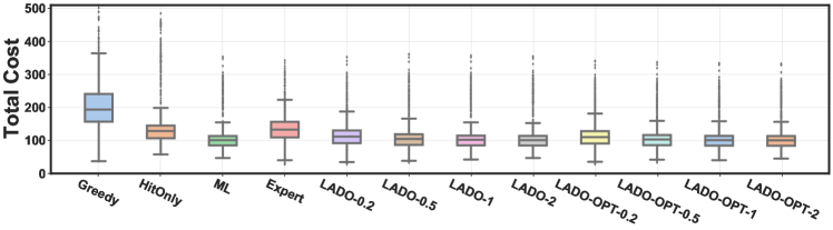
(a) Total cost

(b) Cost ratio of an algorithm to OPT

Figure 1: Comparison among different algorithms. The value $x$ in LADO-$x$ and LADO-OPT-$x$ refers to the parameter $\lambda=x$. The values in Fig. 1(b) is capped at 4.0 for better visualization.

B.2 Results

We first show the empirical average (AVG) and competitive ratio (CR) values in Table 1. The CR values are the empirically worst cost ratio of an algorithm’s cost to OPT’s cost in our testing dataset. We see from the table that Expert achieves the best empirical CR, but its average performance is not as good as ML due to its conservativeness. Although the pure ML-based optimizer achieves better average cost by leveraging historical data, its CR is significantly higher than Expert and even higher than Greedy.

By projecting the ML actions into carefully designed robust action sets, LADO can significantly reduce the CR compared to ML, while improving the average cost performance compared to Expert. Our analysis in Theorem 5.2 proves that, with a larger $\lambda$, the average cost of LADO is closer to that of ML. This point is also reflected by our experiments. Interestingly, by setting $\lambda=2$, LADO can even achieve a lower average cost than ML, while still having a lower CR. The reason is that Expert performs much better than ML for some problem instances. Thus, the inclusion of Expert in LADO avoids those instances that would otherwise have a high cost if ML were used, and meanwhile a large $\lambda=2$ also provides enough flexibility for LADO to exploit the benefits of ML in most other cases. Moreover, by training an ML policy that is explicitly aware of the projection, LADO-OPT can further reduce the average cost compared to LADO while having the same robustness guarantees.

Finally, we show the boxplots of total costs and cost ratios of different algorithms in Fig. 1. Here, the cost ratio is with respect to OPT. Note that the worst-case cost and cost ratio are different: a higher worst-case cost ratio of an algorithm ti OPT does not necessarily mean a higher worst-case cost. Our results complement Table 1 and show that LADO can achieve a lower cost than Expert in most problem instances while still having a significantly lower cost ratio than ML.

Appendix C Proof of Robustness in Theorem 5.1

We first prove the following lemma.

Lemma C.1.

If the spatial cost is non-negative, convex and $\ell_{S}$-smooth w,r,t the vector $(x_{v},x_{u})$, then for any $\lambda>0$, it holds that

$$s_{t}^{(v,u)}(x_{t}^{v},x_{t}^{u})-(1+\lambda)s_{t}^{(v,u)}(x_{t}^{v,\dagger},x_{t}^{u,\dagger})\leq\frac{\ell_{S}}{2}(1+\frac{1}{\lambda})\left(\|x_{t}^{v}-x_{t}^{v,\dagger}\|^{2}+\|x_{t}^{u}-x_{t}^{u,\dagger}\|^{2}\right).$$ (14)

Proof.

By the definition of smoothness, we have

$$s_{t}^{(v,u)}(x_{t}^{v},x_{t}^{u})$$ (15)

$$\leq s_{t}^{(v,u)}(x_{t}^{v,\dagger},x_{t}^{u,\dagger})+<\nabla s_{t}^{(v,u)}(x_{t}^{v,\dagger},x_{t}^{u,\dagger}),(x_{t}^{v}-x_{t}^{v,\dagger},x_{t}^{u}-x_{t}^{u,\dagger})>+\frac{\ell_{S}}{2}\|(x_{t}^{v},x_{t}^{u})-(x_{t}^{v,\dagger},x_{t}^{u,\dagger})\|^{2}$$

$$\leq s_{t}^{(v,u)}(x_{t}^{v,\dagger},x_{t}^{u,\dagger})+\|\nabla s_{t}^{(v,u)}(x_{t}^{v,\dagger},x_{t}^{u,\dagger})\|\cdot\|(x_{t}^{v}-x_{t}^{v,\dagger},x_{t}^{u}-x_{t}^{u,\dagger})\|+\frac{\ell_{S}}{2}\|(x_{t}^{v},x_{t}^{u})-(x_{t}^{v,\dagger},x_{t}^{u,\dagger})\|^{2}$$

$$\leq s_{t}^{(v,u)}(x_{t}^{v,\dagger},x_{t}^{u,\dagger})+\frac{\lambda}{2\ell_{S}}\|\nabla s_{t}^{(v,u)}(x_{t}^{v,\dagger},x_{t}^{u,\dagger})\|^{2}+(1+\frac{1}{\lambda})\frac{\ell_{S}}{2}\|(x_{t}^{v},x_{t}^{u})-(x_{t}^{v,\dagger},x_{t}^{u,\dagger})\|^{2}$$

The second inequality comes from the property of inner product. The third inequality is based on AM-QM inequality. Besides, if $(\hat{x}_{t}^{v},\hat{x}_{t}^{u})$ is a minimizer of the spatial cost, by Lemma 2.9 in [63], we have

$$s_{t}^{(v,u)}(x_{t}^{v,\dagger},x_{t}^{u,\dagger})\geq s_{t}^{(v,u)}(\hat{x}_{t}^{v},\hat{x}_{t}^{u})+0+\frac{1}{2\ell_{S}}\|\nabla s_{t}^{(v,u)}(x_{t}^{v,\dagger},x_{t}^{u,\dagger})\|^{2}\geq\frac{1}{2\ell_{S}}\|\nabla s_{t}^{(v,u)}(x_{t}^{v,\dagger},x_{t}^{u,\dagger})\|^{2}$$ (16)

By substituting Eqn (16) back to Eqn (15), we have

$$s_{t}^{(v,u)}(x_{t}^{v},x_{t}^{u})\leq(1+\lambda)\cdot s_{t}^{(v,u)}(x_{t}^{v,\dagger},x_{t}^{u,\dagger})+(1+\frac{1}{\lambda})\frac{\ell_{S}}{2}(\|(x_{t}^{v}-x_{t}^{v,\dagger}\|^{2}+\|x_{t}^{u}-x_{t}^{u,\dagger}\|^{2}).$$ (17)

∎

Proof of Theorem 5.1.

Proof.

To prove Theorem 5.1, the key point is to guarantee the robust action set (8) is non-empty. We will prove this through induction. For $t=1$, it is obvious that $x_{1}^{v}=x_{1}^{v,\dagger}$ satisfies the constraint. We assume that the robustness constraint is satisfied up to time step $t-1$, which is

$$\sum_{\tau=1}^{t-1}f_{\tau}^{v}(x_{\tau}^{v})+\sum_{\tau=1}^{t-2}\sum_{(v,u)\in\mathcal{E}}\kappa_{\tau}^{(v,u)}\cdot{s_{\tau}^{(v,u)}(x_{\tau}^{v},x_{\tau}^{u})}+\frac{\ell_{T}+\ell_{S}\cdot D_{v}}{2}(1+\frac{1}{\lambda_{0}})\cdot\|x_{t-1}^{v}-x_{t-1}^{v,\dagger}\|^{2}$$ (18)

$$+ \sum_{\tau=1}^{t-1}c_{\tau}^{v}(x_{\tau}^{v},x_{\tau-1}^{v})\leq(1+\lambda)\Bigl{(}\sum_{\tau=1}^{t-1}f_{\tau}^{v}(x_{\tau}^{v,\dagger})+\sum_{\tau=1}^{t-1}c_{\tau}^{v}(x_{\tau}^{v,\dagger},x_{\tau-1}^{v,\dagger})+\sum_{\tau=1}^{t-2}\sum_{(v,u)\in\mathcal{E}}\kappa_{\tau}^{(v,u)}\cdot{s_{\tau}^{(v,u)}(x_{\tau}^{v,\dagger},x_{\tau}^{u,\dagger})}\Bigr{)}$$

Based on Lemma C.1 and $\kappa_{t-1}^{(v,u)}=\frac{\|x_{t-1}^{v}-x_{t-1}^{v,\dagger}\|^{2}}{\|x_{t-1}^{v}-x_{t-1}^{v,\dagger}\|^{2}+\|x_{t-1}^{u}-x_{t-1}^{u,\dagger}\|^{2}}$, we have

$$\kappa_{t-1}^{(v,u)}\cdot\left({s_{t-1}^{(v,u)}(x_{t-1}^{v},x_{t-1}^{u})}-(1+\lambda)s_{t-1}^{(v,u)}(x_{t-1}^{v,\dagger},x_{t-1}^{u,\dagger})\right)\leq\frac{\ell_{S}}{2}(1+\frac{1}{\lambda})\|x_{t-1}^{v}-x_{t-1}^{v,\dagger}\|^{2}$$ (19)

For time step $t$, if we choose $x_{t}^{v}=x_{t}^{v,\dagger}$, by the smoothness assumption, we have

$$c_{t}^{v}(x_{t}^{v,\dagger},x_{t-1}^{v})-(1+\lambda)c_{t}^{v}(x_{t}^{v,\dagger},x_{t-1}^{v,\dagger}) \leq\frac{\ell_{T}}{2}(1+\frac{1}{\lambda})\|x_{t-1}^{v}-x_{t-1}^{v,\dagger}\|^{2}$$ (20)

Since the node cost is non-negative, by (19) and (20), we have

$$\begin{split}&f_{t}^{v}(x_{t}^{v,\dagger})+\sum_{(v,u)\in\mathcal{E}}\kappa_{t-1}^{(v,u)}\cdot{s_{t-1}^{(v,u)}(x_{t-1}^{v},x_{t-1}^{u})}+c_{t}^{v}(x_{t}^{v,\dagger},x_{t-1}^{v})-\frac{\ell_{T}+\ell_{S}\cdot D_{v}}{2}(1+\frac{1}{\lambda_{0}})\|x_{t-1}^{v}-x_{t-1}^{v,\dagger}\|^{2}\\ &-(1+\lambda)\Bigl{(}f_{t}^{v}(x_{t}^{v,\dagger})+c_{t}^{v}(x_{t}^{v,\dagger},x_{t-1}^{v,\dagger})+\sum_{(v,u)\in\mathcal{E}}\kappa_{t-1}^{(v,u)}\cdot{s_{t-1}^{(v,u)}(x_{t-1}^{v,\dagger},x_{t-1}^{u,\dagger})}\Bigr{)}\\ \leq&\frac{\ell_{T}+\ell_{S}\cdot D_{v}}{2}(1+\frac{1}{\lambda})\|x_{t-1}^{v}-x_{t-1}^{v,\dagger}\|^{2}-\frac{\ell_{T}+\ell_{S}\cdot D_{v}}{2}(1+\frac{1}{\lambda_{0}})\|x_{t-1}^{v}-x_{t-1}^{v,\dagger}\|^{2}\\ \leq&0,\end{split}$$ (21)

where the last inequality holds by $\lambda\geq\lambda_{0}$. By adding Eqn (21) back to Eqn (18) and moving items, we recover the robustness constraint for time step $t$ if $x_{t}^{v}=x_{t}^{v,\dagger}$,

$$\begin{gathered}\sum_{\tau=1}^{t}f_{\tau}^{v}(x_{\tau}^{v})+\sum_{\tau=1}^{t-1}\sum_{(v,u)\in\mathcal{E}}\kappa_{\tau}^{(v,u)}\cdot{s_{\tau}^{(v,u)}(x_{\tau}^{v},x_{\tau}^{u})}+\sum_{\tau=1}^{t}c_{\tau}^{v}(x_{\tau}^{v},x_{\tau-1}^{v})+\frac{\ell_{T}+\ell_{S}\cdot D_{v}}{2}(1+\frac{1}{\lambda_{0}})\|x_{t}^{v}-x_{t}^{v,\dagger}\|^{2}\\ \leq(1+\lambda)\Bigl{(}\sum_{\tau=1}^{t}f_{\tau}^{v}(x_{\tau}^{v,\dagger})+\sum_{\tau=1}^{t}c_{\tau}^{v}(x_{\tau}^{v,\dagger},x_{\tau-1}^{v,\dagger})+\sum_{\tau=1}^{t-1}\sum_{(v,u)\in\mathcal{E}}\kappa_{\tau}^{(v,u)}\cdot{s_{\tau}^{(v,u)}(x_{\tau}^{v,\dagger},x_{\tau}^{u,\dagger})}\Bigr{)}\end{gathered}$$ (22)

In other words, the expert’s action $x_{t}^{v,\dagger}$ is always an action in the corresponding robust action set (8). Thus the robust action set is non-empty.

Since $\kappa_{t}^{(v,u)}+\kappa_{t}^{(u,v)}=1$ holds for $(v,u)\in\mathcal{E}$, if all the nodes select actions from the robust action set (8) at each step, we can guarantee that $cost(\texttt{LADO},g_{1:T})\leq(1+\lambda)\cdot cost(\pi^{\dagger},g_{1:T})$ is satisfied. ∎

Appendix D Proof of Average Cost Bounds

D.1 Proof of Theorem 5.2

Lemma D.1.

We denote the actual actions from LADO as $x_{1:T}^{v}=(x_{1}^{v},\cdots,x_{T}^{v})$, the squared distance between actual action and ML advice is bounded by

$$\sum_{t=1}^{T}\|x_{t}^{v}-\tilde{x}_{t}^{v}\|^{2}\leq\sum_{t=1}^{T}\left[\|\tilde{x}^{v}_{t}-x_{t}^{v,\dagger}\|^{2}-{\frac{\lambda-\lambda_{0}}{1+\frac{1}{\lambda_{0}}}\cdot\frac{2}{\ell_{f}+2\cdot\ell_{T}+\ell_{S}\cdot D_{v}}\cdot\text{cost}_{v,t}^{\dagger}}\right]^{+}$$

where $\lambda$, $\lambda_{0}$, $D$, and $\rho$ are defined in Theorem 5.2.

Proof.

To prove this lemma, we first construct a sufficient condition to satisfy the original constraint in Eqn (5). Then we prove a distance bound in this sufficient condition, where the bound still holds for the original problem.

At time step $t$, we know the constraint in time step $t-1$ is already satisfied, so we obtain the following sufficient condition of the satisfaction of (5) as

$$\begin{gathered}f_{t}^{v}(x_{t}^{v})+\sum_{(v,u)\in\mathcal{E}}\kappa_{t-1}^{(v,u)}\cdot{s_{t-1}^{(v,u)}(x_{t-1}^{v},x_{t-1}^{u})}+\frac{\ell_{T}+\ell_{S}\cdot D_{v}}{2}(1+\frac{1}{\lambda_{0}})\left(\|x_{t}^{v}-x_{t}^{v,\dagger}\|^{2}-\|x_{t-1}^{v}-x_{t-1}^{v,\dagger}\|^{2}\right)\\ +c_{t}^{v}(x_{t}^{v},x_{t-1}^{v})\leq(1+\lambda)\Bigl{(}f_{t}^{v}(x_{t}^{v,\dagger})+c_{t}^{v}(x_{t}^{v,\dagger},x_{t-1}^{v,\dagger})+\sum_{(v,u)\in\mathcal{E}}\kappa_{t-1}^{(v,u)}\cdot{s_{t-1}^{(v,u)}(x_{t-1}^{v,\dagger},x_{t-1}^{u,\dagger})}\Bigr{)}\end{gathered}$$ (23)

With the convexity and smoothness assumptions, we have

$$c_{t}^{v}(x_{t}^{v,\dagger},x_{t-1}^{v})-(1+\lambda_{0})c_{t}^{v}(x_{t}^{v,\dagger},x_{t-1}^{v,\dagger}) \leq\frac{\ell_{T}}{2}(1+\frac{1}{\lambda_{0}})\left(\|x_{t}^{v}-x_{t}^{v,\dagger}\|^{2}+\|x_{t-1}^{v}-x_{t-1}^{v,\dagger}\|^{2}\right)$$ (24)

$$f_{t}^{v}(x_{t}^{v})-(1+\lambda_{0})f_{t}^{v}(x_{t}^{v,\dagger}) \leq\frac{\ell_{f}}{2}(1+\frac{1}{\lambda_{0}})\|x_{t}^{v}-x_{t}^{v,\dagger}\|^{2}$$

Then a sufficient condition that (23) holds becomes

$$\begin{gathered}\sum_{(v,u)\in\mathcal{E}}\kappa_{t-1}^{(v,u)}\cdot{s_{t-1}^{(v,u)}(x_{t-1}^{v},x_{t-1}^{u})}+(1+\frac{1}{\lambda_{0}})\left(\frac{\ell_{f}+2\cdot\ell_{T}+\ell_{S}\cdot D_{v}}{2}\|x_{t}^{v}-x_{t}^{v,\dagger}\|^{2}-\frac{\ell_{S}\cdot D_{v}}{2}\|x_{t-1}^{v}-x_{t-1}^{v,\dagger}\|^{2}\right)\\ \leq(\lambda-\lambda_{0})\Bigl{(}f_{t}^{v}(x_{t}^{v,\dagger})+c_{t}^{v}(x_{t}^{v,\dagger},x_{t-1}^{v,\dagger})\Bigr{)}+(1+\lambda)\sum_{(v,u)\in\mathcal{E}}\kappa_{t-1}^{(v,u)}\cdot{s_{t-1}^{(v,u)}(x_{t-1}^{v,\dagger},x_{t-1}^{u,\dagger})}\end{gathered}$$ (25)

From Eqn (19), we can further cancel out the spatial costs and get the sufficient condition as

$$\begin{gathered}(1+\frac{1}{\lambda_{0}})\left(\frac{\ell_{f}+2\cdot\ell_{T}+\ell_{S}\cdot D_{v}}{2}\|x_{t}^{v}-x_{t}^{v,\dagger}\|^{2}\right)\\ \leq(\lambda-\lambda_{0})\Bigl{(}f_{t}^{v}(x_{t}^{v,\dagger})+c_{t}^{v}(x_{t}^{v,\dagger},x_{t-1}^{v,\dagger})+\sum_{(v,u)\in\mathcal{E}}\kappa_{t-1}^{(v,u)}\cdot{s_{t-1}^{(v,u)}(x_{t-1}^{v,\dagger},x_{t-1}^{u,\dagger})}\Bigr{)}\end{gathered}$$ (26)

Therefore, for time step $t$, constraint (5) is satisfied if the action $x_{t}^{v}$ satisfies

$$\begin{gathered}{\|x_{t}^{v}-x_{t}^{v,\dagger}\|^{2}}\leq\frac{\lambda-\lambda_{0}}{1+\frac{1}{\lambda_{0}}}\cdot\frac{2}{\ell_{f}+2\cdot\ell_{T}+\ell_{S}\cdot D_{v}}\cdot\text{cost}_{v,t}^{\dagger}\end{gathered}$$ (27)

where $\text{cost}_{v,t}^{\dagger}$ denotes the cost of node $v$ at time $t$. Since actions that satisfy (27) must satisfy the original constraint (5) and $x_{t}^{v}$ is obtained by the projection from $\tilde{x}_{t}^{v}$ into the original constraint (5), we have

$$\|x_{t}^{v}-\tilde{x}_{t}^{v}\|\leq \left[{\|\tilde{x}^{v}_{t}-x_{t}^{v,\dagger}\|}-\sqrt{\frac{\lambda-\lambda_{0}}{1+\frac{1}{\lambda_{0}}}\cdot\frac{2}{\ell_{f}+2\cdot\ell_{T}+\ell_{S}\cdot D_{v}}\cdot\text{cost}_{v,t}^{\dagger}}\right]^{+}$$ (28)

Besides, it’s obvious that

$$\left(\left[{\|\tilde{x}^{v}_{t}-x_{t}^{v,\dagger}\|}-\sqrt{\frac{\lambda-\lambda_{0}}{1+\frac{1}{\lambda_{0}}}\cdot\frac{2}{\ell_{f}+2\cdot\ell_{T}+\ell_{S}\cdot D_{v}}\cdot\text{cost}_{v,t}^{\dagger}}\right]^{+}\right)^{2}$$ (29)

$$\leq \left[{\|\tilde{x}^{v}_{t}-x_{t}^{v,\dagger}\|}^{2}-{\frac{\lambda-\lambda_{0}}{1+\frac{1}{\lambda_{0}}}\cdot\frac{2}{\ell_{f}+2\cdot\ell_{T}+\ell_{S}\cdot D_{v}}\cdot\text{cost}_{v,t}^{\dagger}}\right]^{+}$$

By summing up the inequalities over time, we complete the proof. ∎

Proof of Theorem 5.2

Proof.

Based on the smoothness constraint, for any $\lambda_{2}>0$ we have

$$\left(\sum_{\tau=1}^{T}f_{\tau}^{v}(x_{\tau}^{v})+\sum_{\tau=1}^{T}c_{\tau}^{v}(x_{\tau}^{v},x_{\tau-1}^{v})\right)-(1+\lambda_{2})\left(\sum_{\tau=1}^{T}f_{\tau}^{v}(\tilde{x}_{\tau}^{v})+\sum_{\tau=1}^{T}c_{\tau}^{v}(\tilde{x}_{\tau}^{v},\tilde{x}_{\tau-1}^{v})\right)$$ (30)

$$\leq (1+\frac{1}{\lambda_{2}})\left(\frac{\ell_{f}}{2}\sum_{\tau=1}^{T}\|x_{\tau}^{v}-\tilde{x}_{\tau}^{v}\|^{2}+\frac{\ell_{T}}{2}\sum_{\tau=1}^{T}\|x_{\tau}^{v}-\tilde{x}_{\tau}^{v}\|^{2}+\frac{\ell_{T}}{2}\sum_{\tau=0}^{T-1}\|x_{\tau}^{v}-\tilde{x}_{\tau}^{v}\|^{2}\right)$$

$$\leq (1+\frac{1}{\lambda_{2}})\frac{\ell_{f}+2\cdot\ell_{T}}{2}\sum_{\tau=1}^{T}\|x_{\tau}^{v}-\tilde{x}_{\tau}^{v}\|^{2}$$

Similarly, according to Eqn (19), by summing up the inequalities over time, we have

$$\sum_{(v,u)\in\mathcal{E}}\sum_{\tau=1}^{T}\kappa_{\tau}^{(v,u)}\cdot{s_{\tau}^{(v,u)}(x_{\tau}^{v},x_{\tau}^{u})}-(1+\lambda_{2})\sum_{(v,u)\in\mathcal{E}}\sum_{\tau=1}^{T}\kappa_{\tau}^{(v,u)}\cdot{s_{\tau}^{(v,u)}(\tilde{x}_{\tau}^{v},\tilde{x}_{\tau}^{u})}$$ (31)

$$\leq (1+\frac{1}{\lambda_{2}})\frac{\ell_{S}}{2}\sum_{(v,u)\in\mathcal{E}}\sum_{\tau=1}^{T}\|x_{\tau}^{v}-\tilde{x}_{\tau}^{v}\|^{2}=(1+\frac{1}{\lambda_{2}})\frac{D_{v}\cdot\ell_{S}}{2}\sum_{\tau=1}^{T}\|x_{\tau}^{v}-\tilde{x}_{\tau}^{v}\|^{2}$$

By adding Eqn (30) and Eqn (31), we can bound the cost error of node $v$ as

$$\text{cost}_{v}({x}_{1:T}^{v})-(1+\lambda_{2})\text{cost}_{v}(\tilde{x}_{1:T}^{v}) \leq(1+\frac{1}{\lambda_{2}})\frac{\ell_{f}+2\cdot\ell_{T}+D_{v}\cdot\ell_{S}}{2}\sum_{\tau=1}^{T}\|x_{\tau}^{v}-\tilde{x}_{\tau}^{v}\|^{2}$$ (32)

By substituting Lemma D.1 into Eqn (32), we have

$$\text{cost}_{v}({x}_{1:T}^{v})-(1+\lambda_{2})\text{cost}_{v}(\tilde{x}_{1:T}^{v})\leq(1+\frac{1}{\lambda_{2}})\frac{\ell_{f}+2\cdot\ell_{T}+\ell_{S}\cdot D_{v}}{2}\omega_{v}(\lambda)$$ (33)

we denote $\omega_{v}(\lambda)=\sum_{t=1}^{T}\left[\|\tilde{x}^{v}_{t}-x_{t}^{v,\dagger}\|^{2}-\frac{2}{\ell_{f}+2\cdot\ell_{T}+\ell_{S}\cdot D_{v}}\cdot{\frac{\lambda-\lambda_{0}}{1+\frac{1}{\lambda_{0}}}\cdot\text{cost}_{v,t}^{\dagger}}\right]^{+}$ as the auxiliary cost brought by the robustification process. By summing up the cost all nodes $v\in\mathcal{V}$ and taking the expectation over $g_{1:T}\in\mathcal{G}$ over the data distribution, the average cost of our algorithm is bounded by

$${AVG}(\texttt{LADO}(\tilde{\pi}))-(1+\lambda_{2}){AVG}(\tilde{\pi})\leq(1+\frac{1}{\lambda_{2}})\frac{\ell_{f}+2\cdot\ell_{T}+\ell_{S}\cdot D_{v}}{2}\cdot\Omega(\lambda,\tilde{\pi},\pi^{\dagger})$$ (34)

where $\Omega(\lambda,\tilde{\pi},\pi^{\dagger})=\mathbb{E}_{g_{1:T}}[\sum_{v\in\mathcal{V}}\omega_{v}(\lambda)]$. By optimally setting $\lambda_{2}=\sqrt{\frac{\ell_{f}+2\ell_{T}+\ell_{S}D_{v}}{2}\cdot\frac{\Omega(\lambda,\tilde{\pi},\pi^{\dagger})}{{AVG}(\tilde{\pi})}}$, we finish the proof for the second term in the min operator

$${AVG}(\texttt{LADO}(\tilde{\pi}))\leq\biggl{(}\sqrt{{AVG}(\tilde{\pi})}+\sqrt{\frac{\ell_{f}+2\ell_{T}+\ell_{S}D_{v}}{2}\cdot\Omega(\lambda,\tilde{\pi},\pi^{\dagger})}\biggr{)}^{2}$$ (35)

The first term in the min operator can be directly obtained by Theorem 5.1. ∎

D.2 Proof of Corollary 5.3

Proof.

In Corollary 5.3, we assume that $\pi_{\lambda}^{\circ}$ in Eqn. (10) is used in LADO. To bound the average cost of $\texttt{LADO}(\tilde{\pi}_{\lambda}^{\circ})$, we construct a policy that satisfies the constraint (5) for each step in each sequence. Then the average cost bound of the constructed policy is also the average cost upper bound of $\texttt{LADO}(\tilde{\pi}_{\lambda}^{\circ})$ since $\texttt{LADO}(\tilde{\pi}_{\lambda}^{\circ})$ is the policy that minimizes average cost while satisfying the constraint (5) for each step in each sequence if we assume that the ML model can represent any policy. The feasible policy is constructed as $\hat{\pi}=(1-\alpha)\pi^{\dagger}+\alpha\tilde{\pi}^{*}$ which gives action $\hat{x}_{t}^{v}=(1-\alpha)x_{t}^{v,\dagger}+\alpha\tilde{x}_{t}^{v},\alpha\in[0,1]$, where $x_{t}^{\dagger}$, $\tilde{x}_{t}$ denotes expert action and the prediction from projection-unaware ML model $\tilde{\pi}^{*}$, respectively. We need to find the $\alpha$ that guarantees the satisfaction of the constraint (3). To do that, we rewrite the constraint as

$$\sum_{\tau=1}^{t}\Bigl{(}f_{\tau}^{v}(\hat{x}_{\tau}^{v})-(1+\lambda_{0})f_{\tau}^{v}(x_{\tau}^{\dagger})\Bigr{)}+\sum_{\tau=1}^{t}\left(c^{v}(\hat{x}_{\tau}^{v},\hat{x}_{\tau-1}^{v})-(1+\lambda_{0})c^{v}(x_{\tau}^{v,\dagger},x_{\tau-1}^{v,\dagger})\right)+\sum_{\tau=1}^{t-1}\sum_{(v,u)\in\mathcal{E}}\kappa_{\tau}^{(v,u)}\cdot$$ (36)

$$\Bigl{(}{s_{\tau}^{(v,u)}(\hat{x}_{\tau}^{v},\hat{x}_{\tau}^{u})}-(1+\lambda_{0}){s_{\tau}^{(v,u)}(x_{\tau}^{v,\dagger},x_{\tau}^{u,\dagger})}\Bigr{)}+(1+\frac{1}{\lambda_{0}})\frac{\ell_{T}+D_{v}\cdot\ell_{S}}{2}\|x_{t}^{v}-x_{t}^{v,\dagger}\|^{2}$$

$$\leq (\lambda-\lambda_{0})\Bigl{(}\sum_{\tau=1}^{t}f_{\tau}^{v}({x}_{\tau}^{v,\dagger})+\sum_{\tau=1}^{t}c^{v}(x_{\tau}^{v,\dagger},x_{\tau-1}^{v,\dagger})+\sum_{\tau=1}^{t-1}\sum_{(v,u)\in\mathcal{E}}\kappa_{\tau}^{(v,u)}s_{\tau}^{(v,u)}(x_{\tau}^{v,\dagger},x_{\tau}^{u,\dagger})\Bigr{)},\forall t\in[1,T]$$

Based on the smoothness assumption, we have

$$f_{t}^{v}(\hat{x}_{t}^{v})-(1+\lambda_{0})f_{t}^{v}(x_{t}^{v,\dagger})\leq (1+\frac{1}{\lambda_{0}})\frac{\ell_{f}}{2}\|\hat{x}_{t}^{v}-x_{t}^{v,\dagger}\|^{2}$$ (37)

$$c^{v}(\hat{x}_{t}^{v},\hat{x}_{t-1}^{v})-(1+\lambda_{0})c^{v}(x_{t}^{v,\dagger},x_{t-1}^{v,\dagger})\leq (1+\frac{1}{\lambda_{0}})\frac{\ell_{T}}{2}(\|\hat{x}_{t}^{v}-x_{t}^{v,\dagger}\|^{2}+\|\hat{x}_{t-1}^{v}-x_{t-1}^{v,\dagger}\|^{2})$$

$$\kappa_{t}^{(v,u)}\left({s_{t}^{(v,u)}(\hat{x}_{t}^{v},\hat{x}_{t}^{u})}-(1+\lambda_{0}){s_{t}^{(v,u)}(x_{t}^{v,\dagger},x_{t}^{u,\dagger})}\right)\leq (1+\frac{1}{\lambda_{0}})\frac{\ell_{S}}{2}(\|\hat{x}_{t}^{v}-x_{t}^{v,\dagger}\|^{2})$$

Then, a sufficient condition of Eqn (36) is

$$\begin{gathered}(1+\frac{1}{\lambda_{0}})\frac{\ell_{f}+2\ell_{T}+D_{v}\ell_{S}}{2}\sum_{\tau=1}^{t}\|\hat{x}_{\tau}^{v}-x_{\tau}^{v,\dagger}\|^{2}\leq(\lambda-\lambda_{0})\text{cost}_{v}(x_{1:t}^{v,\dagger}),\forall t\in[1,T]\end{gathered}$$ (38)

Since $D=\max_{v\in\mathcal{V}}D_{v}$ is the maximum node degree in the whole graph, then

$$\alpha^{2}\sum_{\tau=1}^{t}\|\tilde{x}_{\tau}^{v}-x_{\tau}^{v,\dagger}\|^{2}\leq\frac{2}{\ell_{f}+2\ell_{T}+D\cdot\ell_{S}}\cdot\frac{\lambda-\lambda_{0}}{1+\frac{1}{\lambda_{0}}}\text{cost}_{v}(x_{1:t}^{v,\dagger}),\forall t\in[1,T]$$ (39)

We define $\hat{C}=\min_{v\in\mathcal{V},t\in[1,T]}\frac{\text{cost}_{v}(x_{1:t}^{v,\dagger})}{\sum_{i=1}^{t}\|x_{i}^{v,\dagger}-\tilde{x}_{i}^{v}\|^{2}}$ as the minimum normalized baseline cost, then we can have

$$\alpha\leq\min\left\{1,\sqrt{\frac{2}{\ell_{f}+2\ell_{T}+D\cdot\ell_{S}}\cdot\frac{\lambda-\lambda_{0}}{1+\frac{1}{\lambda_{0}}}\cdot\hat{C}}\right\}=\alpha_{\lambda}$$ (40)

In other words, as long as $\alpha\in[0,\alpha_{\lambda}]$, the robustness constraint is always satisfied. Based on the convex assumption on hitting cost, temporal cost and spatial cost, we have

$$\text{cost}_{v}(\hat{x}_{1:t}^{v})=\text{cost}_{v}((1-\alpha){x}_{1:t}^{v,\dagger}+\alpha\tilde{x}_{1:t}^{v,\dagger})\leq(1-\alpha)\text{cost}_{v}({x}_{1:t}^{v,\dagger})+\alpha\cdot\text{cost}_{v}(\tilde{x}_{1:t}^{v}).$$ (41)

By setting $\alpha=\alpha_{\lambda}$ and taking expectation of both side over the data distribution, we finish the proof of the first term in Theorem 5.3. ∎

References

- [1] Hamidreza Shahbazi and Farid Karbalaei. Decentralized voltage control of power systems using multi-agent systems. Journal of Modern Power Systems and Clean Energy, 8(2):249–259, 2020.
- [2] Yuanyuan Shi, Guannan Qu, Steven Low, Anima Anandkumar, and Adam Wierman. Stability constrained reinforcement learning for real-time voltage control. arXiv preprint arXiv:2109.14854, 2021.
- [3] Saghar Hosseini, Airlie Chapman, and Mehran Mesbahi. Online distributed convex optimization on dynamic networks. IEEE Transactions on Automatic Control, 61(11):3545–3550, 2016.
- [4] Songchun Fan, Seyed Majid Zahedi, and Benjamin C. Lee. The computational sprinting game. In ASPLOS, 2016.
- [5] Amal Feriani and Ekram Hossain. Single and multi-agent deep reinforcement learning for ai-enabled wireless networks: A tutorial. IEEE Communications Surveys & Tutorials, 23(2):1226–1252, 2021.
- [6] Yasar Sinan Nasir and Dongning Guo. Multi-agent deep reinforcement learning for dynamic power allocation in wireless networks. IEEE Journal on Selected Areas in Communications, 37(10):2239–2250, 2019.
- [7] Fuqiang Yao and Luliang Jia. A collaborative multi-agent reinforcement learning anti-jamming algorithm in wireless networks. IEEE wireless communications letters, 8(4):1024–1027, 2019.
- [8] Felipe Caro and Jérémie Gallien. Clearance pricing optimization for a fast-fashion retailer. Operations research, 60(6):1404–1422, 2012.
- [9] Ozan Candogan, Kostas Bimpikis, and Asuman Ozdaglar. Optimal pricing in networks with externalities. Operations Research, 60(4):883–905, 2012.
- [10] Alec Koppel, Felicia Y. Jakubiec, and Alejandro Ribeiro. A saddle point algorithm for networked online convex optimization. IEEE Transactions on Signal Processing, 63(19):5149–5164, 2015.
- [11] Xuanyu Cao and Tamer Başar. Decentralized online convex optimization based on signs of relative states. Automatica, 129:109676, 2021.
- [12] Kaixiang Lin, Shu Wang, and Jiayu Zhou. Collaborative deep reinforcement learning. arXiv preprint arXiv:1702.05796, 2017.
- [13] Xuanyu Cao and Tamer Başar. Decentralized online convex optimization with feedback delays. IEEE Transactions on Automatic Control, 67(6):2889–2904, 2021.
- [14] Mehrdad Mahdavi, Rong Jin, and Tianbao Yang. Trading regret for efficiency: Online convex optimization with long term constraints. J. Mach. Learn. Res., 13(1):2503–2528, sep 2012.
- [15] Gautam Goel and Adam Wierman. An online algorithm for smoothed online convex optimization. SIGMETRICS Perform. Eval. Rev., 47(2):6–8, December 2019.
- [16] Gautam Goel, Yiheng Lin, Haoyuan Sun, and Adam Wierman. Beyond online balanced descent: An optimal algorithm for smoothed online optimization. In NeurIPS, volume 32, 2019.
- [17] Lijun Zhang, Wei Jiang, Shiyin Lu, and Tianbao Yang. Revisiting smoothed online learning. In A. Beygelzimer, Y. Dauphin, P. Liang, and J. Wortman Vaughan, editors, Advances in Neural Information Processing Systems, 2021.
- [18] Guanya Shi, Yiheng Lin, Soon-Jo Chung, Yisong Yue, and Adam Wierman. Online optimization with memory and competitive control. Advances in Neural Information Processing Systems, 33:20636–20647, 2020.
- [19] Weici Pan, Guanya Shi, Yiheng Lin, and Adam Wierman. Online optimization with feedback delay and nonlinear switching cost. Proc. ACM Meas. Anal. Comput. Syst., 6(1), feb 2022.
- [20] Niangjun Chen, Gautam Goel, and Adam Wierman. Smoothed online convex optimization in high dimensions via online balanced descent. In COLT, 2018.
- [21] Xiuxian Li, Xinlei Yi, and Lihua Xie. Distributed online convex optimization with an aggregative variable. IEEE Transactions on Control of Network Systems, 2021.
- [22] Saghar Hosseini, Airlie Chapman, and Mehran Mesbahi. Online distributed convex optimization on dynamic networks. IEEE Transactions on Automatic Control, 61(11):3545–3550, 2016.
- [23] Weiwei Kong, Christopher Liaw, Aranyak Mehta, and D. Sivakumar. A new dog learns old tricks: RL finds classic optimization algorithms. In ICLR, 2019.
- [24] Thomas Barrett, William Clements, Jakob Foerster, and Alex Lvovsky. Exploratory combinatorial optimization with reinforcement learning. In AAAI, 2020.
- [25] Han Zhang, Wenzhong Li, Shaohua Gao, Xiaoliang Wang, and Baoliu Ye. Reles: A neural adaptive multipath scheduler based on deep reinforcement learning. In INFOCOM, 2019.
- [26] Zhihui Shao, Jianyi Yang, Cong Shen, and Shaolei Ren. Learning for robust combinatorial optimization: Algorithm and application. In INFOCOM, 2022.
- [27] Kaiqing Zhang, Zhuoran Yang, Han Liu, Tong Zhang, and Tamer Basar. Fully decentralized multi-agent reinforcement learning with networked agents. In International Conference on Machine Learning, pages 5872–5881. PMLR, 2018.
- [28] Kaiqing Zhang, Zhuoran Yang, and Tamer Başar. Multi-agent reinforcement learning: A selective overview of theories and algorithms. Handbook of Reinforcement Learning and Control, pages 321–384, 2021.
- [29] Afshin Oroojlooy and Davood Hajinezhad. A review of cooperative multi-agent deep reinforcement learning. Applied Intelligence, pages 1–46, 2022.
- [30] Pengfei Li, Jianyi Yang, and Shaolei Ren. Robustified learning for online optimization with memory costs. In INFOCOM, 2023.
- [31] Nicolas Christianson, Tinashe Handina, and Adam Wierman. Chasing convex bodies and functions with black-box advice. In COLT, 2022.
- [32] Joan Boyar, Lene M. Favrholdt, Christian Kudahl, Kim S. Larsen, and Jesper W. Mikkelsen. Online algorithms with advice: A survey. SIGACT News, 47(3):93–129, August 2016.
- [33] Alexander Wei and Fred Zhang. Optimal robustness-consistency trade-offs for learning-augmented online algorithms. In NeurIPS, 2020.
- [34] Étienne Bamas, Andreas Maggiori, and Ola Svensson. The primal-dual method for learning augmented algorithms. Advances in Neural Information Processing Systems, 33:20083–20094, 2020.
- [35] Thodoris Lykouris and Sergei Vassilvitskii. Competitive caching with machine learned advice. J. ACM, 68(4), July 2021.
- [36] Zhipeng Tu, Xi Wang, Yiguang Hong, Lei Wang, Deming Yuan, and Guodong Shi. Distributed online convex optimization with compressed communication. In S. Koyejo, S. Mohamed, A. Agarwal, D. Belgrave, K. Cho, and A. Oh, editors, Advances in Neural Information Processing Systems, volume 35, pages 34492–34504. Curran Associates, Inc., 2022.
- [37] Yiheng Lin, Judy Gan, Guannan Qu, Yash Kanoria, and Adam Wierman. Decentralized online convex optimization in networked systems. In Kamalika Chaudhuri, Stefanie Jegelka, Le Song, Csaba Szepesvari, Gang Niu, and Sivan Sabato, editors, Proceedings of the 39th International Conference on Machine Learning, volume 162 of Proceedings of Machine Learning Research, pages 13356–13393. PMLR, 17–23 Jul 2022.
- [38] Yifan Wu, Roshan Shariff, Tor Lattimore, and Csaba Szepesvári. Conservative bandits. In International Conference on Machine Learning, pages 1254–1262. PMLR, 2016.
- [39] Yunchang Yang, Tianhao Wu, Han Zhong, Evrard Garcelon, Matteo Pirotta, Alessandro Lazaric, Liwei Wang, and Simon Shaolei Du. A reduction-based framework for conservative bandits and reinforcement learning. In International Conference on Learning Representations, 2021.
- [40] Evrard Garcelon, Mohammad Ghavamzadeh, Alessandro Lazaric, and Matteo Pirotta. Conservative exploration in reinforcement learning. In Silvia Chiappa and Roberto Calandra, editors, Proceedings of the Twenty Third International Conference on Artificial Intelligence and Statistics, volume 108 of Proceedings of Machine Learning Research, pages 1431–1441. PMLR, 26–28 Aug 2020.
- [41] M. Lin, A. Wierman, L. L. H. Andrew, and E. Thereska. Dynamic right-sizing for power-proportional data centers. In INFOCOM, 2011.
- [42] Mohammad A. Islam, Kishwar Ahmed, Hong Xu, Nguyen H. Tran, Gang Quan, and Shaolei Ren. Exploiting spatio-temporal diversity for water saving in geo-distributed data centers. IEEE Transactions on Cloud Computing, 6(3):734–746, 2018.
- [43] Meta. Sustainability report, 2021, https://sustainability.fb.com/.
- [44] Gautam Goel, Yiheng Lin, Haoyuan Sun, and Adam Wierman. Beyond online balanced descent: An optimal algorithm for smoothed online optimization. Advances in Neural Information Processing Systems, 32, 2019.
- [45] Richard Cheng, Abhinav Verma, Gabor Orosz, Swarat Chaudhuri, Yisong Yue, and Joel Burdick. Control regularization for reduced variance reinforcement learning. In Kamalika Chaudhuri and Ruslan Salakhutdinov, editors, Proceedings of the 36th International Conference on Machine Learning, volume 97 of Proceedings of Machine Learning Research, pages 1141–1150. PMLR, 09–15 Jun 2019.
- [46] Hoang M. Le, Andrew Kang, Yisong Yue, and Peter Carr. Smooth imitation learning for online sequence prediction. In ICML, 2016.
- [47] Yunchang Yang, Tianhao Wu, Han Zhong, Evrard Garcelon, Matteo Pirotta, Alessandro Lazaric, Liwei Wang, and Simon Shaolei Du. A reduction-based framework for conservative bandits and reinforcement learning. In International Conference on Learning Representations, 2022.
- [48] Jakub Chłędowski, Adam Polak, Bartosz Szabucki, and Konrad Tomasz Żołna. Robust learning-augmented caching: An experimental study. In ICML, 2021.
- [49] Keerti Anand, Rong Ge, Amit Kumar, and Debmalya Panigrahi. A regression approach to learning-augmented online algorithms. In A. Beygelzimer, Y. Dauphin, P. Liang, and J. Wortman Vaughan, editors, Advances in Neural Information Processing Systems, 2021.
- [50] Manish Purohit, Zoya Svitkina, and Ravi Kumar. Improving online algorithms via ml predictions. In NeurIPS, 2018.
- [51] Goran Zuzic, Di Wang, Aranyak Mehta, and D. Sivakumar. Learning robust algorithms for online allocation problems using adversarial training. In https://arxiv.org/abs/2010.08418, 2020.
- [52] Daan Rutten, Nicolas Christianson, Debankur Mukherjee, and Adam Wierman. Smoothed online optimization with unreliable predictions. Proc. ACM Meas. Anal. Comput. Syst., 7(1), mar 2023.
- [53] Antonios Antoniadis, Christian Coester, Marek Elias, Adam Polak, and Bertrand Simon. Online metric algorithms with untrusted predictions. In ICML, 2020.
- [54] Yiheng Lin, Yang Hu, Guannan Qu, Tongxin Li, and Adam Wierman. Bounded-regret MPC via perturbation analysis: Prediction error, constraints, and nonlinearity. In Alice H. Oh, Alekh Agarwal, Danielle Belgrave, and Kyunghyun Cho, editors, Advances in Neural Information Processing Systems, 2022.
- [55] Akshay Agrawal, Brandon Amos, Shane Barratt, Stephen Boyd, Steven Diamond, and J. Zico Kolter. Differentiable convex optimization layers. In H. Wallach, H. Larochelle, A. Beygelzimer, F. d'Alché-Buc, E. Fox, and R. Garnett, editors, Advances in Neural Information Processing Systems, volume 32. Curran Associates, Inc., 2019.
- [56] Ana Radovanović, Ross Koningstein, Ian Schneider, Bokan Chen, Alexandre Duarte, Binz Roy, Diyue Xiao, Maya Haridasan, Patrick Hung, Nick Care, Saurav Talukdar, Eric Mullen, Kendal Smith, MariEllen Cottman, and Walfredo Cirne. Carbon-aware computing for datacenters. IEEE Transactions on Power Systems, 38(2):1270–1280, 2023.
- [57] U.S. Department of Engergy. What is environmental justice?, https://www.energy.gov/lm/what-environmental-justice.
- [58] Le Yi Wang, Caisheng Wang, George Yin, Feng Lin, Michael P. Polis, Caiping Zhang, and Jiuchun Jiang. Balanced control strategies for interconnected heterogeneous battery systems. IEEE Transactions on Sustainable Energy, 7(1):189–199, 2016.
- [59] Eli Cortez, Anand Bonde, Alexandre Muzio, Mark Russinovich, Marcus Fontoura, and Ricardo Bianchini. Resource central: Understanding and predicting workloads for improved resource management in large cloud platforms. In Proceedings of the 26th Symposium on Operating Systems Principles, pages 153–167, 2017.
- [60] Manajit Sengupta, Yu Xie, Anthony Lopez, Aron Habte, Galen Maclaurin, and James Shelby. The national solar radiation data base (nsrdb). Renewable and sustainable energy reviews, 89:51–60, 2018.
- [61] Can Wan, Jian Zhao, Yonghua Song, Zhao Xu, Jin Lin, and Zechun Hu. Photovoltaic and solar power forecasting for smart grid energy management. CSEE Journal of Power and Energy Systems, 1(4):38–46, 2015.
- [62] Asis Sarkar and Dhiren Kumar Behera. Wind turbine blade efficiency and power calculation with electrical analogy. International Journal of Scientific and Research Publications, 2(2):1–5, 2012.
- [63] Moritz Hardt and Max Simchowitz. Convex optimization and approximation. https://ee227c.github.io/notes/ee227c-notes.pdf, 2018.